Analysis of Contact-Voltage Losses in Low-Voltage Electricity Distribution Systems of the U.K.

Dr. Eric D. Larson

PI, Energy Systems Analysis Group Andlinger Center for Energy & Environment

Princeton University, Princeton, NJ, USA

Prof. Minjie Chen PI, Princeton Power Electronics Research Lab

Department of Electrical Engineering Andlinger Center for Energy & Environment

Princeton University, Princeton, NJ, USA

FINAL REPORT

Prepared under contract for UK Power Networks (UKPN) Project manager:

Mr. Jeremy L. Wright, BEng (Hons) MBA CEng FIET FCMI MIAM Asset Inspection, Maintenance, and Compliance Manager

Asset Management UKPN

January 30, 2018

2

Analysis of Contact-Voltage Losses in Low-Voltage Electricity Distribution Systems of the U.K.

Table of Contents List of Tables .................................................................................................................................. 3 List of Figures ................................................................................................................................. 3

Executive Summary ........................................................................................................................ 4

1 Contact-voltage faults .............................................................................................................. 5

2 Technical, non-technical, and contact-voltage losses from the UK grid ................................. 5 3 Methods for detecting contact voltages ................................................................................... 6

4 MAAV-detected contact-voltage loss estimates for Central London ...................................... 7

5 Estimated contact-voltage losses across the UK ..................................................................... 9

6 Contact-voltage loss estimate in perspective ......................................................................... 13 7 Cost-benefit analysis of MAAV-based CV detection and repair .......................................... 13

7.1 The business-as-usual (BAU) scenario .............................................................................. 13

7.2 Additional assumptions for the cost-benefit analysis ........................................................ 15

7.3 Results ................................................................................................................................ 17 8 Conclusions and some reflections ......................................................................................... 18

9 References ............................................................................................................................. 19

3

List of Tables Table 1. UK electricity supply, losses, and final consumption (TWh/year). ......................................... 5

Table 2. Summary results of UKPN’s Central London MAAV survey and corresponding estimated electricity losses. .................................................................................................................................... 7

Table 3. Parameter values and resulting impedance to ground and electricity losses for each phase-side cable contact voltage identified in Central London. ....................................................................... 9

Table 4. Parameter values and resulting impedances to ground from Equation 2 for 18 different lighting column designs used by the city of London ().a ....................................................................... 9

Table 5. Results of MAAV surveys for contact voltages in distribution networks in municipalities served by Consolidated Edison of New York. ..................................................................................... 10

Table 6. Central London MAAV survey results. ................................................................................. 11

Table 7. DNO-specific loss estimates for phase-side cable and phase-side lighting column contact voltages. ............................................................................................................................................... 12

Table 8. Estimated lengths of underground low-voltage cable miles in each DNO and the corresponding estimated contact-voltage MWh losses that could be avoided annually ...................... 12

Table 9. Estimated loss reduction potential across UK DNOs via implementation of various measures [3]. ........................................................................................................................................................ 13

Table 10. Number of objects energized (to one volt or higher) by contact voltages identified via MAAV surveys each year by Consolidated Edison of New York, Inc. across its full service territory............................................................................................................................................................... 14

Table 11. Input assumptions for cost-benefit analysis. ........................................................................ 16

Table 12. Valuations of costs and benefits associated with MAAV detection and repair of contact voltages.a .............................................................................................................................................. 16

Table 13. Greenhouse gas (GHG) emission trading prices, air pollution damage costs, and grid electricity GHG emissions recommended by the UK government (BEIS) and by OFGEM for use in appraisals. The analysis in this report uses the OFGEM values where available. .............................. 17

List of Figures Figure 1. Soil resistivity map of Great Britain (left) and DNO operating territories (right). ............... 11

Figure 2. Illustration of the number of unrepaired CVs that would exist in the BAU scenario for each CV that would have been detected and repaired had a MAAV program been implemented. This illustration assumes that each CV in the BAU scenario persists for three years before it is repaired. 15

Figure 3. Discounted annual costs and benefits (left axis) and cumulative discounted net benefits (right axis) for an 8-year MAAV-based CV detection and repair program, assuming CVs persist for 1 year in the BAU scenario. .................................................................................................................... 17

Figure 4. Discounted annual costs and benefits for an 8-year MAAV-based CV detection and repair program with different assuming CV lifetimes in the BAU scenario. ................................................. 18

4

Executive Summary Underground contact voltages (CV) commonly result from a break in the insulation of a

conductor due to accidental damage during construction work, chemical corrosion, degradation with aging, or other factors. Electricity losses due to such CVs on distribution networks in the UK are estimated in this report to be about 0.59 TWh per year. The unmetered portion of these account for 2.5% of what are traditionally categorized as technical losses from UK distribution networks. CV loss appears to be the single largest avoidable electricity loss on UK networks.

CVs can be detected quickly and efficiently using non-contact mobile methods, as has been demonstrated annually in New York City for more than a decade and in a Central London trial that began in late 2016. In London, a Mobile Asset Assessment Vehicle (MAAV) traversed 425 roadway miles and identified 62 occurrences of CV. Estimating the associated losses using well-established methodologies and extrapolating the loss estimates to the full London Power Network (LPN) license area indicates that some 38 GWh per year of electricity are being lost in the LPN area through CVs. Further extrapolating these findings to distribution networks across the UK gives 0.59 TWh per year of UK-wide losses.

The cost for MAAV-based detection and remediation of CV losses in the UK would be more than offset by the associated benefits, based on the analysis in this report. A key uncertainty is the length of time that a CV would persist in the absence of a MAAV program before it would be detected and repaired. The longer lived a CV would have been, the larger is the benefit of implementing a MAAV program. The cost-benefit ratio is clearly positive even with an assumed CV lifetime of just one year.

5

1 Contact-voltage faults The IEEE’s Guide to Understanding, Diagnosing, and Mitigating Stray and Contact

Voltage1 defines contact voltage as “a voltage resulting from electrical faults that may be present between two conductive surfaces that can be simultaneously contacted by members of the general public or animals. Contact voltage can exist at levels that may be hazardous.” CV faults can occur on both overhead lines and underground cables. On overhead lines they are typically readily visible (e.g., electric arcs) and easily and quickly repaired. On the other hand, detecting CV faults on underground cables is more challenging, and repairing them is more involved than repairing faults on overhead lines. Underground cables are found in most populated urban areas of the UK. Contact-voltage faults on underground cables are the focus of this report.

Underground CV commonly results from a break in the insulation of a conductor as a result of accidental damage during construction work, chemical corrosion, degradation with aging, or other external factors. The break allows electricity to leak to ground and/or to energize conducting objects such as manhole covers or lighting columns. Such breaks have minor or even undetectable impacts on a grid’s operation. However, they raise public safety concerns and leak energy into the surrounding environment until repaired. The continuous leakage of energy over time can represent substantial cumulative losses.

2 Technical, non-technical, and contact-voltage losses from the UK grid Losses of all types in electricity networks in the UK totaled about 26 TWh during 2016

(Table 1). This is 7.7% of total electricity supplied from power plants, or equivalent to the annual output of four large (1000 MW) baseload generating units. Losses in the high-voltage transmission system are not insignificant, but these are relatively well understood, closely monitored, and mitigated to the extent practicable. On the other hand, losses in low-voltage distribution systems account for approximately 75% of all losses (assuming “Theft” in Table 1 is associated primarily with the distribution system).

Table 1. UK electricity supply, losses, and final consumption (TWh/year).2 2014 2015 2016

Electricity supplied 342 343 342 Total losses 28.5 27.3 26.3

Transmission 6.51 7.40 7.40 Distribution 21.14 19.07 18.91

Theft 1.00 1.00 1.00 Final consumption 303 303 304

Conventionally, electricity losses in a distribution system are categorized as either technical

or non-technical losses.3 Technical losses are those that occur naturally in system components and cannot be avoided at some level in a properly-operating distribution network, such as core losses in a transformer or resistive losses in cabling. Such losses can be reduced by technology upgrades and new investments – replacing transformers, up-sizing conductors, and other measures – but laws of physics stipulate that technical losses can never be eliminated completely. Non-technical losses comprise electricity that is delivered and consumed, but is not

6

recorded as sold.4 They are usually caused by actions which are not directly related to the power grid’s normal operation, such as theft, improperly functioning meters, or unmetered supplies.

Contact-voltage losses fall outside the conventional definitions of technical and non-technical losses. Unlike non-technical losses, CV losses are not an accounting artifact. They occur due to hardware defects that develop over time, e.g., in cable insulation. The defects (and associated losses) were not present when the hardware was first installed. Unlike technical losses, CV losses, once detected, can be eliminated completely by repair or replacement of the defect. In Table 1, CV losses are part of the losses shown in the row labeled “Distribution”. An estimate of the magnitude of the contribution to distribution-system losses from CVs is given in Section 5.

3 Methods for detecting contact voltages Methods for sensing and locating CV faults can be classified as “contact methods” and “non-

contact methods”. Contact methods use electrical signals to directly measure electrical impedances, voltage potentials and harmonics on electric cables. Contact methods are accurate and informative – absolute impedance and voltage values can be recorded for detailed investigation of the condition of a cable. In theory, contact methods can accurately find the exact location of, and assess in detail the damage due to, an underground cable fault. In practice, there are limited access points on underground cables, and the accuracy of the impedance or harmonics measurements may be impacted by the noisy electromagnetic environment and sophisticated wire configurations in an urban area, making it difficult to isolate the location of a fault for repair.

Non-contact methods measure the electromagnetic field in nearby environments to infer the conditions of underground cables. Well-insulated underground cables have very high cable-to-ground impedance. If there is a CV fault (e.g., insulation failure), low-impedance paths are established between the cable and the ground, leading to energy loss. A detectable electric field is also established in the surrounding environment near the failure point. One way to sense this electric field is to use capacitive sensing. A capacitor network is placed in the suspected environment to sense voltage differences at two locations near the fault area. A large voltage difference sets up a strong electric field, and a small voltage difference sets up a weak electric field. If there is no CV fault, most of the cable-to-ground voltage difference is blocked by the cable insulation, and the voltage difference in the surrounding environment is small. When a CV fault is present, voltage gradients extend into the surrounding environment and the voltage difference becomes significant enough to be detectable with non-contact methods. The main advantages of non-contact methods are their rapid-detection ability and low operating cost. A so-called Mobile Asset Assessment Vehicle (MAAV) enables rapid detection of CVs and a general estimation of their condition.

Combining MAAV measurements with contact methods enables efficient detection, evaluation, and repair of CVs on underground cables, lighting columns, and other objects.5 The first step is a non-contact (MAAV) sweep of the electric fields in a wide area. Customized equipment, using sophisticated signal processing algorithms and embedded on a moving vehicle, enables high-speed high-accuracy non-contact electric field detection. A MAAV can rapidly detect electric fields arising from very small voltage differentials at a distance of 10 meters while

7

driving 25 mph. Larger objects or objects at higher voltages can be detected at greater distances. The signature of the electric field is recorded together with time and geographical information as the MAAV traverses a roadway. When an abnormal signal is detected, that location is labeled as a suspect CV location. A field crew then brings contact-method testing equipment to the fault location to perform tests and uses engineering judgement to isolate the location and assess the condition of the fault, after which the fault location and conditions are reported to the utility for repair consideration.

MAAV technology and measurement procedures follow the IEEE guide 1695-2016,1 and have been used to identify over 130,000 contact-voltages across dozens of utility and municipal distribution networks worldwide.6 The MAAV approach enables a significant acceleration in the monitoring and repair of underground cables and, thereby, reductions in electricity losses from distribution networks and in potential public health hazards.

4 MAAV-detected contact-voltage loss estimates for Central London Recognizing the potential benefit of MAAV-based detection and mitigation of CVs, UK

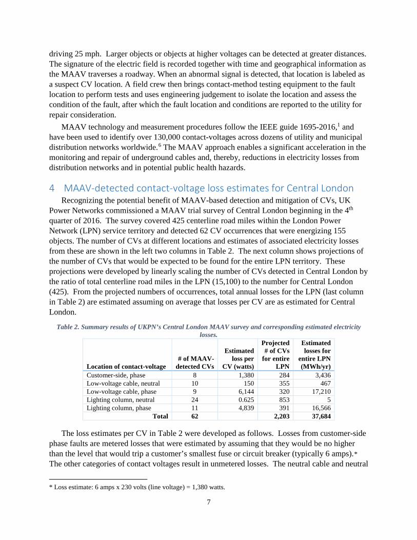
Power Networks commissioned a MAAV trial survey of Central London beginning in the 4th quarter of 2016. The survey covered 425 centerline road miles within the London Power Network (LPN) service territory and detected 62 CV occurrences that were energizing 155 objects. The number of CVs at different locations and estimates of associated electricity losses from these are shown in the left two columns in Table 2. The next column shows projections of the number of CVs that would be expected to be found for the entire LPN territory. These projections were developed by linearly scaling the number of CVs detected in Central London by the ratio of total centerline road miles in the LPN (15,100) to the number for Central London (425). From the projected numbers of occurrences, total annual losses for the LPN (last column in Table 2) are estimated assuming on average that losses per CV are as estimated for Central London.

Table 2. Summary results of UKPN’s Central London MAAV survey and corresponding estimated electricity losses.

Location of contact-voltage

# of MAAV- detected CVs

Estimated loss per

CV (watts)

Projected # of CVs

for entire LPN

Estimated losses for

entire LPN (MWh/yr)

Customer-side, phase 8 1,380 284 3,436 Low-voltage cable, neutral 10 150 355 467 Low-voltage cable, phase 9 6,144 320 17,210 Lighting column, neutral 24 0.625 853 5 Lighting column, phase 11 4,839 391 16,566

Total 62 2,203 37,684

The loss estimates per CV in Table 2 were developed as follows. Losses from customer-side phase faults are metered losses that were estimated by assuming that they would be no higher than the level that would trip a customer’s smallest fuse or circuit breaker (typically 6 amps).* The other categories of contact voltages result in unmetered losses. The neutral cable and neutral

* Loss estimate: 6 amps x 230 volts (line voltage) = 1,380 watts.

8

lighting column losses would be small and very small, respectively, and fixed values were assigned to these (Table 2). The largest losses are for phase-side cable and phase-side lighting column contact voltages.

These latter two categories of losses were estimated by first recognizing that the physical configuration of these types of CVs is analogous to that of earthing conductors widely used in electrical distribution systems. A faulted phase conductor in a buried cable often manifests as an unintentional connection between the phase conductor and its lead or aluminum sheath. At the time of installation, sheaths are continuous and would serve as a path for current if there were such unintentional contact. However, over time, there can be degradation that results in a discontinuous sheath. High fault currents in the sheath can contribute to this degradation, but regardless of the cause, the eventual result is that lengths of shield faulted to phase conductors become isolated and thereby energized at supply voltage level (nominally 230 volts). The intimate contact between such a buried sheath and the soil results in a high impedance fault to earth, much as with an earthing conductor. Similarly, a lighting column becomes energized when the supply phase conductor makes contact with the metal column, which itself is connected by a grounding wire to an earthing rod, effectively resulting in a high impedance fault to earth.

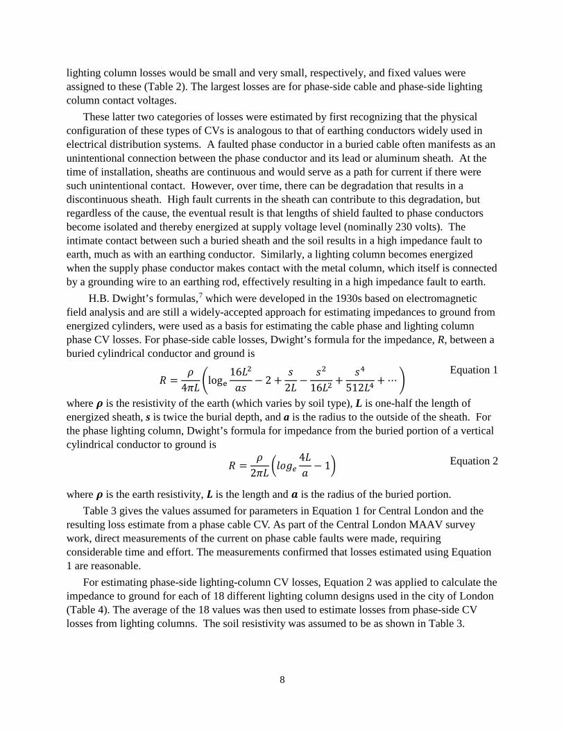
H.B. Dwight’s formulas,7 which were developed in the 1930s based on electromagnetic field analysis and are still a widely-accepted approach for estimating impedances to ground from energized cylinders, were used as a basis for estimating the cable phase and lighting column phase CV losses. For phase-side cable losses, Dwight’s formula for the impedance, R, between a buried cylindrical conductor and ground is

Equation 1 where 𝝆𝝆 is the resistivity of the earth (which varies by soil type), L is one-half the length of energized sheath, s is twice the burial depth, and a is the radius to the outside of the sheath. For the phase lighting column, Dwight’s formula for impedance from the buried portion of a vertical cylindrical conductor to ground is

Equation 2 where 𝝆𝝆 is the earth resistivity, 𝑳𝑳 is the length and 𝒂𝒂 is the radius of the buried portion.

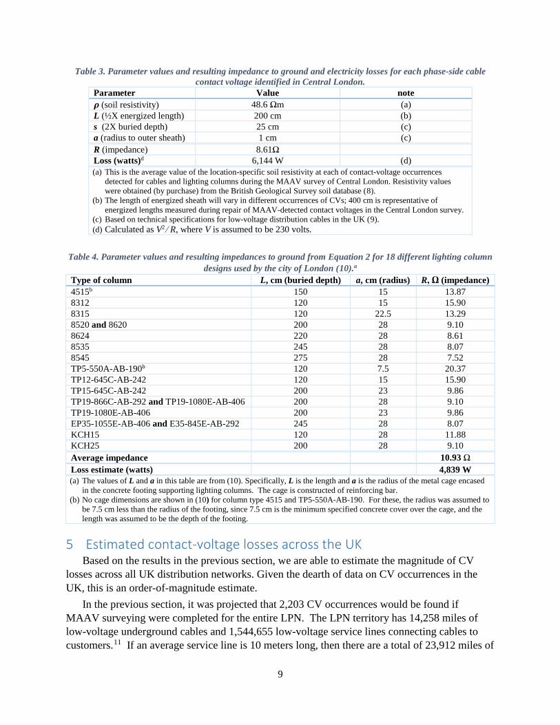
Table 3 gives the values assumed for parameters in Equation 1 for Central London and the resulting loss estimate from a phase cable CV. As part of the Central London MAAV survey work, direct measurements of the current on phase cable faults were made, requiring considerable time and effort. The measurements confirmed that losses estimated using Equation 1 are reasonable.

For estimating phase-side lighting-column CV losses, Equation 2 was applied to calculate the impedance to ground for each of 18 different lighting column designs used in the city of London (Table 4). The average of the 18 values was then used to estimate losses from phase-side CV losses from lighting columns. The soil resistivity was assumed to be as shown in Table 3.

𝑅𝑅 =𝜌𝜌

4𝜋𝜋𝜋𝜋loge

16𝜋𝜋2

𝑎𝑎𝑎𝑎− 2 +

𝑎𝑎2𝜋𝜋

−𝑎𝑎2

16𝜋𝜋2+

𝑎𝑎4

512𝜋𝜋4+ ⋯

𝑅𝑅 =𝜌𝜌

2𝜋𝜋𝜋𝜋𝑙𝑙𝑙𝑙𝑙𝑙𝑒𝑒

4𝜋𝜋𝑎𝑎− 1

9

Table 3. Parameter values and resulting impedance to ground and electricity losses for each phase-side cable contact voltage identified in Central London.

Parameter Value note 𝝆𝝆 (soil resistivity) 48.6 Ωm (a) L (½X energized length) 200 cm (b) s (2X buried depth) 25 cm (c) a (radius to outer sheath) 1 cm (c) R (impedance) 8.61Ω Loss (watts)d 6,144 W (d) (a) This is the average value of the location-specific soil resistivity at each of contact-voltage occurrences

detected for cables and lighting columns during the MAAV survey of Central London. Resistivity values were obtained (by purchase) from the British Geological Survey soil database (8).

(b) The length of energized sheath will vary in different occurrences of CVs; 400 cm is representative of energized lengths measured during repair of MAAV-detected contact voltages in the Central London survey.

(c) Based on technical specifications for low-voltage distribution cables in the UK (9). (d) Calculated as V2 ⁄ R, where V is assumed to be 230 volts.

Table 4. Parameter values and resulting impedances to ground from Equation 2 for 18 different lighting column

designs used by the city of London (10).a Type of column L, cm (buried depth) a, cm (radius) R, Ω (impedance) 4515b 150 15 13.87 8312 120 15 15.90 8315 120 22.5 13.29 8520 and 8620 200 28 9.10 8624 220 28 8.61 8535 245 28 8.07 8545 275 28 7.52 TP5-550A-AB-190b 120 7.5 20.37 TP12-645C-AB-242 120 15 15.90 TP15-645C-AB-242 200 23 9.86 TP19-866C-AB-292 and TP19-1080E-AB-406 200 28 9.10 TP19-1080E-AB-406 200 23 9.86 EP35-1055E-AB-406 and E35-845E-AB-292 245 28 8.07 KCH15 120 28 11.88 KCH25 200 28 9.10 Average impedance 10.93 Ω Loss estimate (watts) 4,839 W (a) The values of L and a in this table are from (10). Specifically, L is the length and a is the radius of the metal cage encased

in the concrete footing supporting lighting columns. The cage is constructed of reinforcing bar. (b) No cage dimensions are shown in (10) for column type 4515 and TP5-550A-AB-190. For these, the radius was assumed to

be 7.5 cm less than the radius of the footing, since 7.5 cm is the minimum specified concrete cover over the cage, and the length was assumed to be the depth of the footing.

5 Estimated contact-voltage losses across the UK Based on the results in the previous section, we are able to estimate the magnitude of CV

losses across all UK distribution networks. Given the dearth of data on CV occurrences in the UK, this is an order-of-magnitude estimate.

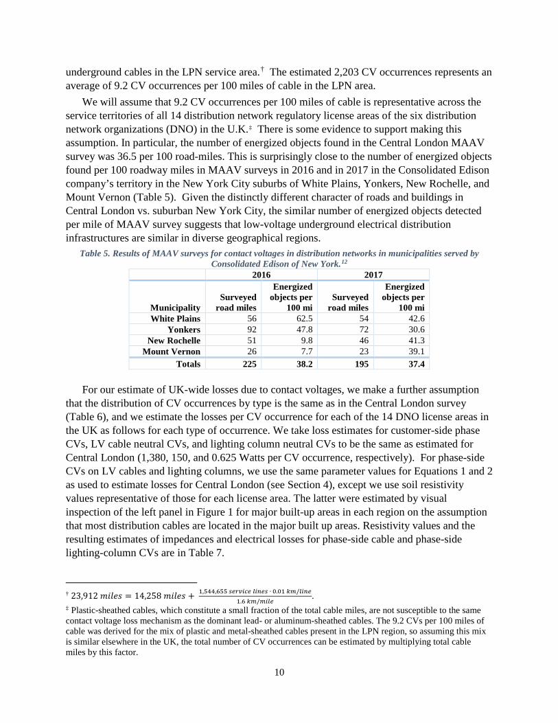
In the previous section, it was projected that 2,203 CV occurrences would be found if MAAV surveying were completed for the entire LPN. The LPN territory has 14,258 miles of low-voltage underground cables and 1,544,655 low-voltage service lines connecting cables to customers.11 If an average service line is 10 meters long, then there are a total of 23,912 miles of

10

underground cables in the LPN service area.† The estimated 2,203 CV occurrences represents an average of 9.2 CV occurrences per 100 miles of cable in the LPN area.

We will assume that 9.2 CV occurrences per 100 miles of cable is representative across the service territories of all 14 distribution network regulatory license areas of the six distribution network organizations (DNO) in the U.K.‡ There is some evidence to support making this assumption. In particular, the number of energized objects found in the Central London MAAV survey was 36.5 per 100 road-miles. This is surprisingly close to the number of energized objects found per 100 roadway miles in MAAV surveys in 2016 and in 2017 in the Consolidated Edison company’s territory in the New York City suburbs of White Plains, Yonkers, New Rochelle, and Mount Vernon (Table 5). Given the distinctly different character of roads and buildings in Central London vs. suburban New York City, the similar number of energized objects detected per mile of MAAV survey suggests that low-voltage underground electrical distribution infrastructures are similar in diverse geographical regions.

Table 5. Results of MAAV surveys for contact voltages in distribution networks in municipalities served by Consolidated Edison of New York.12

2016 2017

Municipality Surveyed

road miles

Energized objects per

100 mi Surveyed

road miles

Energized objects per

100 mi White Plains 56 62.5 54 42.6

Yonkers 92 47.8 72 30.6 New Rochelle 51 9.8 46 41.3

Mount Vernon 26 7.7 23 39.1 Totals 225 38.2 195 37.4

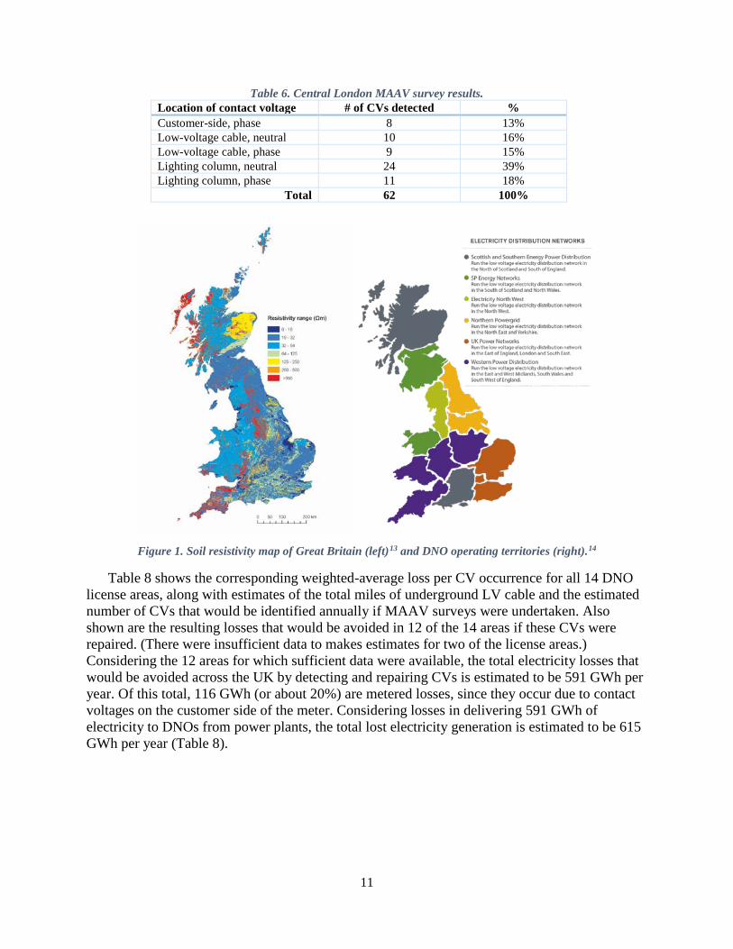
For our estimate of UK-wide losses due to contact voltages, we make a further assumption

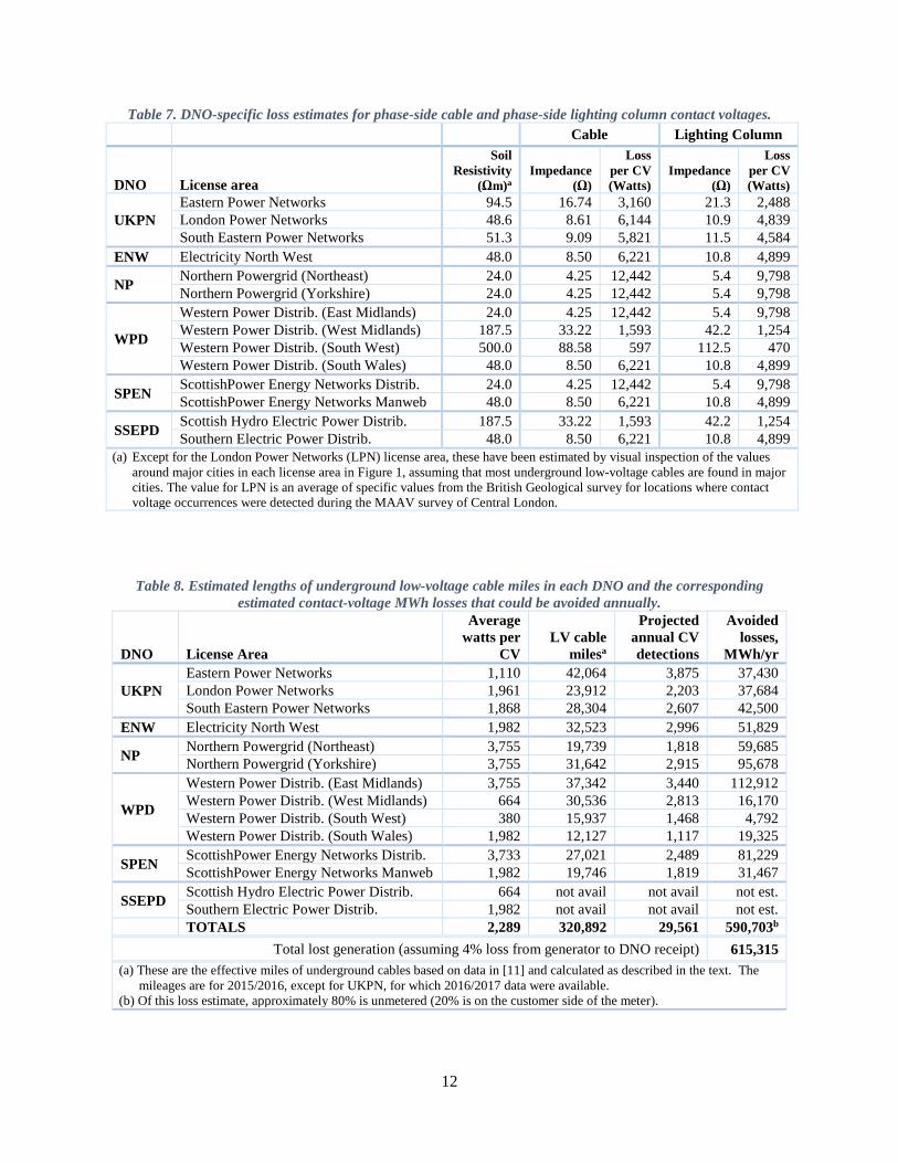
that the distribution of CV occurrences by type is the same as in the Central London survey (Table 6), and we estimate the losses per CV occurrence for each of the 14 DNO license areas in the UK as follows for each type of occurrence. We take loss estimates for customer-side phase CVs, LV cable neutral CVs, and lighting column neutral CVs to be the same as estimated for Central London (1,380, 150, and 0.625 Watts per CV occurrence, respectively). For phase-side CVs on LV cables and lighting columns, we use the same parameter values for Equations 1 and 2 as used to estimate losses for Central London (see Section 4), except we use soil resistivity values representative of those for each license area. The latter were estimated by visual inspection of the left panel in Figure 1 for major built-up areas in each region on the assumption that most distribution cables are located in the major built up areas. Resistivity values and the resulting estimates of impedances and electrical losses for phase-side cable and phase-side lighting-column CVs are in Table 7.

† 23,912 𝑚𝑚𝑚𝑚𝑙𝑙𝑚𝑚𝑎𝑎 = 14,258 𝑚𝑚𝑚𝑚𝑙𝑙𝑚𝑚𝑎𝑎 + 1,544,655 𝑠𝑠𝑒𝑒𝑠𝑠𝑠𝑠𝑠𝑠𝑠𝑠𝑒𝑒 𝑙𝑙𝑠𝑠𝑙𝑙𝑒𝑒𝑠𝑠 ∙ 0.01 𝑘𝑘𝑘𝑘/𝑙𝑙𝑠𝑠𝑙𝑙𝑒𝑒

1.6 𝑘𝑘𝑘𝑘/𝑘𝑘𝑠𝑠𝑙𝑙𝑒𝑒.

‡ Plastic-sheathed cables, which constitute a small fraction of the total cable miles, are not susceptible to the same contact voltage loss mechanism as the dominant lead- or aluminum-sheathed cables. The 9.2 CVs per 100 miles of cable was derived for the mix of plastic and metal-sheathed cables present in the LPN region, so assuming this mix is similar elsewhere in the UK, the total number of CV occurrences can be estimated by multiplying total cable miles by this factor.

11

Table 6. Central London MAAV survey results. Location of contact voltage # of CVs detected % Customer-side, phase 8 13% Low-voltage cable, neutral 10 16% Low-voltage cable, phase 9 15% Lighting column, neutral 24 39% Lighting column, phase 11 18%

Total 62 100%

Figure 1. Soil resistivity map of Great Britain (left)13 and DNO operating territories (right).14

Table 8 shows the corresponding weighted-average loss per CV occurrence for all 14 DNO license areas, along with estimates of the total miles of underground LV cable and the estimated number of CVs that would be identified annually if MAAV surveys were undertaken. Also shown are the resulting losses that would be avoided in 12 of the 14 areas if these CVs were repaired. (There were insufficient data to makes estimates for two of the license areas.) Considering the 12 areas for which sufficient data were available, the total electricity losses that would be avoided across the UK by detecting and repairing CVs is estimated to be 591 GWh per year. Of this total, 116 GWh (or about 20%) are metered losses, since they occur due to contact voltages on the customer side of the meter. Considering losses in delivering 591 GWh of electricity to DNOs from power plants, the total lost electricity generation is estimated to be 615 GWh per year (Table 8).

12

Table 7. DNO-specific loss estimates for phase-side cable and phase-side lighting column contact voltages. Cable Lighting Column

DNO License area

Soil Resistivity

(Ωm)a Impedance

(Ω)

Loss per CV (Watts)

Impedance (Ω)

Loss per CV (Watts)

UKPN Eastern Power Networks 94.5 16.74 3,160 21.3 2,488 London Power Networks 48.6 8.61 6,144 10.9 4,839 South Eastern Power Networks 51.3 9.09 5,821 11.5 4,584

ENW Electricity North West 48.0 8.50 6,221 10.8 4,899

NP Northern Powergrid (Northeast) 24.0 4.25 12,442 5.4 9,798 Northern Powergrid (Yorkshire) 24.0 4.25 12,442 5.4 9,798

WPD

Western Power Distrib. (East Midlands) 24.0 4.25 12,442 5.4 9,798 Western Power Distrib. (West Midlands) 187.5 33.22 1,593 42.2 1,254 Western Power Distrib. (South West) 500.0 88.58 597 112.5 470 Western Power Distrib. (South Wales) 48.0 8.50 6,221 10.8 4,899

SPEN ScottishPower Energy Networks Distrib. 24.0 4.25 12,442 5.4 9,798 ScottishPower Energy Networks Manweb 48.0 8.50 6,221 10.8 4,899

SSEPD Scottish Hydro Electric Power Distrib. 187.5 33.22 1,593 42.2 1,254 Southern Electric Power Distrib. 48.0 8.50 6,221 10.8 4,899

(a) Except for the London Power Networks (LPN) license area, these have been estimated by visual inspection of the values around major cities in each license area in Figure 1, assuming that most underground low-voltage cables are found in major cities. The value for LPN is an average of specific values from the British Geological survey for locations where contact voltage occurrences were detected during the MAAV survey of Central London.

Table 8. Estimated lengths of underground low-voltage cable miles in each DNO and the corresponding estimated contact-voltage MWh losses that could be avoided annually.

DNO License Area

Average watts per

CV LV cable

milesa

Projected annual CV detections

Avoided losses,

MWh/yr

UKPN Eastern Power Networks 1,110 42,064 3,875 37,430 London Power Networks 1,961 23,912 2,203 37,684 South Eastern Power Networks 1,868 28,304 2,607 42,500

ENW Electricity North West 1,982 32,523 2,996 51,829

NP Northern Powergrid (Northeast) 3,755 19,739 1,818 59,685 Northern Powergrid (Yorkshire) 3,755 31,642 2,915 95,678

WPD

Western Power Distrib. (East Midlands) 3,755 37,342 3,440 112,912 Western Power Distrib. (West Midlands) 664 30,536 2,813 16,170 Western Power Distrib. (South West) 380 15,937 1,468 4,792 Western Power Distrib. (South Wales) 1,982 12,127 1,117 19,325

SPEN ScottishPower Energy Networks Distrib. 3,733 27,021 2,489 81,229 ScottishPower Energy Networks Manweb 1,982 19,746 1,819 31,467

SSEPD Scottish Hydro Electric Power Distrib. 664 not avail not avail not est. Southern Electric Power Distrib. 1,982 not avail not avail not est.

TOTALS 2,289 320,892 29,561 590,703b Total lost generation (assuming 4% loss from generator to DNO receipt) 615,315

(a) These are the effective miles of underground cables based on data in [11] and calculated as described in the text. The mileages are for 2015/2016, except for UKPN, for which 2016/2017 data were available.

(b) Of this loss estimate, approximately 80% is unmetered (20% is on the customer side of the meter).

13

6 Contact-voltage loss estimate in perspective The estimated unmetered CV losses on UK distribution networks (474 GWh/year) represent

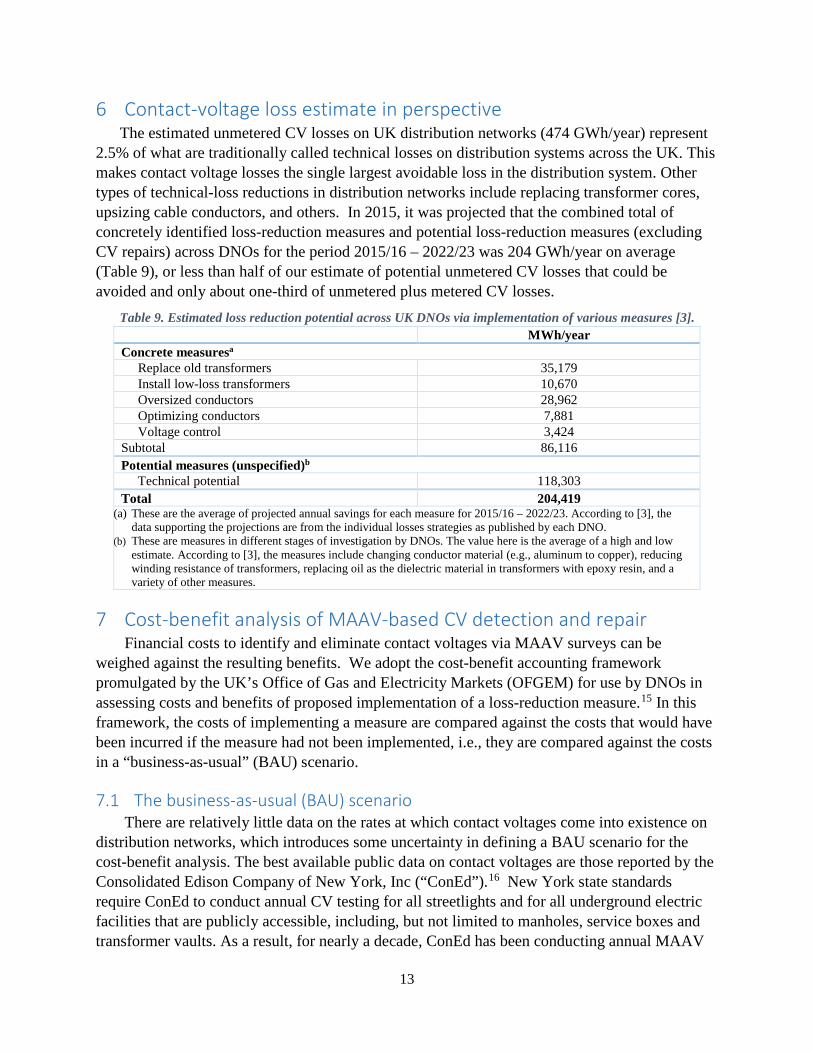
2.5% of what are traditionally called technical losses on distribution systems across the UK. This makes contact voltage losses the single largest avoidable loss in the distribution system. Other types of technical-loss reductions in distribution networks include replacing transformer cores, upsizing cable conductors, and others. In 2015, it was projected that the combined total of concretely identified loss-reduction measures and potential loss-reduction measures (excluding CV repairs) across DNOs for the period 2015/16 – 2022/23 was 204 GWh/year on average (Table 9), or less than half of our estimate of potential unmetered CV losses that could be avoided and only about one-third of unmetered plus metered CV losses.

Table 9. Estimated loss reduction potential across UK DNOs via implementation of various measures [3]. MWh/year

Concrete measuresa Replace old transformers 35,179 Install low-loss transformers 10,670 Oversized conductors 28,962 Optimizing conductors 7,881 Voltage control 3,424 Subtotal 86,116 Potential measures (unspecified)b Technical potential 118,303 Total 204,419

(a) These are the average of projected annual savings for each measure for 2015/16 – 2022/23. According to [3], the data supporting the projections are from the individual losses strategies as published by each DNO.

(b) These are measures in different stages of investigation by DNOs. The value here is the average of a high and low estimate. According to [3], the measures include changing conductor material (e.g., aluminum to copper), reducing winding resistance of transformers, replacing oil as the dielectric material in transformers with epoxy resin, and a variety of other measures.

7 Cost-benefit analysis of MAAV-based CV detection and repair Financial costs to identify and eliminate contact voltages via MAAV surveys can be

weighed against the resulting benefits. We adopt the cost-benefit accounting framework promulgated by the UK’s Office of Gas and Electricity Markets (OFGEM) for use by DNOs in assessing costs and benefits of proposed implementation of a loss-reduction measure.15 In this framework, the costs of implementing a measure are compared against the costs that would have been incurred if the measure had not been implemented, i.e., they are compared against the costs in a “business-as-usual” (BAU) scenario.

7.1 The business-as-usual (BAU) scenario There are relatively little data on the rates at which contact voltages come into existence on

distribution networks, which introduces some uncertainty in defining a BAU scenario for the cost-benefit analysis. The best available public data on contact voltages are those reported by the Consolidated Edison Company of New York, Inc (“ConEd”).16 New York state standards require ConEd to conduct annual CV testing for all streetlights and for all underground electric facilities that are publicly accessible, including, but not limited to manholes, service boxes and transformer vaults. As a result, for nearly a decade, ConEd has been conducting annual MAAV

14

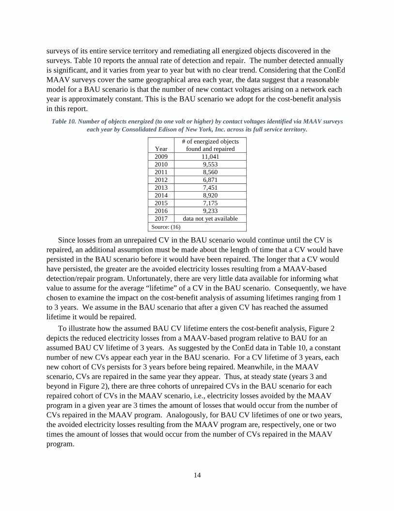
surveys of its entire service territory and remediating all energized objects discovered in the surveys. Table 10 reports the annual rate of detection and repair. The number detected annually is significant, and it varies from year to year but with no clear trend. Considering that the ConEd MAAV surveys cover the same geographical area each year, the data suggest that a reasonable model for a BAU scenario is that the number of new contact voltages arising on a network each year is approximately constant. This is the BAU scenario we adopt for the cost-benefit analysis in this report.

Table 10. Number of objects energized (to one volt or higher) by contact voltages identified via MAAV surveys each year by Consolidated Edison of New York, Inc. across its full service territory.

Year # of energized objects

found and repaired 2009 11,041 2010 9,553 2011 8,560 2012 6,871 2013 7,451 2014 8,920 2015 7,175 2016 9,233 2017 data not yet available

Source: (16)

Since losses from an unrepaired CV in the BAU scenario would continue until the CV is repaired, an additional assumption must be made about the length of time that a CV would have persisted in the BAU scenario before it would have been repaired. The longer that a CV would have persisted, the greater are the avoided electricity losses resulting from a MAAV-based detection/repair program. Unfortunately, there are very little data available for informing what value to assume for the average “lifetime” of a CV in the BAU scenario. Consequently, we have chosen to examine the impact on the cost-benefit analysis of assuming lifetimes ranging from 1 to 3 years. We assume in the BAU scenario that after a given CV has reached the assumed lifetime it would be repaired.

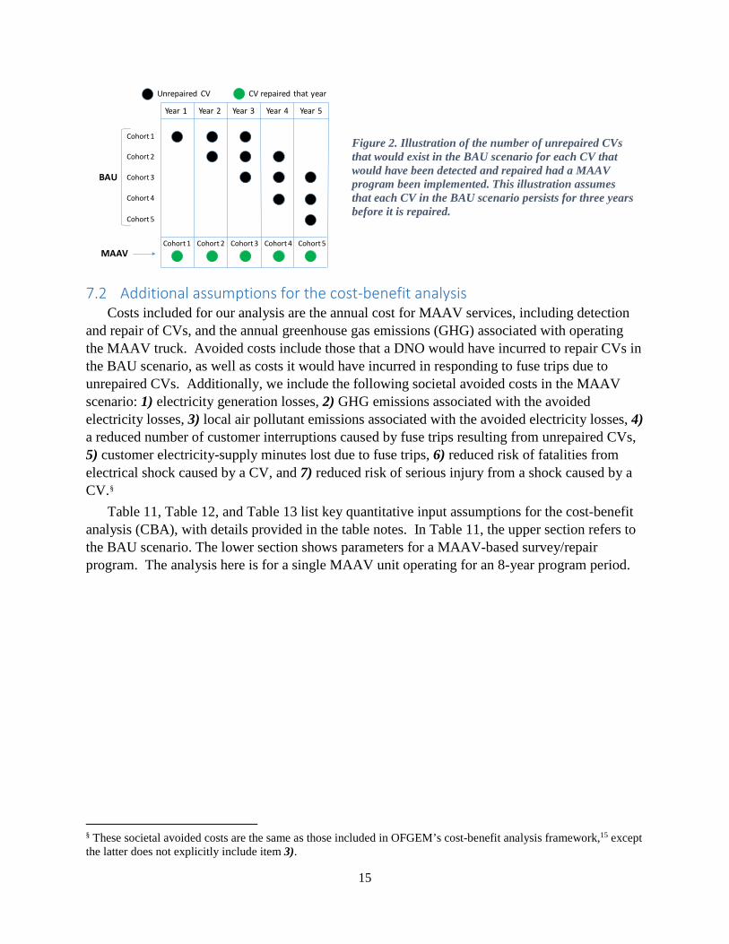
To illustrate how the assumed BAU CV lifetime enters the cost-benefit analysis, Figure 2 depicts the reduced electricity losses from a MAAV-based program relative to BAU for an assumed BAU CV lifetime of 3 years. As suggested by the ConEd data in Table 10, a constant number of new CVs appear each year in the BAU scenario. For a CV lifetime of 3 years, each new cohort of CVs persists for 3 years before being repaired. Meanwhile, in the MAAV scenario, CVs are repaired in the same year they appear. Thus, at steady state (years 3 and beyond in Figure 2), there are three cohorts of unrepaired CVs in the BAU scenario for each repaired cohort of CVs in the MAAV scenario, i.e., electricity losses avoided by the MAAV program in a given year are 3 times the amount of losses that would occur from the number of CVs repaired in the MAAV program. Analogously, for BAU CV lifetimes of one or two years, the avoided electricity losses resulting from the MAAV program are, respectively, one or two times the amount of losses that would occur from the number of CVs repaired in the MAAV program.

15

Figure 2. Illustration of the number of unrepaired CVs that would exist in the BAU scenario for each CV that would have been detected and repaired had a MAAV program been implemented. This illustration assumes that each CV in the BAU scenario persists for three years before it is repaired.

7.2 Additional assumptions for the cost-benefit analysis Costs included for our analysis are the annual cost for MAAV services, including detection

and repair of CVs, and the annual greenhouse gas emissions (GHG) associated with operating the MAAV truck. Avoided costs include those that a DNO would have incurred to repair CVs in the BAU scenario, as well as costs it would have incurred in responding to fuse trips due to unrepaired CVs. Additionally, we include the following societal avoided costs in the MAAV scenario: 1) electricity generation losses, 2) GHG emissions associated with the avoided electricity losses, 3) local air pollutant emissions associated with the avoided electricity losses, 4) a reduced number of customer interruptions caused by fuse trips resulting from unrepaired CVs, 5) customer electricity-supply minutes lost due to fuse trips, 6) reduced risk of fatalities from electrical shock caused by a CV, and 7) reduced risk of serious injury from a shock caused by a CV.§

Table 11, Table 12, and Table 13 list key quantitative input assumptions for the cost-benefit analysis (CBA), with details provided in the table notes. In Table 11, the upper section refers to the BAU scenario. The lower section shows parameters for a MAAV-based survey/repair program. The analysis here is for a single MAAV unit operating for an 8-year program period.

§ These societal avoided costs are the same as those included in OFGEM’s cost-benefit analysis framework,15 except the latter does not explicitly include item 3).

BAU

Year 1 Year 2 Year 3 Year 4 Year 5

Cohort 1

Cohort 2

Cohort 3

Cohort 4

MAAVCohort 1 Cohort 2 Cohort 3 Cohort 4 Cohort 5

Cohort 5

Unrepaired CV CV repaired that year

16

Table 11. Input assumptions for cost-benefit analysis. Business-as-usual, i.e., with no MAAV program

Average lost electricity generationa 14,090 MWh/year Number of fuse trips per CVb 3 per year Customers interrupted per fuse operationc 10 Customer minutes lost per fuse operationc 60 Lifetime that a CV persists before it is repairedd range: 1 – 3 years

With MAAV survey/repair program Number of MAAV-detected phase-side cable CVe 115 per truck-year Reduced risk of fatality due to shock from CVf 10% Reduced risk of major injury due to shock from CVf 15% CO2 emissions from one MAAV truck 6 tCO2e/year

(a) This is the amount of electricity estimated to be lost due to contact voltages equivalent to those that would be identified by a single MAAV truck surveying continuously for one year. The estimate was derived as follows. A MAAV survey of the full LPN license area would identify contact voltages that collectively result in 37,684 MWh per year of losses (Table 2). If MAAV trucks were to operate 24 hours per day for a year (excluding bank holidays), it is estimated that 2.786 trucks would be required to complete a full survey of the LPN. On this basis, the electricity losses associated with CVs detected by a single truck would be 37,684/2.786 = 13,526 MWh/year. Guidance from OFGEM for cost-benefit analysis of proposed improvements to distribution networks [15] indicates that 4% losses in moving the electricity from the point of generation to the point of loss in the distribution system should be included: 13,526 / (1 – 0.04) = 14,090 MWh/year.

(b) UKPN estimate. Unrepaired CVs can cause fuses on the network to trip, necessitating a reset. Under BAU operation it is estimated that a fuse trip occurs on average 3 times per year for each contact voltage.

(c) UKPN estimate. (d) See discussion in text. (e) Phase cable contact voltage faults, if not avoided by a MAAV program, would have resulted in BAU costs associated with

fuse trips, customer interruptions, customer minutes lost, and eventually detection and repair. A total of 320 occurrences of phase cable CVs are projected for a one-year survey covering the full LPN area (Table 2). As indicated in table note (a) above, an estimated 2.79 MAAV trucks would be required to accomplish a full LPN survey in one year. Thus, the expectation is that one MAAV unit would detect 320/2.79 = 115 phase cable contact voltages.

(f) The risks of fatalities and of major injuries are assumed to be reduced by 10% and 15% when a MAAV program is in place.

Table 12. Valuations of costs and benefits associated with MAAV detection and repair of contact voltages.a Costs incurred with MAAV program CV detection and repair for an 8-year programb £2.39 million per year GHG emissions from operating MAAV see Table 13 for emissions costs Costs avoided Repair of contact voltagesb £ 0.46 million per year Responses to fuse operationsb £ 250 per fuse operation Societal avoided costs Electricity generationc £ 48.42 per MWh GHG emissions from electricity generation see Table 13 for emissions costs Air pollution from electricity generation see Table 13 for emissions costs Customer interruptions (CI)c £ 15.44 per CI Customer-minutes lost (CML)c £ 0.38 per CML Fatality due to CV shockd £ 1.79 million per fatality Risk of a major injuryd £ 27,488 per major injury Financial parameter assumptions Weighted-average cost of capital (real) 4.08%/year DNO asset capitalization ratec 85% Capital depreciationc Straight-line, 45 years (a) All monetary values are given in 2013 £. (b) UKPN estimate. (c) OFGEM guidance for cost-benefit analysis [15]. (d) Source: OFGEM guidance [15], based on Health and Safety Executive guidelines [17]. The corresponding cost avoided by

the MAAV program is this value multiplied by the assumed percentage risk reduction shown in Table 11.

17

Table 13. Greenhouse gas (GHG) emission trading prices, air pollution damage costs, and grid electricity GHG emissions recommended by the UK government (BEIS) and by OFGEM for use in appraisals. The analysis in

this report uses the OFGEM values where available.

GHG Trading Prices (2012/2013 £/tCO2e)

Air pollution damages, generation

based (£/MWh) Grid-average GHG emissions,

generation-based (tCO2e/MWh) BEISa,b OFGEMc BEISa,b BEISa OFGEMc Low Central High 2017 0.0 4.1 4.1 7.67 0.157 0.265 0.488 2018 0.0 4.1 4.4 8.16 0.160 0.235 0.474 2019 0.0 4.2 6.9 8.68 0.163 0.224 0.459 2020 0.0 4.4 8.8 9.24 0.166 0.198 0.445 2021 3.7 11.4 19.1 16.49 0.170 0.194 0.430 2022 7.4 18.4 29.4 23.74 0.173 0.161 0.416 2023 11.2 25.4 39.7 30.98 0.177 0.171 0.401 2024 14.9 32.4 50.0 38.23 0.180 0.184 0.387 2025 18.6 39.4 60.3 45.48 0.184 0.174 0.372 2026 22.3 46.5 70.6 52.73 0.187 0.153 0.358 2027 26.1 53.5 80.8 59.98 0.191 0.143 0.343 2028 29.8 60.5 91.1 67.23 0.195 0.118 0.329 2029 33.5 67.5 101.4 74.48 0.199 0.103 0.314 2030 37.2 74.5 111.7 81.73 0.203 0.107 0.300

(a) From [18]. (b) Originally given in 2016 £, converted to 2012/2013 £ using UK GDP deflators [19]. (c) From [15].

7.3 Results Figure 3 shows discounted annual costs and benefits for an 8-year MAAV-based CV

detection and repair program starting in 2018, assuming that without the program CVs would have persisted for 1 year before being repaired. By far the largest benefit each year is avoided electricity losses. Reduced risks of fatalities are a distant second largest benefit. The other benefits are each relatively small individually, but the avoided CO2 emissions grows to become the second largest benefit in the 7th and 8th years of the program.

Figure 3. Discounted annual costs and benefits (left axis) and cumulative discounted net benefits (right axis) for an 8-year MAAV-based CV detection and repair program, assuming CVs persist for 1 year in the BAU scenario.

In the OFGEM cost-benefit analysis framework used here, the value of a loss-reduction investment is judged by the cumulative discounted net benefit resulting from its implementation.

-3.0

-2.0

-1.0

0.0

1.0

2.0

3.0

4.0

5.0

(750)

(500)

(250)

0

250

500

750

1,000

1,250

2018 2019 2020 2021 2022 2023 2024 2025

Cum

ulat

ive

Disc

ount

ed N

et B

enef

itsM

illion

£ (2

013

£)

Disc

ount

ed A

nnua

l Cos

ts/B

enef

itsTh

ousa

nd £

(201

3 £)

Reduced risk of major injuries

Reduced air pollution damages

Reduced risk of fatalities

Reduced customer interruptions

Reduced customer-minutes lost

Reduced CO2 emissions

Reduced MWh lost

Cost of capital

Depreciation

Expensed capital

Net annual benefit

Cumulative net benefits

18

The cumulative discounted net benefit for the MAAV program grows from £0.77 million in the first year to £3.65 million at the end of the program (year 8), as shown in Figure 3. If the CV lifetime assumed for the BAU scenario were 2 years instead of one, the cumulative discounted net benefit in year 8 grows to £10.6 million, and if a BAU CV lifetime of 3 years were assumed, the net benefit grows to £17.5 million (Figure 4).

Figure 4. Discounted annual costs and benefits for an 8-year MAAV-based CV detection and repair program

with different assuming CV lifetimes in the BAU scenario.

8 Conclusions and some reflections Based on the analysis in this report, contact-voltage losses are one of the single largest

avoidable loss of electricity from distribution networks in the UK. Our order-of-magnitude estimate is that they account for about 2.5% of unmetered distribution system losses in the category traditionally defined as technical losses. By comparison, upgrades to transformers, upsizing of conductors, and other measures might collectively reduce technical losses by only about 1%. Moreover, if such losses are reduced by over-sizing components, then the upgraded assets will be under-utilized until load catches up, at which point the losses return. Given that considerable capital investment may be required for such upgrades, and may include retiring existing equipment before the end of its useful life, are the ratio of benefits to costs for such measures as positive as our analysis suggests they are for eliminating CV losses? Detailed cost-benefit comparisons, which are beyond the scope of this work, are needed to answer this question.

Finally, it is of interest to consider how the future evolution of the electricity grid might impact the frequency of contact-voltage losses. For example, what might be the impact in a future low-carbon grid that includes massive distributed renewable generation? It is difficult to be more than speculative in answering such questions. However, it is safe to say that where existing distribution cables are no longer needed and are taken out of service, contact-voltage losses would diminish correspondingly. On the other hand, unlike some technical losses, such as transformer losses, contact-voltage losses are independent of power flow: they depend only on the line voltage and the impedance to ground. Thus, to the extent that line power flows diminish, e.g., due to greater distributed self-generation and associated self-consumption, technical losses

0

2

4

6

8

10

12

14

16

18

2018 2019 2020 2021 2022 2023 2024 2025

Cum

ulat

ive

disc

ount

ed n

et b

enef

it(m

illio

n 20

13 £

)

3 years2 years1 year (see Figure 3)

CV lifetime in BAU scenario

19

other than CV losses will diminish, and, ceteris paribus, contact-voltage losses will become a larger fraction of total losses.

9 References 1. Transmission and Distribution Committee, “IEEE Guide to Understanding, Diagnosing, and Mitigating Stray

and Contact Voltage,” IEEE Standard 1695-2016, Power and Energy Society of the Institute of Electrical and Electronics Engineers, New York, NY, 2016.

2. UK Department for Business, Energy and Industrial Strategy, Digest of UK Energy Statistics (DUKES): electricity,” 27 July 2017.

3. UK Office of Gas and Electricity Markets, “Energy Efficiency Directive: An assessment of the energy efficiency potential of Great Britain’s gas and electricity infrastructure,” OFGEM, 16 June 2015.

4. UK Office of Gas and Electricity Markets, “Electricity distribution losses: a consultation document,” OFGEM, January 2003.

5. Wright, J.L., “Surveying for Electrical Losses,” Electric Energy T&D Magazine, Jan/Feb 2016 issue.

6. Wright, J.L., “Losses on the low voltage underground cable network due to contact voltage,” presentation at UK Power Networks Losses Stakeholder Event, Imperial College, Kensington, London, 6 July 2017.

7. Dwight, H.B., “Calculation of Resistances to Ground,” Electrical Engineering, 55(12): 1319 – 1328, Dec. 1936.

8. Entwisle, D.C., White, J.C., Busby, J.P., Lawley, R.S., and Cooke, I.L., “Electrical Resistivity Model of Great Britain: User Guide,” British Geological Survey Open Report, OR/14/030, 2014.

9. British Standards Institution, “Specification for Impregnated paper-insulated lead or lead alloy sheathed electric cables of rated voltages up to and including 33 000 V,” BS 6480:1988, Incorporating Amendments Nos. 1 and 2 and Corrigendum No. 1), 21 Feburary, 2003.

10. City of London, “Supplemental Standards for Traffic Signal and Street Lighting,” STS 5.02, Nov. 3, 2017.

11. DNO-Shared Asset Database, provided by UKPN to the authors.

12. Consolidated Edison Co. of New York, Inc., "Report on Mobile Testing for Contact Voltage Performed Outside of New York City," 10-E-0271, 24 July 2017.

13. CP17/050 British Geological Survey © NERC [2017]. Permission to reprint this map provided to Eric Larson by the Natural Environmental Research Council as represented by the British Geological Society, 14 Aug 2017.

14. Source: UK Office of Gas and Electricity Markets (OFGEM) website.

15. OFGEM’s spreadsheet template for cost-benefit analysis (filename: Template CBA RIIO ED1 v4.xls) provided to the authors by UKPN.

16. Consolidated Edison Co. of New York, Inc., “Contact Voltage Test and Facility Inspection Annual Report,” filed each February pursuant to the requirements of the NY State Public Service Commission’s Electric Safety Standards issued in Case 04-M-0159 (Proceeding on the Motion of the Commission to Examine the Safety of Electric Transmission and Distribution Systems). All published reports are available here.

17. Health and Safety Executive, “Cost-Benefit Analysis (CBA) Checklist,” website, Government of the UK, accessed 13 Oct 2017.

18. Department for Business, Energy and Industrial Strategy,“Green Book supplementary guidance: valuation of energy use and greenhouse gas emissions for appraisal,” UK Government, 15 March 2017 (URL).

19. HM Treasury, GDP deflators at market prices, and money GDP September 2017 (Quarterly National Accounts, September 2017), 2 October 2017. (accessed 31 October 2017)