Analysis of Count Data

Goodness of fit Formulas and models for two-way

tables- tests for independence- tests of homogeneity

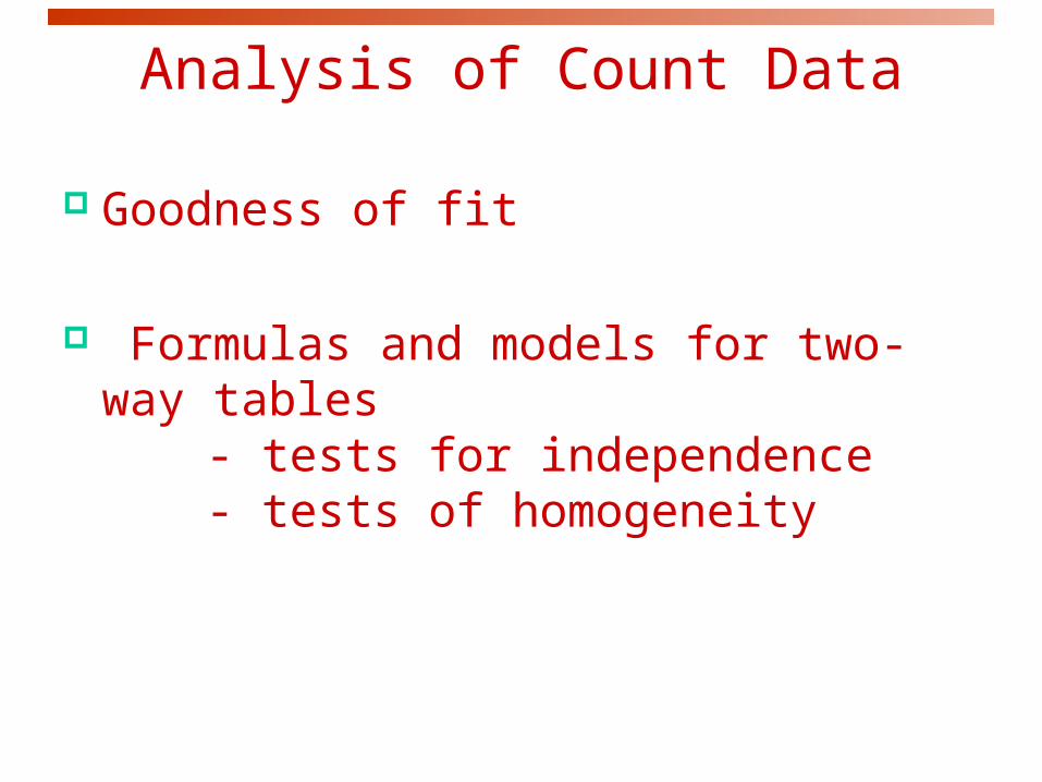
A study of 667 drivers who were using a cell phone when they were involved

in a collision on a weekday examined the relationship between these

accidents and the day of the week.

Example 1: Car accidents and day of the week

Are the accidents equally likely to occur on any day of the working week?

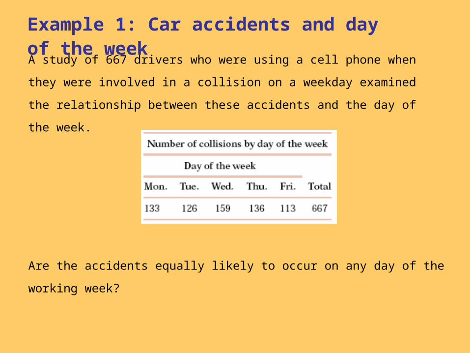
Example 2: M & M Colors

Mars, Inc. periodically changes the M&M (milk chocolate) color proportions. Last year the proportions were:

yellow 20%; red 20%, orange, blue, green 10% each; brown 30% In a recent bag of 106 M&M’s I had the following numbers of each

color:

Is this evidence that Mars, Inc. has changed the color distribution of M&M’s?

Yellow Red Orange Blue Green Brown

29 (27.4%) 23 (21.7%) 12 (11.3%) 14 (13.2%) 8 (7.5%) 20 (18.9%)

Example 3: Are successful people more likely to be born under some astrological signs than others? 256 executives of Fortune

400 companies have birthday signs shown at the right.

There is some variation in the number of births per sign, and there are more Pisces.

Can we claim that successful people are more likely to be born under some signs than others?

Births Sign

23 Aries

20 Taurus

18 Gemini

23 Cancer

20 Leo

19 Virgo

18 Libra

21 Scorpio

19 Sagittarius

22 Capricorn

24 Aquarius

29 Pisces

To answer these questions we use the chi-square goodness of fit test

Data for n observations on a categorical variable with k possible

outcomes are summarized as observed counts, n1, n2, . . . , nk in k cells.

2 hypotheses: null hypothesis H0 and alternative hypothesis HA

H0 specifies probabilities p1, p2, . . . , pk for the possible outcomes.

HA states that the probabilities are different from those in H0

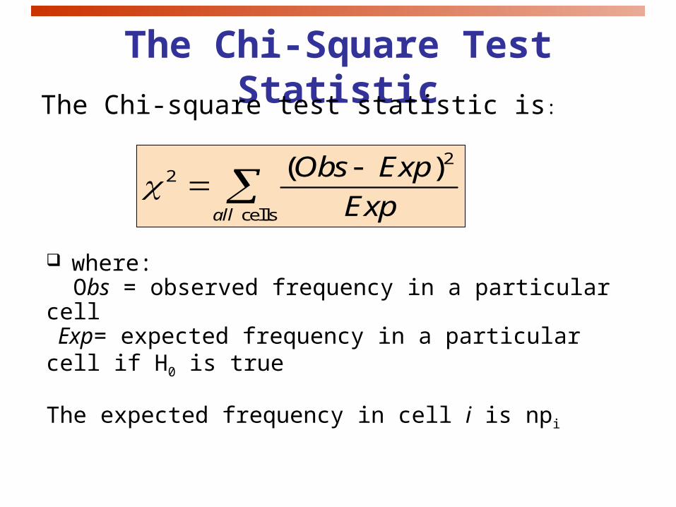
The Chi-Square Test StatisticThe Chi-square test statistic is:

22

cells

( )

all

Obs Exp

Exp

where: Obs = observed frequency in a particular cell Exp= expected frequency in a particular cell if H0 is true

The expected frequency in cell i is npi

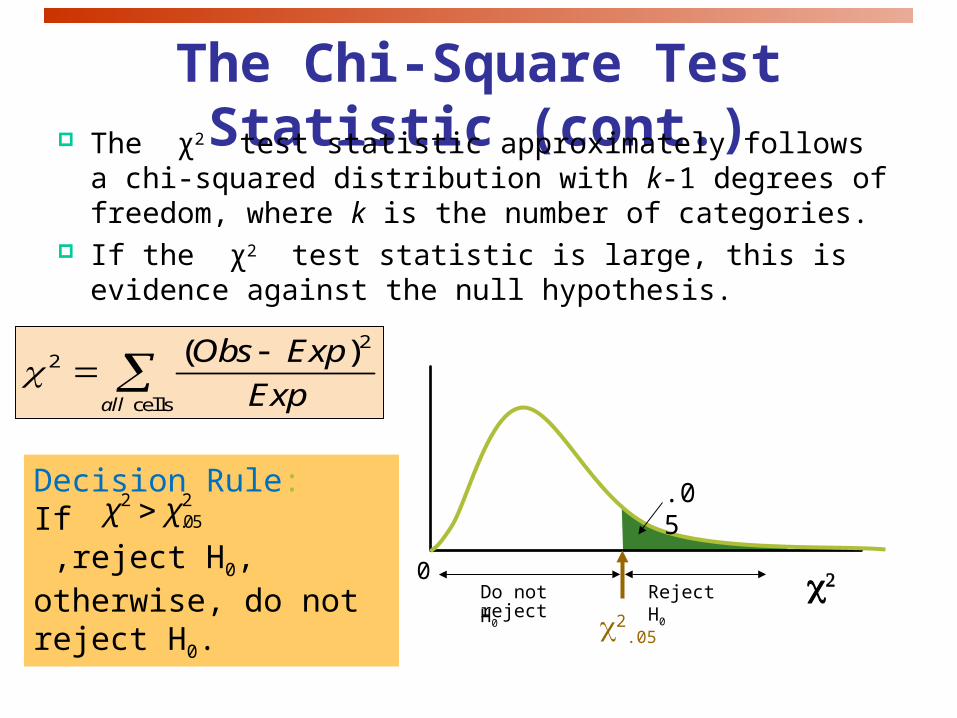
The Chi-Square Test Statistic (cont.) The χ2 test statistic approximately follows a chi-squared

distribution with k-1 degrees of freedom, where k is the number of categories.

If the χ2 test statistic is large, this is evidence against the null hypothesis.

Decision Rule:If ,reject H0, otherwise, do not reject H0.

2 2.05χ χ

2.05

0

.05

Reject H0Do not reject H0

22

cells

( )

all

Obs Exp

Exp

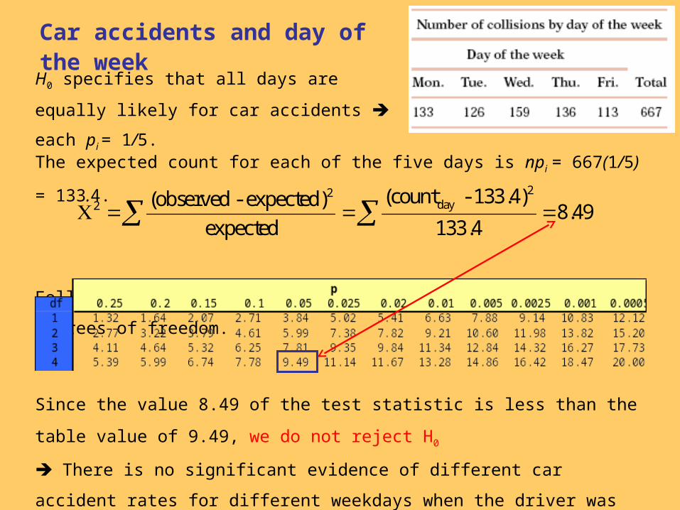
H0 specifies that all days are equally likely for

car accidents each pi = 1/5.

Car accidents and day of the week

The expected count for each of the five days is npi = 667(1/5) = 133.4.

Following the chi-square distribution with 5 − 1 = 4 degrees of freedom.

22day2 (count - 133.4)(observed - expected)

8.49expected 133.4

Since the value 8.49 of the test statistic is less than the table value of 9.49, we

do not reject H0

There is no significant evidence of different car accident rates for different

weekdays when the driver was using a cell phone.

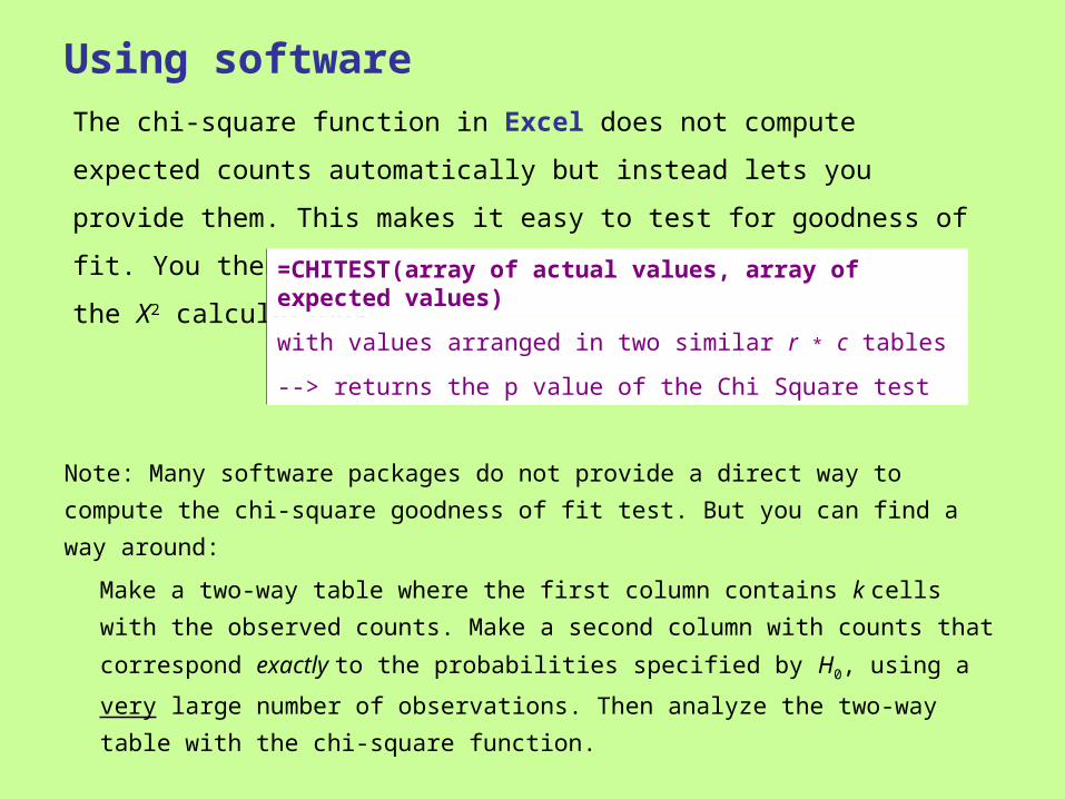
Using software

Note: Many software packages do not provide a direct way to compute the chi-

square goodness of fit test. But you can find a way around:

Make a two-way table where the first column contains k cells with the

observed counts. Make a second column with counts that correspond

exactly to the probabilities specified by H0, using a very large number of

observations. Then analyze the two-way table with the chi-square function.

The chi-square function in Excel does not compute expected counts

automatically but instead lets you provide them. This makes it easy to test for

goodness of fit. You then get the test’s p-value—but no details of the X2

calculations. =CHITEST(array of actual values, array of expected values)

with values arranged in two similar r * c tables

--> returns the p value of the Chi Square test

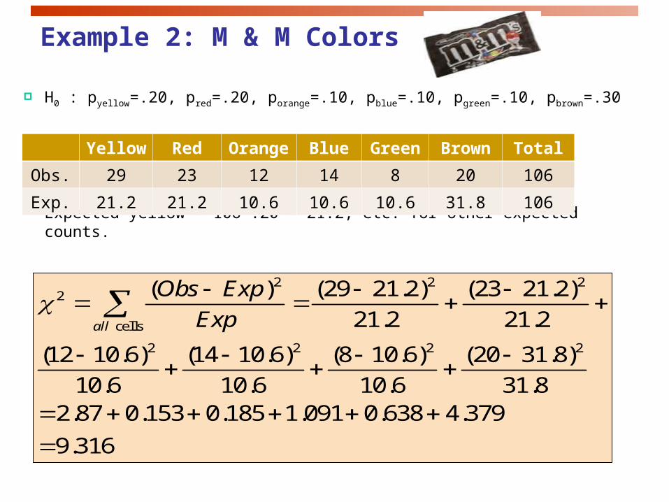
Example 2: M & M Colors

H0 : pyellow=.20, pred=.20, porange=.10, pblue=.10, pgreen=.10, pbrown=.30

Expected yellow = 106*.20 = 21.2, etc. for other expected counts.

Yellow Red Orange Blue Green Brown Total

Obs. 29 23 12 14 8 20 106

Exp. 21.2 21.2 10.6 10.6 10.6 31.8 106

2 2 22

cells

2 2 2 2

( ) (29 21.2) (23 21.2)

21.2 21.2

(12 10.6) (14 10.6) (8 10.6) (20 31.8)

10.6 10.6 10.6 31.82.87 0.153 0.185 1.091 0.638 4.379

9.316

all

Obs Exp

Exp

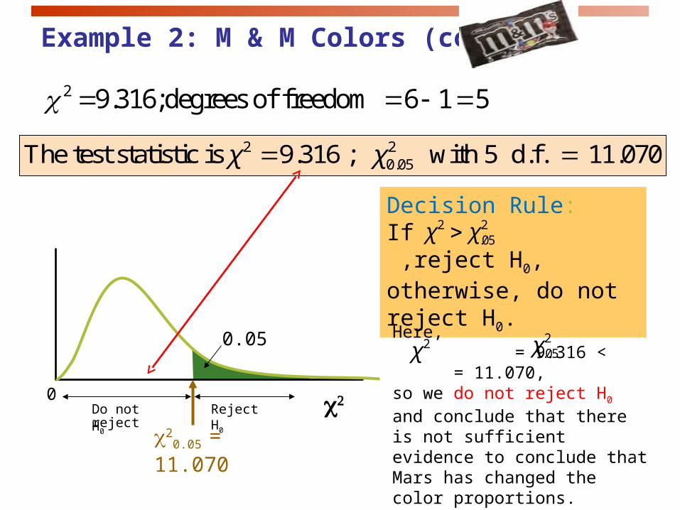
Example 2: M & M Colors (cont.)

2 9.316;degrees of freedom 6 1 5

2 20.05The test statistic is 9.316 ; with 5 d.f. 11.070χ χ

Decision Rule:If ,reject H0, otherwise, do not reject H0.

2 2.05χ χ

20.05 = 11.070

0

0.05

Reject H0Do not reject H0

Here, = 9.316 < = 11.070, so we do not reject H0 and conclude that there is not sufficient evidence to conclude that Mars has changed the color proportions.

2.05χ2χ

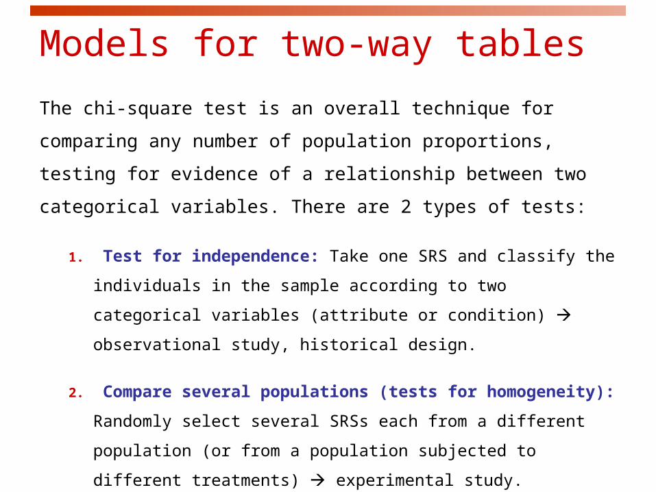
The chi-square test is an overall technique for comparing any number

of population proportions, testing for evidence of a relationship

between two categorical variables. There are 2 types of tests:

1. Test for independence: Take one SRS and classify the individuals in

the sample according to two categorical variables (attribute or condition)

observational study, historical design.

2. Compare several populations (tests for homogeneity): Randomly

select several SRSs each from a different population (or from a

population subjected to different treatments) experimental study.

Both models use the X2 test to test of the hypothesis of no relationship.

Models for two-way tables

Testing for independence

We have now a single sample from a single population. For each

individual in this SRS of size n we measure two categorical variables.

The results are then summarized in a two-way table.

The null hypothesis is that the row and column variables are

independent. The alternative hypothesis is that the row and column

variables are dependent.

Chi-square tests for independence

Expected cell frequencies:

Where:

row total = sum of all frequencies in the row

column total = sum of all frequencies in the column

n = overall sample size

22

cells

( )

all

Obs Exp

Exp

row total column total

nExp

H0: The two categorical variables are independent(i.e., there is no relationship between them)

H1: The two categorical variables are dependent(i.e., there is a relationship between them)

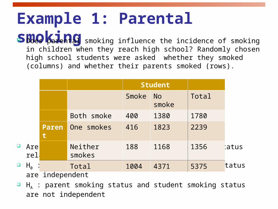
Example 1: Parental smoking Does parental smoking influence the incidence of smoking in

children when they reach high school? Randomly chosen high school students were asked whether they smoked (columns) and whether their parents smoked (rows).

Are parent smoking status and student smoking status related? H0 : parent smoking status and student smoking status are

independent HA : parent smoking status and student smoking status are not

independent

Student

Smoke No smoke Total

Both smoke 400 1380 1780

Parent One smokes 416 1823 2239

Neither smokes 188 1168 1356

Total 1004 4371 5375

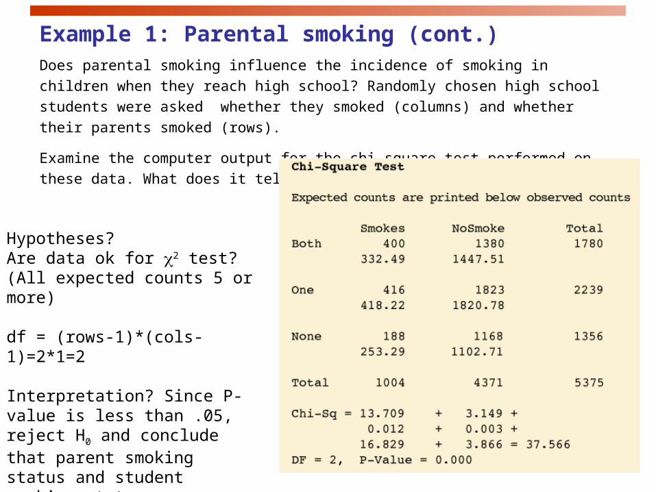
Example 1: Parental smoking (cont.)Does parental smoking influence the incidence of smoking in children when

they reach high school? Randomly chosen high school students were asked

whether they smoked (columns) and whether their parents smoked (rows).

Examine the computer output for the chi-square test performed on these data.

What does it tell you?

Hypotheses?Are data ok for 2 test? (All expected counts 5 or more)

df = (rows-1)*(cols-1)=2*1=2

Interpretation? Since P-value is less than .05, reject H0 and conclude that parent smoking status and student smoking status are related.

Example 2: meal plan selection

The meal plan selected by 200 students is shown below:

ClassStanding

Number of meals per week

Total20/week 10/week none

Fresh. 24 32 14 70

Soph. 22 26 12 60

Junior 10 14 6 30

Senior 14 16 10 40

Total 70 88 42 200

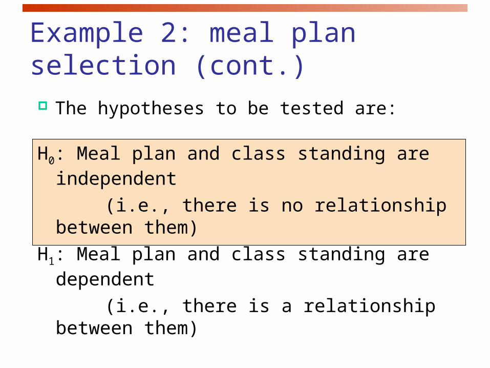
Example 2: meal plan selection (cont.) The hypotheses to be tested are:

H0: Meal plan and class standing are independent

(i.e., there is no relationship between them)

H1: Meal plan and class standing are dependent

(i.e., there is a relationship between them)

ClassStanding

Number of meals per week

Total

20/wk 10/wk none

Fresh. 24 32 14 70

Soph. 22 26 12 60

Junior 10 14 6 30

Senior 14 16 10 40

Total 70 88 42 200

ClassStanding

Number of meals per week

Total20/wk 10/wk none

Fresh. 24.5 30.8 14.7 70

Soph. 21.0 26.4 12.6 60

Junior 10.5 13.2 6.3 30

Senior 14.0 17.6 8.4 40

Total 70 88 42 200

Observed:

Expected cell frequencies if H0 is true:

row total column total

n30 70

10.5200

Exp

Example for one cell:

Example 2: meal plan selection (cont.) Expected Cell Frequencies

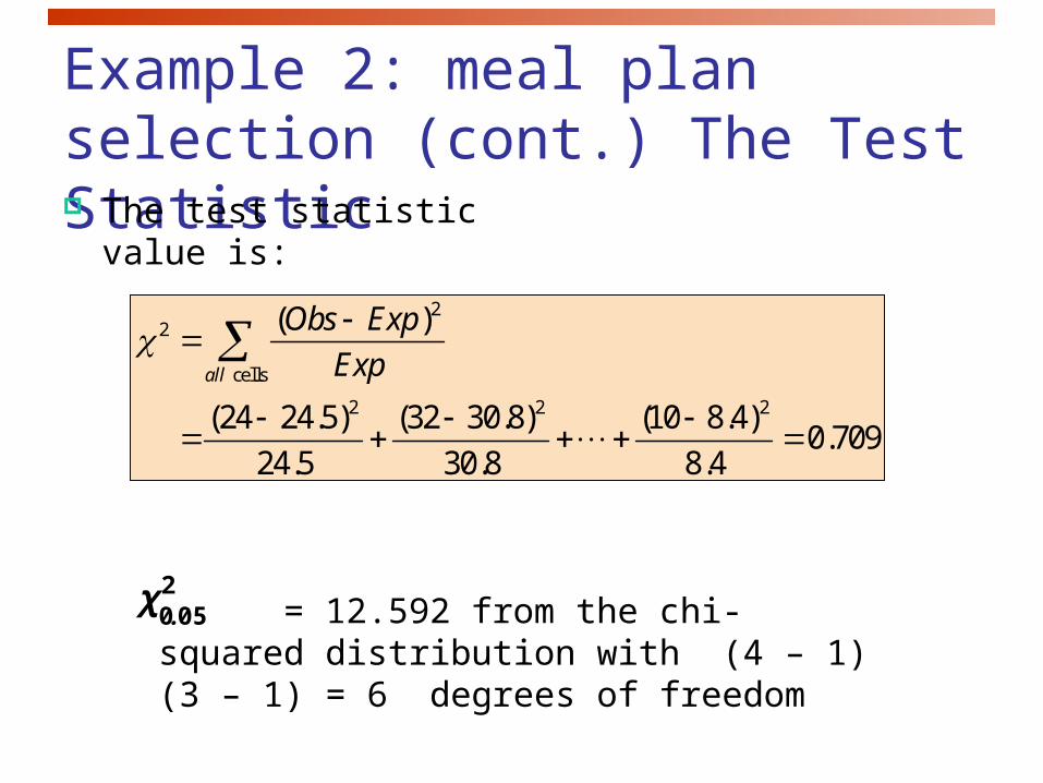
Example 2: meal plan selection (cont.) The Test Statistic The test statistic value is:

22

cells

2 2 2

( )

(24 24.5) (32 30.8) (10 8.4)0.709

24.5 30.8 8.4

all

Obs Exp

Exp

= 12.592 from the chi-squared distribution with (4 – 1)(3 – 1) = 6 degrees of freedom

2050.

χ

Example 2: meal plan selection (cont.) Decision and Interpretation

Decision Rule:If > 12.592, reject H0, otherwise, do not reject H0

2 20.05The test statistic is 0.709 ; with 6 d.f. 12.592

Here, = 0.709 < = 12.592, so do not reject H0 Conclusion: there is not sufficient evidence that meal plan and class standing are related.

20.05=12.592

0

0.05

Reject H0Do not reject H0

2

2 2050.

χ

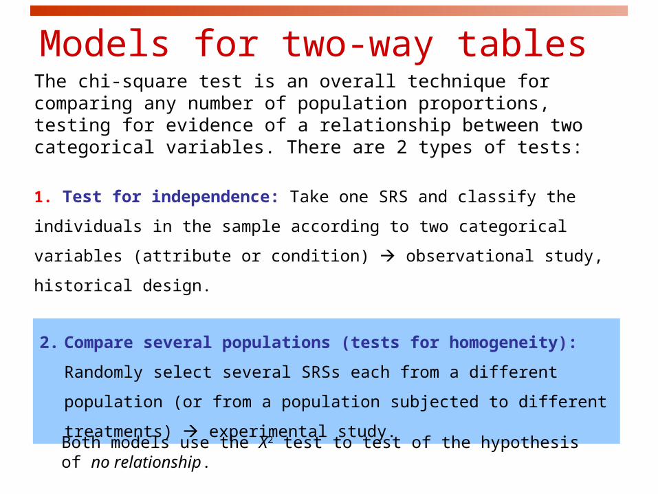
The chi-square test is an overall technique for comparing any number of population proportions, testing for evidence of a relationship between two categorical variables. There are 2 types of tests:

1. Test for independence: Take one SRS and classify the individuals in the

sample according to two categorical variables (attribute or condition)

observational study, historical design.

NEXT:

Models for two-way tables

2. Compare several populations (tests for homogeneity): Randomly

select several SRSs each from a different population (or from a population

subjected to different treatments) experimental study.

Both models use the X2 test to test of the hypothesis of no relationship.

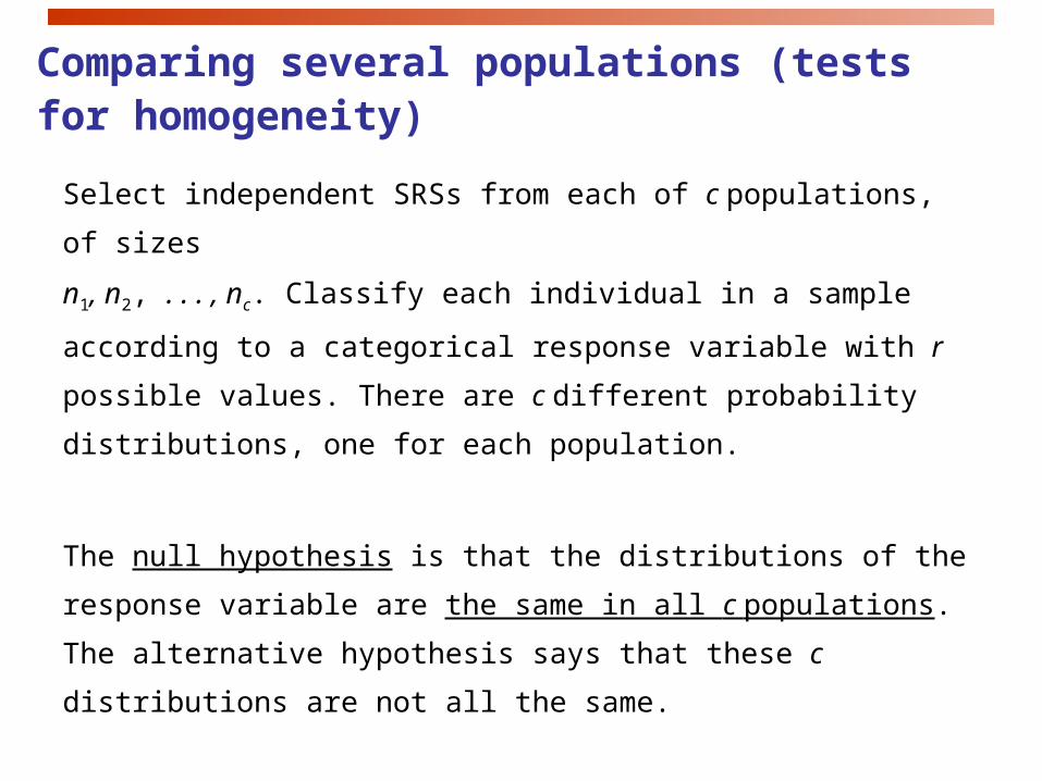
Comparing several populations (tests for homogeneity)

Select independent SRSs from each of c populations, of sizes

n1, n2, . . . , nc. Classify each individual in a sample according to a

categorical response variable with r possible values. There are c

different probability distributions, one for each population.

The null hypothesis is that the distributions of the response variable are

the same in all c populations. The alternative hypothesis says that

these c distributions are not all the same.

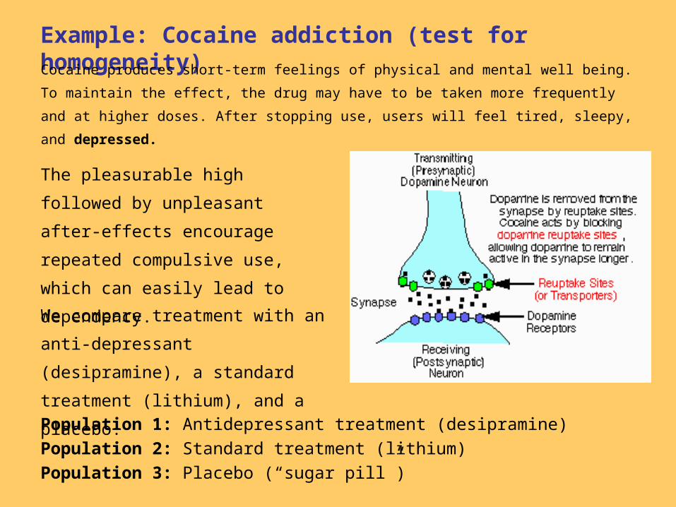
Example: Cocaine addiction (test for homogeneity)Cocaine produces short-term feelings of physical and mental well being. To

maintain the effect, the drug may have to be taken more frequently and at

higher doses. After stopping use, users will feel tired, sleepy, and depressed. 

The pleasurable high followed by

unpleasant after-effects encourage

repeated compulsive use, which can

easily lead to dependency. 

Population 1: Antidepressant treatment (desipramine)

Population 2: Standard treatment (lithium)

Population 3: Placebo (“sugar pill”)

We compare treatment with an anti-

depressant (desipramine), a standard

treatment (lithium), and a placebo.

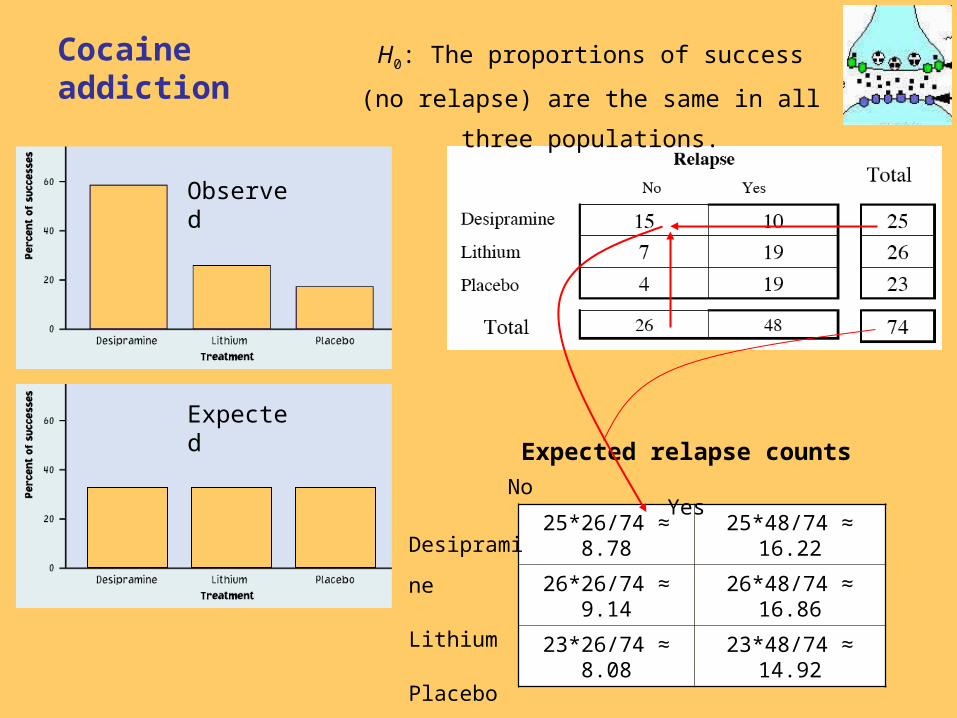
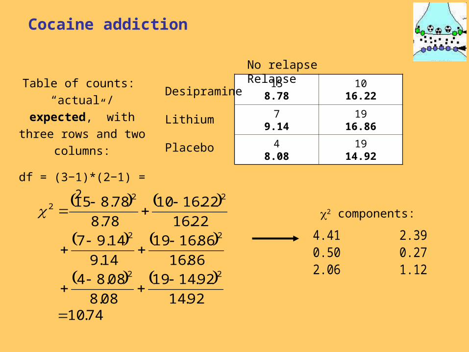
25*26/74 ≈ 8.78 25*48/74 ≈ 16.22

26*26/74 ≈ 9.14 26*48/74 ≈ 16.86

23*26/74 ≈ 8.08 23*48/74 ≈ 14.92

Desipramine

Lithium

Placebo

Expected relapse counts

No Yes

Expected

Observed

Cocaine addiction

H0: The proportions of success (no relapse)

are the same in all three populations.

Cocaine addiction

74.1092.14

92.1419

08.8

08.84

86.16

86.1619

14.9

14.97

22.16

22.1610

78.8

78.815

22

22

222

158.78

1016.22

79.14

1916.86

48.08

1914.92

Desipramine

Lithium

Placebo

No relapse Relapse

4.41 2.39 0.50 0.27 2.06 1.12

2 components:

Table of counts:

“actual / expected,” with

three rows and two

columns:

df = (3−1)*(2−1) = 2

Cocaine addiction: Table χ

X2 = 10.71 > 5.99; df = 2

reject the H0

H0: The proportions of success (no relapse)

are the same in all three populations.

ObservedThe proportions of success are not the same in

all three populations (Desipramine, Lithium,

Placebo).

Desipramine is a more successful treatment