Analysis of Critical Conditions in Electric Power Systems ...ijeei.org/docs-603739041542a94d20a02b.pdf · Analysis of Critical Conditions in Electric Power Systems by ... the line

International Journal on Electrical Engineering and Informatics - Volume 6, Number 3, September 2014

Analysis of Critical Conditions in Electric Power Systems by Feed Forward and Layer Recurrent Neural Networks

Ramaprasad Panda1, Pradyumna Kumar Sahoo2, Prasanta Kumar Satpathy3, and Subrata Paul4

1Silicon Institute of Technology (EEE Dept.), Bhubaneswar, Odisha, India

2ITER (PhD Scholar, EE Dept.), S’O’A University, Bhubaneswar, Odisha, India 3College of Engg. and Technology (EE Dept.), Bhubaneswar, Odisha, India

4Jadavpur University (EE Dept.), Kolkata, West Bengal, India [email protected]

Abstract: In this paper, critical conditions in electric power systems are monitored by applying various neural networks. In order to accomplish the stated goal, the authors tried several combinations of Feed Forward Neural Network and Layer Recurrent Neural Networks by imparting appropriate training schemes through supervised learning in order to formulate a comparative analysis on their performance. Once, training goes successful, the neural network learns how to deal with a set of newly presented data through validation and testing mechanism so as to evolve the best network structure and learning criteria. The proposed methodology has been tested on the standard IEEE 30-bus test system with the support of MATLAB based neural network toolbox. The results presented in this paper signify that the multi-layered feed forward neural network with Levenberg-Marquardt back propagation algorithm gives best training performance of all possible cases considered in this paper, thus validating the proposed methodology. Keywords: L-index, LCI, neural network, feed forward, back propagation Introduction

1. Introduction Critical conditions arising out of the risk of voltage instability [1], transmission line congestion management [2], and issues governing them are the major concern for any power system utility. There has been lots of research [3-9] indicating the risk imposed by critical operating conditions, which often lead to ultimate collapse of electric power systems. Basically, the critical condition analysis refers to identification of critical load buses through evaluation of L-index [10]. Most of the earlier studies based on conventional approach primarily depend on load flow simulation over a specific time period of observation and are faced with several limitations such as; complexity in modeling, unavailability of real time database, simulation of contingencies and more so. Hence, most of the present day research is inclined to get an edge over the same by supplementing the analysis with soft computing tools such as fuzzy logic and neural networks [11-16]. Being partially motivated by this, the authors of this paper have tried to implement neural network tools for identification of critical conditions in electric power system through a comparative study and performance analysis of the proposed network with the basic objective of evolving an optimal network structure and learning criteria. Further, it is learnt that a thoroughly trained neural network becomes capable of learning from these events so that the trained network could be exposed to any set of input data in a future time for necessary validation and testing purpose [17]. Hence, the authors highly feel that application of neural network principles to power systems could possibly bring some improvements resulting in faster analysis with lesser complexity by way of avoiding repeat execution of the conventional load flow program. In this proposed work, the authors have tried to formulate a permanent database of events, corresponding information on critical ranking of bus bars covering all such possible events and situations that might come on the way of power system operation. The database so obtained

Received: April 15th, 2014. Accepted: August 15th, 2014

447

could serve the role of input data and target data so as to be presented before the neural network for imparting a thorough training through successive supervisory learning mechanism. Thus, the burden of repeat execution of the load flow program for monitoring the critical conditions in a dynamic time frame could be relieved significantly. Secondly, in order to improvise the performance of the proposed neural network, the authors have tried a comparative analysis considering two important types of neural network schemes such as Feed Forward Neural Network (FFNN) and Layer Recurrent Neural Network (LRNN) for formulation of an optimal neural network structure for this purpose. In consideration of these facts, the paper is organized as follows. Section 2 highlights the methodology behind formation of the L-index that would serve as the indicator for grading the system buses in order of their criticality for a specified event, be it the normal base case operating condition or any contingent condition otherwise. Section 3 presents the background of neural network structure and its applicability to this problem. In this section the authors have considered multiple layered feed forward neural networks supplemented with various types of back propagation algorithms and layer recurrent neural networks for a comparative performance analysis. In addition to this, various combinations of hidden layers and placement of neurons in those layers have been considered too. In Section 4, a detailed case study is presented through implementation of the proposed methodology in the standard IEEE 30-bus test system. The simulation results justify that the algorithm works well in all situations, as evident from the convergence during training, thus offering minimal error goal to reach the specific target. From the comparative performance analysis of section 4 it is inferred that the proposed feed forward neural network along with the Levenberg-Marquardt back propagation algorithm performed the best in terms of iterations required and speed of convergence. 2. Evaluation of Indices for Critical Conditions In general, the performance of electrical power utilities remains almost stable during base case loading scenario. However, in a complex dynamic system like this, the operating conditions remain hardly static at the base loading. Therefore, it becomes mandatory to monitor the system’s performance with contingent conditions so as to assess critical issues like margin to voltage instability and line congestion level during such worse situations. In this paper, the contingency related to load growth has been simulated through simultaneous increase in the load demand at the load buses with additional step loading above the base load. This is accomplished by use of a multiplying factor (λ). Assuming that the complex load demand at bus-i during base case is denoted by ‘Si,base’, the load increasing scenario for any future time ‘Si’ is expressed as a function of ‘Si,base’ as indicated in Equation (1):

1 , (1)

It may also be noted here that a zero value for the load multiplying factor refers to base case loading condition and non-zero positive values greater than zero refers to higher loading beyond the base case. The critical condition described by margin to voltage instability is presented through L-index, which is usually derived from the load flow solution by making use of the impedance matrix of the system as the study parameter. The L-index offers a minimum value of ‘0’ and maximum value of ‘1’ indicating stable and unstable condition of the power system, respectively, which gives a quantitative measure for the estimation of the distance of the actual state of the system with respect to the limiting state of voltage stability and hence serves as a good indicator describing the stability of the complete system. In the beginning, a complex gain matrix of the power system is obtained by using the self admittance matrix of individual buses and the mutual admittance matrix between the generator buses and load buses. Then, for a system having ‘G’ number of generators, the L-Index (Lj) for the jth load bus could be defined as an absolute function of gain matrix (Fji) and the ratio of generator bus voltages (Vi) to that of the load bus voltages (Vj), as indicated in Equation (2):

Ramaprasad Panda, et al.

448

1 ∑ (2)

Also, L-index could be defined as a function of the complex power, admittance matrix and voltage magnitude, as indicated in Equation (3):

(3)

Another critical condition in power system operation described by transmission line congestion has also been used in this work. The congestion level designated through an index called line congestion index (LCI) is based on the most fundamental principles of electrical power system studies, such as, characteristics of transmission lines, their performance and load flow studies. In a particular power system case, the load current is governed mostly by the impedance of the load connected at the receiving end of the line. While, the load impedance matches exactly with the characteristic impedance/surge impedance of the line, the line gets eventually terminated by its own characteristic impedance resulting in an infinite line and the then power supplied to the load through the line is called surge impedance loading (SIL) of the line, as indicated in Equation (4):

| | (4)

A comparison between the actual value of real power being transmitted in a particular line (Pl) with its own surge impedance loading (SIL) could be established as a measure or an indicator of the congestion level in that particular line. Thus, the LCI is treated as the ratio of the two powers, as given in Equation (5):

(5)

It is noteworthy to be mentioned here that the lines having higher values of LCI are to be treated as more congested in terms of their power handling capacity and safe thermal limit. While evaluating the critical indices for a particular configuration and an underlying situation of any system, the focus is primarily made so as to maintain the voltage at the candidate load buses within specified limits as referred by the grid code. 3. Problem Formulation based on Neural Network Analysis The literature indicates successful application of neural networks in solving complex real world problems with ease and has been widely accepted by researchers in the area of electrical power systems [18-24]. Though it is justified in most of the reported findings that neural networks are performing well in the context of analyzing complex mappings accurately and rapidly, yet finding an optimal network and learning criterion to suit a particular problem remained the major concern. These facts motivated the authors to implement neural network principles for obtaining approximate, faster results in identifying critical conditions while developing a comparison on the performance of various neural network structures. A generalized structure of the neural network comprises of an input stage, an output stage and few hidden layers. The hidden layers contain neuron like elements having interconnectivity, which by and large determine the functioning of the network. These simulated neurons have been designed to behave in more or less similar way in response to

Analysis of Critical Conditions in Electric Power Systems by Feed

449

input signals, as those of the biological neurons in the brain cells of living beings. Each connection is associated with an index called weight parameter (w) that transforms the input (p) in accordance with the weighting index in order to present a specific output (a). Such networks also have the ability to synthesize the internal structure of the neurons through assignment and adjustment of weights, based on the exposure, experience and learning skill they acquire through training. A single line diagram of a simple neuron model is shown in Figure 1, so as to illustrate the functional mechanism of handling the weights while transforming a given input into a corresponding output in absence of any bias (b). A similar presentation of the single line diagram of a simple neuron model illustrating the input-output relationship in presence of both weights and bias parameters is shown in Figure 2. The bias is much like the weight, except the fact that bias is always assigned a constant unit value (b=1). The mathematical form of the output for the network architectures shown in Figures 1 and 2, are given respectively in Equations (6) and (7):

(6)

(7)

Though, there is no restriction in making a suitable selection of the transfer function (f), it could preferably be any of the mathematical functions described by hard-limiting, linear, logarithmic, sigmoid functions or any combination of these ones such as log-sigmoid or tan-sigmoid. In this work the authors have used tan-sigmoid transfer function for the hidden layers and linear transfer function for the output layers as shown in Figure 3. The process by which the neural network learns is called training process. The training objective may be set to obtain various goals such as approximation of functions and pattern association or pattern classification of data sets. In order to start with the training, it is desirable that the weights and bias associated with the neurons be properly initialized. The learning rules for the training are of two types such as supervised learning and unsupervised learning. In case of supervised learning, the neural network is trained with the help of a training set comprising of actual inputs and their corresponding correct outputs (treated as the target). However, in unsupervised learning, the neural network is trained in response to network inputs only as the target outputs are not available. In this paper, supervised learning has been followed supported with back propagation algorithm. The neural network structure for FFNN and LRNN considering two hidden layers and an output layer are shown in figure 4 and figure 5, respectively. As evident from the working principles of machine learning [25], two types of datasets are essential for imparting supervised training to any neural network such as input data and target data. Since the objective of this work is primarily aimed at evaluating the performance of neural networks through identification of critical conditions, the authors feel that the information on critical grading of buses (L-index) would best serve the input dataset. Any other parameter of the system that more or less signifies the critical operation of the system could be considered. Hence, a corresponding set of LCI has been considered to form the target data. The weights and bias parameters need to be adjusted during training process in order to minimize the network performance function until the net output falls within closely tolerable/ acceptable proximity to the target set by the operator. It could take few iterations/epochs during each cycle of training before the neural network gets properly trained so as to rationalize newer inputs through mapping by utilizing the experience acquired during earlier training. The process of exposing the trained neural network to a predefined input dataset is termed as validation and testing, which is essential for validating the correctness of the trained neural network. The ability of neural networks to adapt to particular or random inputs could be very well assessed from graphical plots such as performance plots, error surface (ES) plots, and bar graphs showing the resulting percentage classification of various data sets such as detection


450

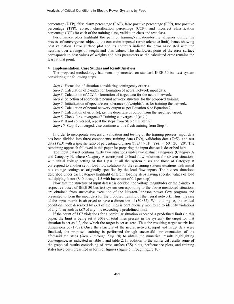
percentage (DTP), false alarm percentage (FAP), false positive percentage (FPP), true positive percentage (TPP), correct classification percentage (CCP), and incorrect classification percentage (ICP) for each of the training class, validation class and test class. Performance plots highlight the path of training/validation/testing schemes during the process of convergence subject to the constraint imposed (error tolerance limit), hence showing best validation. Error surface plot and its contours indicate the error associated with the neurons over a range of weight and bias values. The shallowest point of the error surface corresponds to best values of weights and bias parameters as the calculated error remains the least at that point. 4. Implementation, Case Studies and Result Analysis The proposed methodology has been implemented on standard IEEE 30-bus test system considering the following steps.

Step 1: Formation of situation considering contingency criteria. Step 2: Calculation of L-index for formation of neural network input data. Step 3: Calculation of LCI for formation of target data for the neural network. Step 4: Selection of appropriate neural network structure for the proposed training. Step 5: Initialization of epochs/error tolerance (ε)/weights/bias for training the network. Step 6: Calculation of neural network output as per Equation 6 or Equation 7. Step 7: Calculation of error (e), i.e. the departure of output from the specified target. Step 8: Check for convergence? Training converges, if (e ≤ ε). Step 9: If not converged, repeat the steps from Step 5 till Step 8. Step 10: Stop if converged, else continue with a fresh training from Step 4.

In order to incorporate successful validation and testing of the training process, input data has been divided into three components; training data (TrD), validation data (VaD), and test data (TeD) with a specific ratio of percentage division ( 60 20 20). The remaining approach followed in this paper for preparing the input dataset is described here. The input dataset contains thirty two situations under two distinct categories (Category A and Category B, where Category A correspond to load flow solutions for sixteen situations with initial voltage setting of flat 1 p.u. at all the system buses and those of Category B correspond to another set of load flow solutions for the remaining sixteen situations with initial bus voltage settings as originally specified by the load flow inputs. The sixteen situations described under each category highlight different loading steps having specific values of load multiplying factor (λ=0 through 1.5 with increment of 0.1 per step). Now that the structure of input dataset is decided, the voltage magnitudes or the L-index at respective buses of IEEE 30-bus test system corresponding to the above mentioned situations are obtained from successive execution of the Newton-Raphson power flow program and presented to form the input data for the proposed training of the neural network. Thus, the size of the input matrix is observed to have a dimension of (30×32). While doing so, the critical condition index described by LCI of the lines is continuously monitored to identify violations of any form such as LCI of any line exceeding a predefined limit. If the count of LCI violations for a particular situation exceeded a predefined limit (in this paper, the limit is being set at 30% of total lines present in the system), the target for that situation is set as ‘1’, else which the target is set as zero. Thus the resulting target matrix has dimensions of (1×32). Once the structure of the neural network, input and target data were finalized, the proposed training is performed through successful implementation of the aforesaid ten steps (Step 1 through Step 10) to obtain the numerical results highlighting convergence, as indicated in table 1 and table 2. In addition to the numerical results some of the graphical results comprising of error surface (ES) plots, performance plots, and training states have been presented in form of figures (figure 6 through figure 10).


451

Table 1. Neural Network (FFNN) Performance Analysis Parameters Assigned for the Neural Network Training Results (convergence) Feed Forward

Neural Network (FFNN)

with Levenberg-Marquardt

Backpropagation

Number of hidden layers

Neurons in each

hidden layer

Number of training cycles

performed

Number of epochs used

during the last cycle

Time taken for training

convergence in seconds

Maximum Epochs/cycle=100 (Error tolerance

limit=0.001)

1

1 670 8 290 2 1041 6 455 3 35 5 20 4 511 10 231 5 1038 7 509

2

1* 41 11 23 2 107 8 50 3 387 7 173 4 790 11 391 5 685 6 351

3

1 86 17 46 2 52 5 28 3 502 11 257 4 313 7 163 5 66 4 38

4

1 806 6 422 2 80 9 40 3 213 11 109 4 210 7 113 5 693 8 406

5

1 320 4 162 2 7 4 7 3 229 4 135 4 30 5 21 5 235 6 155


limit=0.001)

1 2 1041 6 455

3 35 5 20

2 1* 608 8 270 2 107 8 50

3 2 52 5 28 4 2 80 9 40 5 2 7 4 7

During the trial sessions of training, it has been observed that arbitrary selection of parameters (error tolerance limit, limiting number of epochs assigned during training cycles, number of hidden layers and number of neurons in the hidden layers) bear lots of significance towards successful convergence. Further, it is also observed that the training suffered from limitations leading to either non-convergence or delayed convergence with assignments of higher epoch limit and lower error tolerance limit. However, convincingly faster convergence is observed with error tolerance setting of 0.001, and epoch setting of 100 epochs per training cycle. Thus, the final training has been dealt in this paper with these golden settings and the convergence results for two types of neural networks with different combinations of hidden layers and neuron distribution have been presented in this paper for drawing up a comparative performance analysis.


452

Table 2. Neural Network (LRNN) Performance Analysis Parameters Assigned for the Neural Network Training Results (convergence)

Layer Recurrent Neural Network (LRNN)

with Levenberg-Marquardt

Backpropagation

Number of hidden layers

Neurons in each hidden

layer

Number of training cycles

performed

Number of epochs used during the last cycle

Time taken for training convergence in seconds


limit=0.001)

1

1 202 4 129 2 229 5 159 3 510 4 330 4 55 6 40 5 436 8 334

2

1 469 7 489 2 27 7 30 3 28 9 31 4 251 9 278 5 852 8 1042

3

1 105 5 186 2 58 10 122 3 23 8 40 4 45 6 82 5 122 6 237

4

1 113 12 296 2 266 21 767 3 90 7 230 4 247 15 729 5 607 7 1812

5

1 362 8 1482 2# 9 11 42 3$ 280 6 1281 4 188 32 855 5 928 4 5788


limit=0.001)

1 4 55 6 40 3 510 4 330

2 2 27 7 30 3 28 9 31

3 3 23 8 40 4 3 90 7 230

5 2# 263 3 992 3$ 150 10 579

In order to justify the comparative analysis for each neural network structure under study (i.e. FFNN and LRNN structures), the authors have presented the convergence results for few cases having same error tolerance setting (0.001), but a different epoch setting of 10 epochs per training cycle. Only those deserving cases having lowest order of convergence time under epoch setting of 100 epochs per training cycle have been reflected in this segment in order to verify their consistency with epoch setting of 10 epochs per training cycle. From the numerical results of Table 1 it observed that almost all cases (except one case*) had same results of convergence, consistently for both the epoch settings. The numerical results of Table 2 also indicated consistency in convergence for almost all cases (except two cases#,$) for both the epoch settings. Although, it could not be possible to generalize the numerical results of Table 1 with those of Table 2, yet one thing that is strikingly observed from these results that both the neural networks (FFNN and LRNN) indicated good convergence for all possible combinations of hidden layer and neuron variations, thereby justifying their application to electric power systems for monitoring the critical conditions with ease. However, a measure of convergence time as low as 7-seconds figuring in Table 1 (hopefully the least of all values in both Table 1 and Table 2) with five hidden layers and two neurons per layer could establish the superiority of FFNN over LRNN.


453

The graphical results for the particular case of Table 1 having lowest convergence time are shown in Figure 6 through Figure 10. While, Figure 6 shows the performance plot with best validation performance at epoch-4, the plot in Figure 7 indicates the error surface and error contours. In this plot the white circle highlights the least error during training convergence. Figure 8 indicates the percentage classification of various rates during training, with TPP and CCP values of 80% and 100% respectively, hence indicating perfection in training. Figure 9 indicates the percentage classification of various rates during validation, with TPP and CCP values of 100% each, thus indicating perfect validation. Figure 10 indicates the percentage classification of various rates during testing, with TPP and CCP values of 84% and 100% respectively, thereby indicating perfection in testing. It is observed from these plots that the criteria of training perfection are very well met by the proposed algorithm and methodology and the proposed feed forward neural network along with the Levenberg-Marquardt back propagation may be considered as the most suitable neural network for this study. 5. Conclusion The basic objective of finding a trained neural network in order to monitor critical conditions in power system operation has been met quite successfully in this paper. In the beginning, an exhaustive set of load flow results are obtained (once for all) for formation of input and target data for each situation. These situations cover base case condition, steady and gradual loading around the network and contingencies as well. In this paper, all these aspects have been considered with proper coordination of issues relating to preparation of input and target data sets, selection of neural network structure including number of hidden layers and neurons in the layers, and assignment of weights/bias to the neurons so as to impart successful training. The major advantage of this application would be to get rid of the complexity involved in finding similar results from the load flow calculations, which are time consuming and tedious. The utilities are expected to benefit a lot from this approach without sacrificing much on accuracy. This objective has been worked out with the proposed methodology in support of MATLAB based Matpower computing platform and the results are validated through the case studies conducted on standard IEEE test systems. The results of the case study conducted on a standard IEEE 30-bus test system justifies the validity of the findings which also satisfy all the required conditions for a perfectly trained neural network. 6. References [1] Concordia C. Voltage Instability. Electrical Power and Energy Systems 1991; 13(1):14-

20. [2] Kumar A, Srivastava SC, Singh SN. Congestion Management in Competitive Power

Market: A Bibliographical Survey. Electric Power Systems Research 2005; 76:153-164. [3] Yorino N, Sasaki H, Masuda Y, Tamura Y, Kitagawa M, and Oshimo A. An investigation

of Voltage Instability Problems. IEEE Trans on Power Systems 1992; 7(2):600-611. [4] Ajjarapu V, and Lee B. Bibliography on Voltage Stability. IEEE Trans on Power Systems

1998; 13:115-125. [5] IEEE Task Force. Proposed Terms and Definitions for Power System Stability. IEEE

Trans on Power Apparatus and Systems 1982; 101:1894-1898. [6] Miller NW, and Price WW. Planning and Operations Benefits of High Fidelity Voltage

Collapse Simulations. Electrical Power and Energy Systems 1993; 15(4):245-250. [7] Deuse J, and Stubbe M. Dynamic Simulation of Voltage Collapse. IEEE Trans on Power

Systems 1993; 8(3):894-904. [8] Tamura Y, Mori H, and Iwamoto S. Relationship between Voltage Instability and

Multiple Load Flow Solutions in Electric Power Systems. IEEE Trans on Power Apparatus and Systems 1983; 102:1115-1123.

[9] Cutsem TV. A Method to Compute Reactive Power Margin to Voltage Collapse. IEEE Trans on Power Systems 1991; 6(2):145-156.


454

[10] Kessel P, and Glavitsch H. Estimating the Voltage Stability of a Power System. IEEE Trans on Power Delivery 1986; 1:346-354.

[11] Hawary ME. Electric Power Applications of Fuzzy Systems. IEEE Press, 1998. [12] Zadeh LA. Fuzzy Sets as a basis for a theory of Possibility. Fuzzy Sets and Systems 1978;

1:3-28. [13] Zimmerman HJ. Fuzzy Set Theory and its Application. Kluwer Academic Press, 1994. [14] Bahamanyar AR, and Karami A. Power System Voltage Stability Monitoring using

Artificial Neural Networks with a Reduced set of Inputs. Electrical Power and Energy Systems 2014; 58:246-256.

[15] Zhou DQ, Annakkage UD, and Rajapakse AD. Online Monitoring of Voltage Stability Margin Using an Artificial Neural Network. IEEE Trans on Power Systems 2010; 25(3):1566-1574.

[16] Keib AAE, and Ma X. Application of Artificial Neural Networks in Voltage Stability Assessment. IEEE Trans on Power Systems 1995; 10(4):1890-1896.

[17] Mirzaei M, Kadir MZA, Hizam H, and Moazami E. Comparative Analysis of Probabilistic Neural Network, Radial Basis Function, and Feed-forward Neural Network for Fault Classification in Power Distribution Systems. Electric Power Components and Systems 2011; 39:1858-1871.

[18] Kalra PK, Srivastava A, and Chaturvedi DK. Artificial neural nets applications to power systems operation and control. Electric Power Systems Research 1992; 25:83-90.

[19] Dillon TS. Artificial neural nets applications to power systems and their relationships to symbolic methods. Electrical Power and Energy Systems 1991; 13:66-72.

[20] Sharkawi El, Marks MA, and Weerasoritya RJ. Neural Networks and their Application to Power Engineering. Control Dynamic System, Advances in theory and Applications 1991; 41(1/4).

[21] Ranaweera DK. Comparison of neural network models for fault diagnosis of power systems. Electric Power Systems Research 1994; 29(2):99-104.

[22] Hagan MT, and Menhaj M. Training feed-forward networks with the Marquardt algorithm. IEEE Transactions on Neural Networks 1994; 5(6):989-993.

[23] Ilamathi B, Selladurai VG, and Balamurugan K. ANN-SQP Approach for NOx emission reduction in Coal Fired Boilers. Emerging Electric Power Systems 2012; 13(3):1-14.

[24] Xue L, Jia C, and Dajun D. Comparison of Levenberg-Marquardt method and Path Following interior point method for the solution of optimal power flow problem. Emerging Electric Power Systems 2012; 13(3):15-35.

[25] Mitchell T. Machine Learning. Boston, MA, WCB/McGraw-Hill 1997.

Figure 1. Neuron architecture with weights only

Figure 2. Neuron architecture with weights and bias


455

Figure 3. Transfer functions for hidden layer (tansig) and output layer (linear)

Figure 4. Structure of Feed Forward Neural Network (FFNN) with two hidden layers

Figure 5. Structure of Layer Recurrent Neural Network (LRNN) with two hidden layers

Figure 6. Performance plot of FFNN for optimum convergence

0 0.5 1 1.5 2 2.5 3 3.5 410-12

10-10

10-8

10-6

10-4

10-2

100Best Validation Performance is 4.697e-012 at epoch 4

Mea

n S

quar

ed E

rror

(mse

)

4 Epochs

TrainValidationTestBestGoal


456

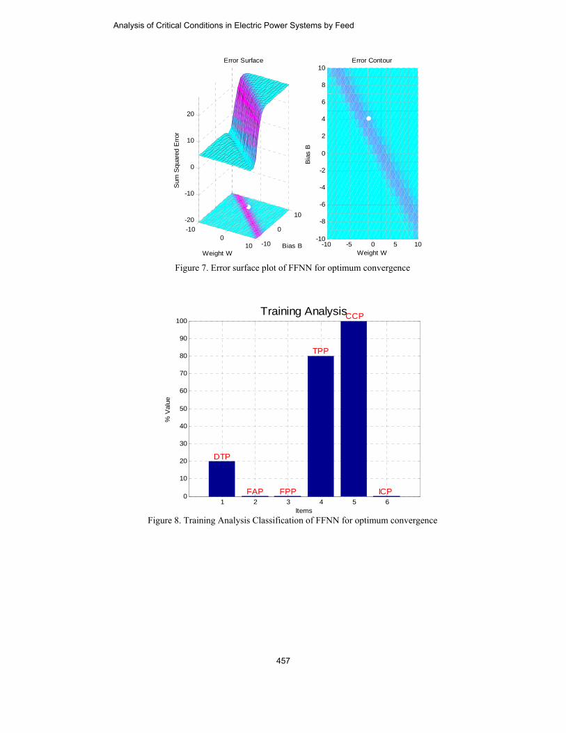
Figure 7. Error surface plot of FFNN for optimum convergence

Figure 8. Training Analysis Classification of FFNN for optimum convergence

-100

10 -10

0

10-20

-10

0

10

20

Bias B

Error Surface

Weight W

Sum

Squ

ared

Erro

r

-10 -5 0 5 10-10

-8

-6

-4

-2

0

2

4

6

8

10

Weight W

Bia

s B

Error Contour

1 2 3 4 5 60

10

20

30

40

50

60

70

80

90

100Training Analysis

Items

% V

alue

DTP

FAP FPP

TPP

CCP

ICP


457

Figure 9. Validation Analysis Classification of FFNN for optimum convergence

Figure 10. Test Analysis Classification of FFNN for optimum convergence

1 2 3 4 5 60

10

20

30

40

50

60

70

80

90

100Validation Analysis

Items

% V

alue

DTP FAP FPP

TPP CCP

ICP

1 2 3 4 5 60

10

20

30

40

50

60

70

80

90

100Test Analysis

Items

% V

alue

DTP

FAP FPP

TPP

CCP

ICP


458

RamEnginSubseASICAllahSysteas AsSilico

PradEnginthe yEnginUnivhis Ph

PrasEnginSubsfromdegre(IndiEnginOdis

SubrElect1982SysteProfeUniv

maprasad Panneering from equently, he a

C Design fromhabad (India) dems at Jadavpussociate Profeson Institute of T

dyumna Kumaneering as an

year 2003. Conneering from ersity, Bhubanh.D. in S’O’A

santa Kumar Sneering from

sequently, he m Indian Institu

ee in Power Sia) during 20neering in Cha, India.

rata Paul obtatrical Engineer

2 respectively. ems from Jadaessor with thversity, kolkata

nda obtained Bangalore

acquired his Mm Motilal Neduring 2004 anur University, ssor, Electrical Technology, B

ar Sahoo obtaiAssociate Memnsequently he Institute of T

neswar, OdishaUniversity, Bh

Satpathy obtaiSambalpur Unacquired M.T

ute of TechnolSystems from I03. Currently

College of En

ained Bachelorring from Jadav

Subsequentlyavpur Univers

he Departmenta (West Bengal

his under graUniversity, K

M.Tech. Degreeheru Nationand is pursuingKoklkata (Indand Electronic

Bhubaneswar, O

ined his under mber of Instituobtained his Mechnical Educ

a in the year 20hubaneswar, O

ined his under niversity, Odisech. degree inlogy, Delhi (InIndian Institute

he is workingineering &

r in Electrical vpur Universit

y, he acquired sity, Koklkata t of Electrical), India.

aduate degreeKarnataka, Indee in Power Eal Institute ofg his Ph.D. dedia). Currently cs EngineeringOdisha, India.

graduate degreution of EnginM.Tech. degrecation and Res009. Currently

Odisha

graduate degresha, India in tn Electrical Pndia) during 19e of Technoloing as ProfesTechnology,

Engineering aty, India in the

his Ph.D. deg(India) in 200

al Engineering

e in Electricaldia in 1990

Electronics andf Technology,

egree in Powerhe is working

g department in

ee in Electricalneers (India) inee in Electricalsearch, S’O’Ahe is pursuing

ee in Electricalthe year 1989

Power Systems996 and Ph.Dgy, Kharagpursor, ElectricalBhubaneswar,

and Masters inyear 1980 and

gree in Power06. Dr Paul isg at Jadavpur

l .

d , r g n

l n l

A g

l . s . r l ,

n d r s r


459

Documents

Analysis of Critical Conditions in Electric Power Systems ...ijeei.org/docs-603739041542a94d20a02b.pdf · Analysis of Critical Conditions in Electric Power Systems by ... the line