AALTO UNIVERSITY School of Electrical Engineering Department of Communications and Networking

Analysis of Energy Efficiency in IEEE 802.11ah Yue Zhao

Master's Thesis submitted in partial fulfillment of the degree of Master of Science in Technology Espoo, 19th May 2015 Supervisor: Prof. Olav Tirkkonen Instructor: M.Sc. Osman N. C. Yilmaz

i

AALTO UNIVERSITY

Abstract

Author:

Name off the Thesis:

Zhao Yue

Analysis of Energy Efficiency in IEEE 802.11ah

Date: 19 May 2015 Number of pages: 11 + 50 = 61

Department:

Degree Program:

Department of Communications and Networking

Degree Program in Communications Engineering

Supervisor:

Instructor:

Prof. Olav Tirkkonen

M.Sc. Osman N. C. Yilmaz

Recently, machine to machine (M2M) communication has been considerably evolved and occupied a large proportion of the wireless markets. The distinct feature of M2M applications brings new challenges to the design of the wireless systems. In order to increase the competence for M2M markets, several enhancements have been proposed accordingly in different wireless technologies. The thesis introduces these M2M enhancements with a focus on the Wi-Fi solution - 802.11ah technology.

802.11ah is a new amendment of Wi-Fi technology for M2M applications. In 802.11ah, a new mechanism named TIM segmentation has been introduced to provide scalable operation for a large number of devices as well as reduce the energy consumption. The scope of the thesis is to evaluate the energy efficiency of TIM segmentation in uplink traffic assuming Poisson process. To thoughtfully understand the principle of this mechanism, the fundamental MAC layer functions in Wi-Fi technologies have also been introduced. In addition, the thesis also proposed an energy-saving solution called additional sleeping (AS) cycles.

The performance evaluation is based on a Matlab system-level simulator. The simulations are carried out for various TIM segmentation deployments for a selected M2M use case, the agriculture scenario. The results show that the TIM segmentation can deteriorate the performance for uplink transmission. This is because that in sporadic traffic, restricting the uplink access causes the increase in packet buffering and these packets leads to simultaneous transmission. This can be a serious issue especially for the network with a large number of devices. The random backoff procedure in Wi-Fi cannot efficiently solve this collision problem. In addition, results shows that the AS cycles can reduce the energy consumption in busy-channel sensing and also decrease the collision probability by adding extra randomness.

Key words: IEEE 802.11ah, Energy Efficiency, M2M, IoTs

ii

Preface

First and foremost I would like to deeply thank my advisors, Prof. Olav Tirkkonen and

M.Sc. Osman N. C. Yilmaz for their excellent guidance and valuable comments on

simulations and background studies.

I also wish to thank my colleagues from Ericsson Research Finland for their support and

encouragement throughout the thesis work.

Finally, I would like to express my deepest gratitude and respect to my family, especially

my wife to whom I owe everything I have achieved, for her love and invaluable support.

Espoo, 19 May 2015

Yue Zhao

iii

Table of Contents

Abstract .............................................................................................................................. i

Preface ............................................................................................................................... ii

Table of Contents ............................................................................................................. iii

List of Abbreviations .......................................................................................................... v

1 Introduction .................................................................................................................... 1

2 M2M Enhancement in wireless technologies ................................................................ 4

2.1 LTE Enhancement for M2M ..................................................................................... 4

2.1.1 Enhancement for low cost device ..................................................................... 4

2.1.1.1 Device Category 0 in Release-12 ................................................................ 4

2.1.1.2 Device Category low cost in Release 13 ..................................................... 5

2.1.2 Energy Saving for Years of Battery Life ............................................................. 5

2.1.2.1 Extended Discontinuous Reception ........................................................... 5

2.1.2.2 Device Power Saving Mode ........................................................................ 6

2.1.3 Enhancement for deep coverage ...................................................................... 7

2.1.4 Scalability Improvement ................................................................................... 7

2.2 M2M Enhancements in Short Range Radio Technologies ....................................... 8

2.2.1 Wi-Fi .................................................................................................................. 8

2.2.2 Bluetooth .......................................................................................................... 8

3 Fundamentals of Wi-Fi Technology .............................................................................. 10

3.1 Introduction to Wi-Fi ............................................................................................. 10

3.2 Connection Management ...................................................................................... 11

3.3 PHY layer ................................................................................................................ 12

3.4 MAC layer ............................................................................................................... 13

3.4.1 Channel Access ................................................................................................ 13

3.4.1.1 Distributed Coordination Function .......................................................... 14

3.4.1.2 Enhanced Distributed Channel Access ..................................................... 16

3.4.2 Request to Send/Clear to Send Mechanism ................................................... 17

3.4.3 Virtual Carrier Sense ....................................................................................... 18

3.5 Traffic Indication Map ............................................................................................ 19

iv

4 IEEE 802.11ah ............................................................................................................... 21

4.1 Introduction ........................................................................................................... 21

4.2 Traffic Indication Map Station ............................................................................... 23

4.2.1 Traffic Indication Map Configuration .............................................................. 23

4.2.2 Periodic Time-distributed Channel Access Configuration .............................. 24

4.3.3 Restricted Access Window Configuration ....................................................... 26

4.3 Non-Traffic Indication Map Station ....................................................................... 27

4.4 Investigation of Energy Harvesting Potentials ....................................................... 27

5 Modeling of the IEEE 802.11ah MAC layer................................................................... 30

5.1 Simulation Modeling Method ................................................................................ 30

5.2 Simulation Assumptions and Parameters.............................................................. 32

6 Simulation Results ........................................................................................................ 35

6.1 Impact of TIM Segmentations ............................................................................... 35

6.1.1 Sensor Type EDCA Parameters ....................................................................... 35

6.1.2 Non-Sensor Type EDCA Parameters ............................................................... 38

6.2 Parameter Optimization ........................................................................................ 42

6.2.1 Additional Sleeping Cycles .............................................................................. 42

6.2.2 Energy Harvesting Feasibility Analysis ............................................................ 45

6.2.3 Impact of Traffic Load and Sleeping Window Size .......................................... 46

7 Conclusions ................................................................................................................... 49

References ....................................................................................................................... 51

v

List of Abbreviations

ACK Acknowledgement

AID Association Identifier

AIFS Arbitration Interframe Space

AIFSN Arbitration Interframe Space Number

AP Access Point

AS Additional Sleep

BLE Bluetooth low energy

BSS Basic Service Set

CCA Clear Channel Assessment

CDF Cumulative Distribution Function

CSMA/CA Carrier Sense Multiple Access with Collision Avoidance

CTS Clear to Send

CW Contention Window

DCF Distributed Coordination Function

DIFS Distributed Interframe Space

DRX Discontinuous Reception

DTIM Delivery Traffic Indication Map

DSSS Direct Sequence Spread Spectrum

EDCA Enhanced DCF Channel Access

ESS Extended Service Set

FDD Frequency Division Duplex

FHSS Frequency Hopping Spread Spectrum

HCCA Hybrid Controlled Channel Access

vi

HCF Hybrid Coordination Function

IEEE Institute of Electrical and Electronics Engineers

ISM Industrial Scientific and Medical

IoTs Internet of Things

LTE Long Term Evolution

M2M Machine to Machine

MAC Medium Access Control

MIMO Multiple Input Multiple Output

MTC Machine Type Communication

NAV Network Allocation Vector

NDP Null Data Packet

Non-TIM Non Traffic Indication Map

NS-STA Non-Sensor Station

OFDM Orthogonal Frequency Division Multiplexing

PCF Point Coordination Function

PHY Physical

PS Power Saving

PSM Power Saving Mode

PRAW Periodic Restricted Access Window

QAM Quadrature Amplitude Modulation

QoS Quality of Service

RA Random Access

RACH Random Access Channel

RAR Random Access Respond

RAW Restricted Access Window

RRC Radio Resource Control

vii

RTS Request to Send

S1G Sub 1 GHz

SIFS Short Interframe Space

SIG Special Interest Group

SRR Short Range Radio

S-STA Sensor Station

STA Station

TIM Traffic Indication Map

TWT Target Wakeup Time

TXOP Transmit Opportunity

VCS Virtual Carrier Sense

WLAN Wireless Local Area Network

WNM Wireless Network Management

WSN Wireless Sensor Network

1

1 Introduction

Recently, machine to machine (M2M) communications through wireless technologies

has attracted extensive attention in both industry and academia. M2M refers to the

automatic communication between devices without human intervention which is also

known as machine type communication (MTC). Examples of M2M applications may

include intelligent buildings and utilities, industrial automation, emergency services,

smart cities and transportation, agriculture and environment monitoring [1]. It has been

one of the fastest growing areas of the wireless communication market. The report from

Machina Research predicts that by 2020, over three hundred million embedded MTC

devices will be connected in the UK [1]. It also anticipates that by that time, more than

80% of new vehicles will be connected. Compared with typical human-centric

communications, M2M communications have distinct features, such as short infrequent

data transmission and scalability of massive devices. These features create diverse

challenges for existing wireless technologies to facilitate M2M solutions.

Currently, M2M communications are generally accomplished by two broad categories

of wireless technologies, namely cellular networks and short range radio (SRR). Cellular

networks, such as Long Term Evolution (LTE) can provide wide area connectivity and

require the use of SIM card which has to be locked to a specific operator. Typical SRR

technologies, such as Wi-Fi operate in license-free band which do not require the

interaction of operators. However, both of these technologies may have drawbacks for

some M2M applications since they have been mainly developed for human-centric

communications. For example, both LTE and Wi-Fi drain the device battery very fast

which may not be suitable for energy-critical M2M use cases. Also, the lack of ability to

cope with a large number of devices may become an issue for massive MTC applications.

Recently both LTE and Wi-Fi have been properly enhanced to expand for the wide range

of M2M use cases.

In LTE, 3GPP has initialized the M2M enhancements in Release 12 [2]. The

enhancements include device cost reduction, energy saving, coverage extension, and

scalability improvement. In terms of energy saving, the maximum discontinuous

reception (DRX) cycle has been extended from 2.56 second to 2 minutes to support

longer sleeping time [3]. Furthermore, a device power saving mode (PSM) has been

introduced to extend the device battery lifetime [4] [5]. Release 13 will further improve

the device PSM mode to maximum device sleeping time [3]. Also, it will support the

coexistence of 1.4MHz narrow-band to simplify the radio implementation [3].

2

In the area of Wi-Fi technologies, a new amendment named 802.11ah has been

proposed for M2M applications. To support large scalability as well as reducing power

consumption, 802.11ah introduced an efficient paging and scheduling method called

traffic indication map (TIM) segmentation. This mechanism divides the devices into

pages (also called groups) and enables each page of devices to follows a periodic time-

distributed channel access. Devices can only wake up to access the channel in their own

page time and be forced to sleep in others’ time. Therefore, for a specific duration of

time, the number of devices allowed to access the channel is reduced. These devices are

required to wake up periodically to read beacons for downlink access. Furthermore,

802.11ah introduced a Non-TIM mode in which the device does not required to read

beacons so longer sleeping time is achieved to further save energy. In addition, in

802.11ah the STAs channel access parameters have been divided into two types, sensor

type and non-sensor type to prioritize the sensor service. [6]

The scope of the thesis is to evaluate the energy efficiency of the TIM segmentation

mechanism introduced in 802.11ah. For a specific M2M traffic, different settings of TIM

segmentation parameters, for instance, number of TIM group and access time duration

of each group may significantly affect the system performance. However, 802.11ah

standard does not define specific values for these parameters but provide a flexible

range to select instead. Therefore, it is important to understand the impact of different

parameter settings of TIM segmentations on the energy consumption. The parameter

selected to evaluate in the thesis is the number of TIM groups. The impacts of both

sensor and non-sensor type STA parameters are also considered.

The thesis selects the simulation method to model the protocol of 802.11ah MAC layer.

The simulation is based on the state machine transition from a device perspective. It

assumes a M2M use case, agriculture and farming scenario in sporadic uplink traffic

based on Poisson arrival. The performance evaluation of TIM segmentation with

different number of groups and channel access parameters are carried out. Results show

that TIM segmentation mechanism with CSMA/CA channel access method may

deteriorate the channel access in uplink. The reason of this has been analyzed in detail

and its effect on other wireless system, such as LTE also discussed. In addition, the thesis

proposes an energy saving solution called additional sleeping (AS) cycle and evaluates

its performance in different traffic conditions.

The thesis consists of six chapters. In Chapter 1, the background, motivation and the

structure of the thesis are described in order to give the scope of the thesis.

Chapter 2 describes the recent advancements in M2M communications for different

wireless technologies including LTE, Wi-Fi and Bluetooth. These M2M enhancements are

3

discussed mainly in terms of cost reduction, energy saving, coverage extending and

scalability improvement.

Chapter 3 presents a technical overview of the Wi-Fi technology. First, the historical

development of Wi-Fi technology is described. Then, the detailed physical (PHY) and

multiple access control (MAC) layer functions are discussed, especially the channel

access procedures. Last, the traffic indication map mechanism is explained.

In Chapter 4, the background and M2M enhancements in 802.11ah are presented. The

characteristics of two types of STA deployment proposed in 802.11ah, TIM and Non-

TIM, are described in detail. These characteristics are mainly discussed from the

perspective of channel access and power saving. In addition, an energy harvesting

potentials of various ambient sources is investigated to evaluate the feasibility for

802.11ah network.

In Chapter 5, the simulation method to model 802.11ah MAC layer is introduced. A

MATLAB-based simulator is developed for performance evaluation in a selected M2M

use case, agriculture and farming scenario. The selected assumptions are explained in

detail as well as the parameters settings.

Chapter 6 shows the simulation results of TIM segmentation with various number of

groups in distinct settings of STA channel access parameters. Based on the results, the

system parameters have been optimized for a sporadic data traffic case. In addition, an

energy saving solution is proposed and evaluated under different traffic load

assumptions.

Finally, Chapter 7 concludes the thesis work.

4

2 M2M Enhancement in Wireless Technologies

2.1 LTE Enhancement for M2M

M2M or MTC has been anticipated to be one of the key potential applications for future

5G technologies [7]. 5G MTC can be divided into two categories: massive MTC and

mission-critical MTC [8]. Massive MTC requires wide area coverage, low cost and

complexity, scalable connectivity and deep penetration [7]; mission-critical MTC

requires low end-to-end latency, high reliability and availability which enables real-time

control and dynamic industrial automation [8]. Among all the wireless technologies, LTE

can be a favorable candidates for 5G MTC due to its mature radio technology. Recently,

in the latest LTE release, 3GPP has proposed many enhanced M2M features. The

enhancements have been generally performed in terms of device cost reduction and

power saving, network coverage extension and scalability improvement.

2.1.1 Enhancement for Low Cost Device

2.1.1.1 Device Category 0 in Release-12

In Release-12, 3GPP has defined a low complexity device category known as Category 0

(Cat-0) [9]. This category enables low cost modem implementation through lower the

data rate requirements, operating single reception antenna, and introducing a half

duplex mode.

The current LTE system targets high throughput performance with peak data rates of

150 to 300 Mbps [2]. This leads to the high cost of the LTE modem and may be over-

qualified for M2M applications requiring lower data rates. To reduce cost, Cat-0 limits

the peak data rate to 1Mbps in both uplink and downlink. Also, before Cat-0, two

reception antennas operation were mandatory for all LTE device categories. This aims

to provide high throughput by advanced antenna techniques, such as multiple input

multiple output (MIMO). The drawback of supporting these advanced techniques is

increasing the complexity of the modem implementation and raising the cost thereof.

Thanks to Cat-0, the proposed single reception antenna operation can simplify the

modem implementation and reduce cost considerably. Furthermore, the half-duplex

frequency division duplex (FDD) mode proposed in Cat-0 can avoid the implementation

of some RF filters since there is no simultaneous transmission and reception. For

example, the duplexer and switches can be removed to save cost. [4]

5

2.1.1.2 Device Category Low Cost in Release 13

To further reduce the device cost, based on the Rel-12 Cat-0, Release 13 will introduce

a new low cost device category particularly for M2M operations [9]. One of the features

of this new device category is that it only support 1.4 MHz bandwidth. This category will

co-exist with other LTE category devices on a single, wider-band carrier [2]. Currently,

all LTE device categories including Cat-0 have to support the full carrier bandwidth of up

to 20MHz. This allows the devices to exploit the full performance of the bandwidth

deployed. However, most M2M applications require low data rates. In this case, a small

bandwidth operation, such as 1.4 MHz would be sufficient. The single small bandwidth

operation can allow simpler radio implementation and lower device cost thereof.

Another feature of this new device category is that the baseband and radio parts can be

integrated on the same chipset [4]. This will further reduce the complexity of modem

implementation. Furthermore, the requirement of maximum transmit power will be

reduced to 20dBm [9]. Also, some relaxation of signal processing techniques will be also

considered. For instance, the highest modulation order will be restricted in downlink

and the devices will not be required to report the channel quality. It is expected that

these enhancements in Release can bring device cost below 1 US dollars [2].

2.1.2 Energy Saving for Years of Battery Life

Ultra low power consumption can be a critical issue for energy-critical devices. In some

cases, the battery should be able to run for years without charging or replacement. To

achieve this goal, LTE has enhanced its power mode and proposed some efficient

signaling methods. It is expected that 10 year battery life can be achieved with these

solutions with two AA batteries [3].

2.1.2.1 Extended Discontinuous Reception

In release 12, the maximum duration of DRX cycle has been extended from 2.56 second

to 2 minutes [4]. This enables longer sleeping cycles for some delay-tolerant MTC

devices. DRX mechanisms is first introduced in UMTS to conserve the battery power for

mobile terminals. It allows devices not to continuously listen to the channel for downlink

access so that the devices can turn off its radio sporadically to save power. The DRX

mechanisms is briefly described in the next three paragraph.

After a device successfully finishes the data transmission or reception, it first starts a

DRX inactivity timer (T1). This timer indicates the time to wait before entering DRX mode.

During this time, if a data arrives, the device can immediately transmit or receive the

data while simultaneously resetting the timer to zero. If there is no data coming before

6

the DRX inactivity timer expires the advertised value T1, the devices can enter the DRX

mode. In this phase, the device is still registered with the network and keeps the radio

resource control (RRC) connection.

After the devices initials the DRX, it starts the periodical DRX cycles which consists of on

and off period. During on period, the device wakes up to monitor physical downlink

control channel for downlink traffic indication. After monitoring, if it identifies no

downlink indication, it keeps sleeping in the consecutive off period. The duration of each

DRX cycle can be flexible. After the device starts DRX mode, it usually sets up several

short DRX cycles which followed by long cycles.

After the device remains in DRX mode for some time without any packet arrival, the

network may release its RRC connection and devices can move into idle state. In this

case, DRX cycle is paging cycle and device wakes up periodically to listen to the paging

message for downlink indication or system information updates. The DRX mode can be

terminated by the device as soon as it detects a data arrives, either downlink or uplink.

More details description of DRX mechanisms can be found in [10] and the effect of DRX

parameters on M2M services has been evaluated in [11].

2.1.2.2 Device Power Saving Mode

To extend battery life for MTC devices, Release 12 also introduces a power saving mode

(PSM) [5]. It has increased the device sleeping time in idle modes compared to DRX

mechanisms. The sleeping time will be further increased in Release 13 [2].

The principle of PSM is similar to DRX mechanism. The device which supports PSM can

obtain an active timer from the network. The value of this timer determines the duration

for which the device remains reachable for a device-terminated transaction. The device

starts the active timer when it initializes the transition from connect to idle mode. When

the active timer expires, the device moves to PSM mode. In this mode, the device is not

reachable since it remains sleeping and cannot check the paging channel. However, the

device is still registered with the network.

The UE in PSM is required to periodically wake up to perform tracking area update. This

enables the network to keep track of the device’s location as well as connect with the

device for downlink packets delivery. The PSM mode can be terminated immediately

once the device originates an uplink transmission. According to the characteristics of

PSM, it will be preferred for M2M applications with infrequent mobile-originated traffic,

such as remote sensing and smart grid [4].

7

2.1.3 Enhancement for Deep Coverage

Coverage can be a crucial issue for some M2M use cases with high penetration loss, such

as smart metering of utility located in the basement. The loss caused by indoor

penetration may create unreliable network connections. Therefore, in Release 13,

coverage enhancement will targets to allow over 155 dB path loss [9]. Compared with

existing FDD-LTE networks, the link budget will be improved by 15dB.

Release 13 will propose some coverage enhancement solutions which requires to

change the standard [9]. These solutions include power boosting of data and reference

signals, repetition/retransmission and overhead reduction. The repetition technique

refers to redundant transmission which sends the same data in consecutive transmit

time intervals. This will change the frame structure of specifications and sacrifice the

spectrum efficiency and delay. On the other hand, Release 13 will also propose solutions

which require no specification changes [9]. For example, relaxing the performance

requirements is a method, such as allowing longer acquisition time and higher error rate.

2.1.4 Scalability Improvement

To control congestion and overload for massive MTC devices, Release-12 has continued

to optimize the network control techniques proposed in Release-11 [2]. In Rel-13, M2M

device will be able to send assistance information to tell network its traffic type [2]. This

can assist the network to accordingly configure radio resource parameters. For instance,

network can configure a short inactive timer after it identifies the device transmits data

infrequently. This enables the device to release the connection quickly and reduces the

traffic congestion thereof.

Another related enhancement is the random access channel (RACH) in LTE [12]. The

RACH is formed by a periodic sequence of random access (RA) slots which are reserved

for access request of uplink transmission. When the device in idle mode generates a new

data, it first need to access the network for scheduling request recourses for data

transmission. In this case, a contention-based random access procedure is required.

The random access procedure is a four message handshake procedure between device

and eNodeB. When a device requires to access to the network, it first waits for the next

available RA slot to send a preamble frame. The preamble is randomly selected among

the available orthogonal numbers which are periodically broadcasted in downlink

control channel. After this, the eNodeB will broadcast a Random Access Respond (RAR)

message for all the devices transmitting the preamble. In the RAR, the eNodeB shows

the detected and undetected preambles. Devices with detected preamble will be

8

allocated an uplink resource to send an RRC connection request message to eNodeB.

The eNodeB will respond an acknowledgement (ACK) frame for the successful reception

of this request message. After this, the channel access is established and devices can

start data transmission. If a device identifies the eNodeB has not detected its preamble,

it can perform backoff according to the backoff indicator in RAR and then attempt the

preamble retry. [12]

A detailed discussion of current improvements of the RACH for M2M applications can

be found in [13]. Some solutions, such as dynamic allocation of RACH resources have

already been deployed by 3GPP to cope the overloading issues in massive MTC. The

basic mechanism of dynamic RACH resource allocation is that the network can allocate

additional RA slots to MTC devices when traffic congestion occurs. However, the

drawback of this solution is sacrificing resources for data transmission.

2.2 M2M Enhancements in Short Range Radio Technologies

2.2.1 Wi-Fi

Wi-Fi is a wireless broadband data technology based on the 802.11 specifications [14].

In order to strengthen the competence for M2M applications, a new Wi-Fi amendment

named 802.11ah has been recently proposed [6]. This amendment has primarily been

enhanced in terms of coverage extending, power saving and scalability operation. It will

enable Wi-Fi technologies to be more suitable for a large range of M2M use cases.

In order to extend the coverage, this new standard will operate in band below 1GHz. It

will support narrow band modes to reduce device cost. For example, in Europe 802.11ah

will operate in 863-868 MHz and allows either five 1 MHz channels or two 2 MHz

channels [1]. To improve the scalability of Wi-Fi system, an efficient paging method

called TIM segmentations has been introduced. The details of these mechanisms will be

explained in the later chapter.

2.2.2 Bluetooth

The Bluetooth is a wireless personal area technology which was invented by the famous

telecommunication vendor Ericsson in 1994. It was developed to connect mobile phones

with its peripheral equipment, such as headsets [15]. The Bluetooth Special Interest

Group (SIG) is responsible for the standard development and certificating

manufacturers. By 2014, the members of Blue SIG has been increased up to 24,000

companies.

9

Recently, this technology has been considerably evolved, especially for M2M

applications. In order to support energy-critical M2M applications, Bluetooth SIG

announces the specification version 4.0 also known as Bluetooth low energy (BLE) in

2010 [16]. In this version, a low power mode is introduced to save the device energy

cost.

In the version 4.1 [17] proposed in 2013, the M2M enhancements have been further

developed in terms of empowering developer innovation and improving customer

usability. To support more flexible applications, the multiple-roles capability has been

added. This allows a single device to act as both Bluetooth Smart peripheral and a

Bluetooth Smart Ready hub simultaneously. On the other hand, its usability has also

been updated mainly in three areas: cellular coexistence, better connections and higher

throughput. Firstly, in the version 4.1, Bluetooth modules can coordinate with LTE radios

automatically to reduce the near-band interference. Secondly, the reconnection time

interval has been modified to be more flexible. This enables recent-connected devices

to automatically reconnect once they are in proximity. Last, it supports more efficient

block data transfer with minimum overhead between two devices.

The latest version of Bluetooth is version 4.2 [18] proposed in 2014. In this version, the

IP connectivity has been enhanced so that Bluetooth devices can directly access the

Internet via IPv6. Also, the throughput has been increased up to 2.5 times faster than

version 4.1.

10

3 Fundamentals of Wi-Fi Technology

3.1 Introduction to Wi-Fi

Wi-Fi refers to a family of standards, IEEE 802.11 specification, for wireless local area

networks (WLANs). The Institute of Electrical and Electronics Engineering (IEEE)

standards association has developed several global standards in the area of wireless

communications, such as Wi-Fi, Bluetooth, and Zigbee. In order to provide further

interoperability of various types of Wi-Fi products, the Wi-Fi Alliance is organized by

well-known companies ranging from the chipset manufacturers, such as Intel and

Qualcomm; to terminal manufacturers, which include Apple, TP-link and Huawei; and

network manufacturers, such as Nokia and Ericsson.

The Wi-Fi technology is originally designed for human to human communication through

wireless connection. Computers, smart phones and tablets are some of the most

common devices which can use Wi-Fi technology. These devices can connect to the

network, such as Internet via wireless access points (APs). With the development of

mobile Internet application and popularity of the smart phone usage, there is a huge

demand for high data rate services through Wi-Fi connection. Therefore, the throughput

enhancement is one of the most important theme in the Wi-Fi standard development.

The IEEE 802.11 specification only regulates the PHY and MAC layer of Wi-Fi technology,

and the Wi-Fi network uses the same link layer protocol to connect with other local area

networks, for example, Ethernet.

The Wi-Fi technology operates in 2.4GHz and 5GHz industrial, scientific and medical

(ISM) bands. These bands are also used by other short range radio technologies, for

example, Bluetooth and Zigbee. All of these devices in ISM bands share the same

spectrum with each other.

The IEEE standard association updates the Wi-Fi standard through amendments which

define new features and concepts. Several representative amendments are listed to

show the development of the Wi-Fi technology as follows:

IEEE 802.11a: The PHY layer technology, orthogonal frequency-division

multiplexing (OFDM), is first introduced to enhance the throughput. Also, the 5

GHz ISM band is first used since the 2.4 GHz band has already been crowded.

This amendment is incorporated into the published standard IEEE 802.11-1999.

11

802.11e: The concept of Quality of Service (QoS) is primarily defined for delay-

sensitive applications, such as voice and video streaming. This amendment is

integrated into the standard IEEE 802.11-2007.

802.11n: This standard supports the advanced physical layer technology, MIMO

for throughput enhancement. Furthermore, frame aggregation in the MAC layer

is introduced. It is an amendment to standard version IEEE 802.11-2007.

802.11ac: Very high throughput of 1Gbps is accomplished through the use of

downlink multi-user MIMO technology and the maximum order of quadrature

amplitude modulation (QAM) has been increased to 256. It is approved in 2014.

3.2 Connection Management

Figure 1. Basic service set and extended service set.

Wi-Fi networks can be configured into three modes: infrastructure, ad-hoc and mesh.

The infrastructure mode is the most widely used as in cellular network, such as 3G and

4G. It consists of two types of STA, AP STA and non-AP STA, or simply as AP and STA. The

AP is connected to the wired network, usually Ethernet while the STA is associated to

the AP as a client. As illustrated by Figure 1, one AP and several STAs together form a

basic service set (BSS) and several BSSs constitute an extended service set (ESS). As a

comparison, in an ad-hoc network, terminals can communicate directly with each other

without the help of AP. A mesh network is a hybrid configuration which combines the

infrastructure and ad-hoc modes.

12

The Wi-Fi networks usually provide secure connectivity which can be tackled locally by

the network administrator with suitable encryption and authentication methods. The

authentication is a procedure in which a Wi-Fi STA establishes its identity to an AP. Once

the authentication is complete, the STA can start the association in which it registers in

the AP to acquire the full access to the network.

The association procedure only exists in the Wi-Fi network with infrastructure mode.

Every Wi-Fi STA can only associate with one AP. After the mobile device authenticates

to an AP, it will sends an association request to the AP. The AP processes this association

request and decides whether the request is allowed or not. If the AP grants the

association, it will send an association respond frame which contains a status bit shown

that the association procedure is successful. Also, the respond frame assign the STA an

association identifier (AID) for requesting the buffered downlink data which will be

explained in the later Chapter. If the AP refuses the association, it will send an

association respond frame, which includes the failed status bit, and ends the procedure.

3.3 PHY layer

The PHY layer is the lowest layer in the protocol architecture which enables the signal

waveform to transmit in the wireless medium. It provides several fundamental

functions, such as modulation, carrier sensing, and collision detection.

The modulation method in the Wi-Fi technology consists of Frequency Hopping Spread

Spectrum (FHSS), Direct Sequence Spread Spectrum (DSSS) and OFDM. The FHSS is a

method of transmitting wireless signals by rapidly switching the carrier frequency bands

according to a pseudo random sequence. In DSSS, the signal is divided into small piece,

each of which combined with a different higher data-rate binary sequence. The OFDM

allows multicarrier transmission in which the available spectrum has been divided into

a large number of narrowband sub-carriers. It allows efficient implementation in

practice by baseband digital signal processing techniques. The OFDM has also the

advantage of mitigating frequency selective fading and robust against inter-symbol

interference. [14]

The Clear Channel Assessment (CCA) is a logical function in the physical layer for carrier

sensing and collision detection. Through this function, the Wi-Fi device can determine

the current state of the wireless channel (idle or busy). One way of CCA is that it

measures the energy level in the wireless medium and detect whether the level is above

the threshold or not. If the measured energy level is above the threshold, the device

determines the channel is busy and otherwise it determines it is idle. The energy can be

13

generated by any types of signal operated in the ISM band. These signals can be Wi-Fi

signals or others, such as Bluetooth and Zigbee. The CCA function can also determine

the wireless channel condition without measuring the energy level of the medium. In

this case, the STA determines that the channel is busy if it detects a carrier with the

characteristics of the Wi-Fi standard. [14]

3.4 MAC layer

3.4.1 Channel Access

Figure 2. MAC architecture.

A representation of the MAC architecture is shown by Figure 2. The DCF provides the

fundamental contention-based channel access method. This function deals with the

asynchronous best effort traffic in which all users attain equal chance to access the

medium. The Point Coordination Function (PCF) is an optional method which can

support contention-free channel access. It is based on polling controlled by the AP and

can meet the requirement of real time communications, for instance, voice and video

streaming.

The PCF is currently replaced by Hybrid Coordination Function (HCF) which combines

the contention-based and contention-free method. The HCF is composed of a

contention-based function called Enhanced Distributed Channel Access (EDCA) and a

control-based function named Hybrid Controlled Channel Access (HCCA). These

14

functions aims to provide required quality of service (QoS) in which the traffic categories

are defined to support prioritized transmission. The HCCA allows contention-free

channel access while EDCA does not. Since the thesis scope is the contention-based

channel access, only the details of DCF and EDCA are discussed here.

3.4.1.1 Distributed Coordination Function

The DCF is a distributed channel access manner by which the STA itself can determine

the time and method to access. It is also known as carrier sense multiple access with

collision avoidance (CSMA/CA) [14]. The fundamental mechanism of CSMA/CA is ‘’Listen

before Talk’’ in which STAs listen to the channel before transmitting data. Thus, the STA

is required to contend with others in order to access the channel. The complete diagram

of this procedure is illustrated by Figure 3.

Pending Frame

Medium idle for DIFS?

Defer access until medium idle

Medium idle for DIFS?

Generate new Backoff (BO) if 0

Idle time slot

Decrease BO by 1

If BO = 0

Successful transmission

Collistion Happened?

Transmission Frame

Double Contention Window(CW)

Frazing BO Timer

Yes

No

Yes

No

Yes

No

Yes

NO

No

Figure 3. DCF channel access diagram.

When an STA generates a packet which is required to deliver, it first senses if the

medium is idle for a period of time of DCF interframe space (DIFS). If the channel

15

becomes busy during DIFS, STA keeps sensing the channel until it becomes idle again.

After the channel is sensed idle for DIFS, the STA generates a random backoff counter

which is uniformly distributed between 0 and contention window (CW), and initializes

the backoff procedure. The backoff time is slotted and the STA senses the channel

condition slot by slot. Every time the STA determines that the channel is idle for one

backoff slot, it decreases the backoff counter by one. When the backoff counter

decreases to zero, the STA starts transmitting data. The channel sensing time in backoff

is equal to the product of the backoff counter and backoff slot. The backoff counter is

frozen if the channel becomes busy; and continues decreasing after channel is sensed

idle for DIFS. The size of the CW is initialized to be the minimum value and one backoff

slot duration is fixed based on the PHY layer characteristic.

The backoff procedure provides a random channel access method which can avoid

collision relatively but cannot ensure a reliable transmission. Therefore, STAs need to

receive an acknowledgement (ACK) frame to confirm that the transmission is successful.

A time interval called short interframe space (SIFS) is used to separate two consecutive

frames in the same dialogue, for example, data and ACK. This amount of time enables

the receiver to have adequate time to process the data.

A collision occurs when two or more STAs transmit data simultaneously. The STA is not

able to detect a collision while transmitting since the duplex radio does not exist.

Therefore, once an STA starts a transmission, it will continue until the transmission

finishes whether a collision occurs or not. After the transmission, if the STA cannot

receive the ACK, it can identify that a collision may have occurred and double the size of

its CW in the next transmission attempt. Therefore, the STA retransmits the packets with

a doubled CW than its previous transmission and discards the packet after maximum

number of retransmission attempts (seven times).

DIFS is the minimal channel sensing time before transmission since the STA may

generate the backoff counter with the value of zero. The relationship between SIFS and

DIFS is illustrated by Formula (3.1), where aSlotTime represents the duration of one

backoff slot.

𝐷𝐼𝐹𝑆 = 𝑆𝐼𝐹𝑆 + 𝑎𝑆𝑙𝑜𝑡𝑇𝑖𝑚𝑒 × 2 (3.1)

The reason why SIFS is shorter than DIFS is to prioritize the ACK frame transmission and

enable the current dialogue to continue. If other STA initializes the channel access inside

SIFS period, the ACK frame will be transmitted before other STA finishes DIFS sensing.

After the STA finishes transmitting the data, it waits for a time interval called

ACKTimeout to receive the ACK frame. After the period of ACKTimeout, if the STA does

16

not receive the ACK, it determines that a collision may have occurred. The value of

ACKTimeout is illustrated by Formula (3.2), where aPHYRxStartDelay indicates the delay

caused by the PHY layer.

𝐴𝐶𝐾𝑇𝑖𝑚𝑒𝑜𝑢𝑡 = 𝑆𝐼𝐹𝑆 + 𝑎𝑆𝑙𝑜𝑡𝑇𝑖𝑚𝑒 + 𝑎𝑃𝐻𝑌𝑅𝑥𝑆𝑡𝑎𝑟𝑡𝐷𝑒𝑙𝑎𝑦 (3.2)

3.4.1.2 Enhanced Distributed Channel Access

In the earliest Wi-Fi amendments such as 802.11a/b/g, DCF is the only contention-based

channel access method. The drawback of this method is that all types of data traffic

follow the same parameters and procedure to access the channel, thus cannot provide

QoS for voice and video streaming. Therefore, in the later amendment 802.11e, a new

contention-based channel access method called EDCA is introduced to provide QoS.

The data traffic in EDCA has been divided into four types: background, best effort, video

and voice. The traffic type is also called access category since each of them follows

different parameters and procedure to access the channel. The EDCA provides traffic

prioritization by applying distinct parameters for each access category. Therefore, the

idle channel sensing time that comes before backoff procedure has changed into a

flexible duration called arbitration interframe space (AIFS) instead of a fixed duration

DIFS in DCF. The value of AIFS is illustrated by Formula (3.3) where AIFS number (AIFSN)

is depend on the access category.

𝐴𝐼𝐹𝑆 [𝐴𝐶] = 𝐴𝐼𝐹𝑆𝑁 [𝐴𝐶] × 𝑎𝑆𝑙𝑜𝑡𝑇𝑖𝑚𝑒 + 𝑆𝐼𝐹𝑆 (3.3)

As illustrate by Table 1, various traffic type follows different AIFSN parameters and can

be prioritized by providing distinct AFIS durations. For video and voice traffic, the value

of AIFSN equals to two and the AIFS can attain the minimum value which equals to DIFS.

Also, the EDCA function assigns different CW parameters to various traffic type.

Therefore, smaller CW can achieve higher priority since it has a higher probability to

generate a smaller backoff counter. However, the lower priority traffic can still win the

competition to access the channel due to the random backoff procedure. The details of

AIFSN and CW for different access categories are illustrated in Table 1.

Table 1. EDCA parameters.

Access category AIFSN CWmin CWmax

Background 7 15 1023

Best effort 3 15 1023

Video 2 7 15

Voice 2 3 7

17

In EDCA, the STA attains a transmission opportunity (TXOP) after accessing to the

channel. The TXOP is a time interval during which the STA can exchange several frames

instead of competing each time to transmit the new frame. The information of TXOP can

include the starting time and maximum duration. Both the video and voice have TXOP

length limit in order to meet the latency requirement.

3.4.2 Request to Send/Clear to Send Mechanism

Request to Send (RTS) / Clear to Send (CTS) is a four way handshake protocol to send

and receive frames. It is not a compulsory channel access method. The complete

procedure of channel access with RTS/CTS is illustrated by Figure 4. If the STA needs to

send the data, it first competes to access the channel and send an RTS frame. After that,

it waits for an SIFS time to receive a CTS frame. If the STA can successfully receive the

CTS frame, it then starts the frame exchange. If the STA cannot not receive the CTS, it

identifies that a collision may have occurred and competes to access the channel again

to retransmit the RTS frame.

Figure 4. Comparison between basic access and RTS/CTS.

One beneficial of RTS/CTS mechanism is reducing the time wasted on collided

transmission since the collision only occurs between RTS frames. This time is

considerably short compared with that in the case of normal data frame. Furthermore,

RTS/CTS mechanism can partly solve the hidden node problem in infrastructure mode.

This is because all the STAs can hear the CTS frame from the AP and therefore can

identify the transmission of a hidden node.

18

The drawback of the RTS/CTS mechanism is that the transmission overhead has been

increased by transmitting additional frames. Therefore, it is not recommended to use

RTS/CTS signaling for small data transmission.

3.4.3 Virtual Carrier Sense

An STA senses the channel busy once other seizes the channel and starts the

transmission. In this case, the STA can receive the full PHY header of the packet

transmitting in the medium and acquire the transmission ending time by decoding the

duration field of the PHY header. After this, the STA can set up its network allocation

vector (NAV), go to sleep and wake up when the current transmission is completed. This

is the virtual carrier sense (VCS) mechanism utilized to reduce the energy consumption

during carrier sensing. The STA can be configured to perform VCS or not after

successfully decoding the PHY header.

Both data and control frames contain the duration information in their PHY header. As

illustrated by Figure 5, STA can perform VCS if it receives the data packet or ACK frame.

Furthermore, the RTS/CTS mechanism can also be combined with VCS since both RTS

and CTS frame contain transmission duration information.

However, the STA cannot perform VCS if it cannot receive the full PHY header correctly.

This may occur if the STA wakes up in the middle of one data transmission. In this case,

the STA misses the full PHY header of the data since PHY header is transmitted in the

beginning of the data. Furthermore, STA cannot perform VCS if a collision or error occurs

for the data transmission.

Figure 5. Illustration of virtual carrier sense mechanism.

19

3.5 Traffic Indication Map

Original Wi-Fi technologies does not support sleeping mode. In this case, the Wi-Fi

device has to keep sensing the channel even when it has no packet to send. This causes

huge energy cost since devices always turn the radio on. In order to save energy, power

saving (PS) mode or sleeping mode is introduced accordingly [14]. With this method,

devices can go to sleep when it has no packet to deliver. Once an STA generates an uplink

data, it wakes up from PS mode to access the channel; and turns off its radio after

finishing uplink transmission.

The STA in PS mode cannot receive downlink data. Therefore, the AP needs to buffer

downlink packets for all the STAs in PS mode. All the buffering downlink information is

stored in a Traffic Indication Map (TIM) element which is contained in every beacon

frame. In TIM element, there is a virtual bitmap between each TIM bit and each user as

illustrated by Figure 6. Each user can identify its bitmap location by calculating its AID

which is assigned during association process. Each bit in the TIM virtual bitmap

represents an AID of an STA. In existing Wi-Fi standards, STA have 12 AID bits which can

support maximum 2007 users.

Figure 6. One example of TIM bitmapping and AID.

Figure 6 indicates the relationship between TIM and AID. User A and User B are assigned

different AIDs which are 8 and 10 bits, respectively. During decoding the TIM element,

20

they can locate their bit corresponding to their AID and determine the presence of

buffered downlink data.

The beacon which contains TIM element is called TIM beacon and it is periodically

broadcasted by the AP (every TIM interval). There is also a special TIM element called

delivery TIM (DTIM) element which also informs the presence of the buffered data for a

specific group. The beacon which carries DTIM element is called DTIM beacon. The AP

broadcasts the DTIM beacon every DTIM interval and every STA in PS mode needs to

wake up to receive this beacon. A DTIM interval can be set up into several TIM intervals

based on system configuration. After broadcasting the DTIM beacon, the AP will

transmit the pending frame for a specific group.

Every STA has set up its listen interval and wake up periodically from PS mode to listen

to beacon frames. After the STA receives the beacon, it decodes the corresponding bit

in the TIM element to determine whether the AP has buffered downlink packet or not.

If the STA finds that there is no downlink data, it continues to sleep. If the STA finds that

there is pending downlink packet, it sends a PS-Poll frame to the AP to inform that it has

been already active for downlink packet reception. After the AP receives the PS-Poll, it

sends an ACK to the STA and then starts downlink data transmission. The AP can only

send downlink data to the STA which has already sent the PS-Poll frame since without

PS-Poll, the AP cannot identify whether an STA is awake or not.

To further save energy, the Wi-Fi technology also introduces a wireless network

management sleep (WNM-sleep) mode. The STA in WNM-sleep mode need not wake

up every DTIM interval to read the beacon. Instead, it can set up its listen interval to be

several DTIM intervals and sleep for longer time by skipping several DTIM cycles.

21

4 IEEE 802.11ah

4.1 Introduction

The IEEE 802.11ah is a standard developed for M2M communication in order to compete

with the existing short range radio technologies, such as Bluetooth and Zigbee. This new

technology will be deployed in sub 1 GHz (S1G) ISM bands which describes in details as

follows: 863 - 868.6 MHz (Europe), 950.8 MHz - 957.6 MHz (Japan), 314 - 316 MHz, 430

- 432 MHz, 433 - 434.79 MHz (China), 917 - 923.5 MHz (Korea) and 902 - 928MHz (USA).

The S1G band can extend the transmission range up to kilometer level with its better

propagation characteristics.

Figure 7. The use cases that are envisioned to be operated via IEEE 802.11ah.

The major use cases of 802.11ah may involve industrial and home automation, smart

metering, agriculture and farming, and healthcare as illustrated in figure 7. These

applications are mostly accomplished by wireless sensors by monitoring the physical

surroundings and cooperatively passing the collected data to the network. The 802.11ah

introduces an efficient paging and scheduling method to provide scalability for

thousands of STAs and it only supports infrastructure mode. Meanwhile, advanced

power saving mechanism is proposed to solve the high energy consumption issue

existing in the conventional Wi-Fi technologies.

22

In the literature, the new MAC features enhanced in 802.11ah have been explored as

well as performance assessment presented in four selected M2M scenarios [19]. The

technical overview of 802.11ah has also been discussed in [20] with a theoretical

analysis provided of the performance evaluation of transmission range and MAC layer

throughput. However, these performance evaluations are mostly based on the

assumption of distributed coordination function (DCF). In addition, [21] analyzes the

grouping strategy in order to reduce the channel congestion in 802.11ah by using the

restricted access window (RAW). The impact of RAW has been evaluated under a

saturated channel with an analytical modelling [21].

In 802.11ah, STAs are divided into two types: sensor type to support sensor service and

non-sensor type for offload service. The sensor STA is expected to have limited available

power, low traffic volume; and use the data frame with a small payload size. By contract,

for non-sensor STA, power consumption is not critical and maximizing their achievable

throughput is more important [6]. Sensor and non-sensor STAs access the channel with

different EDCA parameters as illustrated by Table 2 and 3. For sensor STA, the access

category is best effort by default setting. As a comparison, non-sensor STA chooses voice

as the default access category. By accessing the channel with EDCA method, the

802.11ah technology can support required QoS.

In 802.11ah system, an AP can indicate the type of STAs that it supports. It can select to

support sensor type STA, non-sensor type STA, or both. The terminal indicates its STA

type during its association with the AP.

Table 2. EDCA parameter values for sensor STA.

Access category AIFSN CWmin CWmax

Background 7 15 1023

Best effort 2 3 15

Video 5 7 15

Voice 4 7 15

Table 3. EDCA parameter values for non-Sensor STA.

Access category AIFSN CWmin CWmax

Background 7 15 1023

Best effort 3 15 1023

Video 2 7 15

Voice 2 3 7

23

4.2 Traffic Indication Map Station

4.2.1 Traffic Indication Map Configuration

To efficiently indicate buffered downlink data for a large number of devices through

TIM, a hierarchical addressing of AID for STAs is defined in 802.11ah. As illustrated in

Figure 8, the TIM is divided into four pages, where each page consists of 32 blocks and

each block consists of eight sub-blocks. Each sub-block contains eight bits and each bit

corresponds to an AID of an STA. With this hierarchical addressing scheme, a maximum

of 2048 AIDs of STAs can be addressed within one page and an overall of 8129 STAs in

four pages. Through the AID, the STA can identify the position that it is located inside

page, block, and sub-block.

Figure 8. TIM and AID in 802.11ah.

In 802.11ah network, the beacon can be very large if it contains the TIM element for a

large number of users. Thanks to the hierarchical addressing method, the beacon can

just carry the TIM element for one page or one block. The page and block indication

information is contained in the DTIM beacon. Therefore, the STA can first check the

presence of downlink buffered data for its page or block by reading the DTIM beacon

and then decide to read the beacon that carries its TIM element. Since hierarchical

addressing method distributes the TIM element into several beacons and spreads

24

downlink request into various time intervals, it is very beneficial for the networks with

large number of STAs.

4.2.2 Periodic Time-distributed Channel Access Configuration

In 802.11ah, all the TIM STAs are divided into TIM groups, each given a periodic data

transmission and reception segment, for example, TIM intervals, varying from 1 ms to

67 s as shown in Figure 9. In each TIM interval, only a group of STAs, such as TIM STAs

are allowed to access the channel.

Figure 9. DTIM and TIM intervals.

Between two consecutive delivery TIM (DTIM) beacons, TIM beacons are broadcasted

by the AP for each TIM interval and TIM group thereof. TIM STAs need to listen to both

beacons, for instance, in order to receive downlink data. However, TIM beacon elements

for the first TIM group can also be included in the DTIM beacon so that the AP does not

need to broadcast TIM beacon for the first group. In this case, TIM STAs of the first group

can attain group information by only receiving the DTIM beacon.

As illustrated by Figure 10, all TIM STAs wake up to listen to the DTIM beacon which

contains all the TIM group information including buffered downlink information for each

group, TIM beacon arrival time and TIM interval duration, etc. After receiving the DTIM

beacon, all TIM STAs can determine the presence of downlink information for its group.

If there is no buffered downlink data for a group, then STAs in the group do not need to

read the TIM beacon and can go to sleep until the next DTIM beacon. If there is downlink

data pending for the group, then all the STAs of the same group have to also listen to

their TIM beacon which contains the buffer information for all the STAs in the group.

After receiving the TIM beacon, if the STA determines there is downlink packet pending,

25

it will send a PS-Poll frame to the AP for delivery. If there is no buffered downlink data

for the STA, then it can go to sleep until the next DTIM beacon.

It should be noted that in the DTIM beacon there is also paging information by which all

TIM STAs are also divided into different pages. Usually, DTIM beacon allocates 13 bits

for paging and grouping information. Therefore, STA only needs wake up to receive the

TIM beacons if it detects that downlink data exists both in its page and group. To some

extent, paging mechanism is a sub-grouping idea which can save energy through

reducing the number of STAs waking up to receive TIM beacon.

Sleeping Mode

Periodically wake up to listen to every DTIM beacon

Buffered Packet for its TIM group

Sleep and wake up until its TIM group Beacon arrives

Listen to its TIM beacon

Buffered Packet for it

Compet to access the channel and receive buffered packet during the TIM interval

Sleeping Mode

Yes

Yes

Figure 10. Diagram of downlink channel access for TIM-STA

Due to the TIM segmentation for a massive number of STAs, the TIM element length

contained in the TIM beacon has been shortened. Therefore, TIM STAs can save energy

26

by reading a short beacon instead of a long beacon in the existing Wi-Fi. Furthermore,

STAs are only required to read corresponding beacons for downlink access instead of

reading all beacons. TIM segmentation can also reduce the collision rate since it reduces

the number of STAs which compete simultaneously for downlink delivery. Even though

TIM deployment is mainly considered for downlink, uplink data transmissions can

benefit from the time-distributed channel access e.g., in case of simultaneously

triggered transmissions by a massive number of STAs.

4.3.3 Restricted Access Window Configuration

The RAW can further restrict the data transmission and reception segment by assigning

a certain portion of TIM interval to a subgroup STAs in a TIM group. As illustrated in

Figure 9, the AP can allocate one RAW or multiple RAWs in each TIM interval with a

flexible length. All the RAW information including starting time, duration and member

identity is contained in the DTIM beacon so that every TIM STA can identify it. The time

which is restricted by RAW is only available for its members to access while others, which

are not members of the RAW, are not allowed to access. The time which is not restricted

by RAW is available for all TIM STAs in the respective group.

Figure 11. RAW slot for TIM-STA

As illustrated by Figure 11, the RAW time is divided into several slots and each slot can

be allocated to one or multiple users. The AP can allocate the number and time duration

of RAW slots in each RAW in a flexible way. The AP broadcasts a resource allocation

frame in the beginning of the RAW which indicates the distribution of RAW slots. All the

STAs belonging to the RAW wake up to receive the resource allocation frame to locate

their access slot. The STA can only initialize channel access in its own slot and sleep in

27

the slots allocated to other STAs. Once an STA accesses the channel and starts its

transmission, it can select to finish its transmission by crossing to others’ slot or not.

4.3 Non-Traffic Indication Map Station

In order to further save energy, 802.11ah introduces non-TIM mode which does not

oblige STA to read beacons for downlink data delivery, thereby longer sleep times

become possible. In this case, non-TIM STA may send a PS-Poll frame to the AP

regardless of whether the AP has indicated there is buffered data for it.

A non-TIM STA can set up a target wakeup time (TWT) to wake up and communicate

directly with the AP. As illustrated in Figure 9, TWT is protected by a special time called

periodic restricted access window (PRAW) which is periodically allocated in each TIM

interval. The PRAW information, such as starting time and duration, is contained in all

beacons so that all TIM STAs can be aware of it and do not access the channel in this

restricted time. At TWT, the AP will transmit a Null Data Packet (NDP) paging frame if it

has buffered data for the non-TIM STA. If the AP has no buffered data, it will not transmit

the NDP paging frame.

If a non-TIM STA does not set up a TWT, it can be allowed to access the channel anytime

even inside RAWs or PRAWs. Therefore, the PRAW cannot protect a non-TIM STA from

other non-TIM STAs. And the RAW cannot protect a TIM STA from non-TIM STAs.

4.4 Investigation of Energy Harvesting Potentials

Recently, energy harvesting technology has emerged as an attractive alternative to

supply power for the sensor device due to its low cost and simple implementation. It is

suitable for sensors deployed in atrocious condition which makes it inconvenient to

replace the battery. Wireless sensors with energy harvesting can extract the energy

from the surrounding environment and fulfill the availability of self-power to extend its

lifespan. It is a proven technology and applicable for M2M communications. Companies

such as EnOcean have already developed series of products for home and office

automation. However, the current harvesting technologies mainly support the device

which requires low energy consumption due to the low energy efficiency of the existing

harvesting materials and lack of availability of energy in some cases. Therefore, it is

reasonable to investigate the harvesting potentials for variant ambient energy sources

in order to evaluate its feasibility of power supply for 802.11ah communications.

28

Based on the survey carried out for the thesis, solar energy is the most available

harvesting source outdoors. The power density of direct solar radiation on the Earth’s

surface is roughly 100 mW/cm2 while this value drops down to 1mW/cm2 in cloudy

weather. Current solar panel acquires the energy efficiency from 12% to 25% and

literature generally selects 15% as an example [22]. For indoors case, a 6 cm2 solar cell

can harvest 42 μW power from the office light while this value can be increased to 650

μW by adding a common 60 W lamp bulb which is 18 inches away from the

measurement point [22].

Table 4. Energy harvesting potentials for ambient sources.

Energy source Harvesting device

Measurement condition

Measured value

Solar outdoors sunny [22]

Single crystal silicon solar cell

(6 cm2 size, 15% efficiency)

15 mW/cm2

Solar outdoors cloudy [22] 150 μW/cm2

light indoors [22]

8 inches from 60W lamp 2.9 mW

18 inches from 60W lamp 0.65 mW

Normal office light 0.042 mW

Vibration indoors [22]

Piezoelectric

1cm3 prototype at 120 Hz 20 to 350 μW

Push button [23] Button

(35mm long,7mm diameter)

2mJ per push

Heel strike [24] 1 cm2 measure on a person weight 70 kg

10 to 800 mW

Temperature variations [25]

Thermoelectric generator

△T= 5℃ 60 μW/cm2

△T= 10℃ 135 μW/cm2

ISM band (902–928

MHz)[26] RF-DC conversion

circuit

15m away 5.5 μW

TV broadcasts [27] 6.6km away 20 μW

AM radio [28]

5km away 0.02μW

Cellular network [29] 109 μW

Vibration or motion can harvest the energy varying from 20 to 350 μW/cm3 [22]. The

MIT media lab measured that piezoelectric button can deliver 2 mJ of energy per push

[23]. Piezoelectric material can also harvest 800mW power from the heal strike of a

people weighting 70 kg [24].

Thermal energy is harvested through thermoelectric materials which create electric

voltage when there is a temperature variance on each side. On average, the

thermoelectric generator can harvest around 60 μW/cm2 power when the temperature

29

variation is around 5 °C. Its harvesting power can be increased to 135 μW/cm2 if the

temperature variation expands to 10 °C [25]. The drawback of this technology is that if

the surrounding temperature keeps constant, the thermoelectric device cannot harvest

energy at all.

RF signal is also a highly available energy source which can be used for harvesting [26]

[27] [28] [29]. For instance, measurements from the TV broadcast signal in UHF band

show that 20 μW power can be supplied [27]. Furthermore, in the 800 MHz band of

cellular networks, the RF signal can harvest power around 0.1 mW [29].

The Table 4 summarizes the energy harvesting potentials from ambient energy sources.

In the later section, the solar harvesting energy is selected to support the 802.11ah

network since solar energy is one of the most available sources and its mature

harvesting technology can provide considerable energy harvesting potential.

30

5 Modeling of the IEEE 802.11ah MAC layer

In the literature, the performance evaluation of 802.11 MAC layer has been presented

by either analytical modelling [30] or simulations. The analytical models built are mostly

suitable for saturated data traffic in which devices always have packets to send [30] [31]

[32]. This may not be suitable for some M2M applications since the characteristic of

M2M traffic is short and infrequent. For example, sensors may just send several bits to

report the monitored data every minute. Furthermore, analytical methods may not

accurately model some of the complex behavior of MAC layer, such as virtual carrier

sense and power saving mechanisms. Compared with analytic method, simulation

modeling can provide more flexible traffic scenario selection for each device as well as

accurately simulate various MAC layer functions. Therefore, the simulation method has

been selected in the thesis for performance evaluation.

5.1 Simulation Modeling Method

The simulation modeling of the IEEE802.11ah MAC layer is based on a state machine

transition. The channel access procedure of each STA is divided into eight states which

consist of sleeping, idle-channel sensing, busy-channel sensing, virtual carrier sensing

(VCS), backoff, transmission, ACK-waiting and ACK-reception, respectively. Each STA can

automatically perform state transition according to the channel condition and its data

traffic.

The complete state machine transition diagram is illustrated in Figure 12. The beacon

reception procedure is not illustrated for the simplicity of the diagram. The STA is

assumed to sleep when it has no data. It wakes up to perform channel sensing once a

packet is generated in the buffer. Idle-channel sensing denotes that the STA senses the

channel idle while busy-channel sensing refers to that the STA senses the channel busy.

Therefore, the STA may change its state from sleeping to busy-channel sensing since it

may wake up in the middle of the transmission of other STAs. The STA shifts its state

from sleeping to idle-channel sensing if it wakes up and senses the channel idle. The STA

can count the time duration of each state. If it identifies that a constant state of idle-

channel sensing over a setting value, such as DIFS, it will automatically shift into backoff

state. The STA moves to transmission state after backoff and then enters into the state

of ACK-waiting after transmission. From ACK-waiting state, it shifts into ACK-reception

if the transmission is successful, otherwise it moves into idle-channel sensing state to

access to the channel again. After ACK-reception, the STA can enter into sleeping if its

31

buffer is empty; otherwise it shifts to idle-channel sensing to attempt to transmit the

next packet. During the state of idle-channel sensing or backoff, STA can also shift into

VCS if other STA successfully access to the channel. In addition, the STA can shift state

from busy-channel sensing or VCS to idle-channel sensing once it identifies the channel

becomes idle again.

Figure 12. State machine transition diagram

It is also assumed that all the STAs wake up to receive their TIM beacons even though

downlink traffic does not exist in our simulation. All the TIM STAs know the beacon

broadcast time and are forced to sleep once the time before bacon broadcasting is not

adequate to transmit a packet. The ACK-waiting state is assumed to have the duration

of SIFS even though the collision occurs. The duration of transmission and ACK/beacon-

reception state can be calculated by the quotient of the corresponding packet length

and PHY layer data rate. The virtual carrier sense procedure is assumed that each device

automatically go to sleep after it receives the PHY header of one packet correctly.

Figure 13 indicates an example of the slotted modelling of the channel access

procedures. The y axis denotes the user index while the x axis refers to the simulation

slot. One simulation slot has the time duration of 50 μs and all of the STAs can detect

the channel condition (idle or busy) of each slot. To simplify the model, the simulation

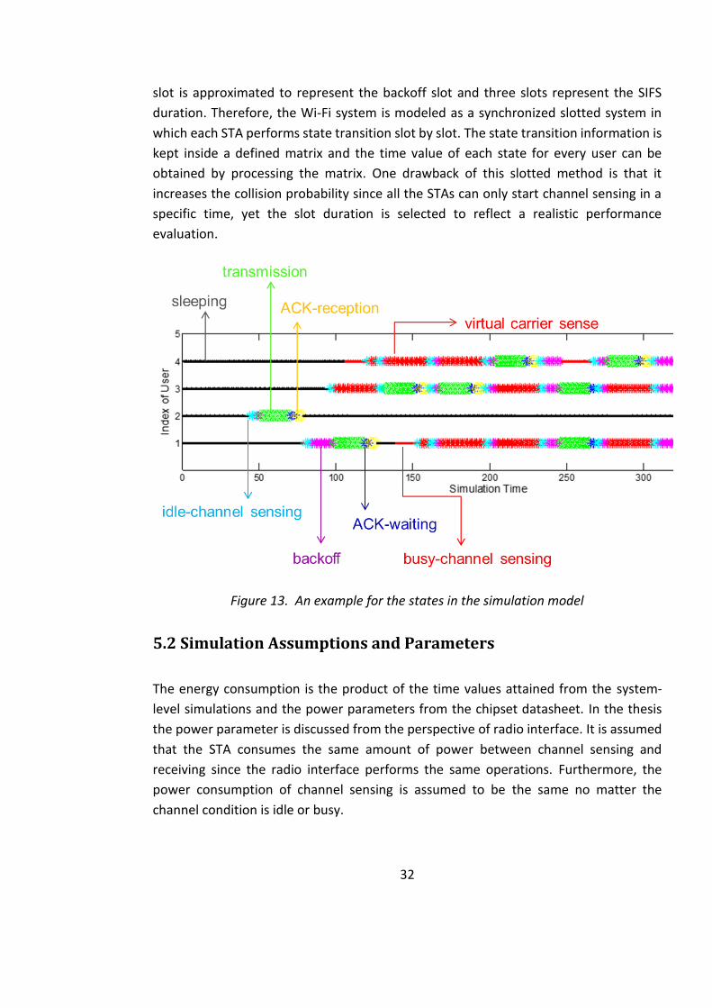
32

slot is approximated to represent the backoff slot and three slots represent the SIFS

duration. Therefore, the Wi-Fi system is modeled as a synchronized slotted system in

which each STA performs state transition slot by slot. The state transition information is

kept inside a defined matrix and the time value of each state for every user can be

obtained by processing the matrix. One drawback of this slotted method is that it

increases the collision probability since all the STAs can only start channel sensing in a

specific time, yet the slot duration is selected to reflect a realistic performance

evaluation.

Figure 13. An example for the states in the simulation model

5.2 Simulation Assumptions and Parameters

The energy consumption is the product of the time values attained from the system-

level simulations and the power parameters from the chipset datasheet. In the thesis

the power parameter is discussed from the perspective of radio interface. It is assumed

that the STA consumes the same amount of power between channel sensing and

receiving since the radio interface performs the same operations. Furthermore, the

power consumption of channel sensing is assumed to be the same no matter the

channel condition is idle or busy.

33

As shown in Table 5, chipset power consumption values in different modes, such as

transmission, reception, channel sensing are taken from 802.11n [33], whereas the

values for the sleeping mode are taken from 802.15.4 chipset [34]. It is assumed that

the sleeping power consumption in 802.11ah could go down to the level of 802.15.4

with the introduced enhancements and anticipated chipset optimizations.

Table 5. STA Power consumption values in different modes.

Mode Power (mW)

Data transmission 255

Data reception 135

Channel sensing 135

Sleeping 0.036

Table 6. Main simulation assumptions (default).

Simulation time 600 s

PHY layer data rate 150 kbps

Number of STAs 288

Average inter-arrival time Poisson, 10 s

SIFS 160 μs

AIFS Sensor STA: 264 μs

Non-Sensor STA: 316 μs

CWmin Sensor STA: 4

Non-Sensor STA: 16

CWmax Sensor STA: 16

Non-Sensor STA: 1024

Backoff slot 52 μs

DTIM interval 60 s

DTIM beacon length 102 bytes

Data length 134 bytes

ACK length 14 bytes

Maximum number of retransmissions

7

To figure out the fundamental reason of the energy consumption, the event is analyzed

in data transmission and reception, and channel sensing based on Wi-Fi standards [6].

For the data transmission mode, successful transmission and retransmission (due to

packet collision) are taken into account. In the data reception mode, the ACK-waiting

and ACK/beacon-reception are included since it is assumed that downlink traffic is not

used in the simulation modelling. Finally, the channel sensing is assumed to include idle-

34

channel listening, busy-channel listening, backoff, physical (PHY) header decoding

failure and virtual carrier sensing (VCS).

To evaluate the performance, 802.11ah MAC layer is modeled with 802.11ah

parameters illustrated in Table 6. The physical layer is assumed ideal as the impact of

MAC parameters on the system performance is particularly analyzed. It is also assumed

that the physical layer data rate is set up to be 150kbps which is the lowest rate

supported by the 802.11ah physical layer. The hidden node problem is not considered

and CTS/RTS is not deployed since the identical small data size is utilized for each STA.

In the simulator, a test scenario is modeled which is based on an agriculture and farming

use case. The scenario parameters, for example, the number of STAs and inter-arrival

time, are selected to reflect a similar channel occupancy ratio as in [19], yet with a less

number of STAs and a shorter inter-arrival time comparatively. Thus, more number of

data packet transmissions per STA can be observed in the given simulation time, 600 s.

The scenario is modeled with sporadic data traffic based on Poisson arrival.

35

6 Simulation Results

6.1 Impact of TIM Segmentations

To analyze the system performance against different TIM segmentations, the system-

level evaluations are carried out for different number of TIM groups, which are 1, 2, 4,

6 and 8, keeping the DTIM interval fixed (60 s). Therefore, in the evaluations, TIM beacon

interval is inversely proportional to the number of TIM groups. For the selected use case,

the total number of users is assumed to be 288. Each user generates uplink data packets

following Poisson process, which is widely used for modeling wireless data traffic [35],

with an average inter-arrival time of 10 s. It is assumed there is a single traffic type in

the simulation which is best effort mapping to EDCA access category [6]. Following the

impact of the TIM segmentation is evaluated for S-STA and NS-STA parameters

respectively.

6.1.1 Sensor Type EDCA Parameters

In this part, the EDCA parameter type is assumed to be the S-STA. In this case, the

minimum and maximum values of the contention window are 4 and 16 respectively

while the AIFS has the same duration as DIFS [6].

As shown in Figure 14, where the red and blue curves refer to the channel occupancy

and collision probability respectively, both collision probability and channel occupancy

broadly vary with the number of TIM groups. The collision probability is considerably

small for TIM deployment with one group. This is because TIM segmentations cause the

STA having buffered packets which are sent simultaneously in the beginning of each TIM

interval. Furthermore, when the number of TIM groups grows, the collision probability

increases since the packets are more likely to buffered and transmitted simultaneously

in the beginning of the TIM interval. However, the collision probability then slightly

decreases since with the increase in the TIM segmentation, the number of STAs in each

group decreases and the number of simultaneous competing STAs reduces thereof.

For single TIM group setting, through the considerably small collision probability, it can

be inferred that roughly all the generated packets can individually occupy the channel.

When the number of TIM groups is more than one, channel occupancy first drops, then

increases. This is because that competition among STAs are restricted into the certain

segments; however when the segmentation increases, the number of queued packets

36

that are to be sent simultaneously increases as well. Thus, these packets experiences

higher channel congestion and larger number of retransmissions.

Figure 14. Collision probability and channel occupancy vs. TIM segmentation (no RAW implementation). Sensor-type EDCA parameters are assumed.

In order to evaluate the packet delivery condition, the packet delivery ratio is defined to

be the percentage of the packets successfully transmitted. Accordingly, the packet

discard and buffer ratios are defined as the percentage of the packets discarded and

remained in the buffer.

Figure 15 shows the packet delivery conditions. For TIM deployment with one group, all

the packets can successfully be transmitted while more than half of the generated

packets cannot be delivered when the number of TIM groups increases. Also, it can be

observed that the variation of packet delivery ratio is largely correlated with the packet

discard ratio. Furthermore, the impact of TIM segmentation on discard ratio is the same

as that on collision probability because discard ratio is proportional to the collision

probability. In addition, the packet buffer ratio slightly increases when the number of

TIM segmentation grows since the packets are more likely to arrive after the last access

to the TIM interval in case of sporadic data traffic.

In order to understand the energy cost behavior of an STA during the channel access,

the energy consumption is decomposed according to status of the STA. Successful

transmission indicates the energy spent in data transmission without any collision while

retransmission refers to the energy spent due to collisions. ACK/beacon-reception

1 2 4 6 80

0.1

0.2

0.3

0.4

0.5

0.6

0.7

0.8

0.9

1

Total Number of TIM Groups

Channel Occupancy

Collision Probability

37

denotes the energy spent on receiving ACK and beacon frame while ACK-waiting

indicates the energy consumption of carrier sensing while waiting for ACK. Idle-channel

sensing and backoff refer to the energy consumed on DIFS sensing and backoff

procedure respectively in an idle channel. Channel sensing under a busy channel is

decomposed into three parts including PHY header decoding failure, busy-channel

sensing and VCS. If an STA wakes up and senses the channel busy, it has to sense the

channel until it becomes idle again. Busy-channel sensing denotes the energy spent in

this period of busy time. During carrier sensing, an STA can perform virtual carrier

sensing once it successfully decodes the PHY header of the packet transmitting in the

channel. Therefore, virtual carrier sense is used to represent the energy of decoding the

PHY header during this procedure. However, an STA cannot perform virtual carrier

sensing if it cannot decode the PHY header because of collision. In this case, the STA has

to listen to this collided channel until it is idle. PHY header decoding failure shows the

energy cost in this period.

Figure 15. Packet delivery condition vs. TIM segmentation (no RAW implementation). Sensor-type EDCA parameters are assumed.

Figure 16 shows the average energy consumption per STA in each status. For TIM

deployment with one group, the energy consumption is significantly small. As a

comparison, STAs consumes larger amount of energy for TIM deployment with more

than one group. This is because that TIM restriction for uplink channel access leads to

simultaneous channel access attempts among TIM STAs. Therefore, they waste large

amount of energy, especially due to retransmissions and PHY header decoding failures.

1 2 4 6 80

0.1

0.2

0.3

0.4

0.5

0.6

0.7

0.8

0.9

1

Total Number of TIM Groups

Delivery Ratio

Discard Ratio

Buffer Ratio

38

All in all, it is straightforward to make a statement that for sporadic traffic, STAs cannot

benefit from the TIM segmentation using sensor parameters if the traffic is uplink

dominated.

Figure 16. Average energy consumption per device vs. TIM segmentation (no RAW implementation). Sensor-type EDCA parameters are assumed.

Yet, it is essential to analyze the impact of sensor parameters before making a final

conclusion. When sensor-type EDCA parameters are used, the initial CW size is four, thus

around one quarter of STAs will generate backoff counter 0 and attempt to transmit

data simultaneously. Therefore, these transmissions from one quarter of STAs will

collide with each other resulting in PHY header decoding failures for the rest of TIM STAs.

Based on the observations from the simulations, this will repetitively continue and cause

additional energy consumption. Therefore, it is important to analyze the TIM

segmentation behavior with different EDCA parameters e.g., non-sensor type EDCA

parameters as will be discussed in the following section.

6.1.2 Non-Sensor Type EDCA Parameters

In this part, the traffic type is assumed to be the NS-STA best effort mapping to the EDCA

access category. In this setting, the minimum and maximum of the contention window

is 16 and 1024 respectively while the AIFS has a slightly longer duration than DIFS [6].

1 2 4 6 80

0.5

1

1.5

2

2.5

En

erg

y P

er

De

vic

e [J]

Total Number of TIM Groups

Successful Transmission

Retransmission

ACK/Beacon-Reception

ACK-Waiting

Backoff

Idle-Channel Sensing

PHY Header Decoding Failure

Busy-Channel Sensing

Virtual Carrier Sense

Sleeping

39

Figure 17. Collision probability and channel occupancy vs. TIM segmentation (no RAW

implementation). Non-sensor-type EDCA parameters are assumed.

In Figure 17, the red and blue curves refer to the channel occupancy and collision

probability respectively. The collision probability is expectedly small for TIM deployment

with one group as in Figure 14 since simultaneous transmission probability is lower.

Compared with Figure 14, NS-STA EDCA parameter configuration results in a lower

collision probability than that in S-STA EDCA parameters. This is because STA with NS-

STA parameter configuration utilizes larger CW to access the channel which has better

ability of collision avoidance.

As illustrated by red curve in Figure 17, with the increase of the number of the TIM

groups, the channel occupancy increases, similarly to Figure 14, since the simultaneous

transmissions caused by TIM segmentation cause high collision and increase the

retransmission time. Furthermore, the trend of collision probability then keeps constant

since the collision probability does not change much as the number of TIM segmentation

grows.

Figure 18 shows the packet delivery status in case of NS-STA EDCA parameter

configuration. Same as the S-STA case, all the packets are successfully transmitted for

TIM deployment with one group without any restriction of the channel access. By means

of the large CWs utilized in NS-STA EDCA parameter, the discard ratio is considerably

small even though the number of the TIM segmentation is increased. In addition, the

packet buffered ratio slightly increases since the packets are more likely to arrive after

1 2 4 6 80

0.1

0.2

0.3

0.4

0.5

0.6

0.7

Total Number of TIM Groups

Channel Occupancy

Collision Probability

40

the final access TIM interval. The buffered packets which are pending to be transmitted

are the reason of delivery level below 1.

Figure 18. Packet delivery condition vs. TIM segmentation (no RAW implementation). Non-sensor-type EDCA parameters are assumed.

Figure 19. 50%-ile and 90%-ile delay vs. TIM segmentation (no RAW implementation). Non-sensor-type EDCA parameters are assumed.

1 2 4 6 80

0.1

0.2

0.3

0.4

0.5

0.6

0.7

0.8

0.9

1

Total Number of TIM Groups

Delivery Ratio

Discard Ratio

Buffer Ratio

1 2 4 6 80

5

10

15

20

25

30

35

40

45

50

Total Number of TIM Groups

90

% D

ela

y [s]

50%-ile Delay

90%-ile Delay

41

Figure 19 shows both the 50 and 90 percentiles of the cumulative distribution function

(CDF) of the delay for non-sensor parameter deployment. The delay is only considered

for the packets which are successfully transmitted and it is calculated from the time of

generating a packet to the time of successfully delivering the packet. The delay can result

from the packet buffering or the time needed for the channel access, transmission and

retransmission.

As illustrated in Figure 19, both the 50 and 90 percentile delays are considerable small

for TIM deployment with one group since the packets can almost be immediately

transmitted with a very small collision probability. However, when there is a

segmentation, especially the 90 percentile delay is getting significantly longer despite

the larger CW configured via NS-STA EDCA parameter selection.

Figure 20. Average energy consumption per device vs. TIM segmentation (no RAW implementation). Non-sensor-type EDCA parameters are assumed.

Figure 20 shows the average energy consumption per device for NS-STA EDCA

parameter configuration. For TIM deployment with one group, the energy consumption

is considerably small and STA does not waste much energy in channel sensing. As a

comparison, in case of TIM segmentation with more than one group, STA consumes

larger amount of energy due to channel sensing as well as PHY header decoding failure.

This is because that transmissions from a large number of STAs are simultaneously

initiated at the beginning of each TIM interval when there are multiple TIM groups. Yet,

the energy consumption decreases as the TIM segmentation grows further e.g., with

1 2 4 6 80

0.5

1

1.5

2

2.5

3

3.5

En

erg

y P

er

De

vic

e [J]

Total Number of TIM Groups

Successful Transmission

Retransmission

ACK/Beacon-Reception

ACK-Waiting

Backoff

Idle-Channel Sensing

PHY Header Decoding Failure

Busy-Channel Sensing

Virtual Carrier Sense

Sleeping

42

respect to TIM deployment with two groups since the number of the simultaneously-

competing STAs is reduced.

The STAs that are configured with the CW parameter from the NS-STA EDCA parameter

set still consumes large amount of energy due to PHY header decoding failure. This is

because when a large number of STAs compete to access the channel at the same time,

1/16 of the STAs wound generate backoff counter zero and transmit simultaneously.

These STAs collide with each other while the remaining STAs fail to decode the PHY

header as a result of the collisions. This problem can be solved after the CW size is

enlarged sufficiently proportional to the total number of competing STAs.

6.2 Parameter Optimization

6.2.1 Additional Sleeping Cycles

In this part, a solution called additional sleeping (AS) cycles is proposed to minimize the

energy consumption in 802.11ah, especially the energy spent in channel sensing. The

fundamental mechanism of AS is that the STA intelligently moves to the sleeping state

instead of sensing the channel once it senses the channel busy. This additional sleeping

time is based on the sleeping window of each STA. Every time an STA goes into additional

sleeping cycle, it generates a random sleeping value which is uniformly distributed in

[SWmin, SWmax] where SWmin and SWmax represents the minimum and maximum

values of sleeping window respectively. AS cycles can be adjusted based on the channel

occupancy condition. Thus, the STA can generate larger sleeping windows if the data

traffic is high while this window size can be reduced once the traffic alters to lower state.

The channel occupancy or load is represented by L which indicates the percentage of

busy channel. T{busy} is defined to represent the mean value of channel busy time and

it equals to T{data packet} + T{SIFS} + T{ACK}, where T{data packet} is the average packet

length. Each STA can set up its sleeping window according to L and T{busy} and one

example can be SWmin = T{busy}*(1-L) and SWmax = T{busy}*(1+L). It is assumed that

the traffic occupancy information, L and average packet length T{data packet} are

contained in each of beacon frame so that TIM STAs can adjust their sleeping window

according to the channel condition. It should be note that for especially the delay-

sensitive service, the system ought to limit the maximum number of attempts of

additional sleeping.

The AS mechanism can work with VCS or without VCS. Once the STA identify the channel

moves from idle state to busy state, it can first try to decode the PHY header to perform

43

virtual carrier sensing. If it fails to decode the header, it can move to the AS mode to

save energy. The STA can also ignore the VCS mechanism by directly shifting into the AS

mode once it detects that the channel is busy. It is noteworthy that STA cannot perform

VCS if it wakes up during the transmission of another STA and in this case it can move to

the AS mode immediately. In the thesis, the AS mechanism is assumed to be activated

only when the STA wakes up in the middle of another transmission.

The number of TIM groups is selected to be one as it performs sufficiently well in terms

of energy-consumption in uplink as discussed in the earlier section. The EDCA

parameters are selected based on the best effort access category for both S-STA and NS-

STA. Their impact on the energy consumption is compared in addition to the AS solution.

In the parameter setting of AS solution, the sleeping window of each STA is fixed where

SWmin and SWmax equal to 6 and 12 ms respectively.

Figure 21. Energy consumption in case of sporadic uplink traffic in 10 minutes

Figure 21 shows that NS-STA parameters results in slightly more energy consumption

with respect to S-STA parameters. This is because NS-STA parameters dictate larger CW

when competing for the channel, thereby extends the channel sensing time (due to

larger backoff period). Even though larger CW reduces the energy consumption by

minimizing retransmissions, thanks to reduced collision probability, the gain is still

negligible for the modeled traffic scenario. As observed from Figure 21, the proposed AS

mechanism can save almost all the energy spent during the busy-channel sensing as the

STA can sleep during the most of this period. Moreover, the AS mechanism can reduce

S-STA par. NS-STA par. S-STA par. + AS0

20

40

60

80

100

120

140

160

En

erg

y P

er

De

vic

e [m

J]

Successful Transmission

Retransmission

ACK/Beacon-Reception

ACK-Waiting

Backoff

Idle-Channel Sensing

PHY Header Decoding Failure

Busy-Channel Sensing

Virtual Carrier Sensing

Sleeping

44

the collision probability by means of added randomness to the sleeping time and

minimizes the energy spent for retransmissions.

Figure 22. Collision probability and channel occupancy in case of sporadic uplink traffic

Figure 23. Delay in the case of sporadic uplink traffic

Figure 22 shows that the EDCA parameters do not affect much on the channel occupancy

for the modeled traffic scenario. This is because the collision probability in case of S-STA

parameter setting is already considerably small and larger CW dictated by NS-STA

Sensor par. Non-Sensor par. Sensor par. with AS0

0.02

0.05

0.1

0.15

0.2

Collision Probability

Channel Occupancy

Sensor par. Non-Sensor par. Sensor par. with AS0

2

4

6

8

10

12

14

16

18

20

De

lay [m

s]

90%-ile Delay

50%-ile Delay

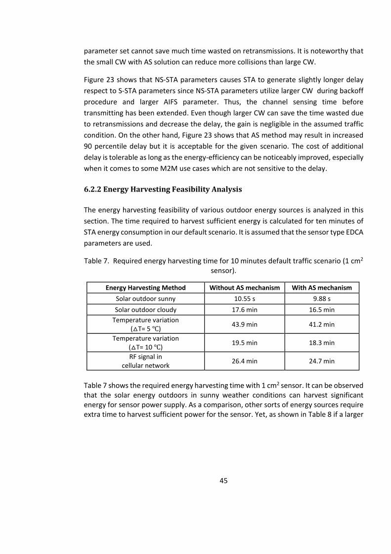
45

parameter set cannot save much time wasted on retransmissions. It is noteworthy that

the small CW with AS solution can reduce more collisions than large CW.

Figure 23 shows that NS-STA parameters causes STA to generate slightly longer delay

respect to S-STA parameters since NS-STA parameters utilize larger CW during backoff

procedure and larger AIFS parameter. Thus, the channel sensing time before

transmitting has been extended. Even though larger CW can save the time wasted due

to retransmissions and decrease the delay, the gain is negligible in the assumed traffic

condition. On the other hand, Figure 23 shows that AS method may result in increased

90 percentile delay but it is acceptable for the given scenario. The cost of additional

delay is tolerable as long as the energy-efficiency can be noticeably improved, especially

when it comes to some M2M use cases which are not sensitive to the delay.

6.2.2 Energy Harvesting Feasibility Analysis

The energy harvesting feasibility of various outdoor energy sources is analyzed in this

section. The time required to harvest sufficient energy is calculated for ten minutes of

STA energy consumption in our default scenario. It is assumed that the sensor type EDCA

parameters are used.

Table 7. Required energy harvesting time for 10 minutes default traffic scenario (1 cm2 sensor).

Energy Harvesting Method Without AS mechanism With AS mechanism

Solar outdoor sunny 10.55 s 9.88 s

Solar outdoor cloudy 17.6 min 16.5 min

Temperature variation (△T= 5 ℃)

43.9 min 41.2 min

Temperature variation (△T= 10 ℃)

19.5 min 18.3 min

RF signal in cellular network

26.4 min 24.7 min

Table 7 shows the required energy harvesting time with 1 cm2 sensor. It can be observed that the solar energy outdoors in sunny weather conditions can harvest significant energy for sensor power supply. As a comparison, other sorts of energy sources require extra time to harvest sufficient power for the sensor. Yet, as shown in Table 8 if a larger

46

harvesting area, e.g., 2 cm2, is used, other energy sources such as temperature variation could be sufficient as well.

Table 8. Required energy harvesting time for 10 minutes default traffic scenario (2 cm2 sensor).

Energy Harvesting Method Without AS mechanism With AS mechanism

Solar outdoor sunny 5.275 s 4.94 s

Solar outdoor cloudy 8.8 min 8.25 min

Temperature variation (△T= 5 ℃)

21.95 min 20.6 min

Temperature variation (△T= 10 ℃)

9.75 min 9.15 min

RF signal in cellular network

13.2 min 12.35 min

6.2.3 Impact of Traffic Load and Sleeping Window Size

In order to deeply evaluate the performance of the AS mechanism in different traffic

conditions, three traffic load states are selected. The traffic load states are represented

by the average packet inter-arrival rate of 10, 5 and 4 seconds, respectively. For each

traffic load state, small and large window sizes are simulated. The minimum and

maximum values of small SW are selected as 6 ms and 8 ms respectively, while these

values are extended to 6 ms and 12 ms for large SW. The EDCA parameters are selected

based on the sensor STA with best effort traffic type assumption in all the following

simulated cases.

The grayscale colormap is used for the illustration of results in this section. In each

figure, x axis shows the sleeping window size where VCS represents the case without

additional sleeping mechanism. Small SW and large SW indicate the cases with the AS

mechanism with small and large windows respectively. Y axis shows the traffic load

which is represented by packet inter-arrival time of 10 s, to 5 s and 4 s.

Figure 24 compares the collision probability in different traffic load conditions and for a

set of sleeping window sizes. The AS mechanism decreases the collision probability since

STAs are less likely to access the channel simultaneously by sleeping a random time.

Furthermore, the large sleeping window reduces collision probability more than small

window size since it contributes to more randomness. In a traffic scenario with the inter-

arrival time of 4 s (high traffic load), the collision probability is considerably large (over

80%) while the gain of collision avoidance by the AS mechanism is significantly high. As

47

a comparison, the improvement on the collision avoidance in lower traffic load is not

obvious.

Figure 24. Collision probability vs. traffic load and additional sleeping parameters

Figure 25. 90 percentile delay vs. traffic load and additional sleeping parameters

Inte

rarr

iva

l T

ime

[s]

Average Collision Probability

VCS Small SW Large SW

10

5

4

0.1

0.2

0.3

0.4

0.5

0.6

0.7

0.8

Inte

rarr

iva

l T

ime

[s]

90%-ile Delay [s]

VCS Small SW Large SW

10

5

4

0.05

0.1

0.15

0.2

0.25

0.3

48

Figure 25 shows the 90 percentile delay. In the lower traffic load, for instance, 10 s and

5 s inter-arrival rate, the AS mechanism increases the delay since in this case the delay

caused by retransmission is negligible compared with the delay added by additional

sleeping cycles. Furthermore, large sleeping window results in a larger delay due to the

longer sleeping time.

However, in case of higher traffic load with the inter-arrival time of 4 s, the AS

mechanism can decrease the 90 percentile delay since in this case the 90 percentile

delay mostly results from retransmissions. The delay cost in additional sleeping is

negligible compared with the delay saved by retransmission reduction. In this case, large

sleeping window can decrease the delay more than the small one through reducing

more collisions.

Figure 26. Average active energy consumption per packet vs. traffic load and

additional sleeping parameters

Figure 26 illustrates how much energy is spent in active mode in order to transmit one

packet successfully. It is assumed that the energy in sleeping mode is negligible

compared with that in active mode. In the higher traffic load which has the inter-arrival

rate of 4 s, the AS mechanism can save energy considerably since in this case STAs spend

much larger amount of energy in retransmissions. The benefit of AS mechanism is not

significant for lower traffic load conditions.

Inte

rarr

iva

l T

ime

[s]

Average Active Energy per Packet [mJ]

VCS Small SW Large SW

10

5

4

10

20

30

40

50

60

49

7 Conclusions

M2M communications have been anticipated to be the one of the driven force for the

future development of wireless technologies. The distinct features of M2M brings new

challenges for the design of wireless systems. Recently, in order to increase the

competence in future M2M market, several enhancements have been proposed in

different wireless technologies. For example, 3GPP has proposed several enhancements

for M2M applications in the latest releases, such as Release 12 and 13. In the area of Wi-

Fi, a new amendment named 802.11ah has been proposed accordingly.

The thesis briefly introduces the M2M enhancements in different wireless technologies

with a focus on 802.11ah technology. The scope is to evaluate the energy efficiency of a

new M2M enhancement proposed in 802.11ah known as TIM segmentations. The TIM

segmentation is a periodical channel access mechanism to efficiently group devices and

save energy. In order to thoughtfully understand the principle of this enhancement,

some fundamental MAC layer functions in Wi-Fi have been discussed. The methodology

utilized for performance evaluation is system-level Matlab simulation. The simulator is

based on state machine transition which models the behavior of 802.11ah MAC layer. It

focuses on uplink traffic following Poisson process assuming an agricultural scenario. In

addition, the thesis proposed an energy saving solution based on additional sleeping

(AS) cycles. In this method, the STA can smartly move to the sleep state instead of

wasting energy on channel sensing as soon as it identifies that the channel is likely to be

busy.

According to the simulation results, the TIM segmentation of channel access among

devices can deteriorate uplink transmission performance in case of sporadic data traffic.

This is because that TIM restriction in uplink increases the probability of simultaneous

transmissions among a large number of devices and this increases the collision

probability. Results shows that energy consumption is optimal when there is only one

TIM group (no access restriction). Adding more TIM group segmentations (2 to 8) can

increase the energy cost more than ten times. The observation is valid for both sensor

and non-sensor type EDCA parameter settings. The performance of AS mechanism has

also been evaluated for various traffic load conditions. The results show that AS

mechanism can save around 7% energy in low traffic load condition by introducing a

tolerable delay in channel access. The gain is even larger for higher traffic load

conditions.

The reason why TIM grouping in uplink deteriorates the performance is the CSMA/CA

mechanism. The random access procedure in CSMA/CA may not efficiently cope with

50

simultaneous access of a large number of devices. This may be solved by setting a

suitable initial size of contention window if the total number of access devices is known

in advance. However, in most cases, this number cannot be known so devices have to

initialize the channel access with the minimum contention window and gradually

increases the size after obtaining the collision feedback by the AP.

On the other hand, the grouping mechanism for uplink access may work in LTE systems.

In LTE, when a large number of devices access the channel in the same RA slot, they are

required to first send a preamble to eNodeB. The preamble is selected randomly from

an orthogonal sets, typically 54 numbers. The orthogonality enables eNodeB to detect

different preambles. If multiple devices select the same preamble simultaneously, a

collision will occur. The eNodeB may detect the collision based on the different arrival

time of the same preambles and broadcast a backoff indicator for the collided devices.

The advantages of LTE over Wi-Fi is that these collided devices can perform backoff

based on this indicator so they can identify the exact suitable time for the next access

retry. However, the drawback is that eNodeB may not able to detect the collision since

it may receive the same preambles constructively from the devices at the same place.

In this case, these devices will continue to collide with each other in the next

transmission.

The related research results, where the focus is on the RAW configuration, have also

been submitted as a conference paper [36]. Future work may consider downlink data

traffic along with uplink traffic, as well as the physical layer implementation in details.

Other MAC features such as Non-TIM operation and hidden node problem solutions can

also be considered.

51

References

[1] Machina Research, “M2M application characteristics and their implications for

spectrum,” white paper 2606/OM2M/FR/V2, May 2014.

[2] Ericsson, “LTE Release 13,” white paper Uen 284 23-8267, April 2015.

[3] Nokia, “LTE-Advanced Evolution in Release 12 – 14; New services to pave the way

to 5G,” white paper, 2015.

[4] Nokia, “Nokia LTE M2M; Optimizing LTE for the Internet of Things,” white paper,

2014.

[5] 3GPP, “LTE; General Packet Radio Service (GPRS) enhancements for Evolved

Universal Terrestrial Radio Access Network (E-UTRAN) access,” TS 23.401,

September 2014.

[6] IEEE Standard Association, “Wireless LAN Medium Access Control (MAC) and

Physical Layer (PHY) Specifications: Amendment 6: Sub 1 GHz License Exempt

Operation,” P802.11ah/D0.1, May 2014.

[7] A. Osseiran, F. Boccardi, V. Braun, K. Kusume, P. Marsch, M. Maternia, and M.

Fallgren, “Scenarios for 5G mobile and wireless communications: the vision of the

METIS project,” IEEE Communications Magazine, vol. 52, no. 5, May 2014.

[8] O. N. C. Yilmaz, “5G radio access for ultra-reliable and low-latency

communications,” Ericsson Research Blog, May 2015.

[9] R. Ratasuk, A. Prasad, Z. Li, A. Ghosh, and M.A. Uusitalo, “Recent advancements in

M2M communications in 4G networks and evolution towards 5G,” IEEE

Conference on Intelligence in Next Generation Networks, pp. 52-57, February

2015.

[10] C. S. Bontu and E. Illidge, “DRX mechanism for power saving in LTE,” IEEE

Communications Magazine, vol. 47, no. 6, June 2009.

[11] S. C. Jha, A. T. Koc, M. Gupta, and R. Vannithamby, “Power saving mechanisms for

M2M communication over LTE networks,” IEEE Conference on Communications

and Networking, pp. 102-106, July 2013.

[12] 3GPP, “Study on RAN Improvements for Machine-Type Communications,” TR

37.868, September 2011.

[13] A. Laya, L. Alonso, and J. Alonso-Zarate, “Is the random access channel of LTE and

LTE-A suitable for M2M communications? A survey of alternatives,” IEEE

Communications Surveys & Tutorials, vol. 16, no.1, February 2014.

[14] IEEE Standard Association, “Wireless LAN Medium Access Control (MAC) and

Physical Layer (PHY) Specifications,” April 2012.

[15] J. Lansford, A. Stephens, and R. Nevo, “Wi-Fi (802.11 b) and Bluetooth: enabling

coexistence,” IEEE Journals on Network, vol. 15, no. 5, October 2001.

52

[16] Bluetooth Special Interest Group, “Bluetooth Core Specification Version 4.0,” June

2010.

[17] Bluetooth Special Interest Group, “Bluetooth Core Specification Version 4.1,”

December 2013.

[18] Bluetooth Special Interest Group, “Bluetooth Core Specification Version 4.2,”

December 2014.

[19] T. Adame, A. Bel, B. Bellalta, J. Barcelo, and M. Oliver, “IEEE 802.11 AH: the WiFi

approach for M2M communications,” IEEE Journal on Wireless Communications,

vol. 21, no. 6, December 2014.

[20] W. Sun, M. Choi, and S. Choi, “IEEE 802.11 ah: A long range 802.11 WLAN at sub 1

GHz,” Journal of ICT Standardization, vol. 1, no. 1, May 2013.

[21] L. Zheng, M. Ni, L. Cai, J. Pan, C. Ghosh, and K. Doppler, “Performance analysis of

group-synchronized DCF for dense IEEE 802.11 networks,” IEEE Transactions on

Wireless Communications, vol. 13, no. 11, July 2014.

[22] S. J. Roundy, “Energy scavenging for wireless sensor nodes with a focus on

vibration to electricity conversion,” PhD thesis, University of California, Berkeley,

2003.

[23] J.A. Paradiso and M. Feldmeier, “A compact, wireless, self-powered pushbutton

controller,” ACM Conference on Pervasive and Ubiquitous Computing, pp. 299-

304, October 2001.

[24] S. Kahrobaee, and M. C. Mehmet, “Vibration energy harvesting for wireless

underground sensor networks,” IEEE ICC, pp. 1543-1548, June 2013.

[25] Y. K. Tan and S. K. Panda, “Review of energy harvesting technologies for

sustainable wireless sensor network,” IEEE Conference on Communication

Technology, pp. 362-367, September 2011.

[26] T. Le, K. Mayaram and T. Fiez, “Efficient far-field radio frequency energy harvesting

for passively powered sensor networks,” IEEE Journal on Solid-State Circuits, vol.

43, no. 5, May 2008.

[27] H. Nishimoto, Y. Kawahara, and T. Asami, “Prototype implementation of ambient

RF energy harvesting wireless sensor networks,” IEEE Conference on Sensors, pp.

1282-1287, November 2010.

[28] A. M. Zungeru, L. M. Ang, S. Prabaharan, and K. P. Seng, “Green Mobile Devices

and Networks: Energy Optimization and Scavenging Techniques,” CRC Press, 2012.

[29] H. Nakamoto, D. Yamazaki, T. Yamamoto, H. Kurata, S. Yamada, K. Mukaida and K.

Gotoh, “A passive UHF RF identification CMOS tag IC using ferroelectric RAM in

0.35-μm technology,” IEEE Journal on Solid-State Circuits, vol. 42, no. 1, January

2007.

53

[30] G. Bianchi, “Performance analysis of the IEEE 802.11 distributed coordination

function,” IEEE Journal on Selected Areas in Communications, vol. 18, no. 3, March

2000.

[31] M. Ergen and P. Varaiya, “Decomposition of energy consumption in IEEE 802.11,”

IEEE ICC, pp. 403-408, June 2007.

[32] P. Serrano, A. Garcia-Saavedra, M. Hollick, and A. Banchs, “On the energy

efficiency of IEEE 802.11 WLANs,” IEEE Conference on Wireless, pp. 932-939, April

2010.

[33] O. Raeesi, J. Pirskanen, A. Hazmi, T. Levanen, and M. Valkama, “Performance

evaluation of IEEE 802.11 ah and its restricted access window mechanism,” IEEE

ICC, pp. 460-466, June 2014.

[34] Texas Instruments, CC2420 datasheet.

[35] O. N. C. Yilmaz, J. Hämäläinen and S. Hämäläinen, “Self‐optimization of random

access channel in 3rd Generation Partnership Project Long Term Evolution,”

Journal of Wireless Communications and Mobile Computing, vol. 11, no. 12,

November 2011.

[36] Z. Yue, O. N. C. Yilmaz, A. Larmo, “Optimizing M2M energy-efficiency in IEEE

802.11ah,” ISWCS, August 2015 (Submitted).