Analysis of explicit and implicit discrete-time equivalent

HAL Id: hal-00875209https://hal.inria.fr/hal-00875209

Submitted on 21 Oct 2013

HAL is a multi-disciplinary open accessarchive for the deposit and dissemination of sci-entific research documents, whether they are pub-lished or not. The documents may come fromteaching and research institutions in France orabroad, or from public or private research centers.

L’archive ouverte pluridisciplinaire HAL, estdestinée au dépôt et à la diffusion de documentsscientifiques de niveau recherche, publiés ou non,émanant des établissements d’enseignement et derecherche français ou étrangers, des laboratoirespublics ou privés.

Analysis of explicit and implicit discrete-timeequivalent-control based sliding mode controllers

Olivier Huber, Vincent Acary, Bernard Brogliato

To cite this version:Olivier Huber, Vincent Acary, Bernard Brogliato. Analysis of explicit and implicit discrete-timeequivalent-control based sliding mode controllers. [Research Report] RR-8383, INRIA. 2013, pp.23.�hal-00875209�

https://hal.inria.fr/hal-00875209

https://hal.archives-ouvertes.fr

ISS

N02

49-6

399

ISR

NIN

RIA

/RR

--83

83--

FR+E

NG

RESEARCHREPORTN° 8383October 2013

Project-Team BiPoP

Analysis of explicit andimplicit discrete-timeequivalent-control basedsliding mode controllersOlivier Huber, Vincent Acary, Bernard Brogliato

RESEARCH CENTREGRENOBLE – RHÔNE-ALPES

Inovallée655 avenue de l’Europe Montbonnot38334 Saint Ismier Cedex

Analysis of explicit and implicit discrete-timeequivalent-control based sliding mode

controllers

Olivier Huber, Vincent Acary, Bernard Brogliato

Project-Team BiPoP

Research Report n° 8383 — October 2013 — 23 pages

Abstract: Different time-discretization methods for equivalent-control based sliding mode control(ECB-SMC) are presented. A new discrete-time sliding mode control scheme is proposed for lineartime-invariant (LTI) systems. It is error-free in the discretization of the equivalent part of thecontrol input. Results from simulations using the various discretized SMC schemes are shown,with and without perturbations. They illustrate the different behaviours that can be observed.Stability results for the proposed scheme are derived.

Key-words: sliding mode control, sampled-data system, discrete-time Lyapunov stabil-ity,implicit discretization

Analyse de la discretization explicite ou implicite des controlleurs parmodes glissants

Résumé : Dans ce rapport, differentes techniques de discretisation temporelle pour le contrôle par modesglissants sont présentées. Une nouvelle structure de contrôle par modes glissants est proposée pour des systèmeslinéaires invariants. Elle ne comporte pas d’erreur dans la discretisation de la partie équivalente du contrôle. Desrésultats de simulations avec divers contrôlleurs par modes glissants sont présentées, avec ou sans perturbation. Ilsillustrent les phénomènes qui peuvent être observés suivant le type de discretisation utilisé. Pour finir, la stabilitéde la nouvelle structure de contrôle est étudiée.

Mots-clés : contrôle par modes glissants, système échantionnés, stabilité de Lyapunov en temps discret, discreti-sation implicite

Analysis of explicit and implicit discrete-time equivalent-control based sliding mode controllers 3

1 Introduction

The time discretization of sliding-mode controllers has witnessed an intense activity in the past 30 years [1–6]and [7]. This concerns in particular the classical Equivalent-Control-Based Sliding-Mode Control (ECB-SMC),which consists of two sub-controllers: the state-continuous equivalent control ueq and the state-discontinuous controlus. In these past research efforts, most of the focus was on the discontinuous part of the control, since it introducesnumerical chattering. Several solutions to alleviate numerical chattering (that is solely due to the time discretization[8–12]) have been proposed [1–7,13,14], most of them consisting in the definition of a so-called quasi-sliding surface [5]and an explicit discretization of us. The works in [2] and [6] depart from these discrete-time controllers and proposean algorithm which allows the sliding variable to take exactly the zero value at sampling times. They are howeverlimited to first order, scalar systems and require some stringent assumptions. Recently a new approach, which maybe seen as a (non-trivial) extension of the controllers in [2] and [6], has been proposed in [11] and [12]. The basicidea is to implement the discontinuous input us in an implicit form, while keeping its causality (i.e. the controlleris nonanticipative). Then this input has to be computed at each sampling time as the solution to a generalized,set-valued equation, which takes the form of a simple projection on an interval in the simplest cases. Let us illustratethe difference between explicit and implicit discretization with an academic example, x(t) ∈ −α sgn(x(t)), α > 0.We use the differential inclusion framework since we let sgn(0) to take any value in [−1, 1] (this is formally stated inDefinition 1 as Sgn). An explicit discretization yields x(tk+1) ∈ x(tk)−hα sgn(x(tk)), whereas the implicit one yieldsx(tk+1) ∈ x(tk)− hα sgn(x(tk+1)). As long as |x(tk)| � hα, there is no difference between the two discretizations.But if |x(tk)| < αh, then the behaviour changes with the type of discretization. With 0 < x(tk) < hα, in theexplicit case, x(tk+1) ∈ x(tk) − hα sgn(x(tk)) < 0. The sign of the state will change at every tk, leading to thewell-known chattering phenomenon. Whereas in the implicit case, it is possible to ensure x(tk+1) = 0 by choosingsgn(x(tk+1)) = x(tk)/(αh) < 1. The implicit discretization of the sign function is rigorously presented in Section 3.

To the best of our knowledge, the discretization of the equivalent part has received little attention. In this work,we present a study of the effects of discretization on both the equivalent and discontinuous part of the control.After studying the different discretization methods and their shortcomings, we propose a new discrete-time controlscheme, where the equivalent part is not a discretized version of its continuous-time counterpart but is directlydesigned from the discrete-time dynamics. Some properties of this scheme, like finite-time convergence to thesliding surface and perturbation attenuation, are studied in Section 7.

In this paper, we consider systems of the formx(t) = Ax(t) +Bu(t) +Bξ(t)

u(t) = ueq(t) + us(t)

σ(t) := Cx(t)

us(t) ∈ −α Sgn (σ(x(t))) ,

(1)

with x(t) ∈ Rn, u(t) ∈ Rp, σ(t) ∈ Rp, C ∈ Rp×n, and α > 0. The function σ is called the sliding variable, thedisturbance is denoted as ξ, and Sgn is formally introduced in Definition 1. The perturbation ξ is supposed to be atleast continuous: noise is not considered in this paper. When ξ = 0, the system is said to be nominal. The methodused to discretize the dynamics is called Zero-Order Hold (ZOH), also known as exact sampled-data representation.It is often considered for technological reasons, but also because there is no error with this discretization method.

In the remainder of this section, we introduce the notation. In Section 2 we briefly recall the ECB-SMC theory.Then some classical discretization methods are presented in Section 3. Section 4 is dedicated to the discreteerror analysis of various controllers of Section 3. We introduce our new discrete-time SMC scheme in Section 5.Simulation results using different time-discretization methods are shown in Section 6, to illustrate the possibledifferent behaviours of the closed-loop system. Finally, stability results are derived in Section 7. Conclusions endthe paper in Section 8.

Notations: Let x : R+×Rp×Rn → Rn be the solution of system (1), x := x( · , u, x0) is the solution associatedwith a continuous-time control u and an initial state x0 ∈ Rn, while x := x( · , u, x0) is the solution with a stepfunction u and the same initial state. In the latter case, we denote by σ := Cx the sliding variable. The controlvalues change at predefined time instants tk, defined for all k ∈ N : tk := t0 + kh, t0, h ∈ R+. The scalar h iscalled the timestep. We denote xk := x(tk) and σk := σ(tk) for all k ∈ N. For all y ∈ Rr, ‖y‖∞ = maxi |yi|. For allM ∈ Rr×s, ‖M‖∞ = maxi

∑j |Mij |. Let w : R→ Rr and S be any interval in R, ‖w‖∞,S = maxi ess supt∈S |wi(t)|.

Let 〈 · , · 〉 denote the standard inner product in a Euclidean space and ‖ · ‖ the norm based upon it. Let sgn be theclassical single-valued sign function: for all x > 0, sgn(x) = 1, sgn(−x) = −1 and sgn(0) = 0.

RR n° 8383

4 Olivier Huber, Vincent Acary, Bernard Brogliato

Definition 1 (Multivalued sign function). Let x ∈ R. The multivalued sign function Sgn: R ⇒ R is defined as:

Sgn(x) =

1 x > 0

−1 x < 0

[−1, 1] x = 0.

(2)

If x ∈ Rn, then the multivalued sign function Sgn: Rn ⇒ Rn is defined as: for all j = 1, . . . , n, (Sgn(x))j := Sgn(xj).

Definition 2. Let f : Rn × R→ Rp and l ∈ R. One has f = O(hl) if for all x ∈ Rn, there exists c ∈ Rp such thatf(x, h)/hl → c as h→ 0.

Definition 3. [15, p. 147] Let M ∈ Rn×n. M is a P-matrix if for all x ∈ Rn such that for all i ∈ {1, . . . , n},xi(Mx)i ≤ 0, then x = 0.

Lemma 1. [15, p. 147] Let M ∈ Rn×n. If M is positive-definite, then M is a P-matrix.

2 The equivalent-based continuous-time sliding-mode controller

Let us assume that the triplet (A,B,C) has a strict vector relative degree (1, 1, . . . , 1). This implies that thedecoupling matrix CB is full rank. The dynamics of the sliding variable in the nominal system (1) (that is withξ(t) = 0) is

σ(t) = CAx(t) + CBueq(t) + CBus(t). (3)

The control law ueq is designed such that the system stays on the sliding surface once it has been reached (in otherword ueq renders the sliding surface invariant with us ≡ 0):

σ(t) = 0 and us(t) = 0 ⇒ ueq(t) = −(CB)−1CAx(t). (4)

Then the sliding variable dynamics with the equivalent control reduces to{σ(t) = CBus(t)

us(t) ∈ −α Sgn(σ(t)).(5)

The nominal system (1) can be rewritten as

x(t) = (I −B(CB)−1C)Ax(t) +Bus(t), (6)

or equivalently

x(t) = ΠAx(t) +Bus(t), (7)

with Π := I − B(CB)−1C. Two interesting properties of Π are CΠ = 0 and Π is a projector [16]. Taking theintegral form of system (7) yields the relation

x(t) = Φ(t, t0)x(t0) +

∫ t

t0

Φ(t, τ)Bus(τ)dτ, (8)

with Φ(t, t0) = eΠA(t−t0) the state transition matrix for the system (7). Some of the properties of Φ are given inthe following lemma.

Lemma 2. One has Φ(t, t0) = ΠAΦ(t, t0), Φ(t0, t0) = I, and CΦ = C for all t ≥ t0.

Proof. One has CΦ(t, t0) = 0 so CΦ(t, t0) = CΦ(t0, t0) = C for all t ≥ t0.

Inria


3 Discrete-time controllers

3.1 Classical discretization methods to obtain discrete-time controllersFrom now on, ueq and us are sampled control laws defined as right-continuous step functions:

ueq(t) = ueqk , t ∈ [tk, tk+1) (9)us(t) = usk, t ∈ [tk, tk+1). (10)

The goal of the discretization process is to choose the elements of the sequences {ueqk } and {usk} such that thediscrete-time system exhibits properties as close as possible to the ones with a continuous-time controller. Incontinuous time, sliding-mode controlled systems have their evolution divided into two phases: the reaching phase,where ‖σ‖ > 0 and is decreasing, and the sliding phase, where σ = 0 and the sliding motion occurs. It is wellknown that the sliding motion does not occur in general in discrete time even on a nominal system because of theerror induced by the discretization. This has led to the definition of quasi-sliding surfaces [5]. By analogy with theFilippov’s solutions we define the following.

Definition 4 (Discrete-time sliding phase). A system (1), in its sampled-data form, is in the discrete-time slidingphase if us takes values in (−α, α)p.

Such a definition appears to be new in the discrete-time sliding mode control field since it implies that thediscrete-time discontinuous controller is itself set-valued, just as its continuous-time counterpart in (1) and (5).This will be made possible with an implicit implementation, as proved in [11] and [12]. It is crucial not to definethe sliding phase in terms of σk, but rather in terms of the discontinuous input us. In continuous-time, Definition 4applied to us implies that the system is in the sliding phase σ ≡ 0, see (5). It holds with a matched perturbationas long as for all t ≥ 0, ‖ξ(t)‖∞ ≤ δ < α for some δ ≥ 0.

Integrating the nominal version of (1) over [tk, tk+1) and using the expressions in (10), we obtain the ZOHdiscretization of the system:

xk+1 = eAhxk +B∗ueqk +B∗usk, (11)

with

B∗ :=

∫ tk+1

tk

eA(tk+1−τ)Bdτ. (12)

Let Ψ :=∫ tk+1

tkeA(tk+1−τ)dτ =

∑∞l=0

Alhl+1

(l+1)! , then B∗ = ΨB. We now present different choices for the values ueqk and

usk. Firstly, standard methods are described, while the new method is studied in the next section. Here ueqk and uskare the discretized values of the continuous-time control law ueq and us. From all the possible time-discretizationschemes, we focus on the one-step explicit, implicit, and midpoint ones. With the expressions found for ueq and usin (4) and (5), the proposed discretized values for the equivalent control ueqk are:

ueqk,e = −(CB)−1CAxk explicit input, (13a)

ueqk,i = −(CB)−1CAxk+1 implicit input, (13b)

ueqk,m = 1/2(ueqk,e + ueqk,i) midpoint input, (13c)

and the two possibilities for the discontinuous control usk are:

usk = −α sgn(σk) explicit input, (14a)usk ∈ −α Sgn(σk+1) implicit input. (14b)

We use the singled-valued sgn function in (14a) since the case σk = 0 is not worth considering for explicit inputs.Moreover with the set-valued Sgn function, if σk = 0, then we would have Sgn(σk) ∈ [−α, α]p and there is no properselection procedure to get a value for usk. In the next subsection, we present the selection procedure in the implicitcase. The objective in Section 6 is to study the behaviour of the closed-loop system when different combinations ofequations (13a)–(13c) and (14a)–(14b) are used. The most commonly used control law is the combination of (13a)and (14a). This kind of discretization has been studied in [8, 9, 17], with a focus on the sequence formed by σkonce the system state approaches the sliding manifold. The implicit discretization (14b) was first introduced in [11]and [12]. In the following, we provide more details on it.

RR n° 8383


3.2 Definition and properties of the implicitly discretized discontinuous control input

With the implicit method (14b), for each k ∈ N, usk is computed as the solution to the generalized equation{σk+1 = σk + CB∗uskusk ∈ −α Sgn(σk+1).

(15)

As shown in [11], there exists k0 ∈ N such that for all k > k0, σk = 0. Let us write the discrete-time system withan implicit discretization of us and let ueqk be computed using one of the methods in equations (13a)–(13c):

xk+1 = eAhxk +B∗ueqk +B∗uskσk+1 = Cxk + CB∗uskusk ∈ −α Sgn(σk+1).

(16)

Nothing guarantees that C(eAhxk + B∗ueqk ) = Cxk. Hence, σk+1 is in general different from σk+1 because of thediscretization error on ueq. Indeed this error, stemming from the discretization of ueq, can be seen as a perturbationof the closed-loop system, even if ξ ≡ 0. Therefore, σk+1 can be considered as an approximation of σk+1.

The system (15) can be analysed using the Affine Variational Inequality (AVI) formalism [18]. Let N[−α,α]p(λ)be the normal cone to the box [−α, α]p at λ, that is N[−α,α]p(λ) = {d ∈ Rp | 〈d, y − λ〉 ≤ 0,∀y ∈ [−α, α]p}. Therelation usk ∈ −Sgn(σk+1)⇐⇒ σk+1 ∈ −N[−α,α]p(usk) enables us to transform (15) into the inclusion:

0 ∈ σk + CB∗usk +N[−α,α]p(usk). (17)

The inclusion (17) is satisfied if and only if usk is the solution of the AVI:

Find z ∈ [−α, α]p such that (y − z)T (σk + CB∗z) ≥ 0, ∀y ∈ [−α, α]p. (18)

Let SOL(CB∗, Cxk) denote the set of all solutions to the AVI (18). The existence and uniqueness of solutions tothis AVI are now presented.

Lemma 3. The AVI (18) has always a solution.

Proof. Since the mapping z 7→ CB∗z + σk is continuous, we can apply the Corollary 2.2.5, p. 148 in [18].

Lemma 4. The AVI (18) has a unique solution for all σk ∈ Rn if and only if CB∗ is a P-matrix.

Proof. In [18], using Theorem 4.3.2 p. 372 and Example 4.2.9 p. 361 yields the result.

In most ECB-SMC systems, CB∗ > 0, therefore is a P-matrix. This approach enables us to analyse a largeclass of systems, compared to previous approaches where it is supposed that CB∗ is scalar [6]. The solution is afunction of σk (hence xk) and if CB∗ is a P-matrix, the solution map Cxk 7→ usk = SOL(CB∗, σk) is Lipschitzcontinuous. When the control is scalar or if CB∗ is diagonal, a solution to (15) can be computed as a simpleorthogonal projection: usk = −proj[−α,α]p((CB∗)−1σk). Otherwise a quadratic problem with bounded constraintsmay be considered [12]. More details on the numerical aspects and solvers for this kind of problems can be foundin [15] and [19]. Now that we have discussed the existence, uniqueness, some properties of solutions and methodsto compute them, we turn our attention to the performance of each controller.

4 Discretization performance

4.1 Discretization of the state-continuous control

Let us focus on the discretization error on ueq and more specifically on its effect on the sliding variable. In otherwords we analyse how the invariance property in (4) is preserved after discretization. In the following, us is set to0. Let ∆σk := σk+1 − σk be the local variation of the sliding variable due to the discretization error on ueq.

Inria


4.1.1 Explicit discretization

With an explicit discretization of ueq as in (13a), and using (11) the closed-loop discrete-time system dynamics is

xk+1 = Φekxk, (19)

with Φek := eAh −ΨΠBA and ΠB := B(CB)−1C = I −Π.

Lemma 5. With an explicit discretization of ueq, the discretization error ∆σk is of order O(h2).

Proof. Starting from (19), one obtains

xk+1 − xk = (eAh − I)xk −ΨΠBAxk. (20)

Hence, using the definition of Ψ in Section 3.1:

∆σk = σk+1 − σk = C(eAh − I −ΨΠBA

)xk (21)

= C

(Ah+

A2h2

2−(h+

Ah2

2

)ΠBA+O(h3)

)xk (22)

= C

((h+

Ah2

2

)(I −ΠB)A

)xk +O(h3) (23)

= hCΠAxk +h2

2CAΠAxk +O(h3) (24)

=h2

2CAΠAxk +O(h3). (25)

The action of ueqk,e does not keep σ constant and the error is of order O(h2).

4.1.2 Implicit discretization

The recurrence equation (11) combined with (13b) yields

xk+1 = eAhxk −ΨΠBAxk+1, (26)

that is:

xk+1 = W−1eAhxk, (27)

with W = I + ΨΠBA.

Lemma 6. With an implicit discretization of ueq, the discretization error ∆σk is of order O(h2).

Proof. There exists a Taylor expansion for W−1 if ΨΠBA has all its eigenvalues in the unit disk. Since Ψ → 0 ash→ 0, it is always possible to find an h0 such that this condition holds for all h0 > h > 0. Since we are interestedin an asymptotic property, such restriction on h does not play any role. Let us compute the finite expansion ofW−1eAh:

W−1eAh =(I −ΨΠBA+ (ΨΠBA)2

)(I +Ah+

A2h2

2

)+O(h3) (28)

= I −ΨΠBA+Ah+ (ΨΠBA)2 − hΨΠBA2 +

A2h2

2+O(h3) (29)

= I − (ΠBA−A)h+

(−ΠBAΠBA

2+ ΠBAΠBA−ΠBA

2 +A2

2

)h2 +O(h3) (30)

= I − (ΠBA−A)h+

(ΠBAΠBA

2−ΠBA

2 +A2

2

)h2 +O(h3). (31)

Then the variation of the sliding variable is

∆σk = C(W−1eAh − I)xk = h(−A+A)xk + h2

(CAΠBA

2− CA2

2

)xk +O(h3) (32)

RR n° 8383


=h2

2CA(I −ΠB)Axk +O(h3) (33)

= −h2

2CAΠAxk +O(h3). (34)

Lemma 7. With a midpoint method (13c), the error is of order O(h3).

Proof. With the midpoint method (13c), the recurrence equation is

xk+1 = 1/2(eAhxk −ΨΠBAxk) + 1/2(eAhxk −ΨΠBAxk+1). (35)

The two terms are the right-hand side in (20) and (26). Then the discretization error is the mean of the discretizationerror of the explicit and implicit case. Since the first term in (34) is the opposite of the first one in (25), the termin h2 vanishes and the error is of order O(h3).

4.2 Discretization of both control inputsIn the following, we consider the sliding variable dynamics with the state-continuous and discontinuous control. Itis expected that σ goes to 0 and once it reaches zero, stays at this value. The proposed metric to measure theperformance of the discrete-time controller is the Euclidean norm of the sliding variable when the system state isclose to the sliding manifold. Let εk := ‖σk+1‖ be the discretization error when ‖σk‖ is small enough.

4.2.1 Explicit discretization

In the sliding mode literature, several proposals (seven of them are listed in [20]) have been made to analysethe behaviour of the closed-loop system near the sliding manifold and to propose new variable structure controlstrategies. Despite this, it is still difficult to analyse the behaviour near the sliding manifold, besides stability. Thuswe only study the invariance of a close neighborhood of the sliding manifold, also to provide an estimate of thechattering due to the discrete discontinuous control.

Lemma 8. Let the closed-loop system state in (11) be in an O(h2)-neighborhood of the sliding manifold at t = tk,i.e. σk = O(h2), but with σk 6= 0. If the discontinuous part us of the control is discretized using the explicitscheme (14a), then the discretization error εk is of order O(h) and the system exits the O(h2)-neighborhood.

Proof. Starting from equation (11) and using the control inputs ueqk = −(CB∗)−1CAxk and usk = −α sgn(Cxk), wehave the following:

σk+1 = C(eAh −ΨΠBA)xk − CB∗ sgn(Cxk) (36)

that is

σk+1 = σk + ∆k − CB∗ sgn(σk), (37)

with

∆k := C(eAh − I −ΨΠBA)xk. (38)

Let us study the square of the norm of the sliding variable:

σTk+1σk+1 = ‖σk‖2 + ‖∆k‖2 + ‖CB∗ sgn(σk)‖2 + σTk ∆k − σTk CB∗ sgn(σk)−∆TkCB

∗ sgn(σk). (39)

From Lemma 5, we have ‖∆k‖2 = O(h4). For each other term, we can compute its order with respect to h:

‖CB∗α sgn(σk)‖2 =

∥∥∥∥∥∞∑k=0

hl+1 CAlB

(l + 1)!α sgn(σk)

∥∥∥∥∥2

≤ ‖hCBα sgn(σk)‖2 +O(h3) (40)

∆TkCB

∗α sgn(σk) = O(h3). (41)

Inria


Using the Cauchy-Schwarz inequality on the remaining terms yields

|σTk ∆k| ≤ ‖σk‖‖∆k‖ (42)

|σTk CB∗ sgn(σk)| ≤ ‖σk‖‖CB∗ sgn(σk)‖. (43)

If ‖σk‖ = O(h2), then the above terms are of order O(h4) and O(h3). Hence, the dominant term in (39) willbe ‖hCBα sgn(σk)‖2. Let {λi} be the spectrum of hCB, with λm = mini |λi| and λM = maxi |λi|. We have thefollowing:

λmhα√p ≤ ‖hCB sgn(σk)‖ ≤ λMhα

√p. (44)

Inserting this in (39) yields that ‖σk+1‖ has order O(h).

Therefore with an explicit discretization of us, the main error comes from the discretization of the discontinuouscontrol us, since it increases the error by an order h.

4.2.2 Implicit discretization

In the following, we are interested in studying the discretization error in the same context as for the previous lemma.

Lemma 9. Let the closed-loop system be in the discrete-time sliding phase, as defined in Definition 4. If thediscontinuous part us of the control is discretized using an implicit scheme, then the discretization error εk has thesame order as the discretization error ∆σk on ueq. That is O(h2) for the methods (13a) and (13b), and O(h3) forthe midpoint method (13c).

Proof. Let ∆k = C(eAh − I)xk + CΨBueqk , with ueqk any method in (13a)-(13c). The system is supposed to be inthe discrete-time sliding phase, that is usk ∈ (−α, α)p. Then σk+1 = σk + CB∗usk = 0. From (11) one has:

σk+1 = σk + ∆k + CB∗usk = ∆k (45)

Let us go through all the possible discretization of ueq. In the explicit case (13a), ∆k is the quantity studied in (21)-(25) and is of order O(h2). With the implicit method (13b), the order of ∆k is O(h2), as shown in (32)-(34). Withthe midpoint method (13c), going along the lines of the proof of Lemma 7, we get that ∆k is of order O(h3).

Remark 1. In Section 7, conditions are derived to ensure that the system stays in the discrete-time sliding phaseonce it reaches it, with or without perturbation.

4.3 Disturbance and chatteringWe consider the system (1) with a non-zero perturbation. In the following we consider only continuous perturbations.Let us first recall some facts with a continuous-time controller. The design procedure for the equivalent part is thesame as in the unperturbed case. If the system is in the sliding phase, it can stay on the sliding surface despite theperturbation ξ(t), if the origin is contained in the set obtained using the Filippov’s convexification procedure. Wesuppose here that CB is nonsingular. Then the condition for rejection can be reformulated as 0 ∈ −α Sgn(0)+ ξ(t).The condition α > ‖ξ‖∞ ensures the unconditional existence of the sliding motion.

We now investigate the performance of the discretization scheme with respect to the perturbation. First weanalyse how the perturbation affects the discrete-time dynamics of the system. To take it into account, we justneed to add a term pk :=

∫ tk+1

tkeA(tk+1−τ)Bξ(τ)dτ to the recurrence relation (11). This yields:

xk+1 = eAhxk +B∗ueqk +B∗usk + pk. (46)

Note that with the type of perturbation we consider, pk is of order O(h2).

4.3.1 Explicit case

Given the expression in (46), to take into account the perturbation, we just have to add the term Cpk to (37):

σk+1 = σk + ∆k − CB∗ sgn(σk) + Cpk. (47)

Using the same analysis as in the previous subsection, that is computing ‖σk+1‖2, we have all the terms in (39),plus the following:

|σTk Cpk| ≤ ‖σk‖‖Cpk‖ = O(h3) by Cauchy-Schwarz inequality (48)

RR n° 8383


|∆TkCpk| ≤ ‖∆k‖‖Cpk‖ = O(h3) by Cauchy-Schwarz inequality (49)

(CB∗α sgn(σk))TCpk = O(h2) (50)

‖Cpk‖2 = O(h2). (51)

Thus the dominant terms in (47) are of order h and are: ‖Cpk‖, ‖CB∗α sgn(σk)‖ and (CB∗α sgn(σk))TCpk. Thoseterms induce chattering and they all have the same order with respect to the timestep h.

4.3.2 Implicit case

Updating (45) to take into account the perturbation yields:

σk+1 = σk + ∆k − CB∗ sgn(σk+1) + Cpk (52)= ∆k + Cpk. (53)

Recall that ∆k has order O(h2). Hence the chattering due to the perturbation will be predominant. In the nextSection, we present a method for computing ueqk such that the discretization error ∆k = 0. Then the chattering issolely due to the perturbation.

5 Exact discrete equivalent controlLet us propose a new control scheme for a discrete-time LTI plant using sliding mode control. Its derivation is alongthe same lines as in Section 2, that is we first design the equivalent control ueq and then the discontinuous part us.

As showed in (5), ueq is defined such that the dynamics of the sliding variable depends only on the input us.Starting from (11) and left multiplying by C, one obtains:

Cxk+1 = CeAhxk + CB∗ueqk + CB∗usk. (54)

Using (8) with t = tk+1 and t0 = tk, we obtain

σ(tk+1) = CΦ(tk+1, tk)x(tk) + C

∫ tk+1

tk

Φ(tk+1, τ)Bus(τ)dτ. (55)

Our goal is to have Cxk+1 = Cx(tk+1) if x(tk) = xk and both us and us set to 0. Then setting the last term of(54) and (55) to 0 and using Lemma 2, the following condition holds:

CΦ(tk+1, tk)x(tk) = CeAhxk + CB∗ueqk , (56)

that is

CB∗ueqk = C(I − eAh)xk. (57)

In [3], this expression for the equivalent control was already derived, when the sliding variable is scalar. In [4],using a deadbeat-like approach, a term similar to (57) can also be found. If we substitute this expression for ueqk in(54), then, as expected, we obtain

σk+1 = σk + CB∗usk, (58)

which is the discrete counterpart of (5). For the design of us, let us choose usk such that us steers σk to 0 in finitetime. Following the work in [11] and [12], we use an implicit discretization of the continuous-time control law.The discrete-time sliding variable dynamics is given by (58) and usk ∈ −α Sgn(σk+1). Inserting (57) in (11), thediscrete-time dynamics of the nominal controlled plant is{

xk+1 = (eAh +B∗(CB∗)−1C(I − eAh))xk +B∗uskσk+1 = σk + CB∗usk.

Using the framework of generalized (set-valued) equations, the discrete-time sliding variable dynamics is{σk+1 = σk + CB∗uskusk ∈ −α Sgn(σk+1).

(59)

This system has the same structure as in (15), although with the important difference that we have here σk+1 = σk+1.Therefore, we can show that σk goes to 0 in finite time, see Proposition 1 in Section 7. Hence in the nominal case,the system reaches the sliding surface at a certain time tk0 and then for all k > k0, σk = 0.

Inria


Lemma 10. Suppose CB∗ is a P-matrix. Then the only equilibrium pair of the system (59) is (σ∗, us∗) = (0, 0).

Proof. A pair (σ, us) is an equilibrium of (59) if and only if CB∗us = 0. If CB∗ is a P-matrix, then it has full-rankand CB∗us = 0 is equivalent to us = 0. By the definition of the Sgn multifunction in (2), this is only possible ifσ = 0.

With this scheme the two control inputs are{ueqk = (CB∗)−1

C(I − eAh)xk

usk solution of (59).(60)

This controller is nonanticipative since ueqk depends only on the model parameters and xk. Moreover usk is theunique solution to (59) given that CB∗ > 0, using similar arguments as in Lemma 4. This controller retains thestructure of the continuous-time sliding mode controller. It is different from the approach that can be found in [4]or [21] since the equivalent part ueq is not chosen as the solution to a deadbeat control problem. As a result, themagnitude of the control is of order O(1) with respect to the timestep h, whereas it is of order O(h−1) in thedeadbeat case, see [21].

6 Simulations of a 2-dimensional systemTo illustrate the results obtained with different discretization methods, let us simulate the following controlledsystem:

x(t) = Ax(t) +Bu(t)

σ = Cx

u(t) = ueq(t) + us(t)

A =

(0 119 −2

),

B =

(01

), CT =

(11

).

(61)

The matrix A has the eigenvalues λ1 = 3.47 and λ2 = −5.47. The dynamics on the sliding surface is given by

ΠA =

(0 10 −1

), which has eigenvalues 0 and −1. Through this section, we chose α = 1. The initial state

is (−15, 20)T . The first set of simulations uses a timestep 0.3 s for the control and the second one a timestep0.03 s. The simulations run for 150 s and were carried out with the siconos software package [22]1. Figures werecreated using Matplotlib [23]. The schemes presented in equations (13a)–(13c) are used, as well as the two schemesin equations (14a)–(14b) for the discretization of us, on the ZOH sampled-data version of the system (61). InSubsection 6.1, the nominal system (61) is simulated and in Subsection 6.2 a matching perturbation is added. Foreach set of simulations, three types of figure are shown. The first one present an overview of the trajectories of thedifferent closed-loop systems (like Fig. 1 and 4). The next one displays some details, around the origin (Fig. 2, 5and 7). Finally, we present plots of the different discontinuous inputs (Fig. 3, 6 and 8). Markers are also added tohelp visualize the position of the closed-loop system at some of the time instants tk.

6.1 Nominal caseThe trajectories for the different closed-loop systems are plotted in Fig. 1. The motion in the reaching phasedepends only on the discretization method used for the equivalent control ueq. It is only near the sliding manifoldthat the discretization method of the discontinuous control us plays a role. If the explicit scheme in (13a) is usedfor the discretization of ueq, the system diverges (Fig. 1a and 1b, curves (ei) and (ee)). This sampling method candestabilize a system which is stable in continuous time. If the implicit scheme in (13b) is used for the discretizationof ueq, then the discretization error may not affect stability but it can induce some unexpected behaviour. As wecan see in Fig. 1, curves (ii) and (ie), the trajectories are crossing the sliding manifold. This phenomenon canbe explained by the following fact: let ∆k be the discretization error on ueq at time tk. We have the recurrenceequation σk+1 = σk + ∆k + CB∗usk. Let us consider the implicit discretization of us. If 0 < σk < CB∗, thenthe system should enter the discrete-time sliding phase. However if ∆k + σk < −2CB∗, then for any value of usk,σk+1 < −CB∗. Hence, due to the discretization error, us fails to bring σk+1 to 0 and the trajectory of the systemcrosses the sliding manifold. The same happens with the explicit discretization of us. With the midpoint methodin (13c), curves (mi) and (me), and with the new control scheme (60), curve (ex), the system state reaches thesliding manifold.

1http://siconos.gforge.inria.fr

RR n° 8383

http://siconos.gforge.inria.fr


−15 −10 −5 0 5x1

0

5

10

15

20

25

30

x2

Explicit (ei)Implicit (ii)Midpoint (mi)Exact (ex)Positions at tk

(a) Implicit discretization of us. (ei) is for pair (13a), (14b);(ii) for (13b), (14b); (mi) for (13c), (14b); (ex) for (60).

−15 −10 −5 0 5x1

0

5

10

15

20

25

30

x2

Explicit (ee)Implicit (ie)Midpoint (me)Positions at tk

(b) Explicit discretization of us. (ee) is for pair (13a), (14a);(ie) for (13b), (14a); (me) for (13c), (14a).

Figure 1: Simulations of system (61) using different discretization methods, with h = 0.3 s and α = 1.

−2.0 −1.5 −1.0 −0.5 0.0 0.5 1.0 1.5 2.0x1

−1.0

−0.5

0.0

0.5

1.0

x2

Implicit (ii)Midpoint (mi)Exact (ex)

0 1.0e-16

0

-1.0e-16

(a) Implicit discretization of us

−2.0 −1.5 −1.0 −0.5 0.0 0.5 1.0 1.5 2.0x1

−1.0

−0.5

0.0

0.5

1.0

x2

Implicit (ie)Midpoint (me)

0 1.5e-01

0

-2.5e-01

(b) Explicit discretization of us

Figure 2: Detail of Fig. 1, h = 0.3 s, α = 1.

Near the sliding manifold (Fig. 2a and 2b), the behaviour of the system is more sensitive to the discretizationof us. In the implicit case (method (14b), Fig. 2a), in the discrete-time sliding phase, σk is very close to 0 (σk = 0with the exact method). In each case, it converges to the origin (at the machine precision). This is visible on thezoom box in Fig. 2a, where markers indicate the state of the system at each time instant tk, during the last secondof each simulation. When the explicit method (14a) is used, the system chatters around the sliding manifold, withina neighborhood of order h (0.3 s here), see Fig. 2b.

0 5 10 15 20 25 30

t

−1.0

−0.5

0.0

0.5

1.0

us(t

)

ExplicitImplicit

MidpointExact


0 5 10 15 20 25 30

t

−1.0

−0.5

0.0

0.5

1.0

us(t

)

ExplicitImplicitMidpoint


Figure 3: Evolution of us for different discretization methods, with h = 0.3 s and α = 1.

In Fig. 3b, the explicitly discretized discontinuous control us takes its values in {−1, 1} and starts at some pointa limit cycle, as studied in [9]. This cycle is also visible on the zoom box in Fig. 2b with the help of the markers.In Fig. 3a, for each discretization of ueq, us converges to 0, which is the value that us takes in the sliding phase.In the implicit and midpoint cases, at the beginning of the discrete-time sliding phase, us takes non zero valuessince there are discretization errors on ueq. That is, if σk = 0, σk+1 6= 0. The discontinuous control tries to bringσk+1 to 0 and counteracts the error. As the state goes to the origin, the error converges to 0. These simulationsillustrate the fact that error is smaller in the midpoint case than in the implicit case, as shown in Lemma 7. Withthe exact method of Section 5, us goes to 0 after 1 timestep in the discrete-time sliding phase. In Fig. 3a and 3b,with the explicit discretization of ueq, us takes always the same value, since the closed-loop system moves awayfrom the sliding manifold. In terms of convergence to the sliding manifold, the first closed-loop system to enter thediscrete-time sliding phase is the exact method (Fig. 3a), then the midpoint, finally the implicit method. With the

Inria


explicit method on ueq, the system moves away from the sliding manifold and thus cannot enter the discrete-timesliding phase.

−15 −10 −5 0 5 10x1

0

5

10

15

20

x2

Explicit (ei)Implicit (ii)Midpoint (mi)Exact (ex)


−15 −10 −5 0 5 10x1

0

5

10

15

20

x2

Explicit (ee)Implicit (ie)Midpoint (me)


Figure 4: Simulations of system (61) using different discretization methods, with h = 0.03 s and α = 1.

−0.1 0.0 0.1 0.2 0.3 0.4x1

−0.4

−0.3

−0.2

−0.1

0.0

0.1

x2


0 1.0e-16

0

-1.0e-16


−0.1 0.0 0.1 0.2 0.3 0.4x1

−0.4

−0.3

−0.2

−0.1

0.0

0.1

x2


0 2.0e-02

0

-5.0e-02


Figure 5: Detail of Fig. 4, h = 0.03 s, α = 1.

The next set of simulations uses the same parameters as the previous one, except for the timestep which issmaller: h = 0.03 s. In contrast with the results presented in Fig. 1, the closed-loop system is stable in all cases,see Fig. 4. As expected, the discretization error is smaller and no trajectory crosses the sliding manifold. It is notpossible to distinguish the solutions associated with the midpoint from the one obtained with the exact methodin Fig. 4a. In Fig. 5a with the implicit discretization of us, the states converge again to a very small ball nearthe origin. In the explicit case, there is some numerical chattering, again with the same order of magnitude as thetimestep (h = 0.03 s, Fig. 5b). In Fig. 6a, once in the discrete-time sliding phase, us counteracts the discretization

0 2 4 6 8 10 12 14

t

−1.0

−0.5

0.0

0.5

1.0

us(t

)

ExplicitImplicit

MidpointExact


0 2 4 6 8 10 12 14

t

−1.0

−0.5

0.0

0.5

1.0

us(t

)



Figure 6: Evolution of us for different discretization methods, with h = 0.03 s and α = 1.

error on ueq, which is smaller than in Fig. 3a. The discretization error for the midpoint discretization in (13c) ismuch smaller, and its curve overlaps completely with the one of the exact discretization method.

The results presented here bring into view the numerical chattering caused by an explicit discretization of us,while the implicit method is free of it. The importance of the discretization of ueq is also illustrated, with theexplicit method leading to a diverging system and the counterintuitive behaviour yielded by the implicit method.The exact method from Section 5 produces good results and in agreement with the theoretical results.

RR n° 8383


6.2 Perturbed caseWe now add a perturbation ξ(t) in the system (61). In the next set of simulations, the perturbation is ξ(t) =0.6exp(min(6− t, 0)) sin(2πt). Note that for all t, ‖ξ(t)‖ ≤ 0.6. This particular ξ has been chosen to highlight thatif the perturbation vanishes, with the implicit discretization in (14b), us goes to 0, whereas in the explicit case (14a),us continues to switch between −1 and 1. With the implicit discretization of us (Fig. 7a) the closed-loop system

−0.1 0.0 0.1 0.2 0.3 0.4x1

−0.4

−0.3

−0.2

−0.1

0.0

0.1

x2


0 1.0e-16

0

-1.0e-16


−0.1 0.0 0.1 0.2 0.3 0.4x1

−0.4

−0.3

−0.2

−0.1

0.0

0.1

x2


0 2.0e-02

0

-5.0e-02


Figure 7: Simulations of system (61) using different discretization methods for ueq and h = 0.03 s (perturbed case).

enters the discrete-time sliding phase at some point. Then usk = −(CB∗)−1Cpk−1, if some simple assumptionsare satisfied, see the proof of Proposition 2 below. It takes such value in order to counteract the effect of theperturbation during the elapsed time interval, hence imitating the continuous-time Filippov solutions. Howeverthe trajectories are now clearly only in a neighborhood of the sliding manifold. Finally in each case in Fig. 8a, usksettles to 0, as in continuous time. Indeed, the perturbation ξ used in this simulation goes to 0 exponentially fastat some point. On the other hand, with an explicit discretization of us (Fig. 8b), it is much harder to witness theinfluence of the perturbation on us since filtering would be necessary to see the effect. The control input chatteringis striking with the explicit discretization in Fig. 3b, 6b, and 8b. In Fig. 9 we further illustrate the phenomenon

0 2 4 6 8 10 12 14

t

−1.0

−0.5

0.0

0.5

1.0

us(t

)

ExplicitImplicit

MidpointExact


0 2 4 6 8 10 12 14

t

−1.0

−0.5

0.0

0.5

1.0

us(t

)



Figure 8: Evolution of us for different discretization methods for ueq and us, h = 0.03 s. (perturbed case)

4.0 4.5 5.0 5.5 6.0 6.5 7.0 7.5 8.0 8.5

t

−1.0−0.8−0.6−0.4−0.2

0.00.20.40.6

−ξ(t)us(t)

(a) h = 0.3 s

5 6 7 8 9

t

−1.0−0.8−0.6−0.4−0.2

0.00.20.40.60.8

−ξ(t)us(t)

(b) h = 0.03 s

Figure 9: Evolution of us and the perturbation using the new control scheme for two different timesteps.

in the implicit case: us approximates −ξ with a delay depending on h. This is close to the behaviour one expectsfrom the Filippov’s framework in continuous-time. We shall investigate this phenomenon in Section 7.

The following simulation results illustrate that with an implicit discretization of us, the chattering in the discrete-time sliding phase is solely due to the perturbation. The setup is the same as in Section 6.1, except that there is

Inria


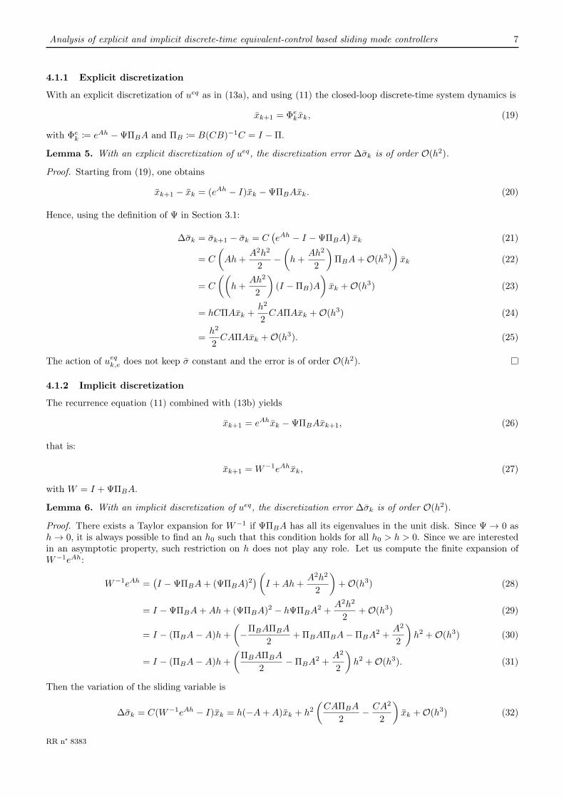
a perturbation ξ(t) = 0.9 sin(t) and α, the magnitude of the discontinuous control, changes. For the present setof simulation, we use α = 1, 3 and 10, values large enough to ensure that the perturbation is always dominatedby the control. On Fig. 10a, we cannot distinguish the three trajectories in the discrete-time sliding phase, sinceeven if usk takes value in a larger set, the selected value within (α, α) does not change. This is supported by theFig. 11a: it is again not possible to differentiate the values taken by the controllers. On the contrary, in Fig. 10b,the three different trajectories are clearly visible. Here we observe that the numerical chattering is dominant. Eachtime we increase α, the amplitudes of the oscillation around the manifold are getting bigger. We also observe thatthe precision of the system seems to be affected by the magnitude of the control. The bigger it is, the farther thesystem oscillates from the origin.

−1.0 −0.8 −0.6 −0.4 −0.2 0.0x1

−0.6−0.4−0.2

0.00.20.40.60.81.0

x2

α = 1

α = 3

α = 10

(a) Implicit discretization of us.

−1.0 −0.8 −0.6 −0.4 −0.2 0.0x1

−0.6−0.4−0.2

0.00.20.40.60.81.0

x2

α = 1

α = 3

α = 10

(b) Explicit discretization of us.

Figure 10: Simulations of system (61) with a perturbation, using different values for α and with h = 0.1s.

8.0 8.5 9.0 9.5 10.0

t

−1.0

−0.5

0.0

0.5

1.0

us(t

)

α = 1

α = 3

α = 10

(a) Implicit discretization of us.

8.0 8.5 9.0 9.5 10.0

t

−10

−5

0

5

10

us(t

)

α = 1

α = 3

α = 10

(b) Explicit discretization of us.

Figure 11: Evolution of us, using different values for α and with h = 0.1 s.

7 Stability properties

7.1 Nominal case

In this subsection, the stability of the system (59) is analyzed. Using the equivalent control proposed in Section 5,the obtained properties can be transposed to the original nominal system (1). Note that the mapping Sgn( · ), asintroduced in Definition 1, has the following properties:

〈v1 − v2, x1 − x2〉 ≥ 0, ∀vi ∈ Sgn(xi), i = 1, 2 (62)0 /∈ Sgn(x), ∀x 6= 0. (63)

Property (62) is known as the monotonicity of the Sgn set-valued function. The positive-definitiveness property ofCB∗ is pivotal to the results presented in this section. Even if it is not explicit with the current notations, CB∗depends on the timestep h. The following lemma gives some insight of when this condition is fulfilled.

Lemma 11. Suppose that CB is positive-definite. There exists an interval I = [0, h∗] ⊂ R+, h∗ > 0 such that ifthe timestep h is chosen in I, then CB∗/h is positive-definite (and so is CB∗ if h 6= 0).

Proof. Let h > 0, CBs and CB∗s are the symmetric part of CB and CB∗, respectively. Let ∆ := CB∗s/h− CBs =∑∞l=1

CAlB+BT (Al)TCT

2(l+1)! hl = O(h). Since CBs is symmetric, it is also normal. Hence we can apply Corollary 4.2.16,

RR n° 8383


p. 405 in [24], which yields that for any eigenvalue µ of CB∗s/h, minλ |λ − µ| ≤ ‖∆‖2,2, with λ an eigenvalue ofCBs and ‖ · ‖2,2 the spectral norm. By definition, ∆ is a symmetric matrix with real entries. Hence ‖∆‖2,2 = δmax,the largest module of any eigenvalue of ∆. Let γ > 0 be the smallest eigenvalue of CBs. If δmax < γ, then everyeigenvalue of CB∗s/h is positive and since CB∗s/h is by definition symmetric, CB∗s/h is positive definite. It is easyto see that ∆ → 0 as h → 0 and that ∆ depends continuously on h. Therefore by Corollary 4.2.4, p. 399 in [24],the eigenvalues of ∆ are continuous functions of h. Then it is always possible to find h∗ such that δmax < γ for allh < h∗, which implies that CB∗s/h is positive-definite and finally CB∗s is positive definite.

Lemma 12. If CB∗ is symmetric positive-definite, then the equilibrium state σ∗ = 0 of (59) is globally Lyapunovstable.

Proof. Let V (σk) := σTk Pσk with P = (CB∗)−1, be a candidate Lyapunov function. Along the trajectories of thesystem (59), one obtains:

V (σk+1)− V (σk) = σTk+1Pσk+1 − σTk Pσk= σTk+1Pσk+1 − (σk+1 − CB∗usk)TP (σk+1 − CB∗usk)

= −(usk)TCB∗usk + 2(usk)T σk+1. (64)

Using (62) with v1 = usk, v2 = 0, x1 = σk+1, and x2 = 0 yields (usk)T σk+1 ≤ 0. Since CB∗ is positive-definite, thefirst term is always nonpositive. This completes the proof.

We can also use a non-quadratic Lyapunov function, inspired by the one presented in [25]. As we shall see, itrelaxes the symmetry condition on the matrix CB∗.

Lemma 13. If CB∗ is positive-definite, then the equilibrium state σ∗ = 0 of (59) is globally Lyapunov stable.

Proof. Let V (σk) := −(usk−1)T σk be the candidate Lyapunov function, and usk−1 ∈ −α Sgn(σk). The function Vis positive definite, radially unbounded, and decrescent since −(usk−1)T σk = α‖σk‖21 and α > 0. Let us study thevariations of V :

V (σk+1)− V (σk) = −(usk)T σk+1 + (usk−1)T σk

= −(usk)T (σk + CB∗usk) + (usk−1)T σk

= −(usk)TCB∗usk + 〈usk−1 − usk, σk〉. (65)

The first term is always nonpositive with the hypothesis on CB∗. For the second term, if usk ∈ −α Sgn(σk+1), thenit also belongs to −α Sgn(0). Hence, by (62), the second term is always nonpositive. This completes the proof.

Proposition 1. If the hypothesis of either Lemma 12 or 13 are satisfied, then the fixed point (σ, u) = (0, 0) of (59)is globally finite-time Lyapunov stable.

Proof. In each case, the difference V (σk+1)− V (σk) consists of −(usk)TCB∗usk plus a nonpositive term. Since CB∗is positive-definite, it holds that −(usk)TCB∗usk ≤ −β‖usk‖2, with β > 0 the smallest eigenvalue of CB∗s . Note thatif σk+1 6= 0, then ‖usk‖ ≥ α and V (σk+1) − V (σk) ≤ −α2β. Iterating, one obtains V (σk+1) − V (σ0) ≤ −kα2β.Let k0 := dV (σ0)/βα2e. Suppose V (σk0+1) 6= 0. Then V (σk0+1) − V (σ0) ≤ −k0α

2β ≤ −V (σ0). This yieldsV (σk0+1) ≤ 0, which implies V (σk0+1) = 0. Then σk0+1 = 0 and σk = 0 for all k > k0.

7.2 Perturbed case

Let us now consider the case with perturbation. The evolution of the sliding variable σ is governed by

σk+1 = σk + CB∗usk + Cpk, (66)

where pk :=∫ tk+1

tkeA(tk+1−τ)Bξ(τ)dτ and usk is the unique solution of the generalized equation (15). Although the

system will never reach and stay on the sliding manifold as in the continuous-time case, it enters the discrete-timesliding phase as stated in Definition 4 and stays in it. Let us first present a technical lemma.

Lemma 14. Let M ∈ Rn×n and Ms := 1/2(M + MT ). Suppose M is positive-definite. Let β > 0 be the smallesteigenvalue of Ms. Then for all x ∈ Rn, ‖M−1x‖ ≤ β−1‖x‖.

Inria


Proof. M−1 exists since Ms is positive-definite. Let νmin (resp. νmax) be the smallest (resp. largest) singularvalues of M (resp. M−1). Two relations hold: νmax = ν−1

min [26, Fact 6.3.21, p.233] and νmin ≥ β > 0 [27,Corollary 3.1.5, p.151]. Then using the spectral norm definition, ‖M−1x‖ ≤ ‖M−1‖‖x‖ = νmax‖x‖ ≤ β−1‖x‖.

From now on, let CB∗s := 1/2(CB∗ + (CB∗)T ) and let β be its smallest eigenvalue.

Proposition 2. Suppose that CB∗ is positive-definite. If α > 0 is such that for all k ∈ N ‖Cpk‖ < αβ, thenthe perturbed closed-loop system (66)-(15) will enter the discrete-time sliding phase in finite time and stay in it.Furthermore if h ∈ [0, h∗], as defined in Lemma 11, then there exists an upper bound T ∗ on the duration of thereaching phase.

Proof. Let V (σk) := −usTk−1σk, usk−1 ∈ −α Sgn(σk). Assume that the system is initialized outside the discrete-

time sliding phase. From Definition 4, it follows that ‖usk‖ ≥ α. Starting from (65), doing as in the proof ofProposition 1 and adding the contribution of the perturbation, we have V (σk+1)− V (σk) ≤ −β‖usk‖2 − (usk)TCpk.Using the Cauchy-Schwarz inequality, we obtain |(usk)TCpk| ≤ ‖usk‖‖Cpk‖. To ensure that V decreases strictly,we need ‖Cpk‖ < β‖usk‖. This condition is satisfied using the hypothesis on the gain α and the fact that β > 0.Note that even in the case with multiple switching surfaces, V decreases as long as the system is not “sliding” onthe intersection of all the manifolds. If σk+1 = 0, then we enter the discrete-time sliding phase. The finite-timeproperty is derived as in the proof of Proposition 1. Let κ = αβ − ‖Cpk‖. From the assumption, κ > 0 holds.In the reaching phase, V decreases by at least κα at each timestep. Hence, V (σk) converges to 0 in finite-time.Now if the system is in the discrete-time sliding phase at tk, then σk+1 = 0 and σk+1 = Cpk. At time tk+1, wehave σk+2 = Cpk + CB∗usk+1. Let us show that usk+1 = −(CB∗)−1Cpk is the unique solution to the generalizedequation (15). With this value, σk+2 = 0. Using Lemma 14 and the hypothesis, ‖usk+1‖ ≤ β−1‖Cpk‖ < α. Relationsbetween norms yield ‖usk+1‖∞ < α. Then usk+1 ∈ (α, α)p ⊂ α Sgn(0) and usk+1 is a solution to (15). With thehypothesis of the proposition, CB∗ is also a P-matrix. Then Lemma 4 can be applied and yields the uniquenessproperty. Thus usk+1 = −(CB∗)−1Cpk is the unique solution to (15) at time tk+1, and by induction, the systemstays in the discrete-time sliding phase.

In the following, we suppose that 0 < h < h∗. Let δ∗max = ‖∆‖2,2 when h = h∗. From the expression ofk0 in the proof of Proposition 1, the duration of the reaching phase is hk0 < V (σ0)h

βα2 + h. Note that β/h is aneigenvalue of CB∗s/h. Applying again Corollary 4.2.16, p. 405 in [24], we have λ − β/h ≤ δmax ≤ δ∗max, with λan eigenvalue of CBs. This yields γ − δ∗max ≤ λ − δ∗max ≤ β/h. Using this in the previous inequality, we gethk0 <

V (σ0)α2(γ−δ∗max) + h∗ =: T ∗.

Remark 2. In continuous time, the condition commonly found is α > ‖ξ‖∞,R+. If the perturbation ξ is continuous,

then it is possible to link this condition to the one used in the previous theorem, ‖Cpk‖ < αβ for all k ∈ N.Using the mean value theorem for integration, we get Cpk = hCeA(tk+1−t′)Bξ(t′) = hCBξ(t′) + O(h2), witht′ ∈ [tk, tk+1]. Hence the first-order estimation for ‖Cpk‖ is h‖CB‖2,2‖ξ‖2 ≤ ‖CB‖2,2

√p‖ξ‖∞. From the proof

of Lemma 11, we have β = hλmin(CB) + O(h2). Then we get α > ‖CB‖2,2√p‖ξ‖∞/β + O(h). Note that

‖CB‖2,2 > λmax(CB) [27, Corollary 3.1.5, p.151]. Therefore ‖CB‖2,2√p‖ξ‖∞/β ≥ 1 and for h small enough,

‖Cpk‖ < αβ implies α > ‖ξ‖∞,R+. If the sliding variable is a scalar, then the converse is also true at the limit.

In the classical literature on discrete-time sliding mode, dealing with the explicit discretization (14a) [1,3,7], twoconditions related to the sliding variable emerged: (σk+1− σk)i(σk)i < 0 for all i = 1, . . . , n, which is necessary; andthe second one is |(σk+1)i| < |(σk)i|. The conditions for linear systems, stated in Lemma 12, 13, and Proposition 2are directly on the system parameters and not on the evolution on the sliding variable, which derives from thedynamics. This fact is, in our sense, much closer to the stability results obtained in continuous-time [25].

Let us now turn our attention to the relationship between u and u. In particular, we study the convergence ofu to u during the discrete-time sliding phase, which is established after T ∗ < +∞.

Proposition 3. Consider the discrete-time closed-loop system given by (66) and (15). Let {hn}n∈N be any strictlydecreasing sequence of positive numbers converging to 0 and with h0 < h∗ (see Lemma 11). Suppose that theperturbation ξ : R→ Rp is uniformly continuous, that CB is positive-definite and that α > 0 is chosen such that theconditions of Proposition 2 are satisfied for each timestep hn. Then for any S ⊆ [T ∗,∞), limhn→0‖us−us‖∞,S = 0.

Proof. Let {tk} be a sequence such that for all k ∈ N, tk+1 − tk = hn. For the sake of clarity, we omit towrite explicitly the dependence on n. From Proposition 2 and Lemma 11, we know that for all k such thattk ≥ T ∗, usk = −(CB∗)−1Cpk−1 = −(CB∗)−1C

∫ tktk−1

eA(tk−τ)Bξ(τ)dτ . During the sliding phase, the continuous-time controller satisfies us(t) = −ξ(t). Let S be any time interval contained in [T ∗,+∞). Let t ∈ S and k ∈ N is

RR n° 8383


such that t ∈ [tk, tk+1). Hence us(t) = usk. Let us study usk − us(t):

usk − us(t) = −(CB∗)−1C

∫ tk

tk−1

eA(tk−τ)Bξ(τ)dτ + ξ(t) (67)

= −(CB∗)−1

(∫ tk

tk−1

CeA(tk−τ)Bξ(τ)dτ − CB∗ξ(t)

). (68)

Using (12), we obtain:

usk − us(t) = −(CB∗)−1

(∫ tk

tk−1

CeA(tk−τ)Bξ(τ)dτ −∫ tk+1

tk

CeA(tk+1−τ)Bξ(t)dτ

). (69)

With the change of variable τ ′ = τ + hn in the first integral, we can group the two integrals in (69) as follows:

usk − us(t) = −(CB∗)−1

(∫ tk+1

tk

CeA(tk+1−τ)B(ξ(τ − hn)− ξ(t)dτ)

(70)

= −(CB∗)−1

(∫ tk+1

tk

CB(ξ(τ − hn)− ξ(t)) +

∞∑l=1

CAlB

l!

((tk+1 − τ)l(ξ(τ − hn)− ξ(t))

)dτ

). (71)

Using again (12), let us provide an approximation for the first factor:

(CB∗)−1 =

(hnCB +

∞∑l=1

CAlB

(l + 1)!hl+1n

)−1

(72)

=

(I +

∞∑l=1

(CB)−1CAlB

(l + 1)!hln

)−1

(hnCB)−1 (73)

=

(I − (CB)−1CAB

2hn +O(h2

n)

)(hnCB)−1. (74)

The Taylor expansion holds if∑∞l=1

(CB)−1CAlB(l+1)! hln has all its eigenvalues in the unit disk. This is a mere technical

restriction, since it is always possible to find a small enough positive number hn0 such this condition is satisfied.Since we are interested in the case where {hn} converges to 0, this requirement is supposed to hold. For the firstterm in the integrand in (71), we apply the mean value theorem for integration. If ξ is a vector-valued function(this is the case when the sliding variable has dimension greater than 1), we apply the theorem for each componentseparately. This yields for i = 1, . . . , n (

∫ tk+1

tkξ(τ − hn)− ξ(t)dτ)i = hn(ξi(t

′i− hn)− ξi(t)) for some t′i ∈ [tk, tk+1].

For the second part of the integrand in (71), we exchange the summation and integral signs. This is possible sincethe matrix exponential converges normally and ξ is bounded on any interval [tk, tk+1] (ξ is continuous). Moreover forall l ≥ 1, with τ ∈ [tk, tk+1], (tk+1−τ)lξ(τ−hn)−ξ(t)) = O(hn). Thus

∫ tk+1

tk(tk+1−τ)l(ξ(τ−hn)−ξ(t))dτ = O(h2

n).Then (71) can be rewritten as:

usk − us(t) = −(I +O(hn))

(∫ tk+1

tk

h−1n (ξ(τ − hn)− ξ(t))dτ +O(hn)

). (75)

Taking the supremum norm yields:

‖usk − us(t)‖∞ ≤ ‖I +O(hn))‖∞

(maxi

supt∈[tk,tk+1]

|ξi(t′i − h)− ξi(t)|+ ‖O(hn)‖∞

)(76)

≤ maxi

supt∈[tk,tk+1]

|ξi(t′i − hn)− ξi(t)|+O(hn). (77)

Since ξ is uniformly continuous, for every ε > 0, there exists δ > 0 such that for all t1, t2 ∈ R, |t1 − t2| ≤ δ implies‖ξ(t1)− ξ(t2)‖ ≤ ε. Then the right-hand side of (77) is converging to 0 as hn → 0. Since this is true for all t ∈ S,the proof is complete.

Inria


It is also interesting to study the convergence of the variation of the control variable, which may be thought ofas a measure of the control input chattering. Let us first define the variation of a function in some special cases.The material in Definitions 5 and 6 is adapted from [28].

Definition 5. Let f : R→ Rm be a right-continuous step function, discontinuous at finitely many time instants tkand t0, T ∈ R, t0 < T . Then the variation of f on [t0, T ] is defined as:

VarTt0(f) :=∑k

‖f(tk)− f(tk−1)‖, (78)

with k ∈ N such that tk ∈ (t0, T ].

Definition 6. Let f : R→ Rm be a continuously differentiable function, with bounded derivatives and let t0, T ∈ R,t0 < T . Then the variation of f on [t0, T ] is defined as:

VarTt0(f) :=

∫ T

t0

‖f(τ)‖dτ. (79)

Proposition 4. Let {hn}n∈N be any strictly decreasing sequence of positive numbers converging to 0 with h0 < h∗.Suppose that CB is positive-definite, and ξ is a real-valued continuously differentiable with bounded derivativefunction. Let α be chosen such that the conditions of Proposition 2 are verified for each hn. Then lim

hn→0VarTT∗(u

s) =

VarTT∗(us).

Proof. Let {tk} be a sequence such that for all k ∈ N, tk+1− tk = hn. Let us recall that, with the implicit controllerdefined in Equations (66) and (15), the reaching phase duration is bounded and that the sliding phase is establishedat t = T ∗ if h is small enough. Let VarTT∗(u

s) denote the variation of the function us on the time interval [T ∗, T ].The variation of the step function us is:

VarTt0(us) =∑k

‖usk+1 − usk‖ =∑k

‖(CB∗)−1C

∫ tk+1

tk

eA(tk+1−τ)Bξ(τ)dτ − (CB∗)−1C

∫ tk

tk−1

eA(tk−τ)Bξ(τ)dτ‖ (80)

=∑k

‖(CB∗)−1

(∫ tk+1

tk

CB(ξ(τ)− ξ(τ − hn))dτ +

∫ tk+1

tk

C(eA(tk+1−τ) − I)B(ξ(τ)− ξ(τ − hn))

)‖. (81)

Using the approximation for (CB∗)−1 obtained in (74), we get:

VarTt0(us) ≤ (I +O(hn))∑k

‖∫ tk+1

tk

ξ(τ)− ξ(τ − hn)

hndτ‖ (82)

+ (I +O(hn))∑k

‖(CB)−1

∫ tk+1

tk

C(eA(tk+1−τ) − I)Bξ(τ)− ξ(τ − hn)

hndτ‖ (83)

≤ (I +O(hn))

∫ T

t0

‖ξ(τ)− ξ(τ − hn)

hn‖dτ (84)

+ (I +O(hn))∑k

‖(CB)−1

∫ tk+1

tk


hndτ‖. (85)

Using standard estimation inequalities, we obtain the following estimation for all integrals in the sum:

‖∫ tk+1

tk


hndτ‖ ≤

∫ tk+1

tk

‖C‖‖B‖(e‖A‖hn − 1)‖ξ(τ)− ξ(τ − hn)

hn‖dτ. (86)

Then we can group the terms in (85) as:

VarTt0(us) ≤ (I +O(hn))

∫ T

t0

‖ξ(τ)− ξ(τ − hn)

hn‖dτ

+ (I +O(hn))‖(CB)−1‖∫ T

t0

‖C‖‖B‖(e‖A‖hn − 1)‖ξ(τ)− ξ(τ − hn)

hn‖dτ. (87)

Since ξ is continuously differentiable,∫ Tt0‖ ξ(τ)−ξ(τ−hn)

hn‖dτ converges to

∫ Tt0‖ξ(τ)‖dτ = VarTt0(us) as hn → 0. All the

other terms in the right-hand side of (87) converge to 0 as hn → 0.

RR n° 8383


7.3 Comparison with saturated SMC

0.0 0.2 0.4 0.6 0.8 1.0

saturation parameter ε

0.00

0.02

0.04

0.06

0.08

0.10

tim

e s

tep h

0.02 0.06 0.10 0.14 0.18

performance index

1 2

3

(a) Simulation results with 100 regularly spaced values forthe timestep h and 100 logarithmically spaced values for thesaturation parameter ε.

0.02 0.04 0.06 0.08 0.10


0.00

0.02

0.04

0.06

0.08

0.10

tim

e s

tep h

-0.030-0.0

20-0

.010

0.01

00.

0200.

030

best (ε,h) for all timestep

0.02 0.06 0.10 0.14 0.18

performance index

0.00

0

1 2 3

(b) Detail of Fig. 12a, 300 values for h and 1000 values for ε,forming a regular grid. Level sets were also added to showthe difference in performance between the implicit discretiza-tion and the explicit one with saturation. If the difference ispositive, the explicit saturated control is performing betterthan the implicit one.

Figure 12: Simulation results of a perturbed system controlled using sliding mode with a saturation. The perfor-mance index is the sum of the |σk| for the last 20s.

We simulate the system (61) with a perturbation ξ(t) = sin 4πt. Instead of using a discontinuous control, we

use the following input: us(t) = − satε(σ(t)) with satε(x) =

{x/ε if |x| ≤ εsgn(x) if |x| > ε

. As in Section 6, each simulation

lasts 150s. We use two metrics to measure the performance of the different controllers. To measure the (output)chattering, due to the discretization and the perturbation, we sum the absolute value of the sliding variable σk forthe last 20s: C1 :=

∑k |σk|. To measure the control effort (or input chattering), we measure the variation of the

control for the last 20s: C2 := VarTT−20(us). Each quantity defines the performance index in Fig. 12 or 13. Wechoose to consider only the last 20s of each simulation to capture the behaviour near the sliding manifold. Letus recall that without perturbation, the implicit controller always supersedes the saturated explicit one, since itsuppresses numerical chattering and usk = 0 in the discrete-time sliding phase. With both index, we can divide thespace into 3 cones, numbered 1, 2 and 3 in Fig. 12 and 13. This separation helps us to compare both controllers. InFig. 12a the performance in term of chattering is presented. For large values of ε, the chattering does not changewhen the timestep varies: the control action does not attenuate the effect of the perturbation. With a small ε, thebehaviour is richer, as depicted in Fig.12b. On Fig. 12b, the overall best performance is obtained with small valuesfor both ε and h. However for small values of ε, the performance can degrade rapidly if the sampling period h isnot small enough, as seen in region 1. The dark points indicate for each value of h the pair (ε, h) of parametersyielding the best performance. It seems that there is a linear relationship between those values. However it isunclear if this observation on one particular system remains valid with a different perturbation. The level sets inFig. 12b are used to compare the performance of the implicit and the saturated explicit controllers. On Fig. 13, theperformance in terms of control cost is presented. The best performance is achieved for large ε since the slope ofthe saturated function is gentle. On the other hand in Fig. 13b, with a small ε, the cost increases and explodes withε close to 0, as in region 1. The level sets indicate the difference between the costs of the 2 different controllers. Itis worth noting that on region 2 where the saturated controller is better in Fig. 12b, it has a higher cost in term ofcontrol (Fig. 13b). In region 3, where the saturated controller performs less in terms of chattering (Fig. 12a), it hasa smaller cost in terms of control (Fig. 13a). Indeed with a large ε, the control input is small when the closed-loop

Inria


0.0 0.2 0.4 0.6 0.8 1.0


0.00

0.02

0.04

0.06

0.08

0.10

tim

est

ep h

102 103 104

performance index

12

3

(a) Simulation results with 100 regularly spaced values forthe timestep h and 100 logarithmically spaced values for thesaturation parameter ε.

0.02 0.04 0.06 0.08 0.10


0.00

0.02

0.04

0.06

0.08

0.10

tim

est

ep h

50.0

00

15.0

00

0.00

0

-300.0

00

-15.

000

-15.000

102 103 104

performance index

1

2

3

(b) Detail of Fig. 13a, 300 values for h and 1000 values for ε,forming a regular grid. Level sets were also added to showthe difference in performance between the implicit discretiza-tion and the explicit one with saturation. If the difference ispositive, the explicit saturated control is performing betterthan the implicit one.

Figure 13: Simulation results of the same perturbed system controlled using sliding mode with a saturation. Theperformance index is the sum of the |usk+1 − usk| for the last 20s.

system is close to the sliding manifold. The cost is then very small, but the disturbance is not attenuated at all.The implicit controller appeals to us as the best compromise between the input and output chattering. It is alsovery easy to use, since it requires no particular tuning with respect to the timestep or the perturbation.

8 Conclusion

In this article several time discretizations of the classical ECB-SMC method are analysed, from the point of viewof their ability to alleviate or suppress the numerical chattering, and to guarantee the finite-time reachability of thesliding surface. A new discrete-time sliding mode control scheme is also proposed. The analysis is led from analyticalestimations, as well as numerical simulations obtained with the INRIA software package siconos. In particular theinfluence of the discretization method of the state-continuous equivalent controller is studied, as well as the one ofthe discontinuous part of the input (explicit versus implicit discretizations). The nominal and perturbed cases areconsidered. The simulation results indicate that the use of an explicit discretization for the discontinuous part ofthe input yields numerical chattering. This is not the case when using an implicit discretization. We also providean example where the use of an explicit discretization of ueq makes the closed-loop system diverge, whereas withthe other methods it attains the sliding surface. The issues related to the Lyapunov stability of the discrete-timesliding variable are also studied, using the monotonicity properties of the underlying discontinuous (set-valued)controller. Further works will include conducting experimental studies and also improvements in the perturbationattenuation.

Bibliography

References

[1] S. Sarpturk, Y. Istefanopulos, and O. Kaynak, “On the stability of discrete-time sliding mode control systems,”Automatic Control, IEEE Transactions on, vol. 32, no. 10, pp. 930–932, 1987.

RR n° 8383


[2] S. Drakunov and V. Utkin, “On discrete-time sliding modes,” in Proc. of IFAC Nonlinear Control SystemDesign Conf., 1989, pp. 273–278.

[3] K. Furuta, “Sliding mode control of a discrete system,” Systems & Control Letters, vol. 14, no. 2, pp. 145–152,1990.

[4] V. Utkin, “Sliding mode control in discrete-time and difference systems,” in Variable Structure and LyapunovControl, ser. Lecture Notes in Control and Information Sciences. Springer, 1994, vol. 193, pp. 87–107.

[5] W. Gao, Y. Wang, and A. Homaifa, “Discrete-time variable structure control systems,” Industrial Electronics,IEEE Transactions on, vol. 42, no. 2, pp. 117–122, 1995.

[6] G. Golo and C. Milosavljević, “Robust discrete-time chattering free sliding mode control,” Systems & ControlLetters, vol. 41, no. 1, pp. 19–28, 2000.

[7] C. Milosavljević, “General conditions for the existence of a quasi-sliding mode on the switching hyperplane indiscrete variable structure systems,” Automation and Remote Control, vol. 46, no. 3, pp. 307–314, 1985.

[8] Z. Galias and X. Yu, “Complex discretization behaviors of a simple sliding-mode control system,” Circuits andSystems II: Express Briefs, IEEE Transactions on, vol. 53, no. 8, pp. 652–656, 2006.

[9] ——, “Analysis of zero-order holder discretization of two-dimensional sliding-mode control systems,” Circuitsand Systems II: Express Briefs, IEEE Transactions on, vol. 55, no. 12, pp. 1269–1273, 2008.

[10] B. Wang, X. Yu, and G. Chen, “ZOH discretization effect on single-input sliding mode control systems withmatched uncertainties,” Automatica, vol. 45, no. 1, pp. 118–125, 2009.

[11] V. Acary and B. Brogliato, “Implicit Euler numerical scheme and chattering-free implementation of slidingmode systems,” Systems & Control Letters, vol. 59, no. 5, pp. 284–293, 2010.

[12] V. Acary, B. Brogliato, and Y. Orlov, “Chattering-free digital sliding-mode control with state observer anddisturbance rejection,” Automatic Control, IEEE Transactions on, vol. 57, no. 5, pp. 1087–1101, 2012.

[13] F. Plestan, V. Bregeault, A. Glumineau, Y. Shtessel, and E. Moulay, “Advances in high order and adaptivesliding mode control–theory and applications,” in Sliding Modes after the First Decade of the 21st Century,ser. Lecture Notes in Control and Information Sciences. Springer, 2012, vol. 412, pp. 465–492.

[14] M. Defoort, T. Floquet, A. Kokosy, and W. Perruquetti, “A novel higher order sliding mode control scheme,”Systems & Control Letters, vol. 58, no. 2, pp. 102–108, 2009.

[15] R. Cottle, J.-S. Pang, and R. Stone, The Linear Complementarity Problem, ser. Classics in Applied Mathe-matics. Society for Industrial Mathematics, 2009, no. 60.

[16] C. Edwards and S. Spurgeon, Sliding Mode Control: Theory and Applications, ser. Systems and Control BookSeries. CRC Press, 1998, vol. 7.

[17] B. Wang, X. Yu, and X. Li, “ZOH discretization effect on higher-order sliding-mode control systems,” IndustrialElectronics, IEEE Transactions on, vol. 55, no. 11, pp. 4055–4064, 2008.

[18] F. Facchinei and J.-S. Pang, Finite-Dimensional Variational Inequalities and Complementarity Problems, ser.Springer Series in Operations Research. Springer, 2003.

[19] V. Acary and B. Brogliato, Numerical Methods for Nonsmooth Dynamical Systems: Applications in Mechanicsand Electronics, ser. Lecture Notes in Applied and Computational Mechanics. Springer Berlin Heidelberg,2008, vol. 35.

[20] K. Furuta and Y. Pan, “Discrete-time variable structure control,” in Variable Structure Systems: Towards the21st Century, ser. Lecture Notes in Control and Information Sciences, J.-X. Yu X., Xu, Ed. Springer BerlinHeidelberg, 2002, vol. 472, pp. 57–81.

[21] C.-F. Lin and W.-C. Su, “A total chattering-free sliding mode control for sampled-data systems,” in AmericanControl Conference, 2004. Proceedings of the 2004, vol. 3. IEEE, 2004, pp. 1940–1945.

Inria


[22] V. Acary and F. Pérignon, “An introduction to Siconos,” INRIA, Rapport Technique RT-0340, 2007.[Online]. Available: http://hal.inria.fr/inria-00162911

[23] J. D. Hunter, “Matplotlib: a 2D graphics environment,” Computing in Science & Engineering, pp. 90–95, 2007.

[24] D. Hinrichsen and A. J. Pritchard, Mathematical Systems Theory I, ser. Texts in Applied Mathematics.Springer Berlin Heidelberg, 2005, vol. 48.

[25] V. Utkin, Sliding Modes in Control and Optimization, ser. Communications and Control Engineering. SpringerBerlin, 1992.

[26] D. Bernstein, Matrix Mathematics. Princeton University Press Princeton, NJ, 2005.

[27] R. A. Horn and C. R. Johnson, Topics in Matrix Analysis. Cambridge University Press, 1994.

[28] L. Ambrosio, N. Fusco, and D. Pallara, Functions of Bounded Variation and Free Discontinuity Problems.Clarendon Press Oxford, 2000.

RR n° 8383

http://hal.inria.fr/inria-00162911

RESEARCH CENTREGRENOBLE – RHÔNE-ALPES

Inovallée655 avenue de l’Europe Montbonnot38334 Saint Ismier Cedex

PublisherInriaDomaine de Voluceau - RocquencourtBP 105 - 78153 Le Chesnay Cedexinria.fr

ISSN 0249-6399

Documents

Analysis of explicit and implicit discrete-time equivalent