IJCSIET-ISSUE5-VOLUME3-SERIES2 Page 1

IJCSIET--International Journal of Computer Science inf ormation and Engg., Technologies ISSN 2277-4408 || 01102015-022

Analysis of Flow distribution in 3D high speed turbine.

Vinod M,G.leela Siva Ram Prasad – M.Tech

DJR College of Engineering & Technology

Email -vinodmummina@gmail.xom

ABSTRACT

The project Deals with the Computational

Flu id Dynamic analysis of Flow through High

speed turbine. The turbine is main ly used in the

power generation process at first the model is

designed in the commercial software package solid

works and analyzed in the Fluent. The main aim of

the project is to derive the Temperature and other

physical parameters of the turbine in this project we

firstly use water as a fluid and we extract the

readings from the Fluent and after we analyses the

turbine with air and analyses the turbine for one

more t ime and we compare the results of physical

parameters. The whole work involves numerous

computational facilities and skills.

INTRODUCTION

A water turbine is arotary engine that

converts kinetic and potential energy of water

into mechanical work. Water turbines were

developed in the 19th century and were widely

used for industrial power prior to electrical grids.

Now they are mostly used for electric

power generation. Water turbines are mostly found

in dams to generate electric power from

water kinetic energy.

Types of Water Turbines

Water turbines are divided into two

groups; reaction turbines and impulse turbines.

The precise shape of water turbine b lades is a

function of the supply pressure of water, and the

type of impeller selected.

REACTION TURBINES

Reaction turbines are acted on by water,

which changes pressure as it moves through the

turbine and gives up its energy. They must be

encased to contain the water pressure (or suction),

or they must be fully submerged in the water flow.

Newton's third law describes the transfer of energy

for react ion turbines. Most water turbines in use are

reaction turbines and are used in low (<30 m or

100 ft) and medium (30–300 m or 100–1,000 ft)

head applications. In reaction turbine pressure drop

occurs in both fixed and moving blades. It is

largely used in dam and large power p lants

REACTION TURBINES :

VLH turbine

Francis turbine

Kaplan turbine

Tyson turbine

Gorlov helical turbine

Francis Turbine

Francis turbine, a type of widely used

water turbine. Francis turbine is one having a

runner with buckets, usually nine or more to which

the water enters the turbine in a radial direction

with respect to shaft. The Francis turbine is a type

of water turbine that was developed by James B.

IJCSIET-ISSUE5-VOLUME3-SERIES2 Page 2

IJCSIET--International Journal of Computer Science inf ormation and Engg., Technologies ISSN 2277-4408 || 01102015-022

Francis in Lowell, Massachusetts. It is an inward-

flow react ion turbine that combines radial and axial

flow concepts. Francis turbines are the most

common water turbine in use today. They operate

in a water head from 40 to 600 m (130 to 2,000 ft)

and are primarily used for electrical power

production. The electric generator which most

often use this type of turbine, have a power output

which generally ranges just a few kilowatts up to

800 MW, though mini-hydro installat ions may be

lower. Penstock (input pipes) diameters are

between 3 and 33 feet (0.91 and 10.06 meters). The

speed range of the turbine is from 83 to 1000 rpm.

Wicket gates around the outside of the turbine's

rotating runner control the rate of water flow

through the turbine for different power production

rates. Francis turbines are almost always mounted

with the shaft vertical to keep water away from the

attached generator and to facilitate installation and

maintenance access to it and the turbine.

IMPULS E TURBINES

Impulse turbines change the velocity of a

water jet. The jet pushes on the turbine's curved

blades which changes the direction of the flow. The

resulting change in momentum (impulse) causes a

force on the turbine blades. Since the turbine is

spinning, the force acts through a distance (work)

and the diverted water flow is left with dimin ished

energy. An impulse turbine is one which the

pressure of the fluid flowing over the rotor blades

is constant and all the work output is due to the

change in kinetic energy of the fluid. Prior to

hitting the turbine blades, the water's pressure

(potential energy) is converted to kinetic energy by

a nozzle and focused on the turbine. No pressure

change occurs at the turbine blades, and the turbine

doesn't require housing for operation. Newton's

second law describes the transfer of energy for

impulse turbines. Impulse turbines are often used

in very high (>300m/1000 ft) head applications.

IMPULS E TURBINE

Water wheel

Pelton wheel

Turgo turbine

Cross-flow turbine (also known as the

Bánki-Michell turbine, or Ossberger turbine)

Jonval turbine

Reverse overshot water-wheel

Screw turbine

Barkh Turb ine

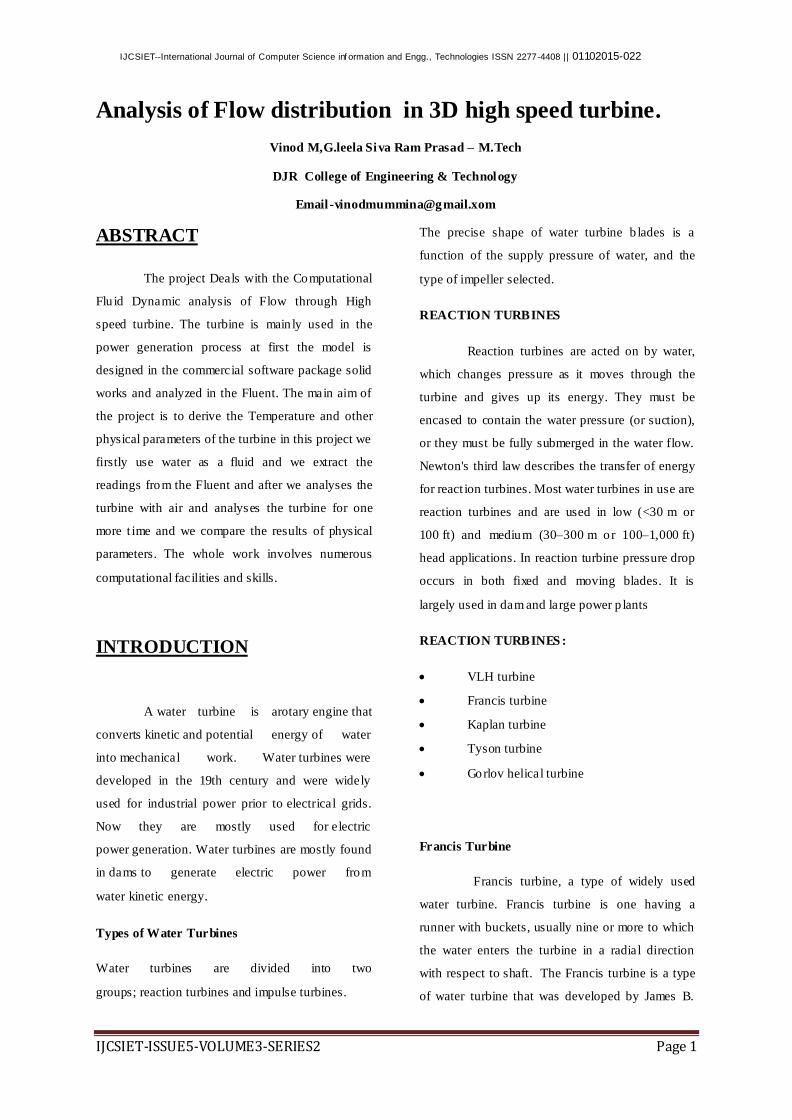
Design and Application

Figure1. Ture Application chart

Turbine selection is based on the available

water head, and less so on the available flow rate.

In general, impulse turbines are used for high head

sites, and reaction turbines are used for low

head sites. Kaplan turbines with adjustable blade

pitch are well-adapted to wide ranges of flow or

head conditions, since their peak efficiency can be

achieved over a wide range of flow conditions.

Small turbines (mostly under 10 MW) may have

horizontal shafts, and even fairly large bulb-type

turbines up to 100 MW or so may be horizontal.

Very large Francis and Kaplan machines usually

IJCSIET-ISSUE5-VOLUME3-SERIES2 Page 3

IJCSIET--International Journal of Computer Science inf ormation and Engg., Technologies ISSN 2277-4408 || 01102015-022

have vertical shafts because this makes best use of

the available head, and makes installation of a

generator more economical. Pelton wheels may be

either vertical or horizontal shaft machines because

the size of the machine is so much less than the

available head. Some impulse turbines use multiple

jets per runner to balance shaft thrust. This also

allows for the use of a s maller turbine runner,

which can decrease costs and mechanical losses.

Typical Range Of Heads

• Water wheel 0.2 < H < 4 (H = head

in m)

• Screw turbine 1 < H < 10

• VLH turbine 1.5 < H < 4.5

• Kaplan turbine 20 < H < 40

• Francis turbine 40 < H < 600

• Pelton wheel 50 < H < 1300

• Turgo turbine 50 < H < 250

High Speed turbine

The High Speed turbine is a type of water

turbine that was developed in Lowell,

Massachusetts. It is an inward-flow reaction

turbine that combines radial and axial flow

concepts. High Speed turbines are the most

common water turb ine in use today. They operate

in a water head from 40 to 600 m (130 to 2,000 ft)

and are primarily used for electrical power

production. The electric generators which most

often use this type of turbine have a power output

which generally ranges just a few kilowatts up to

800 MW, though min i-hydro installations may be

lower. Penstock (input pipes) diameters are

between 3 and 33 feet (0.91 and 10.06 meters). The

speed range of the turbine is from 75 to 1000 rpm.

Wicket gates around the outside of the turbine's

rotating runner control the rate of water flow

through the turbine for different power production

rates. High Speed turbines are almost always

mounted with the shaft vertical to isolate water

from the generator. This also facilitates installation

and maintenance.

The water flow in the High Speed turbine

must be in the form of radial direction and exists

through the turbine axially. When the turbine

impart ing then the water pressure must be

decreases and is hits the blades when turbine

rotates. It is the first turbine with a radial inflow. It

is also known as reaction turbine. Compare to the

impulse turbine has some features. We can see the

major p ressure drop in the turbine. Up to the entry

point we can see the complete pressure drop in the

impulsive turbine. During the operation in the

water flow is completely.

Design of high speed turbine

High Speed turbine consists of circular

plates which are fixed to the rotating shafts and is

perpendicular to the surface. The water flow takes

from the centre. We can notice the curved channels

on the circular p lates. The plate with the channels is

known as runner. The runner is surrounding by a

ring of mot ionless channels which is known as

guide vanes. With the help of the spiral casing the

guide vanes are mounted which is known as volute.

We can see the exit of the flow from the centre of

the runner plate. To the central exit of the runner

the draft tube is attached. During the time of

designing we can also notice the design parameter

like angles of vanes, radius of the runner, curvature

of channel, size of the turbine must be depends

upon the size of the head availab le.

Working of High S peed Turbine

High Speed turbines are the most

preferred hydraulic turbines. They are the most

reliable workhorse of hydroelectric power

stations. It contributes about 60 percentage of

the global hydropower capacity, main ly

because it can work efficiently under a wide

range of operating conditions. Water head and

IJCSIET-ISSUE5-VOLUME3-SERIES2 Page 4

IJCSIET--International Journal of Computer Science inf ormation and Engg., Technologies ISSN 2277-4408 || 01102015-022

flow rate are the most vital input parameters

that govern performance of a hydraulic turbine.

But these parameters are subjected to seasonal

variation in a hydroelectric power station.

High Speed turbine is capable of delivering

high efficiency even if there is a huge variation

in these flow parameters. The preferable Head

and Flow ranges for High Speed turbine is 45-

400 m and 10-700 m3/s

In this article we will understand working

of High Speed turbine and will also realize why it

is capable to work under varying flow condit ions.

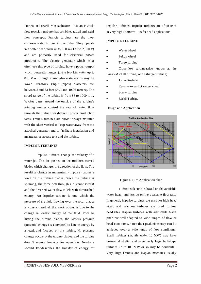
Most important part of High Speed turbine is its

runner. It is fitted with a collection of complex

shaped blades as shown in Fig.1

Figure2.So lid Works Designed Model

Figure3.Actual Model

In runner water enters radially, and leaves axially.

During the course of flow, water glides over

runner blades as shown in figure below.

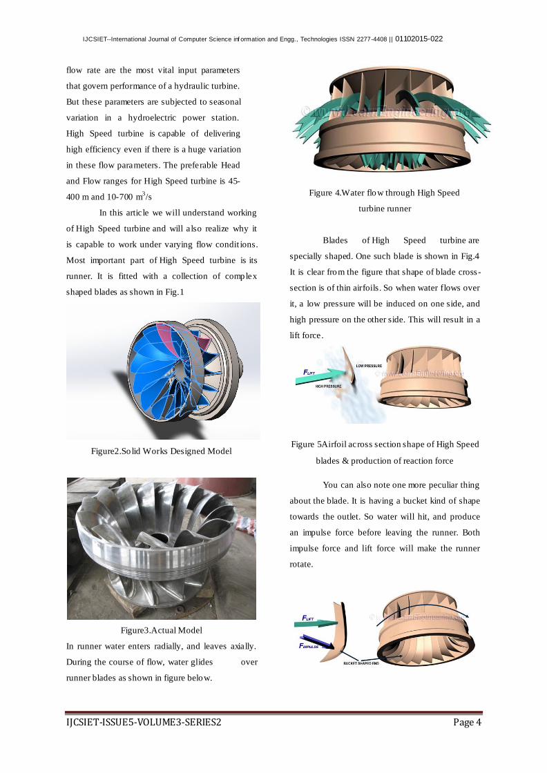
Figure 4.Water flow through High Speed

turbine runner

Blades of High Speed turbine are

specially shaped. One such blade is shown in Fig.4

It is clear from the figure that shape of blade cross-

section is of thin airfoils. So when water flows over

it, a low pressure will be induced on one side, and

high pressure on the other side. This will result in a

lift force.

Figure 5Airfoil across section shape of High Speed

blades & production of reaction force

You can also note one more peculiar thing

about the blade. It is having a bucket kind of shape

towards the outlet. So water will hit, and produce

an impulse force before leaving the runner. Both

impulse force and lift force will make the runner

rotate.

IJCSIET-ISSUE5-VOLUME3-SERIES2 Page 5

IJCSIET--International Journal of Computer Science inf ormation and Engg., Technologies ISSN 2277-4408 || 01102015-022

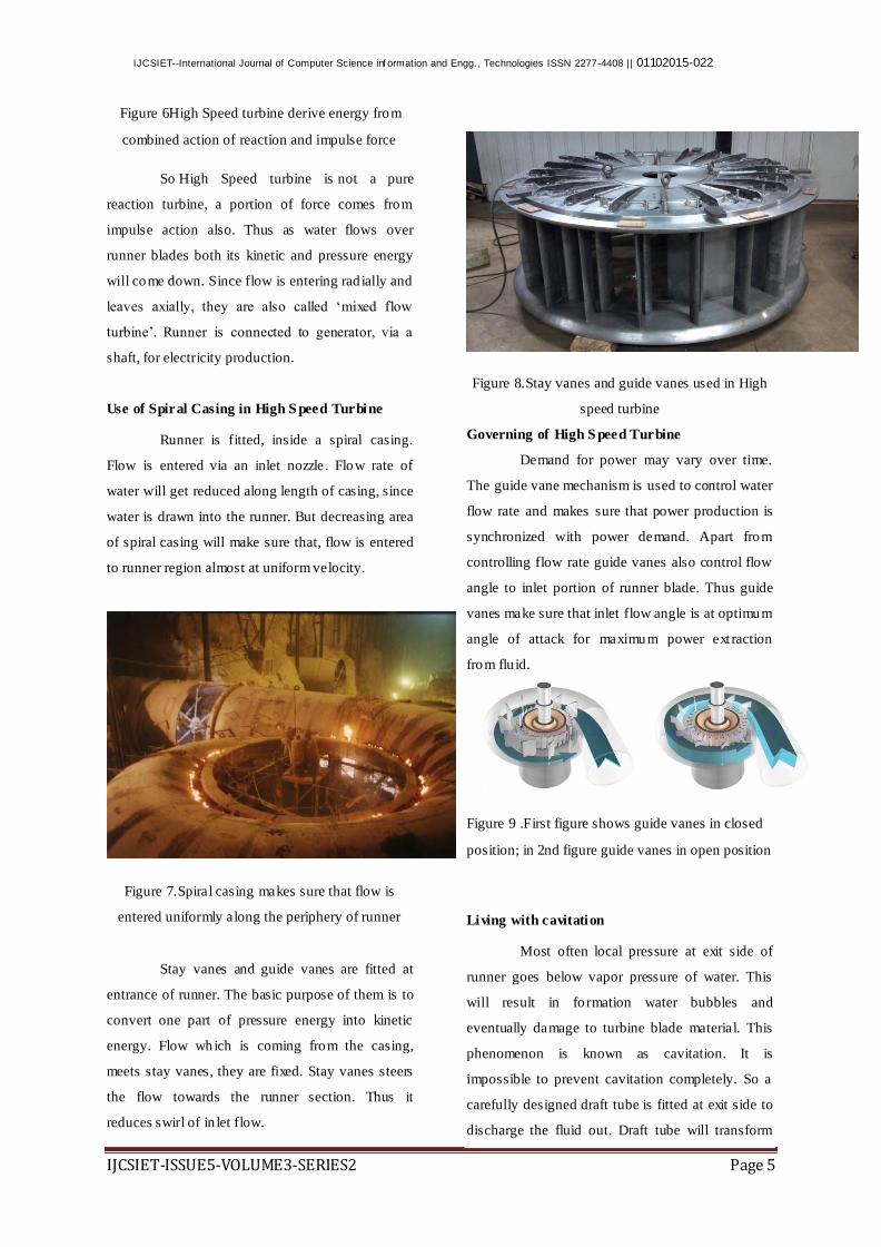
Figure 6High Speed turbine derive energy from

combined action of reaction and impulse force

So High Speed turbine is not a pure

reaction turbine, a portion of force comes from

impulse action also. Thus as water flows over

runner blades both its kinetic and pressure energy

will come down. Since flow is entering rad ially and

leaves axially, they are also called „mixed flow

turbine‟. Runner is connected to generator, via a

shaft, for electricity production.

Use of Spiral Casing in High S peed Turbine

Runner is fitted, inside a spiral casing.

Flow is entered via an inlet nozzle. Flow rate of

water will get reduced along length of casing, since

water is drawn into the runner. But decreasing area

of spiral casing will make sure that, flow is entered

to runner region almost at uniform velocity.

Figure 7.Spiral casing makes sure that flow is

entered uniformly along the periphery of runner

Stay vanes and guide vanes are fitted at

entrance of runner. The basic purpose of them is to

convert one part of pressure energy into kinetic

energy. Flow which is coming from the casing,

meets stay vanes, they are fixed. Stay vanes steers

the flow towards the runner section. Thus it

reduces swirl of in let flow.

Figure 8.Stay vanes and guide vanes used in High

speed turbine

Governing of High S peed Turbine

Demand for power may vary over time.

The guide vane mechanism is used to control water

flow rate and makes sure that power production is

synchronized with power demand. Apart from

controlling flow rate guide vanes also control flow

angle to inlet portion of runner blade. Thus guide

vanes make sure that inlet flow angle is at optimum

angle of attack for maximum power ext raction

from flu id.

Figure 9 .First figure shows guide vanes in closed

position; in 2nd figure guide vanes in open position

Living with cavitation

Most often local pressure at exit side of

runner goes below vapor pressure of water. This

will result in fo rmation water bubbles and

eventually damage to turbine blade material. This

phenomenon is known as cavitation. It is

impossible to prevent cavitation completely. So a

carefully designed draft tube is fitted at exit side to

discharge the fluid out. Draft tube will transform

IJCSIET-ISSUE5-VOLUME3-SERIES2 Page 6

IJCSIET--International Journal of Computer Science inf ormation and Engg., Technologies ISSN 2277-4408 || 01102015-022

velocity head to static head due to its increasing

area and will reduce effect of cavitation. As we can

observe the increase in area from top to bottom in

the Draft tube.

Figure 10.Conversion of velocity head to static

head with help of draft tube.

Geometric Modeling Of High

Speed Turbine In Solid Works

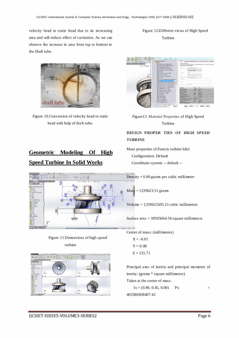
Figure 11.Dimensions of high speed

turbine

Figure 12.Different views of High Speed

Turbine

Figure13 .Material Properties of High Speed

Turbine

DES IGN PROPER TIES OF HIGH SPEED

TURBINE

Mass properties of Francis turbine bilal

Configuration: Default

Coordinate system: -- default --

Density = 0.00 grams per cubic millimeter

Mass = 1239623.51 grams

Volume = 1239623505.21 cubic millimeters

Surface area = 30595664.56 square millimeters

Center of mass: (millimeters)

X = -0.01

Y = 0.08

Z = 215.71

Principal axes of inert ia and principal moments of

inertia: (grams * square millimeters)

Taken at the center of mass.

Ix = (0.89, 0.45, 0.00) Px =

403580458407.42

IJCSIET-ISSUE5-VOLUME3-SERIES2 Page 7

IJCSIET--International Journal of Computer Science inf ormation and Engg., Technologies ISSN 2277-4408 || 01102015-022

Iy = (-0.45, 0.89, 0.00) Py =

403692095937.14

Iz = (0.00, -0.00, 1.00) Pz =

551952787695.30

Moments of inertia: (grams * square millimeters)

Taken at the center of mass and aligned with the

output coordinate system.

Lxx = 403602855509.35 Lxy = 44707585.02 Lxz = -7122681.51

Lyx = 44707585.02 Lyy =

403669700670.54 Lyz = 14878641.21

Lzx = -7122681.51 Lzy = 14878641.21 Lzz = 551952785859.98

Moments of inertia: (grams * square millimeters)

Taken at the output coordinate system.

Ixx = 461282997565.11 Ixy = 44706667.96 Ixz = -9650510.70

Iyx = 44706667.96 Iyy =

461349835245.71 Iyz = 35804006.07

Izx = -9650510.70 Izy = 35804006.07 Izz = 551952793562.12

Workdone in CFD

W orking inCFDisdonebywrit ingdowntheC

FDcodes.CFDcodesarestructuredaroundthenumeri

calalgorithmsthatcanbetacklefluidprob lems.Inorder

toprovideeasyaccesstotheirsolvingpowerallcommer

cialCFDpackagesincludesophisticateduserinterface

sinputproblemparametersandtoexaminetheresults.

Henceallcodes contain threemainelements:

1. Pre-processing.

2. So lver

3. Post -processing.

Pre-Processing

Preprocessorconsistsofinputofaflowproble

mbymeansofanoperatorfriend lyinterfaceand

subsequenttransformationofth isinputintoformofsuit

ablefortheuseby the solver.

Theuser activit iesat thePre-processing

stageinvolve:

1)Definitionofthegeometryoftheregion:Thecomp

utationaldomain.Meshgenerationisthesubdivisionof

thedomainintoanumberofs maller,nooverlappingsub

domains(orcontrolvo lumesorelementsSelectionofp

hysicalorchemicalphenomena that need tobe

modeled).

2)Definitionoffluidproperties:

Specificationofappropriateboundaryconditionsatce

lls,

whichco incidewithortouchtheboundary.Thesolutio

nofaflowprob lem(velocity,

pressure,temperatu reetc.)isdefinedatnodesinsideea

chcell.TheaccuracyofCFDsolutionsisgovernedbynu

mberofcellsintheMesh.Ingeneral,thelargernumbers

ofcellsbetterthesolutionaccuracy.Boththeaccuracy

ofthe solution&itscostintermsof

necessarycomputerhardware&calculat iontimearede

pendentonthefinenessoftheMesh.Effo rtsareunderw

aytodevelopCFDcodeswitha(self)adapt ivemeshing

capability.Ultimatelysuchprogramswillautomat ical

lyrefinetheMeshinareasofrap idvariation.

Solver

Thesearethreedistinctstreamsofnumericals

olutionstechniques:fin itedifference,

fin itevolume&finiteelementmethods.Inoutlinethen

umericalmethodsthatformthebasis of solver

performsthefo llowing steps:

1)Theapproximation ofunknown flowvariab les are

bymeans ofsimplefunctions

2)Discretizat ionbysubstitutionoftheapproximation i

ntothegoverningflowequat ions&subsequent

mathemat icalman ipulations.

Post-Processing

Asinthepre-

processinghugeamountofdevelopmentworkhasrece

ntlyhastakenplaceinthepostprocessingfield .Owingt

oincreasedpopularityofengineeringworkstations,m

IJCSIET-ISSUE5-VOLUME3-SERIES2 Page 8

IJCSIET--International Journal of Computer Science inf ormation and Engg., Technologies ISSN 2277-4408 || 01102015-022

anyofwhichhasoutstandinggraphicscapabilities,thel

eadingCFDarenowequippedwithversatiledatavisual

izationtools.

These include:

1)Domaingeometry&Meshdisplay

2)Vectorp lots

3)Line&shadedcontourplots

4)2D&3Dsurfacep lots

5)Part icletracking

6)Viewmanipulat ion (translat ion,

rotation,scalingetc.)

Turbulence modeling is the construction

and use of a model to predict the effects

of turbulence. A turbulent fluid flow has features

on many different length scales, which all interact

with each other. A common approach is to average

the governing equations of the flow, in o rder to

focus on large-scale and non-fluctuating features of

the flow. However, the effects of the small scales

and fluctuating parts must be modelled.

Closure Problem

The Navier–Stokes equations govern the

velocity and pressure of a fluid flow. In a turbulent

flow, each of these quantities may be decomposed

into a mean part and a fluctuating part. Averaging

the equations gives the Reynolds-averaged Navier–

Stokes (RANS) equations, which govern the mean

flow. However, the nonlinearity of the Navier–

Stokes equations means that the velocity

fluctuations still appear in the RANS equations, in

the nonlinear term ''

ji vv from the convective

acceleration. Th is term is known as the Reynolds

stress, Rij its effect on the mean flow is like that of

a stress term, such as from pressure or viscosity.

To obtain equations containing only the

mean velocity and pressure, we need to close the

RANS equations by modelling the Reynolds stress

term Rij as a function of the mean flow, removing

any reference to the fluctuating part of the velocity.

This is the closure problem.

Eddy Viscosity

Joseph Boussinesq was the first to attack

the closure problem, by introducing the concept

of eddy viscosity. In 1887 Boussinesq proposed

relating the turbulence stresses to the mean flow to

close the system of equations. Here the Boussinesq

hypothesis is applied to model the Reynolds stress

term. Note that a new proportionality constant v t>0,

the turbulence eddy viscosity, has been introduced.

Models of this type are known as eddy viscosity

models or EVM's.

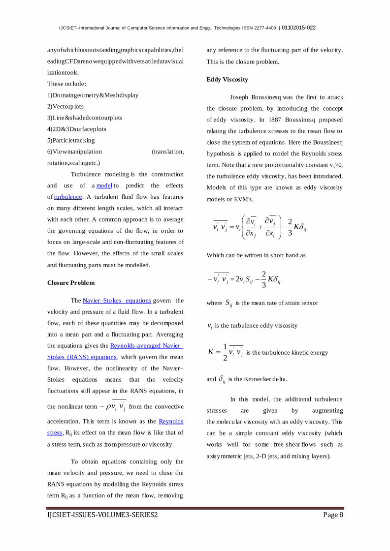
ij

i

j

j

itji K

x

v

x

vvvv

3

2''

Which can be written in short hand as

''

ji vv = ijijt KSv 3

22

where ijS is the mean rate of strain tensor

tv is the turbulence eddy viscosity

''

2

1ji vvK is the turbulence kinetic energy

and ij is the Kronecker delta.

In this model, the additional turbulence

stresses are given by augmenting

the molecu lar v iscosity with an eddy viscosity. This

can be a simple constant eddy viscosity (which

works well for some free shear flows such as

axisymmetric jets, 2-D jets, and mixing layers).

IJCSIET-ISSUE5-VOLUME3-SERIES2 Page 9

IJCSIET--International Journal of Computer Science inf ormation and Engg., Technologies ISSN 2277-4408 || 01102015-022

Prandtl's Mixing-Length Concept

Later, Ludwig Prandtl introduced the

additional concept of the mixing length, along with

the idea of a boundary layer. For wall-bounded

turbulent flows, the eddy viscosity must vary with

distance from the wall, hence the addition of the

concept of a 'mixing length'. In the simplest wall-

bounded flow model, the eddy viscosity is given by

the equation:

2

mt ly

uv

where:

y

u

is the partial derivative of the stream wise

velocity (u) with respect to the wall normal

direction (y);

ml is the mixing length.

This simple model is the basis for the "law

of the wall", which is a surprisingly accurate model

for wall-bounded, attached (not separated) flow

fields with s mall pressure gradients.

More general turbulence models have

evolved over time, with most modern turbulence

models given by field equations similar to

the Navier-Stokes equations.

Smagorinsky Model for the Sub-Grid Scale

Eddy Viscosity

Joseph Smagorinsky (1964) proposed a

useful formula for the eddy viscosity in numerical

models, based on the local derivatives of the

velocity field and the local grid size:

222

2

1

x

v

y

u

y

v

x

uyxvt

Spalart–Allmaras, K–Ε And K–Ω Models

The Boussinesq hypothesis is employed in

the Spalart–Allmaras (S–A), k–ε (k–epsilon),

and k–ω (k–omega) models and offers a relatively

low cost computation for the turbulence

viscosity . The S–A model uses only one

additional equation to model turbulence viscosity

transport, while the k models use two.

k-epsilon turbulence model

K-epsilon (k-ε) turbulence model is the

most common model used in Computational Flu id

Dynamics (CFD) to simulate mean flow

characteristics for turbulent flow conditions. It is a

two equation model which gives a general

description of turbulence by means of two transport

equations (PDEs). The original impetus for the K-

epsilon model was to improve the mixing-length

model, as well as to find an alternative to

algebraically prescrib ing turbulent length scales in

moderate to high complexity flows.

The first transported variable determines

the energy in the turbulence and is called turbulent

kinetic energy (k).

The second transported variable is the

turbulent dissipation (ε) which determines the rate

of dissipation of the turbulent kinetic energy.

Principle

Unlike earlier turbulence models, k-ε

model focuses on the mechanisms that affect the

turbulent kinetic energy. The mixing length

model lacks this kind of generality. The underlying

IJCSIET-ISSUE5-VOLUME3-SERIES2 Page 10

IJCSIET--International Journal of Computer Science inf ormation and Engg., Technologies ISSN 2277-4408 || 01102015-022

assumption of this model is that the turbulent

viscosity is isotropic, in other words, the ratio

between Reynolds stress and mean rate of

deformations is the same in all directions.

Standard k-ε turbulence model

The exact k-ε equations contain many

unknown and unmeasurable terms. For a much

more pract ical approach, the standard k-

ε turbulence model (Launder and Spalding, 1974)

is used which is based on our best understanding of

the relevant processes, thus minimizing unknowns

and presenting a set of equations which can be

applied to a large number of turbulent applicat ions.

For turbulent kinetic energy k

ijijt

jk

t

ji

i EEx

k

xx

ku

t

k2

For dissipation

k

CEEk

Cxxx

u

tijijt

j

t

ji

i

2

21 2

In other words,

Rate of change of k or ε + Transport of k

or ε by convection = Transport of k o r ε

by diffusion + Rate of production of k or

ε - Rate of destruction of k or ε

Where

iu Represents velocity component in

corresponding direction

ijE Represents component of rate of deformat ion

t Represents eddy viscosity

2kCt

The equations also consist of some

adjustable constants 1,, Ck and

2C . The

values of these constants have been arrived at by

numerous iterations of data fitting for a wide range

of turbulent flows. These are as follows:

09.0C 00.1k 30.1

44.11 C 92.12 C

CFD modelling of High Speed

Turbine

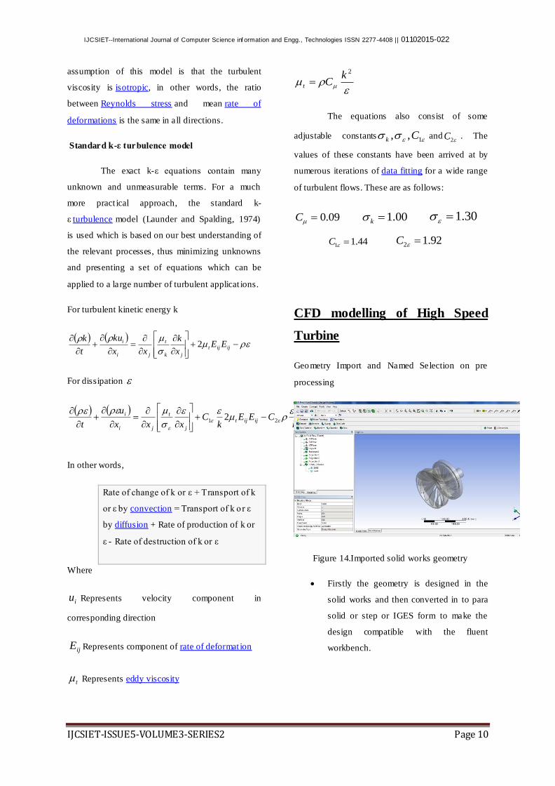
Geometry Import and Named Selection on pre

processing

Figure 14.Imported solid works geometry

Firstly the geometry is designed in the

solid works and then converted in to para

solid or step or IGES form to make the

design compatible with the fluent

workbench.

IJCSIET-ISSUE5-VOLUME3-SERIES2 Page 11

IJCSIET--International Journal of Computer Science inf ormation and Engg., Technologies ISSN 2277-4408 || 01102015-022

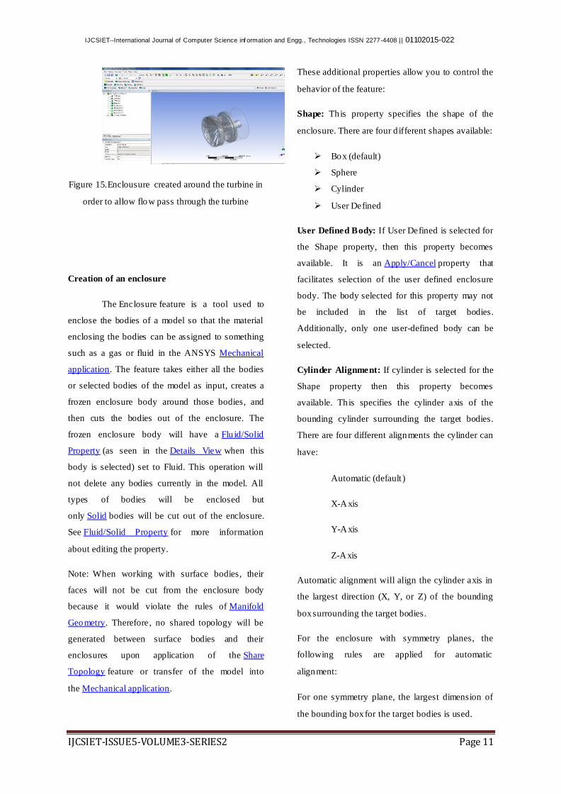
Figure 15.Enclousure created around the turbine in

order to allow flow pass through the turbine

Creation of an enclosure

The Enclosure feature is a tool used to

enclose the bodies of a model so that the material

enclosing the bodies can be assigned to something

such as a gas or fluid in the ANSYS Mechanical

application. The feature takes either all the bodies

or selected bodies of the model as input, creates a

frozen enclosure body around those bodies, and

then cuts the bodies out of the enclosure. The

frozen enclosure body will have a Flu id/Solid

Property (as seen in the Details View when this

body is selected) set to Fluid. This operation will

not delete any bodies currently in the model. All

types of bodies will be enclosed but

only Solid bodies will be cut out of the enclosure.

See Fluid/Solid Property for more information

about editing the property.

Note: When working with surface bodies, their

faces will not be cut from the enclosure body

because it would violate the rules of Manifold

Geometry. Therefore, no shared topology will be

generated between surface bodies and their

enclosures upon application of the Share

Topology feature or transfer of the model into

the Mechanical application.

These additional properties allow you to control the

behavior of the feature:

Shape: Th is property specifies the shape of the

enclosure. There are four d ifferent shapes available:

Box (default)

Sphere

Cylinder

User Defined

User Defined Body: If User Defined is selected for

the Shape property, then this property becomes

available. It is an Apply/Cancel property that

facilitates selection of the user defined enclosure

body. The body selected for this property may not

be included in the list of target bodies.

Additionally, only one user-defined body can be

selected.

Cylinder Alignment: If cylinder is selected for the

Shape property then this property becomes

available. Th is specifies the cylinder axis of the

bounding cylinder surrounding the target bodies.

There are four different alignments the cylinder can

have:

Automatic (default )

X-Axis

Y-Axis

Z-Axis

Automatic alignment will align the cylinder axis in

the largest direction (X, Y, or Z) of the bounding

box surrounding the target bodies.

For the enclosure with symmetry planes, the

following rules are applied for automatic

alignment:

For one symmetry plane, the largest dimension of

the bounding box for the target bodies is used.

IJCSIET-ISSUE5-VOLUME3-SERIES2 Page 12

IJCSIET--International Journal of Computer Science inf ormation and Engg., Technologies ISSN 2277-4408 || 01102015-022

For two symmetry planes, the intersection of the

two symmetry planes is used.

For three symmetry planes, the intersection of the

first two symmetry planes is used.

Number of Planes: This property defines how

many symmetry planes are used in the enclosure.

The default value is 0.

Symmetry Plane1: first symmetry plane selection

Symmetry Plane2: second symmetry plane

selection

Symmetry Plane3: third symmetry p lane selection

Model Type: Th is property specifies either Full

Model or Partial Model as input for the enclosure

with symmetry planes:

Cushion: The cushion property specifies the

distance between the model and the outside of the

enclosure body. The enclosure is initially

calculated to be just big enough to fit the model,

and then the cushion value is applied to make the

enclosure larger. The cushion is set to a default

value and must be greater than zero.

Full Model: ANSYS Design Modeler will use the

chosen symmetry planes to cut the full model,

leaving only the symmetrical portion. For each

symmetry plane, material on the positive side of the

plane (that is, the +Z direction) is kept, while

material on the negative side is cut away.

Partial Model: Since the model has already been

reduced to its symmetrical portion, Design Modeler

will automat ically determine on which side of the

symmetry planes the material lies.

Note: At ANSYS release 12.1, the distance

specified by the cushion property has increased

from 500m to 500Km when the large model

support option is enabled.

Cushion values for Box or Cylinder type enclosures

can be either Uniform or Non-Uniform. Non-

Uniform type accepts different values for X, Y and

Z directions for the Box dimension. Similarly

Cylinder Enclosure takes the cushion values for

radius, positive and negative reference directions.

This property is available for all enclosure shapes

except User Defined. This property may also be set

as a design parameter.

The bounding box calculat ion for the model used in

the Enclosure feature is guaranteed to contain the

model (or selected bodies). While the computed

bounding box is usually very close to the

minimum-bounding box, it is not guaranteed.

Target Bodies: Th is property specifies whether all

of the bodies or only selected bodies of the model

will be enclosed. The default is All Bodies.

Bodies: If Target Bodies is set to Selected Bodies

then this property becomes available. It is

an Apply/Cancel button property that facilitates

selection of the target bodies that you wish to be

enclosed. None of the bodies selected for this

property can also be selected as the user-defined

body.

Merge Parts : Th is property specifies whether or

not the enclosure and its target bodies will be

merged together to form a part. It is only available

during feature creation or while performing Edit

Selections. If Yes, the enclosure body (or bodies)

and all target bodies will be merged into a single

part. Only Solid bodies are considered when

merging parts - line and Surface bodies will not be

merged. If the property is set to no, then no attempt

is made to group the bodies into the same part, nor

is any attempt made to undo any groupings

IJCSIET-ISSUE5-VOLUME3-SERIES2 Page 13

IJCSIET--International Journal of Computer Science inf ormation and Engg., Technologies ISSN 2277-4408 || 01102015-022

previously performed. The Merge Parts property is

set to no by default, and will automatically be set to

no after each Merge Parts operation.

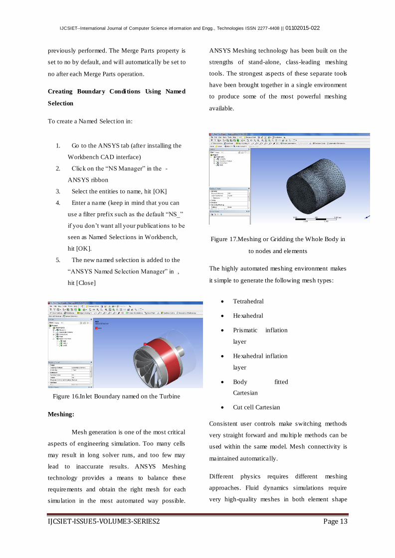
Creating Boundary Conditions Using Named

Selection

To create a Named Select ion in:

1. Go to the ANSYS tab (after installing the

Workbench CAD interface)

2. Click on the “NS Manager” in the -

ANSYS ribbon

3. Select the entities to name, hit [OK]

4. Enter a name (keep in mind that you can

use a filter prefix such as the default “NS_”

if you don‟t want all your publicat ions to be

seen as Named Select ions in Workbench,

hit [OK].

5. The new named selection is added to the

“ANSYS Named Selection Manager” in ,

hit [Close]

Figure 16.In let Boundary named on the Turbine

Meshing:

Mesh generation is one of the most critical

aspects of engineering simulation. Too many cells

may result in long solver runs, and too few may

lead to inaccurate results. ANSYS Meshing

technology provides a means to balance these

requirements and obtain the right mesh for each

simulation in the most automated way possible.

ANSYS Meshing technology has been built on the

strengths of stand-alone, class-leading meshing

tools. The strongest aspects of these separate tools

have been brought together in a single environment

to produce some of the most powerful meshing

available.

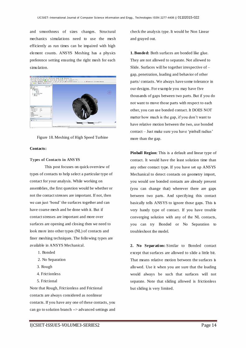
Figure 17.Meshing or Gridding the Whole Body in

to nodes and elements

The highly automated meshing environment makes

it simple to generate the following mesh types:

Tetrahedral

Hexahedral

Prismatic inflation

layer

Hexahedral inflation

layer

Body fitted

Cartesian

Cut cell Cartesian

Consistent user controls make switching methods

very straight forward and multip le methods can be

used within the same model. Mesh connectivity is

maintained automatically.

Different physics requires different meshing

approaches. Fluid dynamics simulations require

very high-quality meshes in both element shape

IJCSIET-ISSUE5-VOLUME3-SERIES2 Page 14

IJCSIET--International Journal of Computer Science inf ormation and Engg., Technologies ISSN 2277-4408 || 01102015-022

and smoothness of sizes changes. Structural

mechanics simulat ions need to use the mesh

efficiently as run times can be impaired with high

element counts. ANSYS Meshing has a physics

preference setting ensuring the right mesh for each

simulation.

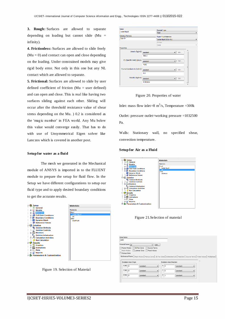
Figure 18. Meshing of High Speed Turbine

Contacts:

Types of Contacts in ANS YS

This post focuses on quick overview of

types of contacts to help select a particular type of

contact for your analysis. While working on

assemblies, the first question would be whether or

not the contact stresses are important. If not, then

we can just „bond‟ the surfaces together and can

have coarse mesh and be done with it. But if

contact stresses are important and more over

surfaces are opening and closing then we need to

look more into other types (NL) of contacts and

finer meshing techniques. The following types are

available in ANSYS Mechanical.

1. Bonded

2. No Separation

3. Rough

4. Frict ionless

5. Frict ional

Note that Rough, Frict ionless and Frictional

contacts are always considered as nonlinear

contacts. If you have any one of these contacts, you

can go to solution branch --> advanced settings and

check the analysis type. It would be Non Linear

and grayed out.

1. Bonded: Both surfaces are bonded like glue.

They are not allowed to separate. Not allowed to

Slide. Surfaces will be together irrespective of –

gap, penetration, loading and behavior of other

parts/ contacts. We always have some tolerance in

our designs. For example you may have five

thousands of gaps between two parts. But if you do

not want to move those parts with respect to each

other, you can use bonded contact. It DOES NOT

matter how much is the gap, if you don‟t want to

have relative motion between the two, use bonded

contact – Just make sure you have „pinball radius‟

more than the gap.

Pinball Region: This is a default and linear type of

contact. It would have the least solution time than

any other contact type. If you have set up ANSYS

Mechanical to detect contacts on geometry import,

you would see bonded contacts are already present

(you can change that) wherever there are gaps

between two parts. And specifying this contact

basically tells ANSYS to ignore those gaps. This is

very handy type of contact. If you have trouble

converging solution with any of the NL contacts,

you can try Bonded or No Separation to

troubleshoot the model.

2. No Separation: Similar to Bonded contact

except that surfaces are allowed to slide a little bit.

That means relative motion between the surfaces is

allowed. Use it when you are sure that the loading

would always be such that surfaces will not

separate. Note that sliding allowed is frictionless

but sliding is very limited.

IJCSIET-ISSUE5-VOLUME3-SERIES2 Page 15

IJCSIET--International Journal of Computer Science inf ormation and Engg., Technologies ISSN 2277-4408 || 01102015-022

3. Rough: Surfaces are allowed to separate

depending on loading but cannot slide (Mu =

infinity).

4. Frictionless: Surfaces are allowed to slide freely

(Mu = 0) and contact can open and close depending

on the loading. Under constrained models may give

rig id body error. Not only in this one but any NL

contact which are allowed to separate.

5. Frictional: Surfaces are allowed to slide by user

defined coefficient of friction (Mu = user defined)

and can open and close. This is real like having two

surfaces sliding against each other. Slid ing will

occur after the threshold resistance value of shear

stress depending on the Mu. ) 0.2 is considered as

the „magic number‟ in FEA world. Any Mu below

this value would converge easily. That has to do

with use of Unsymmetrical Eigen solver like

Lanczos which is covered in another post.

Setup for water as a fluid

The mesh we generated in the Mechanical

module of ANSYS is imported in to the FLUENT

module to prepare the setup for fluid flow. In the

Setup we have different configurations to setup our

flu id type and to apply desired boundary conditions

to get the accurate results.

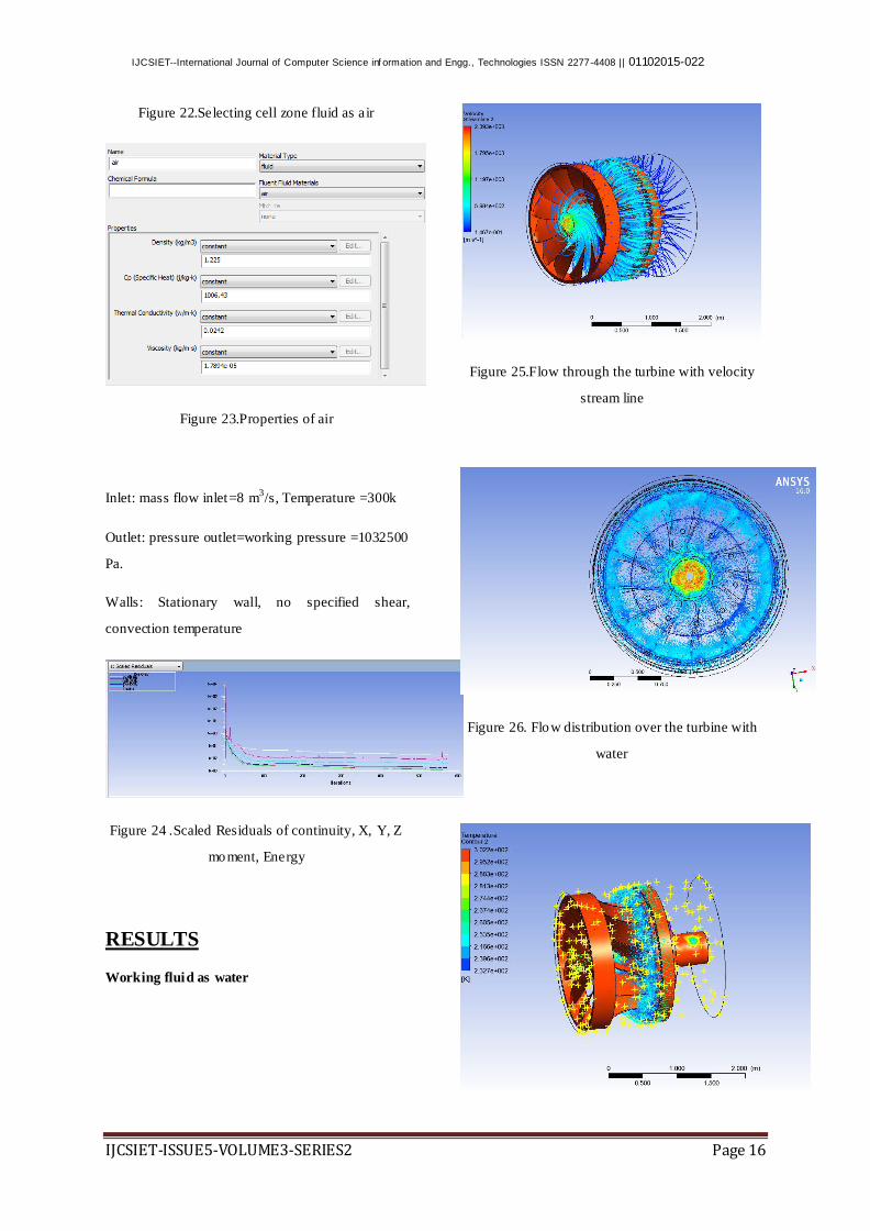
Figure 19. Selection of Material

Figure 20. Properties of water

Inlet: mass flow inlet=8 m3/s, Temperature =300k

Outlet: pressure outlet=working pressure =1032500

Pa.

Walls: Stationary wall, no specified shear,

convection temperature.

Setup for Air as a Fluid

Figure 21.Selection of material

IJCSIET-ISSUE5-VOLUME3-SERIES2 Page 16

IJCSIET--International Journal of Computer Science inf ormation and Engg., Technologies ISSN 2277-4408 || 01102015-022

Figure 22.Selecting cell zone fluid as air

Figure 23.Properties of air

Inlet: mass flow inlet=8 m3/s, Temperature =300k

Outlet: pressure outlet=working pressure =1032500

Pa.

Walls: Stationary wall, no specified shear,

convection temperature

Figure 24 .Scaled Residuals of continuity, X, Y, Z

moment, Energy

RESULTS

Working fluid as water

Figure 25.Flow through the turbine with velocity

stream line

Figure 26. Flow distribution over the turbine with

water

IJCSIET-ISSUE5-VOLUME3-SERIES2 Page 17

IJCSIET--International Journal of Computer Science inf ormation and Engg., Technologies ISSN 2277-4408 || 01102015-022

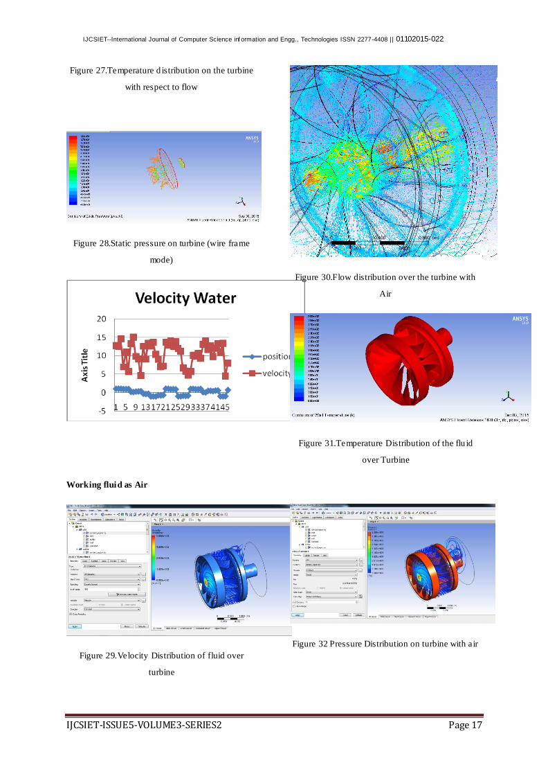
Figure 27.Temperature d istribution on the turbine

with respect to flow

Figure 28.Static pressure on turbine (wire frame

mode)

Working fluid as Air

Figure 29.Velocity Distribution of fluid over

turbine

Figure 30.Flow distribution over the turbine with

Air

Figure 31.Temperature Distribution of the flu id

over Turbine

Figure 32 Pressure Distribution on turbine with air

IJCSIET-ISSUE5-VOLUME3-SERIES2 Page 18

IJCSIET--International Journal of Computer Science inf ormation and Engg., Technologies ISSN 2277-4408 || 01102015-022

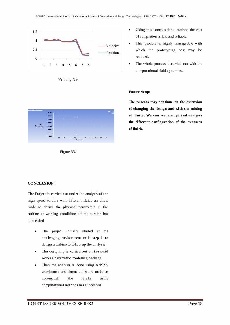
Velocity Air

Figure 33.

CONCLUS ION

The Project is carried out under the analysis of the

high speed turbine with different fluids an effort

made to derive the physical parameters in the

turbine at working conditions of the turbine has

succeeded

The project initially started at the

challenging environment main step is to

design a turbine to follow up the analysis.

The designing is carried out on the solid

works a parametric modelling package.

Then the analysis is done using ANSYS

workbench and fluent an effort made to

accomplish the results using

computational methods has succeeded.

Using this computational method the cost

of completion is low and reliable.

This process is highly manageable with

which the prototyping cost may be

reduced.

The whole process is carried out with the

computational fluid dynamics.

Future Scope

The process may continue on the extension

of changing the design and with the mixing

of fluids. We can see, change and analyses

the different configuration of the mixtures

of fluids.