Embed Size (px)
Citation preview

Project No. 3-75 Copy No. 1
ANALYSIS OF FREEWAY WEAVING SECTIONS
FINAL REPORT
Prepared for National Cooperative Highway Research Program
Transportation Research Board National Research Council
Transportation Research Institute
Polytechnic University Six Metrotech Center Brooklyn, NY 11201
and
Kittelson & Associates, Inc.
610 SW Alder Street, Suite 700 Portland, Oregon 97205
January 2008

ACKNOWLEDGMENT OF SPONSORSHIP
This work was sponsored by the American Association of State Highway and Transportation Officials, in cooperation with the Federal Highway Administration, and was conducted in the National Cooperative Highway Research Program, which is administered by the Transportation Research Board of the National Research Council.
DISCLAIMER This is an uncorrected draft as submitted by the research agency. The opinions and conclusions expressed or implied in the report are those of the research agency. They are not necessarily those of the Transportation Research Board, the National Research Council, the Federal Highway Administration, the American Association of State Highway and Transportation Officials, or the individual states participating in the National Cooperative Highway Research Program.

i
TABLE OF CONTENTS
CHAPTER 1 - OVERVIEW, HISTORY, AND CONCEPTS ....................................................... 1 PROJECT OBJECTIVES AND PRODUCTS...........................................................................................................1 HISTORY AND BACKGROUND ...........................................................................................................................2 THE HCM2000 WEAVING ANALYSIS MODEL..................................................................................................7 AN OVERVIEW OF THE RECOMMENDED MODEL .......................................................................................10 CONCEPTS, TERMINOLOGY, AND VARIABLES............................................................................................11 THE DATA BASE ..................................................................................................................................................19 CLOSING COMMENTS ........................................................................................................................................21 REFERENCES FOR CHAPTER 1 .........................................................................................................................22
CHAPTER 2 - PREDICTION OF LANE-CHANGE PARAMETERS....................................... 25
PREDICTING THE RATE OF WEAVING LANE CHANGES IN A WEAVING SECTION .............................25 PREDICTING THE RATE OF NON-WEAVING LANE CHANGES IN A WEAVING SECTION ...................31 CLOSING COMMENTS ........................................................................................................................................39
CHAPTER 3 - PREDICTION OF SPEED PARAMETERS ....................................................... 41
THE HCM2000 MODEL ........................................................................................................................................41 PREDICTING THE AVERAGE SPEED OF WEAVING VEHICLES .................................................................43 PREDICTING THE AVERAGE SPEED OF NON-WEAVING VEHICLES........................................................46 THE ISSUE OF FREE-FLOW SPEED...................................................................................................................51 SENSITIVITY OF SPEED......................................................................................................................................53 CLOSING COMMENTS ........................................................................................................................................59
CHAPTER 4 - CAPACITY OF FREEWAY WEAVING SECTIONS ....................................... 61
THE HCM2000 APPROACH .................................................................................................................................61 CAPACITY OF WEAVING SECTIONS IN THE DATA BASE ..........................................................................62 ESTIMATING WEAVING SECTION CAPACITY ..............................................................................................64 OTHER LIMITATIONS ON CAPACITY..............................................................................................................67 MAXIMUM LENGTH OF WEAVING SECTIONS..............................................................................................70 SENSITIVITY OF CAPACITY..............................................................................................................................71 CLOSING COMMENTS ........................................................................................................................................73
CHAPTER 5 - CONCLUSIONS AND RECOMMENDATIONS............................................... 77
A RECOMMENDED METHODOLOGY ..............................................................................................................77 TWO-SIDED WEAVING SECTIONS ...................................................................................................................83 OTHER RECOMMENDATIONS ..........................................................................................................................84
APPENDIX I - AERIALS & SCHEMATIC OF SITES .............................................................. 87 APPENDIX II – DRAFT CHAPTER FOR THE HCM 2010 .................................................... 103 APPENDIX III – RESPONSES TO REVIEWER COMMENTS.............................................. 159

ii

1
National Cooperative Highway Research Program Project 3-75 ANALYSIS OF FREEWAY WEAVING SECTIONS
Final Report
CHAPTER 1 - OVERVIEW, HISTORY, AND CONCEPTS This document represents the Final Report of the Project Team for National Cooperative Highway Research Program Project 3-75, Analysis of Freeway Weaving Sections. The Project Team includes individuals from the prime contractor, the Transportation Research Institute of Polytechnic University, and a major subcontractor, Kittelson and Associates, Inc. When the project was initiated, a second subcontractor was included, Catalina Engineering, Inc. Catalina subsequently merged into Kittelson and Associates. The Project Team consists of: Polytechnic University Roger P. Roess, Professor of Transportation Engineering (PI) Jose M. Ulerio, Industry Associate Professor of Transportation Engineering Elena S. Prassas, Associate Professor of Transportation Engineering Kittelson and Associates Inc. Jim Schoen, Vice-President (Co-PI) Mark Vandehey, Principal Engineer William Reilly, Principal Engineer Wayne Kittelson, President and Principal Engineer In the early stages of the project, Dr. Alexander Skabardonis of the University of California at Berkeley participated as a consultant. PROJECT OBJECTIVES AND PRODUCTS NCHRP Project 3-75, Analysis of Freeway Weaving Sections has had a clear and focused primary objective: calibrate new and/or updated models for prediction of performance in freeway weaving sections, and draft a replacement chapter for the Highway Capacity Manual. The Project Team, working with the Project Panel and the Highway Capacity and Quality of Service Committee of the Transportation Research Board (HCQSC), established the following desirable characteristics that the new models should embody:
1. The new model(s) should be conceptually logical. 2. The new model(s) should be based on a significant modern data base covering a
broad range of weaving designs, configurations, and demand flow rates. 3. The new model(s) should attempt to eliminate the need for separate algorithms based
upon weaving configuration type and constrained vs. unconstrained operation. 4. The new model(s) should attempt to incorporate parametric measures that directly
describe the impact of configuration, and (if possible) constrained vs. unconstrained operation.
5. The new model(s) should provide demonstrably improved predictions of performance parameters when compared to the current models of the HCM2000.

2
Once such models were developed, the following products were to be prepared:
1. A draft replacement Chapter 24, Freeway Weaving, for the Highway Capacity Manual.
2. Draft material to replace freeway weaving portions of HCM Chapter 13, Freeway Concepts.
3. Recommendations for changes in other related chapters of the HCM, including, but not limited to Chapter 22, Freeway Facilities and Chapter 25, Ramps and Ramp Junctions.
4. A spreadsheet-based computational engine that replicates the methodology developed for freeway weaving sections.
5. A Final Report documenting the research efforts leading to the new model(s) and methodology.
This report provides a detailed explanation of how and why models were developed, and
how they fit together to provide a cohesive methodology for analysis of freeway weaving sections. HISTORY AND BACKGROUND With the possible exception of signalized intersections, it is doubtful that any methodology of the Highway Capacity Manual has been so frequently studied, and so frequently a subject of technical controversy. It is, therefore, beneficial to place this current effort into the historical context of research in the general area of freeway weaving section capacity and performance.
Table 1-1 provides a capsule summary of various approaches that have been used to model freeway weaving areas, beginning with the work leading to the 1965 HCM model – the first to specifically address weaving behavior. The 1965 HCM actually contained two approaches to freeway weaving areas, as part of a model that attempted to address weaving on all types of facilities. The primary model, developed by Leisch and Normann [1], was based upon a set of curves that plotted total weaving volume vs. weaving length. Each curve represented a “k-factor” that varied from 1.0 to 3.0, and was used as a multiplier to develop an “equivalent non-weaving volume” according to the following equation:
2)1( wEQ vkvv −+= where: vEQ = total equivalent non-weaving flow rate, veh/h. v = total flow rate, veh/h (unadjusted) k = weaving intensity factor vw2 = smaller weaving flow rate, veh/h

3
Table 1-1 Summary of Alternative Modeling Approaches to Freeway Weaving Areas
Model Basic Type
Address Capacity?
Address LOS? MOE Comments
Leisch, Normann 1965
Macroscopic, Equivalent Non-
Weaving Vehicles
Not directly. Yes Approx. Speed
Based on very sparse data. Quality of Flow used to map into LOS. Approach not successfully calibrated in later studies.
Hess 1963
Macroscopic, Lane Distribution
Yes Freeway Capacity Controls
Yes Merge, Diverge,
and Freeway Volume
Regression-based model focuses on lane 1 of the freeway and the ramp, general LOS criteria based upon flow rates loosely tied to verbal description of operating characteristics.
Moscowitz & Newman
1963
Microscopic, Lane Distribution
and Lane-Changing by Cell
Yes Freeway Capacity Controls
Yes
Merge, Diverge, Weaving, and
Freeway Volume
Focus on high-volume cell among freeway lane 1 and auxiliary lane, general LOS criteria based upon flow rates loosely tied to verbal description of operating characteristics.
Roess & McShane 1973-1980
Macroscopic, Regression
Based, Speed Prediction
Not directly. Yes
Average Speed of Weaving and Non-Weaving
Vehicles
Appeared in several forms, with final form appearing in Circular 212, iterative process, introduced configuration and type of operation into the analysis process.
Leisch 1983
Macroscopic, Equivalent Non-
Weaving Vehicles
Not directly. Yes Average Speed
A re-calibration of the 1965 Leisch/Normann work. Nomographs used.

4
Table 1-1 (Continued) Summary of Alternative Modeling Approaches to Freeway Weaving Areas
Model Basic Type
Address Capacity?
Address LOS? MOE Comments
Reilly et al 1984
Macroscopic, Theoretical and
Regression-Based,
Speed Prediction
Not directly. Yes
Average Speed of Weaving and Non-Weaving
Vehicles
Introduced a different “density” concept tied to weaving intensity, introduced basic model form still used in HCM 2000.
1985 HCM Roess et al
Macroscopic Not directly. Yes
Average Speed of Weaving and Non-Weaving
Vehicles
Developed as a merger of the earlier Roess/McShane and Reilly models. The Reilly model form was stratified to consider configuration and type of operation.
Fazio 1985
Macroscopic,
Theoretical and Regression-
Based
Not directly. Yes
Average Speed of Weaving and Non-Weaving
Vehicles
Added lane-changing parameter to Reilly-type model, eliminating the need for different configuration types to be considered.
Cassidy, Skabardonis, May, Ostrom
1988-1995
Microscopic, Lane-Distribution
and Lane-Changing by Cell
Yes, Based on Max Cell Flow Rates and Max Lane-Changing
per Cell
Yes Density
A modern look at the Moscowitz/Newman model form, with far greater precision. Lane distribution modeled for each component flow of the weaving section.
HCM 2000 Roess et al Macroscopic Yes Yes Density Addition of density model and capacity
predictions to 1985 HCM methodology.
Lertworawanich & Elefteriadou
2001-2002
Microscopic, Gap Acceptance
and Linear Programming
Yes No N/A
Capacity model based upon gap acceptance and linear programming optimization treats weaving capacity as function of basic freeway capacity.

5
The 1965 HCM model did not refer to the term “equivalent non-weaving volume” or flow rate. The algorithm was, however, used to determine the number of lanes needed in the weaving section, essentially dividing vEQ by an appropriate capacity or service volume per lane.
NCHRP 3-15, Weaving Area Operations Study, conducted at Polytechnic University [2] in the early 1970’s made extensive attempts to calibrate the weaving curves of the 1965 HCM. Calibrated k-factors, however, could not be systematically related to the length of the weaving section and weaving volume or flow rate, even when different constructs of the “equivalent non-weaving volume” concept were attempted. Another unique aspect of the 1965 HCM model was the clear definition of “out of the realm of weaving.” The weaving curve for a k-factor of 1.0 essentially identified the limit of weaving length that resulted in weaving movements. Beyond these lengths, which depended upon weaving volume or flow rate, the section was believed to operate as a basic freeway section, with merging at one end and diverging at the other. The curve depicted lengths of up to 8,000 ft, based largely on data from a single long weaving site. Subsequent weaving studies have focused on lengths no longer than 3,000 – 3,500 ft, due to the cost of data collection and the likelihood that longer sections do not operate as weaving sections. The issue of maximum length of weaving sections is addressed as part of the current research. The 1965 HCM contained another model that could be applied to ramp-weave configurations. The model, developed by Moskowitz and Newman [3], was actually presented as a merging and diverging model for ramp junctions operating at levels of service D and E. It defined lane-changing distributions between lane 1 (right freeway lane) and the auxiliary lane, and identified the 500-ft segment that had the most intense lane-changing activity. This model provides the theoretic basis for subsequent algorithms based upon microscopic lane-changing of other characteristics. The primary weakness of the model was that the lane-changing distribution was based solely on the length of the section, and did not vary with other factors, such as volume or flow rate, or the split between weaving movements. The first significant post-1965 HCM study of weaving sections was NCHRP Project 3-15. It was also the first in a string of NCHRP and FHWA-sponsored efforts directed specifically towards the development of the 1985 HCM (which was originally supposed to be the 1983 HCM). The results of NCHRP 3-15, Weaving Area Operations Study, were published in an NCHRP Report [4]. The model introduced the issue of configuration, and involved complex iterations. As part of an FHWA-sponsored study of Freeway Capacity Analysis in the late 1970’s, the model was re-formatted by Roess and McShane and published in TRB Circular 212 [5], Interim Materials on Highway Capacity. This model continued to be complex and iterative, but broke the original model into discrete steps that were more easily explained and implemented. It also introduced the concept of constrained vs. unconstrained operation, even to the point of defining the degree of constraint that might exist.
While some of the concepts of this model were interesting, and survive in current models, the algorithms were difficult to implement, and their subdivision into various components made calibration an issue, given the limited size of the data bases available at the time.

6
While the NCHRP and FHWA studies progressed, Leisch [6] independently developed a model similar to the 1965 HCM in form and concept. FHWA later funded the documentation of the method. In the meantime, the model was also published as part of TRB Circular 212. Thus, from 1980 through the publication of the 1985 HCM, several different weaving area analysis methodologies were in active use: the two models from the 1965 HCM, the Roess/McShane method of Circular 212, and the Leisch method of Circular 212. The Leisch model continued to depict weaving lengths for which no data existed, and produced results that differed substantially from the Roess/McShane model, even though both were calibrated with the same data. In 1981, another weaving research effort was launched to answer the question of whether the Roess/McShane model or the Leisch model should be chosen for the forthcoming 1985 HCM. Conducted by JHK and Associates, the study included additional data collection, and recommended a third model for inclusion in the HCM. This model, developed by Reilly et al [7], resulted in the algorithm form that is currently used in the HCM2000. The model did not, however, address configuration or type of operation. The 1985 HCM model was based upon the Reilly algorithm, modified by Roess (at the behest of the HCQSC) to incorporate the impact of configuration and type of operation. The model has been updated twice since 1985, based upon a single data base from the Reilly study consisting of 10 sites with 1 hour of data each. Both revisions were made to constants of calibration in the primary algorithm, and were published in the 1994 update to the manual and HCM2000. Other changes in the HCM2000 included the elimination of multiple weaving area analysis, the development of a complex capacity estimation procedure, and conversion to a density-based level of service definition. Since 1985, a number of additional weaving area studies have taken place. All were handicapped by small data bases, but a number of interesting concepts resulted. Fazio [8] developed a model around the Reilly algorithm, but added a lane-changing parameter that eliminated the need to pre-categorize weaving areas by configuration. This is essentially the approach recommended herein, with more attention paid to the development of the lane-changing parameter(s). Fazio, due to a small data base, was forced to assume entry lane-distribution behavior of weaving vehicles to estimate lane-changing.
CALDOT and the University of California at Berkeley conducted a number of weaving studies through the 1980’s and early 1990’s that focused on recalibration of a model similar to the Moskowitz/Newman approach in the 1965 HCM [9, 10, 11, 12].
Over the years, several different calibrations were researched by CALDOT/Berkeley. The methodology(ies) have both strengths and weaknesses. All of the configurations studied in the California work would be classified (in the original terms of the 1965 HCM) as one-sided weaving sections in which weaving activity is focused on the right-most lanes of the section. Two-sided weaving sections were not included in the studies. A major issue is the calibration of lane distribution models.

7
Given that separate distributions are needed for each of several lanes, for three or four component flows (including ramp-to-ramp), and for various lengths and configurations, the number of such models needed to cover the full range of weaving sections is extremely large. An alternative approach that might be simpler would be to focus entirely on the prediction of critical cell characteristics using general models in which length of section, flow parameters, and configuration parameters are included. While this approach has led to some success in replicating field observations of weaving operations, the difficulty and cost of collecting and reducing a data base sufficient to calibrate the many independent algorithms needed caused the Project Team to follow a macroscopic approach requiring far less data for calibration. In a doctoral dissertation by P. Lertworawanich and two papers by Lertworawanich and L. Elefteriadou [13, 14, 15], a methodology for estimating the capacity of ramp-weave and major weave sections is developed based upon linear optimization and gap acceptance modeling. The methodology, while theoretically reasonable, has its greatest difficulty in the application of gap acceptance parameters to implement the final two constraints. First, gap acceptance models are taken from publications of Drew et al in 1967 and Raff and Hart in 1950. Neither of these publications is relevant to modern freeway flow characteristics. To implement these models, the speeds of weaving and non-weaving vehicles were needed as inputs; the researchers estimated these from the models of the 2000 HCM. THE HCM2000 WEAVING ANALYSIS MODEL
The core algorithm in the capacity and level of service analysis of weaving sections has been the prediction of average operating speeds (separately for weaving and non-weaving vehicle streams) within the section since 1985. In the 1985HCM, and its subsequent update in 1994, speed was directly related to level of service. In the 1997 update, and in the HCM2000, speed was predicted and subsequently converted to density to determine level of service. The conversion to density was made to provide consistency with level of service methodologies for basic freeway sections and ramp junctions. In terms of the methodology, however, the principal predictive algorithm determined the average speeds of weaving and non-weaving vehicles in the weaving section.
Previous to that, the methodology of the 1965HCM relied upon a set of loosely-defined “Quality of Flow” definitions that were generally related to speed ranges. The speed-prediction algorithm was originally developed by Reilly et al as part of an FHWA-sponsored research effort in 1983-1984, “Weaving Analysis Procedures for the New Highway Capacity Manual.” The “new” manual referred to was the 1985HCM, then under development.

8
The form of the algorithm recommended was:
⎥⎥⎥⎥⎥
⎦
⎤
⎢⎢⎢⎢⎢
⎣
⎡
⎟⎟⎠
⎞⎜⎜⎝
⎛ ++
−+=
d
cbi
LNvVRa
SSSS)/(*)1(*1
minmaxmin
where: Si = speed being predicted, mph (w = speed of weaving vehicles; nw = speed of non-weaving vehicles) Smin = minimum possible speed prediction, mph Smax = maximum possible speed prediction, mph VR = volume ratio; ratio of weaving flow rate to total flow Rate v = total flow rate, pc/h N = number of lanes in the weaving section L = length of the weaving section, ft a, b, c, d = constants of calibration The Reilly study recommended that two equations be used: one for prediction of average weaving vehicle speed in a weaving section, and another for prediction of average non-weaving vehicle speed in a weaving section. The data base for the Reilly study consisted of 10 hours of data from 10 weaving sites. Weaving speeds varied from 40.9 mph to 63.0 mph, and non-weaving speeds varied from 43.9 mph to 63.5 mph. These ranges are important, as they suggest that all of the data derived from stable flow periods. Lengths varied from 800 ft to 3,540 ft, and all sections consisted of 4 lanes. Each of the three defined configuration types was included. The Reilly study also made use of an earlier data base consisting of 45 hours of data from 45 sites, most of it from a 1963 study conducted by the then Bureau of Public Roads, with additional data from a 1973 NCHRP study conducted at Polytechnic University. The calibrated algorithms from the Reilly study resulted in the following parameters: For Weaving Speed: Smin = 15 mph Smax = 65 mph a = 1/2.2 = 0.455 b, c, d = 2.5 R2 = 0.88

9
For Non-Weaving Speed: Smin = 15 mph Smax = 65 mph a = 1/3.9 = 0.256 b, c, d = 2.4 R2 = 0.74 The calibrated equations had a number of very desirable characteristics. They could only predict a speed between 15 and 65 mph, thus bounding the results to a reasonable range. The form of the equation guaranteed appropriate sensitivities (as long as the exponents b, c, and d were positive). On the negative side, the calibration for a speed range of 15 mph to 65 mph relied only on data between approximately 40 mph and 63 mph, providing no check on its accuracy in the prediction of lower speeds. When the same equations were calibrated using the older data base of 45 sites, the results were poor, with R2 values ranging between 0.20 and 0.30. The difficulty with the almost 20-year gap in the age of the data, however, tempers this result. The driving habits on U.S. freeways certainly changed remarkably over the period 1963 to 1983. The weaving chapter of the 1985HCM was the last to be written. The results of the Reilly study left the HCQSC with three options on the table: (1) a procedure developed by Polytechnic University in 1973 and modified in 1978, (2) a procedure developed by Jack Leisch in 1980, and (3) the Reilly procedure described above. The committee opted to go with the form of the algorithm developed by Reilly et al, with modifications to reflect the impact of configuration types (included in the Polytechnic and Leisch methodologies), and the issue of constrained and unconstrained operation (included in the Polytechnic methodology). Final “calibrations” were conducted at Polytechnic University, which had the NCHRP contract (3-28B) to develop the 1985HCM. The recalibrations to incorporate the impacts of constrained vs. unconstrained operation and configuration relied on the 10 data sets from the Reilly study, and resulted in six equations for the prediction of weaving speed, and six for non-weaving speed. The six equations were for prediction of speeds for three configuration types, and for constrained vs. unconstrained operation. This explains why the word “calibrations” is in quotations. Six different equations had to be developed from a data base of 10 points! Since the data base was statistically inadequate to support such development, a trial-and-error approach was taken until prediction results demonstrably better than the Reilly model were achieved for the ten newest data sets, and the sensitivities to key variables were logical. This is important, because the last time a formal regression analysis on weaving data was performed was as part of the Reilly study. All subsequent development was in the form of “tinkering” with the base algorithm to provide better predictions for the 10 most recent data sets available at the time. More “tinkering” was done, resulting in changes in the calibration coefficients in both 1993 and 1997. With no new field data available, both were based upon the 10 data sets from 1983. In 1997, the maximum speed of 65 mph was replaced with the free-flow speed plus 5 mph (an adjustment for the tendency of the model to under predict high speeds).

10
AN OVERVIEW OF THE RECOMMENDED MODEL Figure 1-1 shows a flow chart of the methodology that has been developed as a result of this research. In some ways, the methodology is not radically different from the HCM2000 approach. There are two major differences that should be noted:
1. There is no segregation of algorithms based upon weaving configuration, or constrained vs. unconstrained operation. There is a single algorithm for predicting the average speed of weaving vehicles, and a single algorithm for predicting the average speed of non-weaving vehicles.
2. Level of Service F is identified when the ratio of arrival (or demand) flow rate
exceeds capacity of the weaving section. This is similar to the approach in the Basic Freeway Section and Ramp Junction models of the HCM2000.
If v/c ≤ 1.00, continue to Step 5.
STEP 1:Identify demand volumes by movement and vehicle type, and specify the section geometry completely.
STEP 2:Convert all input volumes to 15-minute flow rates in pcph.
STEP 3:Estimate the number of weaving and non-weaving lane-change made in the section. (New predictive algorithm).
STEP 7:Compare input data and output results to maxima and minima stated for the methodology. (Revised and/or new criteria).
STEP 6:Convert speeds to an average density for the weaving section, and determine level of service.
STEP 5:Estimate the average speed of weaving and non-weaving vehicles in the weaving section. (Revised Algorithms)
STEP 4:Estimate the capacity of the section and the v/c ratio for the existing or projected flow conditions. (New predictive algorithm).
If v/c > 1.00, LOS F
Figure 1-1
Flow Chart of the Recommended Methodology

11
The former, however, requires that parameters predicting the total lane-changing activity expected in the weaving section be predicted. This introduces a new set of concepts, parameters, and algorithms to the methodology, as noted in Step 3 of Figure 1-1.
The latter requires that the capacity of the weaving section be predicted in a more
straightforward fashion. An updated methodology for doing so has been developed, and is noted as Step 4 of Figure 1-1. Other aspects of the model will be familiar. All algorithms are based upon flow rates in pc/h/ln, with the standard analysis period remaining 15 minutes. For stable flow situations, speeds of weaving and non-weaving vehicles will be estimated and converted to an average speed for all vehicles, and subsequently, an average density that determines level of service.
CONCEPTS, TERMINOLOGY, AND VARIABLES For obvious reasons, the proposed algorithms use, for the most part, the same terminology and variables as in the HCM2000 – which are, themselves, mostly the same as those used since 1965. Because the recommended methodology relies on a number of new variables and concepts, these need to be precisely defined and consistently used.
Things That Don’t Change There are a number of basic variables that do not change in the recommended methodology. For completeness, they are summarized and defined here: v = total flow rate in the weaving section, pc/h (v = vNW + vW) vW = flow rate of weaving vehicles in the weaving section, pc/h vNW = flow rate of non-weaving vehicles in the weaving section, pc/h SW = average speed of weaving vehicles in the weaving section, mi/h SNW = average speed of non-weaving vehicles in the weaving section, mi/h S = average (space mean) speed of all vehicles in the weaving section, mi/h D = density of all vehicles in the weaving section, pc/mi/ln VR = volume ratio, vW/v Note that length is not included on this list, as its exact meaning will change (see next section). The weaving ratio, R, will no longer be used in the methodology, as it did not have a significant impact on any of the calibrations, and is no longer needed. Several new concepts with respect to lane-changing activity must also be introduced.
The Length of a Weaving Section The HCM2000 includes a methodology for measurement of the length of a weaving section that is more historic than logical. It measures the length of a weaving section from a point on the entry gore where the right-most edge of the freeway traveled pavement is 2 feet from the left-most edge of the ramp traveled pavement to a point on the exit gore where these edges are 12 feet apart.

12
Most likely, this definition dates to the earliest days of highway capacity analysis, when weaving sections were most often found between the loop ramps of a cloverleaf interchange. Given design practices of the day, the exit loop generally diverted at a harsher angle than the entry loop merged. In modern terms, weaving sections are no longer dominated by this case, and the definition seems poorly suited to modern analysis. The Project Team worked with four different definitions of length, as illustrated in Figure 1-2.
LS
LB
LL
Figure 1-2 Measurement of Weaving Length Illustrated
The lengths illustrated in Figure 1-2 are defined as follows:
LS = Short Length, ft; the distance between the end points of any barrier markings that prohibit or discourage lane-changing.
LB = Base Length; ft; the distance between points in the respective gore areas
where the left edge of the ramp travel lanes and the right edge of the freeway travel lanes meet.
LL = Long Length, ft; the distance between physical barriers marking the ends
of the merge and diverge gore areas. A fourth length, LA = average length (ft), was defined as the average of LB and LS. At this time, the use of LS as the defining length has significantly improved the statistical fit to data in algorithms that include a length measure. This is not to say that LS defines the length actually used for lane-changing by weaving and/or non-weaving vehicles. Video evidence suggests that barrier lines are not well observed in the field, although such markings do tend to induce less last-minute lane-changing near the gore areas. From videos of lane-changing maneuvers in the data base, it appears that LB would be the most logical measure of length, but the statistical analysis has not sustained this impression.

13
Depending upon the specific design and marking of a weaving section, some of these values might be equal, but in many cases they are not. Particularly where analysis of future designs are involved, it might be difficult to know what the eventual value of LS will be. From the data base used for this study, on average LS was 88% of LB. If sites where the two measures were the same are eliminated, LS was 77% of LB. These might form the basis of a default value for use where the details of striping are not yet known.
Capacity Terminology The standard capacity terminology will have to be greatly expanded in the new weaving chapter. In general, the manual uses the simple term c, which signifies the total capacity of a freeway section in veh/h under prevailing conditions. In the recommended weaving methodology, we have to deal with both total capacities and capacities per lane in both a weaving section, and on a comparable basic freeway sections (with the same free-flow speed). Further, these values have to be stated in terms of equivalent pc/h for ideal conditions, as well as in terms of veh/h under prevailing conditions. In all cases, capacities are stated as flow rates for a peak 15-minute period, which is consistent with current usage in the HCM. If subscripts are used systematically, we can define the following: I = subscript indicating a capacity under ideal conditions in pc units. L = subscript indicating a capacity per lane. F = subscript indicating a capacity for a basic freeway section of the same free-flow speed as the weaving section. W = subscript indicating a capacity for the weaving section. Using this system: cIFL = capacity per lane of a basic freeway section under ideal conditions (pc/h/ln) cIWL = capacity per lane, weaving section (pc/h/ln) cIW = total capacity of the weaving section under ideal conditions (pc/h) (cIW = cIWL x N) cW = total capacity of the weaving section under prevailing conditions (veh/h) (cW = cIWL x N x fHV x fp) and so forth. While a simpler system might be desirable, these symbols must remain consistent with usage throughout the HCM2000, while at the same time being readily distinguishable from each other.
Critical Lane-Changing Concepts Because lane-changing activity will be such a significant factor in the methodology, there are several new variables that have to be introduced, and two new concepts which have to be clearly defined. Five new variables, each describing lane-changing activity in the weaving section, are introduced:

14
LCW = total number of lane changes made by weaving vehicles in a weaving section, expressed as an hourly rate, lc/h.
LCNW = total number of lane changes made by non-weaving vehicles in a weaving
section, expressed as an hourly rate, lc/h. LCALL = total number of lane changes made by all vehicles in a weaving section,
expressed as an hourly rate, lc/h. (LCALL = LCW + LCNW) LCMIN = minimum number of lane changes that must be made by weaving vehicles
in order to successfully execute their desired weaving maneuver, expressed as an hourly rate, lc/h.
NWL = number of lanes from which (NOT to which) a weaving movement may be
made with a single lane change, referred to as “weaving lanes.” The last two involve significant new concepts. LCMIN is found by assuming that all weaving vehicles enter the weaving section in the lane closest to their destination, and leave the weaving section in the lane closest to their origin. Weaving vehicles must make at least this many lane changes to complete their maneuvers, but may make additional lane changes as well. The term NWL specifically describes how weaving vehicles may use lanes in the weaving section. Both combine to provide numerical measures of the direct impact of weaving configuration on weaving section operations. Figures 1-3, 1-4, and 1-5 show three examples – one representing each of the three defined configurations in HCM2000, and illustrates the determination of these two key variables. The draft chapter will have to include a very clear and concise illustration and discussion of these concepts, as the model will require that both LCMIN and NWL be known as inputs. Figure 1-3 shows a typical 4-lane ramp-weaving section, with a one-lane on-ramp followed by a one-lane off-ramp connected by a continuous auxiliary lane. On-ramp vehicles enter the section on the auxiliary lane, and must execute one lane change to the right-most freeway lane to complete their weaving maneuver. They could make additional lane changes to access outer lanes of the freeway, but they do not have to do so to successfully weave. Similarly, off-ramp vehicles may enter the weaving section on the right-most lane of the freeway (although they could choose to enter on another lane and make multiple lane changes to access the auxiliary lane), and must exit on the auxiliary lane.
As each weaving vehicle must execute at least one lane change, the key variable LCMIN would be computed as follows:
( ) ( ) FRRFFRRFMIN vvvvLC +=+= 1*1*

15
vRF
vFR
Figure 1-3
Key Definitions for a Ramp-Weave Section For computational convenience, the algorithms use flow rates already converted to equivalent pc/h for this computation. Further, an examination of Figure 1-3 reveals that weaving maneuvers can be made with no more than one lane change only from the auxiliary lane or the right-most lane of the freeway. Therefore, NWL in this case is 2.
vRF
vFR
Figure 1-4 Key Definitions for a Type B Weaving Section

16
Figure 1-4 shows a typical Type B weaving section (in the terminology of the HCM2000). Note that ramp-to-freeway vehicles must make a single lane change to successfully weave onto the right-most lane of the freeway. Once again, they could make additional lane changes to access outer freeway lanes, but such additional lane changes are not required. Freeway-to-ramp vehicles can weave from the freeway to the off-ramp without making a lane change. Thus, in this case, the key variable LCMIN is computed as:
( ) ( ) RFFRRFMIN vvvLC =+= *0*1 Note that freeway-to-ramp vehicles could execute a weaving maneuver from the 2nd entering freeway lane by making a single lane change. Thus, while such lane changes are NOT part of LCMIN, the second entering freeway lane is included in NWL, which is 3 for this example.
vRF
vFR
Figure 1-5
Key Definitions for a Type C Weaving Section Figure 1-5 shows a typical Type C weaving section (again, in the terminology of the HCM2000). Ramp-to-freeway vehicles in this case must make at least two lane changes to move from the auxiliary lane to the right-most exiting freeway lane. They could make an additional lane change to access the left-most freeway lane, but this is not required to successfully complete a weaving maneuver. Freeway-to-ramp vehicles may weave without making any lane changes. Thus, the key variable LCMIN is computed as:
( ) ( ) RFFRRFMIN vvvLC *2*0*2 =+= In the case of a Type C configuration, the analysis of NWL is not completely obvious. The definition is the number of lanes from which a weaving maneuver may be made with a single lane change. In this case, only two lanes qualify: A freeway-to-ramp vehicle may enter on the center lane of the freeway, make one lane change to the right-most entering freeway lane and exit at the 2-lane ramp. Such a vehicle could also enter on the right-most freeway lane, and weave without making a lane change. Interestingly, the auxiliary lane doesn’t count. A ramp-to-freeway vehicle entering on this lane must make two lane changes to successfully weave. Thus, NWL is 2.

17
In all cases (except for two-sided weaving areas, which are a special case discussed in the next subsection), what are now classified as Type A weaving sections always have NWL = 2. Types B sections always have NWL = 3, and Type C sections always have NWL = 2. No other values are possible other than 2 or 3 are possible. It may be useful to retain definitions of Type A, B, and C weaving sections in the new methodology for no other reason than to simplify the determination of NWL. In terms of LCMIN, the key issue will be the determination of the minimum number of lane-changes each weaving flow must make. With the exception of two-sided weaving sections, the only possible results are 0, 1, or 2 lane changes. We will attempt to develop a simple matrix that makes this determination as straightforward as possible. In general, a formulation for determining LCMIN could be expressed as:
( ) ( )FRFRRFRF LCvLCvLC **min += where: LCRF = minimum number of lane changes that must be made by each vehicle in the ramp-to-freeway flow. LCFR = minimum number of lane changes that must be made by each vehicle in the freeway-to-ramp flow.
About Those Two-Sided Weaving Sections The HCM2000 configuration types all refer to what are commonly referred to as “one-sided weaving sections.” In general terms, this means that the consecutive on- and off-ramps are both on the same side of the freeway – either the right (the most common case) or left. The most classic case of a “two-sided weaving section” is a right-hand on-ramp followed by a left-hand off-ramp (or vice-versa). The current study included one such weaving section, but there was virtually no ramp-to-ramp flow, so it essentially operated as a basic freeway section. Virtually all typical Type A configurations (most of which are ramp-weaves) are one-sided. In cases of Type B or C configurations formed by major merge and diverge points of significance, it is often difficult to classify them as “one-sided” or “two-sided.” Often, it really doesn’t matter. As long as no weaving movement requires more than 2 lane changes, it can be generally classified as a “one-sided” section. As is the case in HCM2000, the recommended methodology has been based upon data from exclusively one-sided weaving sections. We will make some recommendations on how a true “two-sided” weaving section might be addressed, but this will be a rough approximation at best.

18
In terms of a strict definition of a “two-sided weaving section,” the following is suggested:
A two-sided weaving section is defined by one of the following characteristics: (1) a one-lane on ramp followed by a one-lane off ramp on opposite sides of the freeway, or (2) any weaving section in which one weaving movement requires a minimum of 3 or more lane changes.
In real terms, this should not be a major problem. The classic case of a one-lane on-ramp followed by a one-lane off-ramp on opposite sides of the freeway is relatively rare, and often occurs in cases where there is little ramp-to-ramp traffic – which the configuration itself surely discourages. The vast majority of weaving sections can be defined as one-sided, even if entry and exit legs have to be arbitrarily labeled as mainline or ramp.
Flow Components The key flow components have been previously defined, and they remain the same as in the HCM2000, and, indeed, in previous editions of the HCM. In the 1965 HCM, the terms vW1 and vW2 were defined as the larger and smaller weaving flow rate, respectively. These were retained through the HCM2000, because they formed the basis of the Weaving Ratio, R = vW2/vW. The “1, 2” subscript system was difficult, as it could apply to either weaving flow in any given situation. These terms will be eliminated in the new methodology, as will the Weaving Ratio, R, as it did not show up as an important independent variable in any of the calibrated algorithms. On the other hand, the split of traffic into the four component flows is an important element, particularly in some of the potential determinants of weaving section capacity. Thus, as shown in Figures 1-3, 1-4, and 1-5, flow subscripts identifying the four movements in a weaving section will be: FF = freeway-to-freeway flow. RF = ramp-to-freeway flow. FR = freeway-to-ramp flow. RR = ramp-to-ramp flow. Such a classification requires the assumption of a one-sided weaving section, and should NOT be applied to a true two-sided configuration. Where a weaving section is comprised of a major merge followed by a major diverge in which all legs are freeways, the right-most legs would arbitrarily be assigned the “ramp” designation in terms of variable labels.

19
THE DATA BASE As is the case in most data-intensive research, the money and time consumed acquiring and formatting a data base virtually always exceeds expectations. The data base for this study consists of 14 weaving sections in four different areas of the country. The data comes from a variety of sources
• The bulk of the data was collected using aerial photography from a fixed-wing aircraft, followed by a digitizing reduction process. This work was subcontracted to SkyComp Inc, which provided data on 10 sites specified by the Project Team. For each site, two hours of data were collected, and one hour reduced to provide calibration data. In all cases, data was summarized by 5-minute periods, and by 15-minute periods.
• Data for two additional sites was provided by the NGSIM project group. Because the
NGSIM (Next Generation Simulation) effort includes data reduced by tracking and digitizing vehicles 16 times per second, a very detailed data set was achieved for both sites.
• Data was also reduced from video provided by the Ohio Department of Transportation
for one site.
• The last site was the pilot study conducted under this contract which tested the viability of a ground-based data collection system. The methodology was cumbersome and not deemed viable for the bulk of the data collection, but usable data was achieved.
The basic information describing each site is summarized in Table 1-2. Appendix I to
this report shows detailed diagrams and dimensions for each site. The final data base consisted of 157 5-minute data periods, and 52 15-minute data periods. Two of the sites in the data base have unique characteristics that potentially made them inappropriate for inclusion: Site 3 is a two-lane collector-distributor roadway. Interestingly, the data from this site fits in rather well with the rest of the data base, at least for those models examined. Even where v/N is used, certain algorithmic forms still make this site comparable to the others. Site Sky02 is a classic two-sided weaving configuration; unfortunately, there is virtually no ramp-to-ramp traffic, functionally making this a basic freeway section. Further, as a 2-sided weave, the basic definitions of weaving and non-weaving flows and operating parameters is fundamentally different from other sites. For this reason, Site Sky02 was not used in any of the calibrations reported on herein. The question of data that is clearly in LOS F was also considered. There are several 5-minute periods, and a smaller number of 15-minute periods (6) that fall into this category. Analyses were therefore conducted both including these, and eliminating them. In virtually all cases, better fits were accomplished by not including these periods. This issue forced the methodology to include a level of service F determination based upon a v/c ratio greater than 1.00.

20
Finally, two of the sites included HOV lanes. In one, while the HOV was heavily used, there were very few lane-changes into or out of the HOV lane within the weaving section. In the other, usage of the HOV was extremely light. Although, as a percentage of HOV flow, there were a high number of lane-changes into and out of the lane, the low flow in the lane still rendered this activity virtually negligible compared to the rest of the section. In both cases, there were virtually no weaving movements that started or ended in the HOV lane. Because of this, a set of analyses was conducted eliminating the HOV lane from these sites, i.e., not including it in the lane count, and eliminating the average flow in the HOV lane from the demand pattern. Doing so had little impact on some algorithms, but significantly enhanced the regression statistics for others. The Project Team concluded that it would be appropriate to use the calibrations developed with these two HOV lanes excluded from consideration.
Table 1-2: Sites Constituting The Data Base
Site Location Type Length
(ft) Lanes
N
6-Min Data
Periods
15-MinData
Periods1 Emeryville, CA B 1,605 6 6 2
2 Portland, OR B 693 4 6 2
3 Ohio A 540 2 24 8
4 Los Angeles, CA A 973 6 9 3
11 Miami, FL B 1,215 5 7 2
12 Miami, FL C 1,380 4 12 4
13 Baltimore, MD A 570 3 12 4
14 Baltimore, MD B 1,145 3 12 4
15 Phoenix, AZ B 2,110 5 12 4
16 Phoenix, AZ C 2,540 5 12 4
17 Phoenix, AZ B 2,310 4 12 4
18 Portland, OR B 2,820 3 12 4
19 Portland, OR B 1,820 4 12 4
20 Portland, OR B 2,060 5 12 4 NOTES: Sites numbered 11-20 were collected and reduced by SkyComp Inc.
Length was measured from the points in each gore area where travel lanes separated. Several different ways of measuring length were used, and are described later.
As noted in previous reports, a number of data collection/reduction systems were investigated early in this project, and indeed a great deal of time and effort was expended. To complete the record, ground-based photography proved too difficult to reduce with the precision desired for locating lane-changes. The NGSIM system was extremely attractive, but simply cost too much for a project of this scale. An unfortunate experiment with an unmanned blimp also failed, as the blimp could not be sufficiently stabilized to keep the section in view.

21
The SkyComp system, using fixed-wing aircraft and a digitizing reduction methodology provided appropriate detail and accuracy for the research, although cost issues forced a trade-off of quality for quantity. CLOSING COMMENTS Subsequent chapters will address each of the components of the proposed methodology in terms of model development, model calibration, and key sensitivities. Together, they provide the elements of a new, more accurate, more straightforward methodology for analysis of freeway weaving sections that eliminates the awkward stratifications of configuration type and constrained/unconstrained operation embodied in the HCM2000 approach.

22
REFERENCES FOR CHAPTER 1 1. Normann, O.K., “Operation of Weaving Areas,” Highway Research Bulletin 167,
Transportation Research Board, Washington DC, 1957. 2. Pignataro, et al, Weaving Area Operations Study, Final Report, NCHRP Project 3-15,
Polytechnic Institute of New York, Brooklyn NY, 1973. 3. Moskowitz, K, and Newman, L, Notes on Highway Capacity, Traffic Bulletin 4, California
Department of Highways, Sacramento CA, July 1962. 4. Pignataro, L, et al, “Weaving Areas – Design and Analysis,” National Cooperative
Highway Research Report 159, Transportation Research Board, Washington DC, 1975. 5. Interim Materials on Highway Capacity, Circular 212, Transportation Research Board,
Washington DC, 1980. 6. Leisch, J., “Completion of Procedures for Analysis of and Design of Traffic Weaving
Areas,” Final Report, Vols 1 and 2, U.S. Department of Transportation, Federal Highway Administration, Washington DC, 1983.
7. Reilly, W., et al, “Weaving Analysis Procedures for the New Highway Capacity Manual,”
Technical Report, Contract No. DOT-FH-61-83-C-00029, U.S. Department of Transportation, Federal Highway Administration, Washington DC, 1984.
8. Fazio, J., “Development and Testing of a Weaving Operational Design and Analysis
Procedures,” M.S. Thesis, University of Illinois at Chicago Circle, Chicago IL, 1985. 9. Cassidy, M., et al, A Proposed Technique for the Design and Analysis of Major Freeway
Weaving Sections, Research Report UCB-ITS-RR-90-16, Institute of Transportation Studies, University of California – Berkeley, Berkeley CA, 1990.
10. Cassidy M, and May, A.D., “Proposed Analytic Technique for Estimating Capacity and
Level of Service of Major Freeway Weaving Sections,” Transportation Research Record 1320, Transportation Research Board, Washington DC, 1991.
11. Windover, J., and May, A.D., “Revisions to Level D Methodology of Analyzing Freeway
Ramp-Weaving Sections,” Transportation Research Record 1457, Transportation Research Board, Washington DC, 1995.
12. Ostrom, et al, “Suggested Procedures for Analyzing Freeway Weaving Sections,”
Transportation Research Record 1398, Transportation Research Board, Washington DC, 1994.

23
13. Lertworawanich, P., “Capacity Estimation for Weaving Areas Based Upon Gap Acceptance and Linear Optimization,“ Doctoral Dissertation, Pennsylvania State University, State College PA, 2003.
14. Lertworawanich, P., and Elefteriadou, L., “Capacity Estimations for Type B Weaving
Areas Based Upon Gap Acceptance,” Transportation Research Record 1776, Transportation Research Board, Washington DC, 2002.
15. Lertworawanich, P., and Elefteriadou, L., “Methodology for Estimating Capacity at Ramp-
Weaves Based Upon Gap Acceptance and Linear Optimization,” Transportation Research B: Methodological Vol 37, 2003.

24

25
National Cooperative Highway Research Program Project 3-75 ANALYSIS OF FREEWAY WEAVING SECTIONS
Final Report
CHAPTER 2 - PREDICTION OF LANE-CHANGE PARAMETERS
In Chapter 1, the key variables related to lane-changing in weaving sections were defined:
LCW = total number of lane changes made by weaving vehicles in a weaving section, expressed as an hourly rate (lc/h).
LCNW = total number of lane changes made by non-weaving vehicles in a weaving
section, expressed as an hourly rate (lc/h). LCALL = total number of lane changes made by all vehicles in a weaving section,
expressed as an hourly rate (lc/h). LCMIN = minimum number of lane changes that must be made by weaving vehicles to
successfully complete weaving maneuvers, expressed as an hourly rate (lc/h). A methodology for determining LCMIN from the geometry of the weaving section and the component demand flows was also discussed. For the purposes of this chapter, it is assumed that LCMIN is a known value. Lane changes made by weaving vehicles are quite different from those made by non-weaving vehicles. Weaving vehicles must make certain lane changes to execute their desired path from origin to destination (within the weaving section). Non-weaving vehicles are never required to make lane changes, but may choose to make lane changes on an optional basis to optimize their path through the weaving section. Therefore, the recommended methodology treats each separately, and them combines them:
NWWALL LCLCLC += The sections which follow detail the development of algorithms for predicting these critical parameters. PREDICTING THE RATE OF WEAVING LANE CHANGES IN A WEAVING SECTION
Key Variables It is reasonable to expect that the rate of weaving lane changes would relate to several independent variables. Given the defined variables for weaving lane changes, the minimum rate of weaving lane changes must be LCMIN. Therefore, the form of any predictive algorithm should be:

26
..........+= MINW LCLC As LCMIN reflects the total weaving flow rate in the section, and the relative split between the two weaving flows, these variables would not be expected to heavily influence other terms of the equation. Some of the key variables that might reasonably contribute to additional weaving lane-changing include LS (length) and N (number of lanes). As length increases, weaving vehicles have more time and space to make additional lane changes beyond LCMIN. As the number of lanes increases, it is reasonable to expect that more weaving vehicles will enter the section further away from their desired destination, and therefore make more lane changes. As indicated in Figures 2-1 and 2-2, these trends exist in the data, but are at best mild, with some points clearly lying “outside the beaten path.”
0
500
1,000
1,500
2,000
2,500
3,000
3,500
4,000
4,500
5,000
0 500 1,000 1,500 2,000 2,500 3,000
Length, LS (ft)
Wea
ving
Lan
e C
hang
es (l
c/h)
Figure 2-1
LCW vs. Length (LS) in the Data Base
The trend against length is fairly strong, except for two of the longer sites which have relatively low weaving lane changing. Both of these sites, however, are three lanes. The trend vs. number of lanes is relatively weak, but then there are only four values in the data base ranging from two to five. The difficulty is in examining visual trends one variable at a time. There are so many other variables at work that two-dimensional trends can be misleading. The Project Team considered a large variety of algorithm forms, including multiplicative combinations of variables, power relationships, exponential and logarithmic relationships and others.

27
0
500
1,000
1,500
2,000
2,500
3,000
3,500
4,000
4,500
5,000
0 1 2 3 4 5 6
Number of Lanes
Wea
ving
Lan
e Ch
ange
s (lc
/h)
Figure 2-2
LCW vs. Number of Lanes in the Data Base
A Recommended Algorithm After considering a large number of potential algorithms, the Project Team recommends
the following formulation for the prediction of weaving lane change rates in a new methodology:
( ) ( )[ ]hlcSTDR
IDNLLCLC SMINW
/437835.0
1300*39.02
8.025.0
==
+−+=
The term “LS - 300” evolved from the shortest site in the data base. With a length of 360 ft, this site had very few weaving lane changes beyond LCMIN, and use of this form guaranteed an equation that reflected little additional weaving lane changing in very short sites. A number of values were tried, including “360,” but the best statistical fit resulted when “300” was used. The appearance of the interchange density (ID) was somewhat surprising, but makes sense. As the density of interchanges in the area of the subject weaving section increases, it is likely that weaving vehicles will make more lane changes to avoid other overlapping movements. The inclusion of “ID” in this algorithm makes it the first time it has been used other than in the determination of free-flow speed on basic freeway sections. The form (1+ID) is used because ID can be both below and above 1.0, and the exponent would not affect all cases uniformly without this construct.

28
This equation clearly isolates necessary lane changes from optional lane changes. LCMIN represents the necessary lane changes, and is directly related to weaving flow rates and configuration. The second term of the equation is essentially the rate at which optional lane changes are made by weaving vehicles.
Validation As noted in previous reports, the Project Team did not reserve a portion of the data base for validation purposes. The size of the data base, which resolved to 42 fifteen-minute flow periods at 14 sites, was not deemed large enough to do this. Even if one period were withheld for validation at each site, the validation would be somewhat tainted. Ideally, data from 4-5 additional sites would be used for validation. Given the number of variables involved, removing this number of sites from the data base would have had a severely negative impact on the Project Team’s ability to optimize calibrations. Thus, the weaving lane-changing rates predicted by the recommended algorithm had to be compared to the calibration data base. In this case, as the HCM2000 does not attempt to predict lane-changing activity, no comparison to the current methodology was possible. Figure 2-3 compares predicted vs. actual values of LCW which are tabulated in Table 2-1. The results reflect the relatively high standard deviation of the predictive equation – 437 lc/h. The standard deviation is high considering the relatively good R2 value achieved (0.835). As will be shown later, however, the lane-changing values plug into algorithms for prediction of average speed of weaving vehicles, so it is the affect of LCW on speed that is most important.
Figure 2-3
Comparison of Predicted vs. Actual Weaving Lane-Changing Rates
0 500
1000
1500
2000
2500
3000
3500
4000
4500
5000
0 500 1000 1500 2000
2500
3000 3500 4000 4500 5000
LCW (ACT) (lc/h)
LCW
(PR
ED)
(lc/
h)

29
Table 2-1 Predicted vs. Actual Weaving Lane-Changing Rates
SITE PERIOD TYPE LCW
(Actual) LCW
(Predicted) 2 1 B 688 1459 2 2 B 584 1421 3 1 A 572 939 3 2 A 574 1012 3 3 A 518 994 3 5 A 554 925 3 6 A 596 968 3 8 A 502 889
11 2 B 446 1160 13 1 A 1110 1364 13 2 A 1406 1684 13 3 A 1164 1400 13 4 A 995 1231 14 1 B 1024 808 14 2 B 1186 1134 14 3 B 1121 941 14 4 B 1086 975 15 1 B 1713 1649 15 2 B 1655 1579 15 3 B 1716 1585 15 4 B 1112 1334 16 1 C 2166 2454 16 2 C 2113 2528 16 3 C 1888 2319 16 4 C 2503 2947 17 1 B 2376 1879 17 2 B 2756 2273 17 3 B 2340 2106 17 4 B 2471 2047 19 1 B 1864 1417 19 2 B 1984 1166 19 3 B 2336 1354 19 4 B 1528 1107 20 1 B 4536 4750 20 2 B 4752 4246 20 3 B 4048 3812 1 1 B 2620 2282 1 2 B 2528 2198
18 1 B 656 1106 18 2 B 592 1012 18 3 B 720 1122 18 4 B 616 1005

30
Sensitivity to Key Variables Figure 2-4 illustrates the sensitivity of LCW to the length and width of the weaving section, using a base case of LCMIN = 500 lc/h and an interchange density of 1.0.
Sensitivity of LCw
0
200
400
600
800
1000
1200
1400
1600
1800
2000
0 1000 2000 3000 4000 5000 6000 7000
Length, LS (ft)
Wea
ving
Lan
e Ch
ange
s (lc
/h)
N = 3 N = 4 N = 5
Figure 2-4 Sensitivity of LCW to Length and Width of Weaving Section
Figure 2-4 shows the impact of lengths between 500 and 6,000 ft on weaving lane-change rates. The use of lengths up to 6,000 ft is not meant, in this context, to suggest that weaving lengths this long can be treated as weaving sections, and issue that will be treated in Chapter 4. The following trends are illustrated:
• As length increases, weaving lane-changing also increases.
• As the number of lanes increases, weaving lane-changing increases.
• As length increases, the difference among lane-changing rates on 3-, 4-, and 5-lane sections also increases.
None of these are startling or unexpected. Larger weaving sections provide more space and opportunity for weaving vehicles to make optional lane changes. An important observation, however, is that longer, wider weaving sections have a strongly positive impact on weaving lane-changing rates. For the 5-lane case, lane-changing doubles as length goes from 500 ft to 2,000 ft, and triples when length reaches 6,000 ft. Other variables have an affect through LCMIN, which is influenced by configuration and weaving flow rates – including the balance between them. In the algorithm, any change in LCMIN is reflected in LCW on a one-to-one basis.

31
PREDICTING THE RATE OF NON-WEAVING LANE CHANGES IN A WEAVING SECTION
Key Variables Modeling non-weaving vehicle lane-changing rates cannot be approached in the same way as weaving lane-changing rates. With weaving vehicles, the model could begin with a known value, LCMIN. In the case of non-weaving vehicles, all lane changes are optional. It is virtually impossible to design a weaving section in which ramp-to-ramp movements and freeway-to-freeway movements cannot be made without lane changing – with the exception of two-sided weaving sections, which are not directly treated in HCM2000, or in the recommended methodology of NCHRP 3-75. One would expect that the non-weaving flow rate (vNW) would have a major impact, as would length (LS) and width (N) of the weaving section. Figure 2-5 shows data values of vNW and LCNW, and presents a most interesting problem.
0
500
1,000
1,500
2,000
2,500
3,000
3,500
0 1,000 2,000 3,000 4,000 5,000 6,000 7,000 8,000
Non-Weaving Flow Rate (pc/h)
Non-
Wea
ving
Lan
e-Ch
ange
s (lc
/h)
Figure 2-5
Non-Weaving Lane Change Rates vs. Non-Weaving Flow Rates in the Data Base Figure 2-5 clearly depicts what could easily be modeled as two different straight lines. Interestingly, the two are virtually parallel to each other. The upper line consists of two clusters of points from two sites in the data base: Site 1, and Site 18. Site 18 is the longest in the data base at 2,820 ft, but is otherwise unremarkable. Site 1 has the largest non-weaving flow rate, but is also unremarkable when its other parameters are examined against the data base.

32
This obvious discontinuity created a number of problems. Two separate algorithms were quickly developed, resulting in excellent fits to data and relatively small standard deviations. The discontinuity between the two equations was, however, significant, and produced unacceptable sensitivities. The second was how to determine which algorithm should be applied to each case. The obvious gap in the data is that there are no cases in which LCNW is between approximately 1,500 lc/h and 2,200 lc/h. Separate algorithms calibrated to each region of the data do not predict results outside their calibration range. This required a thorough review of the data to find some numerical value that clearly divided the data based upon known variables. Figure 2-6 shows a compound variable that differentiated the data, but in a way that raised additional questions. The variable was defined as:
000,10** NWS vIDLINDEX =
The step-function increase in non-weaving lane-changing rates occurred when the combination of length, non-weaving flow rate, and interchange density produced an index higher than 1,950.
Non-Weaving Lane Changes
0
500
1,000
1,500
2,000
2,500
3,000
3,500
0 500 1,000 1,500 2,000 2,500
INDEX
NO
N-W
EA
VIN
G L
AN
E C
HA
NG
ES
(lc
/h)
Figure 2-6
Partitioned Data Base by INDEX and LCNW The INDEX variable clearly segregated Sites 1 and 18, which both lie in the upper right area, with values over 1,950. A view of the INDEX scale, however, reveals another discontinuity. There are no sites with INDEX values between 1,300 and approximately 1,800. In Figure 2-6, the site in the middle lower area (Site 15) looks like it belongs with the INDEX > 1,950 group. On Figure 2-5, it clearly belongs with the INDEX < 1,950 group.

33
The Impact of the Discontinuity Based upon the clear gap in Figure 2-5, two algorithms were calibrated: one for cases in which INDEX > 1,950, and one for cases in which INDEX < 1,950. This left a huge discontinuity between the two – such that a difference in non-weaving flow rate 5 to 10 pc/h could cause a difference of 1,500 lc/h or more in the predicted non-weaving lane-changing rate. While it would not be efficient to excessively discuss a model that was rejected, Figures 2-7 and 2-8 show the ultimate impact of this discontinuity. They show the impact of several critical variables – length, width, and volume ratio – on capacity of a weaving section, and on average speed of all vehicles in a weaving section. Models for these determinations depend partially on lane-changing rates, and are presented in subsequent chapters. The two results are shown here to illustrate the problem caused by the discontinuity.
Capacity Sensitivity - Case 5
1600
1700
1800
1900
2000
2100
2200
0 1000 2000 3000 4000 5000 6000 7000
Length, LS (ft)
Capa
city
(pc/
mi/h
)
VR = 0.45 VR = 0.35 VR = 0.25 VR = 0.15
Figure 2-7 Sensitivity of Weaving Section Capacity Using a Discontinuous Model for LCNW
The case referred to in Figures 2-7 and 2-8 is a weaving section of 5 lanes, a free-flow speed of 70 mi/h, and an interchange density of 1.8. The discontinuities in capacity and speed that result are clearly unacceptable.

34
SPEED SENSITIVITY - CASE 5 (v = 1500 pc/h/ln)
40.0
42.0
44.0
46.0
48.0
50.0
52.0
54.0
56.0
0 1000 2000 3000 4000 5000 6000 7000
LENGTH, LS (ft)
Ave
rae
Spe
ed o
f All
Vehi
cles
(m
i/h)
VR=0.45 VR=0.35 VR=0.25 VR=0.15
Figure 2-8 Sensitivity of Average Speed (All Vehicles) in a Weaving Section
Using a Discontinuous Model for LCNW
The Recommended Algorithm The gap in the data base made it difficult to address the discontinuity. The sites with an INDEX greater than 1,950 formed a clear group. Sites with an INDEX of less than 1,300 formed another clear group. Only one site fell in between – Site 15. Again, however, there was nothing particularly different about Site 15 to separate it from the others. With only one site between INDEX = 1,300 and INDEX = 1,950, a separate equation for the gap range could not be properly calibrated. In the end, it was decided that two separate equations would be calibrated: one for INDEX values ≥ 1,950, another for INDEX values ≤ 1,300. For sites in between, a straight-line interpolation would be performed based upon the INDEX, and the values of LCNW predicted by each of the equations. The algorithms are shown below: For INDEX ≤ 1,300:
( ) ( ) ( )hlcSTDR
NLvLC SNWNW
/166865.0
*6.192*542.0*206.02
1
==
−+=
For INDEX ≥ 1,950:
( )[ ]hlcSTDR
vLC NWNW
/5.51987.0
2000*223.021352
2
==
−+=

35
Then:
( ) 19501300650
1300*
19501300
121
2
1
<<⎥⎦
⎤⎢⎣
⎡⎟⎠⎞
⎜⎝⎛ −
−+=
≥=≤=
INDEXINDEXLCLCLCLC
INDEXLCLCINDEXLCLC
NWNWNWNW
NWNW
NWNW
While this arrangement eliminates the worst discontinuities in usage, it results in a poor prediction of LCNW for Site 15, which lies in the mid-range. This was considered to be preferable to recommending a methodology that retained significant discontinuities. It should also be noted that LCNW1 is limited to a minimum value of “0,” as some cases may compute to a negative value. The surprise in these algorithms is that non-weaving lane changes decrease as N increases – at least for INDEX < 1300. The trend is clearly in the data, and most probably reflects a greater degree of segregation of weaving and non-weaving flows in wider weaving sections.
Validation As previously noted, “validation” does not refer to an independent data base. Because of the limitations of the size of the data base, all data was used in calibration, and the recommended algorithm could only be tested against the 42 fifteen-minute data points in the calibration base. The results are illustrated in Figure 2-9, and are detailed in Table 2-2.
0
500
1000
1500
2000
2500
3000
3500
0 500 1000 1500 2000 2500 3000 3500
Non-Weaving Lane-Change Rate, ACT (lc/h)
Non
-Wea
ving
Lan
e-Ch
ange
Rat
e, P
RED
(lc/h
)
Figure 2-9
Comparison of Predicted vs. Actual Non-Weaving Lane-Change Rates

36
The figure reflects the fact that predictions are generally quite good – except for the obvious outlier, which represents Site 15. This is the “in-between site” that is affected by the interpolation approach to the discontinuity between the other two clusters of points. As noted, the interpolation, which “fixes” the discontinuity, results in a very poor prediction for this site. This is further reflected in Table 2-2, which segregates the three clusters for visual clarity. The standard deviation for all three clusters, considered together, is 509 lc/h – relatively high. However, the standard deviation for the largest cluster (lower left of Figure 2-9) is 155 lc/h, and the standard deviation for the cluster in the upper right of Figure 2-9 is 46 lc/h – both excellent. The middle cluster – Site 15 – taken alone has a standard deviation of 1,570 lc/h – enormous, and greatly influencing the overall value. While not desirable, the Project Team judges this to be acceptable. Lane-change predictions are used to estimate average weaving speeds, and the impact of this anomaly on speed is not intolerable, as will be seen.
Sensitivity to Key Variables Figure 2-10 illustrates the sensitivity of non-weaving lane-change rates to length and width of the weaving section, for three different demand levels – all having a VR of 0.30. Some notable characteristics:
• The sensitivity of non-weaving lane-change rates to length is significant. For every 1,000 ft of length, the number of non-weaving lane changes increases by approximately 500.
• The sensitivity to number of lanes is not large, but as noted before, is negative – i.e.,
as N increases, non-weaving lane changes decrease.
• If the three charts of Figure 2-10 are compared, lane-changing is less sensitive to demand levels than might have been expected.
• In the cases with v/N = 1,500 pc/h/ln and 2,000 pc/h/ln, there is a discontinuity in the
results at long weaving lengths.
The reason for the discontinuity is this: at the longest lengths and highest demand flow rates tested, the interpolation for LCNW falls apart. At these levels, LCNW1 > LCNW2. This is the opposite of the situation in all of the data, and forces a change in the interpolation process, causing the observed discontinuity. This points out the difficulty in using algorithms far outside their calibration range. The longest site in the data base was 2,820 ft (LS), and the application of equations to lengths as long as 6,000 ft is risky at best. This relates to the issue of maximum weaving length, which is treated in Chapter 4.

37
Table 2-2 Predicted vs. Actual Non-Weaving Lane-Changing Rates
SITE TYPE PERIOD LCNW
(Actual) LCNW
(Predicted) 2 B 1 24 335 2 B 2 40 376 3 A 1 0 0 3 A 2 0 0 3 A 3 0 0 3 A 5 0 0 3 A 6 0 0 3 A 8 0 0
11 B 2 686 471 13 A 1 100 49 13 A 2 102 34 13 A 3 89 122 13 A 4 77 51 14 B 1 458 605 14 B 2 441 410 14 B 3 530 549 14 B 4 488 478 15 B 1 1126 2804 15 B 2 1014 2720 15 B 3 1345 2897 15 B 4 1454 2767 16 C 1 597 890 16 C 2 578 850 16 C 3 892 968 16 C 4 980 945 17 B 1 1159 1051 17 B 2 1283 1112 17 B 3 1005 1018 17 B 4 1152 1043 19 B 1 776 843 19 B 2 1184 826 19 B 3 992 728 19 B 4 904 840 20 B 1 632 718 20 B 2 904 828 20 B 3 752 872 1 B 1 3228 3233 1 B 2 3072 3069
18 B 1 2224 2309 18 B 2 2392 2379 18 B 3 2408 2366 18 B 4 2440 2402

38
v/N = 1,000 pc/h/ln; VR = 0.30
0
500
1000
1500
2000
2500
3000
3500
0 1000 2000 3000 4000 5000 6000 7000
Length, Ls (ft)
Non
-Wea
ving
Lan
e C
hang
es
(lc/h
)
N = 4 N = 3 N = 5
v/N = 1,500 pc/h/ln; VR = 0.30
0
500
1000
1500
2000
2500
3000
3500
0 1000 2000 3000 4000 5000 6000 7000
Length, Ls (ft)
Non
-Wea
ving
Lan
e C
hang
es
(lc/h
)
N = 4 N = 3 N = 5
v/N = 2,000 pc/h/ln; VR = 0.30
0
500
1000
1500
2000
2500
3000
3500
0 1000 2000 3000 4000 5000 6000 7000
Length, Ls (ft)
Non-
Wea
ving
Lan
e-Ch
ange
s (lc
/h)
N = 4 N = 3 N = 5
Figure 2-10 Sensitivity of LCNW to Length and Width of a Weaving Section

39
CLOSING COMMENTS The algorithms recommended for prediction of lane-changing rates in this chapter will feed into equations for prediction of the average speeds of weaving and non-weaving vehicles. Their inclusion enables the speed algorithms to deal with the affects of configuration numerically, thus eliminating the need to stratify the model by configuration types.

40

41
National Cooperative Highway Research Program Project 3-75 ANALYSIS OF FREEWAY WEAVING SECTIONS
Final Report
CHAPTER 3 - PREDICTION OF SPEED PARAMETERS THE HCM2000 MODEL
Since 1985 the core algorithm in the capacity and level of service analysis of weaving sections has been the prediction of average operating speeds (separately for weaving and non-weaving vehicle streams) within the section. In the 1985HCM, and its subsequent update in 1993, speed was directly related to level of service. In the 1997 update, and in the HCM2000, speed was predicted and subsequently converted to density to determine level of service. The conversion to density was made to provide consistency with level of service methodologies for basic freeway sections and ramp junctions. In terms of the methodology, however, the principal predictive algorithm determined the average speeds of weaving and non-weaving vehicles in the weaving section.
Previous to that, the methodology of the 1965HCM relied upon a set of loosely-defined “Quality of Flow” definitions that were generally related to speed ranges. The HCM2000 model predicts the average speed of weaving and non-weaving vehicles using the following algorithm:
( )d
cb
i
ii
LNvVRaW
WFFSS
/)1(
11015
+=
⎥⎦
⎤⎢⎣
⎡+−
+=
where: Si = average speed of vehicles in flow component i, mi/h (i = w for weaving vehicles; nw for non-weaving vehicles) FFS = free-flow speed of freeway, mi/h Wi = weaving intensity factor for flow component i VR = volume ratio v = total demand flow rate, pc/h N = number of lanes in the weaving section a, b, c, d = constants of calibration
15 = assumed minimum average speed in a weaving section, mi/h

42
The term “FFS – 10” reflects an assumed maximum speed of (FFS + 5) mi/h. The additional 5 mi/h corrects for a characteristic of the algorithm to under-predict high speeds. As noted previously, constants of calibration are given for 12 different cases: weaving and non-weaving speeds have different constants; three weaving configuration types have different constants; type of operation is divided into unconstrained and constrained, each of which has different constants (2 x 3 x 2 = 12). For completeness, the analysis of speed in NCHRP 3-75 began with an attempt to calibrate the same equation form with the new data – but without partitioning the data base by configuration or type of operation. The following results were achieved:
Weaving Speed Prediction a = 68.037 (not statistically significant) b = -3.582 c = 0.335 (not statistically significant) d = 0.915 R2 = 0.58
Non-Weaving Speed Prediction a = 232.258 (not statistically significant) b = -10.238 c = 0.441 (not statistically significant) d = 1.059 R2 = 0.34 These results were not surprising. The R2 values were not good. In both cases, the primary coefficient is not statistically significant (i.e., it might be “zero,” and its elimination would not significantly alter the fit). Since “a” is a multiplier on all terms, this is a non-starter. The same is true of coefficient “c,” which is the exponent on the term v/N – meaning that flow rate per lane is NOT important in the prediction of speed. Topping it off, the negative coefficient for “b” suggests that as VR increases, so does speed – a counterintuitive result. Without stratifying the data base into configuration and/or type of operation categories, a good model of this form was not expected. As proposed by the Project Team in the Interim Report, calibrations were attempted with a form including an additional term in the numerator of “W” reflecting lane-changing intensity and/or rates. These attempts were similarly unsuccessful. This forced the Project Team to consider a wide variety of other algorithm forms seriously. The successful attempts are reported in the sections that follow.

43
PREDICTING THE AVERAGE SPEED OF WEAVING VEHICLES
Independent Variables The general logic of the HCM2000 speed-prediction algorithm is excellent. It is expected that average speeds will decrease with increasing volume ratio (VR) and demand flow rate (v/N), and increase with increasing length. The use of a demand flow rate on a per lane basis guarantees that speeds will increase with increasing width. To this mix, the Project Team theorized that speed would also decrease with increasing lane-changing activity – a real measure of weaving intensity. As documented in Chapter 2, however, lane-changing rates are themselves dependent on such variables as length, width, demand flow rates, and interchange density – the last a new addition to the mix. Given this, including both lane-changing rates and some of these variables would essentially double-count their impact. This led the Project Team to consider speed algorithms that relied more directly on lane-changing rates alone.
The Recommended Algorithm After trials involving literally hundreds of potential equation forms, the following algorithm is recommended for the prediction of average speed of weaving vehicles in a weaving section:
hmiSER
LLCW
WFFSS
S
ALLW
WW
/5.4614.0
226.0
11515
2
789.0
==
⎟⎟⎠
⎞⎜⎜⎝
⎛=
⎥⎦
⎤⎢⎣
⎡+−
+=
The algorithm essentially removes the “FFS+5” mi/h adjustment built into the HCM2000 equations for the more logical assumption of a maximum speed equal to the free-flow speed. The length of the section (LS) is included; it affects the LCALL prediction, and might be thought to be double-counted. Its use in this context is somewhat different, however. The term LCALL/LS is actually a lane-changing rate per foot of weaving length – and may be thought of as a lane-change density measure. This was the reason the form was developed with a single exponent, not two separate exponents on LCALL and LS. The R2 value not awe-inspiring, but speed is a parameter with historically well-known stochastic variability, and high values are rarely achieved when a significant amount of data is present. The standard deviation of 4.5 mi/h is fairly good, however, lending greater credibility to the algorithm.

44
Validation Once again, it is necessary to note that a true “validation” using independent sites, or even data from calibration sites not used in calibration was not practical in this study. Thus, predictions of weaving speed are compared directly to the calibration data base. The proposed algorithm is also compared to predictions using the HCM2000 model, using the configuration-specific, and operation-specific equations that apply to each case. The material that follows used three different predictions of speed that are compared to the field data: SW (ACT) = average speed of weaving vehicles measured in the field, mi/h. SW (PRED1) = predicted average speed of weaving vehicles, using the
recommended algorithm with the field-measured value of LCALL as an input, mi/h.
SW (PRED2) = predicted average speed of weaving vehicles, using the
recommended algorithm with the predicted value of LCALL as an input, mi/h.
SW (HCM) = predicted average speed of weaving vehicles, using the HCM2000 methodology, mi/h. PRED2 is basically a nested prediction, and more accurately reflects how the model will be used in a new weaving analysis methodology. The results are shown in Table 3-1, and illustrated in Figure 3-1.
30.0
35.0
40.0
45.0
50.0
55.0
60.0
65.0
30.0 35.0 40.0 45.0 50.0 55.0 60.0 65.0
Average Speed of Weaving Vehicles, ACT (mi/h)
Ave
rage
Spe
ed o
f Wea
ving
Ve
hicl
es, P
RED
(mi/h
)
Sw (PRED1) Sw (PRED2) Sw (HCM)
Figure 3-1 Predicted vs. Actual Speed of Weaving Vehicles

45
Table 3-1 Predicted vs. Actual Average Weaving Speeds
SITE PERIOD TYPE Sw
(ACT) Sw
(PRED1)Sw
(PRED2) Sw
(HCM) 2 1 B 49.3 51.7 45.4 42.3 2 2 B 45.6 52.3 45.4 42.6 3 1 A 41.9 39.5 37.2 32.4 3 2 A 41.7 39.6 36.8 32.4 3 3 A 40.9 39.9 36.9 33.3 3 5 A 39.7 39.7 37.3 32.7 3 6 A 38.9 39.3 37.0 32.0 3 8 A 40.9 40.1 37.5 33.5
11 2 B 45.5 57.7 55.0 57.5 13 1 A 44.7 46.9 45.0 36.5 13 2 A 39.1 44.6 43.2 34.5 13 3 A 36.7 46.4 44.3 35.5 13 4 A 42.6 48.0 45.9 37.5 14 1 B 59.6 55.1 55.3 50.9 14 2 B 55.5 54.4 54.6 51.2 14 3 B 61.2 54.2 54.9 50.9 14 4 B 61.2 54.6 55.1 50.9 15 1 B 56.1 56.3 52.7 54.9 15 2 B 56.5 56.8 53.0 55.2 15 3 B 54.8 55.8 52.6 55.1 15 4 B 55.8 57.1 53.4 56.0 16 1 C 60.0 58.2 56.5 60.1 16 2 C 59.0 58.4 56.4 59.8 16 3 C 56.4 58.2 56.7 60.1 16 4 C 57.9 56.3 55.2 59.3 17 1 B 61.5 54.5 55.9 56.4 17 2 B 56.9 53.3 54.7 55.4 17 3 B 54.8 54.9 55.4 56.5 17 4 B 48.7 54.2 55.5 56.3 19 1 B 48.7 48.9 49.9 49.8 19 2 B 51.8 47.5 50.8 50.2 19 3 B 52.6 47.1 50.5 49.7 19 4 B 52.5 49.5 50.9 51.0 20 1 B 52.9 47.2 46.6 48.3 20 2 B 41.1 46.4 47.2 48.5 20 3 B 41.8 47.8 47.8 49.3 1 1 B 54.5 45.9 46.3 51.6 1 2 B 45.3 46.3 46.7 52.1
18 1 B 52.6 53.3 52.2 55.3 18 2 B 51.6 53.1 52.3 55.2 18 3 B 51.8 52.8 52.1 54.9 18 4 B 49.5 53.0 52.2 55.2
Best Prediction: 16 17 9 STD: 4.5 mi/h 4.2 mi/h 5.8 mi/h

46
The most interesting result of this analysis is that the nested prediction of weaving speed is actually better than the prediction using the field value of lane-changing activity. One would generally expect that the standard deviation of the LCALL prediction would compound the standard deviation in the speed prediction. In this case, there is apparently something of an off-setting impact, actually improving the nested prediction of weaving speed. Another interesting result is that the speed predictions for Site 15 – the one in which LCNW was so poorly predicted (due to the interpolation range) – was pretty good. The HCM2000 method does better than might be expected, but produces the worst results – also not unexpected given that its development was independent on the current data base. The most important factor, however, is that the proposed algorithm produces the results with a single equation, not 12 separate equations each applying to a specific set of circumstances.
Sensitivity Analysis There are a large number of parameters that affect speed, and testing all is a daunting task to perform, and more so to present. Because many variables affect both weaving and non-weaving vehicle speeds, speed sensitivity is presented in terms of the average speed of all vehicles later in this chapter. PREDICTING THE AVERAGE SPEED OF NON-WEAVING VEHICLES
Variables To predict the speed of non-weaving vehicles, the HCM2000 uses an algorithm that is the same in form as that used for predicting the speed of weaving vehicles. Only the constants of calibration are different. Thus, a systematic sensitivity to v/N, VR, and L is incorporated into the model. The Project Team began its efforts expecting to use a similar approach, adding a variable reflecting lane-changing activity to the mix. This effort was not successful. After more than a month of analysis, testing hundreds of different variations on this theme, R2 values were typically in the range of 0.10 to 0.15. The attempts were frustrated by the obvious lack of any systematic relationship between non-weaving speeds and two of the primary presumed independent variables – VR and L – as shown in Figures 3-2 and 3-3. While both figures might make interesting constellations, neither provides a clear trend. Figure 3-3 might provide a slight trend in the expected direction, but it is dependent upon a single site – Site 3 (the two-lane collector-distributor roadway). If these points are removed as unrepresentative of freeway mainlines, the equation of a donut might be a good fit! After much attempting to “tilt at the wind,” the Project Team finally decided to accept the fact of the data: neither volume ratio nor length of the weaving section have much of an influence on non-weaving speeds.

47
Non-Weaving Speed vs. Length
30.0
35.0
40.0
45.0
50.0
55.0
60.0
65.0
70.0
0 500 1,000 1,500 2,000 2,500 3,000
Length, Ls (ft)
Ave
rage
Spe
ed o
f Non
-Wea
ving
Ve
hicl
es (m
i/h)
Figure 3-2
Average Speed of Non-Weaving Vehicles vs. Length in the Data Base
Non-Weaving Speed vs. VR
30.0
35.0
40.0
45.0
50.0
55.0
60.0
65.0
70.0
0.000 0.100 0.200 0.300 0.400 0.500 0.600 0.700 0.800 0.900
Volume Ratio, VR
Ave
rage
Spe
ed o
f Non
-Wea
ving
Ve
hicl
es (m
i/h)
Figure 3-3
Average Speed of Non-Weaving Vehicles vs. Volume Ratio in the Data Base

48
This left an open door for consideration of a wide range of model forms. The Project Team decided to investigate relationships that focused on the difference between the free-flow speed (FFS) and the observed speed of non-weaving vehicles (SNW). The logic of this was straightforward: the FFS should logically be the maximum SNW that could be achieved. Fortunately, the data base reflected this reality. The Project Team theorized that total flow (perhaps per lane) and total lane-changing activity should be primary causes for a speed decreasing from its maximum value. After much searching, the two variables that, in tandem, provided the “best” explanation were: LCMIN v/N The latter was eminently reasonable. The first was somewhat of a surprise, but it, in effect, incorporated the impact of configuration, the volume ratio, and the split between weaving flows into the equation.
The Recommended Algorithm The previous use of the word “best” was italicized for a reason: no model predicting non-weaving vehicle speeds had an acceptable R2 value. In these situations, a pure mathematician might throw up his/her hands in frustration. Engineers hold their noses and push on. The recommended algorithm is as follows:
( ) ( )hmiSER
NvLCFFSS MINNW
/3.625.0
/*0048.0*0072.02 ==
−−=
This isn’t the best the Project Team hoped to find, but the data doesn’t lie. Speed predictions are notoriously difficult, and rarely result in “statistically acceptable” results. Nevertheless, a prediction for non-weaving speeds is needed, and this is the best one that could be extracted from the data. It is logical, and the standard error isn’t terrible (it’s not exactly good either). In terms of speed predictions, literally decades of speed data collection have produced the accepted norm that the stochastic standard deviation of individual speeds in any uncongested situation is about 5.0 mi/h. While this situation is not quite comparable (we are using average speeds, and congestion is present in much of the data), the point is that speeds display a large stochastic variation in any event, and that is present in the data base as well.

49
Validation Once again, the “validation” is based upon comparing predicted speeds against data values in the calibration data base. Predictions based upon the current HCM2000 model are also included for comparison. The results are shown in Table 3-2 and illustrated in Figure 3-4.
Predicted vs. Actual Non-Weaving Speeds
35
40
45
50
55
60
65
70
35 40 45 50 55 60 65 70
Actual Non-Weaving Speed (mi/h)
Pred
icte
d N
on-W
eavi
ng S
peed
(m
i/h)
PRED HCM
Figure 3-4 Predicted vs. Actual Non-Weaving Speeds in a Weaving Section
Figure 3-4 is interesting. While the recommended algorithm produces better predictions than the HCM2000 methodology, the patterns formed by the two are similar: the worst predictions of the recommended algorithm are also the worst predictions of the HCM2000, and vice-versa. This might suggest that the most outlying points represent unusual situations, as stochastic variation should not affect two different algorithms in the same way. The better predictions of the recommended algorithm are significantly better, but also reflect the fact that the comparison points are from the calibration data base. A key point is that, as with weaving speeds, the recommended algorithm provides these results on the basis of a single algorithm, regardless of configuration or type of operation.

50
Table 3-2 Predicted vs. Actual Non-Weaving Vehicle Speeds
Site Period Type SNW (Act)
SNW (Pred)
SNW (HCM)
1 1 B 60.8 52.1 60.5 1 2 B 43.7 53.9 60.7 2 1 B 58.6 50.6 48.3 2 2 B 58.5 50.2 49.2 3 1 A 45.5 40.0 36.8 3 2 A 47.3 40.1 36.4 3 3 A 39.9 40.8 37.3 3 5 A 45.4 40.2 37.1 3 6 A 44.8 39.7 36.3 3 8 A 41.8 40.8 38.1
11 2 B 44.0 62.3 67.2 13 1 A 58.1 51.9 44.7 13 2 A 49.9 49.6 41.2 13 3 A 44.9 50.8 43.5 13 4 A 52.3 52.9 46.3 14 1 B 63.5 59.5 59.1 14 2 B 58.8 60.1 57.4 14 3 B 63.1 59.3 58.6 14 4 B 64.6 60.1 57.9 15 1 B 61.4 55.7 63.5 15 2 B 61.5 56.3 64.0 15 3 B 59.1 55.9 63.9 15 4 B 60.1 57.5 65.1 16 1 C 61.8 61.4 66.5 16 2 C 61.1 61.9 65.8 16 3 C 52.5 61.0 67.0 16 4 C 57.8 57.7 65.6 17 1 B 63.3 56.7 63.5 17 2 B 51.9 53.5 62.2 17 3 B 48.8 55.4 63.4 17 4 B 41.5 55.6 63.3 18 1 B 55.9 55.2 62.0 18 2 B 54.4 55.0 62.1 18 3 B 54.9 54.5 61.7 18 4 B 52.1 54.7 62.2 19 1 B 53.1 51.8 56.5 19 2 B 55.6 53.6 57.2 19 3 B 56.4 53.7 55.7 19 4 B 55.6 53.6 58.4 20 1 B 55.8 55.3 49.2 20 2 B 43.2 54.1 50.7 20 3 B 42.5 54.3 52.5
Best Prediction: 35 7 STD: 6.3 mi/h 9.1 mi/hr

51
Sensitivity The sensitivity of speed prediction algorithms is treated in terms of the average speed of all vehicles in a subsequent section of this chapter. THE ISSUE OF FREE-FLOW SPEED One of the difficulties with the recommended speed-prediction algorithms is one shared by the HCM2000 methodologies for all types of freeway sections: basic, weaving, and ramp junctions. They are all heavily dependent upon the free-flow speed of the freeway.
Calibration of the algorithms herein used measured free-flow speeds from the data base. For the 10 SkyComp sites, separate test-car runs were made under light flow conditions to measure the free-flow speed directly. In the four remaining sites, free-flow speed was estimated based upon maximum non-weaving vehicle speeds observed at low flow levels. In the absence of a field-measured free-flow speed, the HCM model for prediction is incorporated in the basic freeway section methodology. This was applied to the test sites (excluding the collector-distributor site, as the HCM does not have a FFS predictor for such facilities), to see how accurately the free-flow speed within the weaving section is predicted. All of the sites in the data base had 12-ft lanes and adequate lateral clearances. Thus, the two adjustments from the HCM methodology that would apply were those for interchange density (ID) and number of lanes (N). To apply these to the weaving sections, satellite images of each site were studied for 3 miles in each direction, starting from the midpoint of the weaving section. The number of interchanges were counted and divided by 6 miles to get the interchange density. The number of lanes used was the number of continuous through freeway lanes (i.e., lanes that started on the freeway and ended on the freeway within the site). The results of this analysis are shown in Table 3-3. Direct application of the HCM algorithm under-predicts the free-flow speed in all but one case. As the application of the adjustment for number of lanes (N) is controversial in any event, the algorithm was also applied ignoring this adjustment. This led to generally better predictions. As none of the sites studied could be classified as “rural,” the HCM method clearly calls for inclusion of the adjustment for number of lanes. Given the results of this comparison, however, it is the recommendation of the Project Team that this adjustment NOT be included when the algorithm is applied to weaving sections. Figure 3-5 illustrates the results.
Eliminating consideration of the number of lanes in weaving sections clearly improves the estimation of free-flow speed, but it does not make it good. In writing the methodology, strong emphasis will be placed on measuring free-flow speed for existing facilities, and on similar facilities for analyses based upon future conditions.

52
Table 3-3 Predictions of Free-Flow Speed Compared
Site FFS
(ACT) ID LANESTHROUGH
LANES FFS
(HCM) FFS
(REC) 1 65 2.06 6 5 62.5 62.5 2 60 2.54 4 3 61 62.5 4 65 2.06 6 5 62.5 62.5
Sky01 68 2.06 6 4 61 62.5 Sky02 61 2.54 4 4 61 62.5 Sky03 65 2.70 3 2 58 62.5 Sky04 67 2.86 3 2 58 62.5 Sky05 68 1.59 5 4 63 64.5 Sky06 71 0.95 5 3 64.7 67.7 Sky07 70 0.95 4 3 64.7 67.7 Sky08 62 2.54 3 2 58 62.5 Sky09 62 1.43 4 3 62.4 65.4 Sky10 62 1.74 5 3 60.7 63.7
Free-Flow Speed Predictions
58
60
62
64
66
68
70
58 60 62 64 66 68 70 72
Actual FFS (mi/h)
Pre
dict
ed F
FS (m
i/h)
FFS (HCM) FFS (No Lane Adj)
Figure 3-5 FFS Predictions Compared

53
SENSITIVITY OF SPEED If the nested impact of base variables is considered, speed (both of weaving and non-weaving vehicles) is affected by a large number of variables, including length and width of the weaving section, demand flows, the volume ratio and the split between weaving flows, the free-flow speed, the interchange density, and the number of weaving lanes, NWL, as defined in Chapter 1. In each case, volume ratios of 0.45, 0.35, 0.25, and 0.15 were tested, as were total demand levels of 1,000 pc/h/ln, 1,500 pc/h/ln, and 2,000 pc/h/ln, and lengths between 500 ft and 6,000 ft in 500-ft increments. Figures 3-6, 3-7, and 3-8 illustrate the results. To simplify the analysis, sensitivity to these factors was investigated based upon the weighted average speed of all vehicles, as this is the final value used to estimate density and level of service. Five test cases were established as shown in Table 3-4.
Table 3-4 Cases for Speed Sensitivity Analysis
CASE N
(Lanes) NW
(Lanes) Split* FFS
(mi/h) ID
(int/mi) 1 3 2 55/45 60 1.5 2 4 2 50/50 70 1.0 3 4 3 50/50 70 1.0 4 5 2 40/60 70 1.8 5 5 3 40/60 70 1.8
* % ramp-to-freeway vehicles/% freeway-to-ramp vehicles (of vW) It should be noted that the analysis includes some combinations that violate the maximum VR values stated in the HCM2000. Not all of the results produced valid speed predictions – speeds lower than the calibration minimum of 40 mi/h are not shown. The sensitivities are, for the most part, eminently reasonable. Speed increases with length (with the biggest impact at smaller lengths), decreases with volume ratio, and decreases with increasing demand. The scale of the sensitivities also appears to be appropriate. One characteristic worth noting is that speed is still increasing with length at 6,000 ft. This might argue for weaving lengths longer than 6,000 ft, but this issue will be addressed in Chapter 4. The data base, however, contains no lengths greater then 2,820 ft (LS), so applying the algorithms to lengths more than twice the maximum in the data base is a bit risky.

54
SPEED SENSITIVITY - CASE 1 (v = 1000 pc/h/ln)
44.0
45.0
46.0
47.0
48.0
49.0
50.0
51.0
52.0
53.0
0 1000 2000 3000 4000 5000 6000 7000
Length, LS (ft)
Aver
age
Spee
d of
All
Veh
icle
s (m
i/h)
VR=0.45 VR=0.35 VR=0.25 VR=0.15
(a) CASE 1
SPEED SENSITIVITY - CASE 2 (v = 1000 pc/h/ln)
45.0
47.0
49.0
51.0
53.0
55.0
57.0
59.0
61.0
63.0
0 1000 2000 3000 4000 5000 6000 7000
LENGTH, LS (ft)
Aver
age
Spee
d of
All
Vehi
cles
(m
i/h)
VR=0.45 VR=0.35 VR=0.25 VR=0.15
(b) CASE 2
Figure 3-6 Sensitivity Analysis for Average Speed
(v/N = 1,000 pc/h/ln)

55
SPEED SENSITIVITY - CASE 3 (v = 1000 pc/h/ln)
56.0
57.0
58.0
59.0
60.0
61.0
62.0
63.0
64.0
0 1000 2000 3000 4000 5000 6000 7000
LENGTH, LS (ft)
Ave
rage
Spe
ed o
f All
Vehi
cles
(m
i/h)
VR=0.45 VR=0.35 VR=0.25 VR=0.15
(c) CASE 3 SPEED SENSITIVITY - CASE 4 (v = 1000 pc/h/ln)
35.0
40.0
45.0
50.0
55.0
60.0
0 1000 2000 3000 4000 5000 6000 7000
LENGTH, LS (ft)
Aver
age
Spee
d of
All
Veh
icle
s (m
i/h)
VR=0.45 VR=0.35 VR=0.25 VR=0.15
(d) CASE 4 SPEED SENSITIVITY - CASE 5 (v = 1000 pc/h/ln)
48.049.050.051.052.053.054.055.056.057.058.0
0 1000 2000 3000 4000 5000 6000 7000
LENGTH, LS (ft)
Aver
ae S
peed
of A
ll Ve
hicl
es
(mi/h
)
VR=0.45 VR=0.35 VR=0.25 VR=0.15
(e) CASE 5
Figure 3-6 (Continued)

56
SPEED SENSITIVITY - CASE 1 (v = 1500 pc/h/ln)
35.0
37.0
39.0
41.0
43.0
45.0
47.0
49.0
51.0
0 1000 2000 3000 4000 5000 6000 7000
Length, LS (ft)
Aver
age
Spee
d of
All
Veh
icle
s (m
i/h)
VR=0.45 VR=0.35 VR=0.25 VR=0.15
(a) CASE 1
SPEED SENSITIVITY - CASE 2 (v = 1500 pc/h/ln)
40.042.044.046.048.050.052.054.056.058.060.0
0 1000 2000 3000 4000 5000 6000 7000
LENGTH, LS (ft)
Ave
rage
Spe
ed o
f All
Veh
icle
s (m
i/h)
VR=0.45 VR=0.35 VR=0.25 VR=0.15
(b) CASE 2
Figure 3-7 Sensitivity Analysis for Average Speed
(v/N = 1,500 pc/h/ln)

57
SPEED SENSITIVITY - CASE 3 (v = 1500 pc/h/ln)
51.052.053.054.055.056.057.058.059.060.061.0
0 1000 2000 3000 4000 5000 6000 7000
LENGTH, LS (ft)
Aver
age
Spee
d of
All
Vehi
cles
(m
i/h)
VR=0.45 VR=0.35 VR=0.25 VR=0.15
(c) CASE 3 SPEED SENSITIVITY - CASE 4 (v = 1500 pc/h/ln)
35.0
37.0
39.0
41.0
43.0
45.0
47.0
49.0
51.0
53.0
0 1000 2000 3000 4000 5000 6000 7000
LENGTH, LS (ft)
Aver
age
Spe
ed o
f All
Vehi
cles
(m
i/h)
VR=0.45 VR=0.35 VR=0.25 VR=0.15
(d) CASE 4 SPEED SENSITIVITY - CASE 5 (v = 1500 pc/h/ln)
40.0
42.0
44.0
46.0
48.0
50.0
52.0
54.0
56.0
0 1000 2000 3000 4000 5000 6000 7000
LENGTH, LS (ft)
Ave
rae
Spe
ed o
f All
Veh
icle
s (m
i/h)
VR=0.45 VR=0.35 VR=0.25 VR=0.15
(e) CASE 5
Figure 3-7 (Continued)

58
SPEED SENSITIVITY - CASE 2 (v = 2000 pc/h/ln)
45.0
46.0
47.0
48.0
49.0
50.0
51.0
52.0
53.0
54.0
0 1000 2000 3000 4000 5000 6000 7000
LENGTH, LS (ft)
Aver
age
Spee
d of
All
Veh
icle
s (m
i/h)
VR=0.25 VR=0.15
(a) CASE 2 SPEED SENSITIVITY - CASE 3 (v = 2000 pc/h/ln)
40.0
42.0
44.0
46.0
48.0
50.0
52.0
54.0
56.0
58.0
0 1000 2000 3000 4000 5000 6000 7000
LENGTH, LS (mi/h)
Aver
age
Spe
ed o
f All
Veh
icle
s (m
i/h)
VR=0.45 VR=0.35 VR=0.25 VR=0.15
(b) CASE 3 SPEED SENSITIVITY - CASE 5 (v = 2000 pc/h/ln)
40.0
42.0
44.0
46.0
48.0
50.0
52.0
0 1000 2000 3000 4000 5000 6000 7000
LENGTH, LS (ft)
Aver
ae S
peed
of A
ll Ve
hicl
es
(mi/h
)
VR=0.25 VR=0.15
(c) CASE 5 Figure 3-8
Sensitivity Analysis for Average Speed (v/N = 2,000 pc/h/ln)

59
While the trends are mostly smooth, there are some “blips,” particularly at high demand flow rates. These represent the discontinuity noted previously in non-weaving lane changes. While the recommended interpolation process results in far smoother trends, it does not completely eliminate obvious breaks – even if they appear only in the most extreme cases. CLOSING COMMENTS Despite the difficulties of a significant underlying stochastic variation in speed data, the final results are not completely disappointing. Figure 3-9 shows the comparison of actual average speeds for all vehicles with those predicted by the recommended algorithms. The trend is similar to previous comparisons involving weaving or non-weaving speeds separately. The standard deviation of the prediction of the average speed of all vehicles is 5.5 mi/h, which is not unreasonable.
PRED vs ACT SPEEDS
35.0
40.0
45.0
50.0
55.0
60.0
65.0
35.0 40.0 45.0 50.0 55.0 60.0 65.0 70.0
ACTUAL AVERAGE SPEED OF ALL VEHICLES (mi/h)
PRED
AVE
RAG
E S
PEED
OF
ALL
VEH
ICLE
S (m
i/h)
Figure 3-9 Comparison of Actual vs. Predicted Speeds
for All Vehicles

60

61
National Cooperative Highway Research Program Project 3-75 ANALYSIS OF FREEWAY WEAVING SECTIONS
Final Report
CHAPTER 4 - CAPACITY OF FREEWAY WEAVING SECTIONS
THE HCM2000 APPROACH The HCM2000 contains a series of tables from which the capacity of a weaving section can be determined. In its development, any one of four criteria could determine a weaving section capacity:
• A density of 43 pc/mi/ln. • A weaving flow rate (vW) greater than 2,800 pc/h (for a Type A configuration), 4,000
pc/h (for a Type B configuration), or 3,500 pc/h (for a Type C configuration)
• A volume ratio in excess of the maxima specified in the HCM2000: 0.80 (for Type B configurations), or 0.50 (for Type C configurations). Type A configurations have limiting values related to the number of lanes in the section: 1.00 for two lanes; 0.45 for three lanes; 0.35 for four lanes; and 0.20 for five lanes.
• A demand rate in excess of the basic freeway capacity.
Capacity is determined as the minimum of the maximum flow rates found by applying each of the four criteria. Previous to the HCM2000, the manual was silent on the subject of weaving section capacity. The methodology, however, implied capacities in the manner that it determined LOS F to exist. In HCM2000, these implications were merely computed and tabulated – as the computational procedure was complex and iterative. A limiting density of 43 pc/mi/ln was a logical extension of the basic freeway methodology, which projected breakdown to occur at 45 pc/mi/ln for all free-flow speeds. It was thought that the additional turbulence of a weaving section would cause breakdown at a somewhat lower density. The number chosen could have been anything in the 40 – 45 pc/mi/h range, and was judgmentally determined after considering the capacity effects of several different values. A limiting total flow rate equal to the capacity/lane of a comparable basic freeway section is also logically sound. It was applied as a separate criterion because the limiting density of 43 pc/mi/ln can and did result in capacities beyond that of a basic freeway section in about 10% of the combinations tried using HCM2000.

62
The limitations on both weaving flow rate and volume ratio are related. Configuration makes it difficult for weaving vehicles to access all lanes of a weaving section. As a limiting case, consider a short ramp-weave configuration of 4 lanes. All weaving vehicles must occupy parts of the auxiliary lane and the right-most lane of the freeway to execute their maneuvers. Outer lanes could be added, making the total number of lanes increase to 5, 6, or more lanes. The added lanes, however, would only logically be useful for freeway-to-freeway vehicles, as they would be “too far” away from the right for weaving vehicles to make any use of them. Thus, there are practical limitations on weaving flow rate, separate from those limiting total flow. The volume ratio, as a proportion of weaving flow, is related to the weaving flow rate as follows:
VRvvW *= Consider the case of a five-lane ramp-weave section on a freeway with a free-flow speed of 60 mi/h. Using the limits of the HCM2000, the maximum allowable VR is 0.20, the maximum weaving flow rate (vW) is 2,800 pc/h, and the basic freeway capacity is 2,300 pc/h/ln. Then:
• The capacity of 5 freeway lanes would be 5*2,300 = 11,500 pc/h.
• The capacity of the weaving section, based upon the maximum values of vW = 2,800 pc/h and VR = 0.20 is:
hpccv
v
/000,1420.0
280020.0*800,2
===
=
In this case, the freeway capacity controls. The capacity as determined by a density of 43 pc/mi/ln would also have to be considered. In any given case, the VR value is a known characteristic. If it is higher than 0.20 (for the sample case), a total flow rate constrained by a maximum of 0.20 would be implemented. Similarly, if a weaving demand flow in excess of 2,800 existed, the capacity would be constrained by the total flow accompanying a vW would be in effect. This somewhat round-about process of determining the capacity of a weaving section is necessitated by the fact that existing data bases at the time did not contain any field observations of capacity. CAPACITY OF WEAVING SECTIONS IN THE DATA BASE It is hard enough to observe the capacity of a basic freeway section in the field. Observing it in a weaving section is even more difficult. There were only 6 fifteen-minute flow periods in the data base that had observable congestion (breakdown) conditions. The problem is that such congestion can be a result of conditions within the weaving section, or it could reflect the impact of a downstream bottleneck. The difficulty is that, even with video of the site, it is very difficult to discern which is which.

63
Speed-flow curves for each site were plotted. Only one site had data from what were clearly the stable portion of the curve and the unstable portion of the curve. The peak of the curve was not observed, and depending upon how a curve is fit through the data, a wide range of capacity values could be reasonably deduced. For all other sites, all of the data was on one side of the curve or the other – most, of course, on the stable side. Discerning capacity by examining speed-flow curves was, therefore, not a fruitful avenue of approach.
Thus, directly observing capacity in the data base was not possible. The question remains
then – can the capacity of each observed site be deduced from the data available? Three approaches were tried:
• Defining capacity as the total flow causing a density of 45 pc/mi/ln to exist.
• Defining capacity as the total flow causing a density of 43 pc/mi/h to exist.
• Defining capacity as the peak of a simulated speed-flow curve for each of the weaving sections in the data base.
The arguments for setting density limits are similar to those for the HCM2000
methodology. If a basic freeway section breaks down at a density of 45 pc/mi/ln, then it is reasonable to expect that this would be a practical maximum for weaving sections as well. It can then be argued that the turbulence of a weaving area might cause a breakdown at a slightly lower value. The 43 pc/mi/ln was chosen for consistency with the HCM2000 – which was at least partially set based upon the implied densities of numerous studies between 1963 and 1983 (the effective data base for the 1985 HCM and all subsequent HCM weaving methodologies).
The simulation approach is relatively new and unique. As has been reported previously,
each site was simulated using VISSIM. For each site, one representative 15-minute period was chosen. Simulation settings were altered until the longitudinal lane-changing distribution and average speeds observed in the field were reasonably replicated. “Reasonably” is a loosely-defined criteria for this. In general, speeds within 20% of field values were desired, and better results were achieved in a number of cases. Similarly, the total number of lane changes should also be within 20% of field values AND the longitudinal distribution should be a good match. Lane-changing in individual cells were permitted larger variations from field data.
When a site was successfully simulated, the following approach was taken: • For the VR of the subject data period, total demand flows were varied by percentage,
increasing until a clear breakdown was evident in the simulation results.
• The process (for each site) was repeated for VR ranging from 0.10 to 0.60.
• The results of the above allowed the sketching and calibration of a speed-density-flow relationship (for each VR). From this, a speed-flow curve could be generated, and a capacity extracted as the peak of the curve.

64
The problem, of course, is that this process requires an enormous number of runs. Each demand flow point on each curve had to be run 10 times and averaged. While this was successfully done for six sites, the results were less than stellar. The speed-density results were calibrated and transformed onto a speed-flow plane. While many of the plots looked fine, a number displayed an interesting “two-tailed” shape – suggesting that there were two capacities, with the larger occurring on the unstable flow side of the curve, which is counter to the generally observed trend on basic freeway sections. In any event, the capacities derived from these plots varied widely, and did not have any clear trend vs. other weaving parameters. Table 4-1 shows the results of these analyses. Three values of capacity are shown: one for a density of 45 pc/h/ln, one for a density of 43 pc/mi/ln, and one for the simulation approach (for the six cases completed). The simulated capacities vary significantly, and are at times higher than other estimates, and at times lower. The lower predictions came from speed-flow curves that did not display two peaks. The Project Team did not feel that further investigation of simulation would yield reasonable capacity estimates. Rejection of the simulation approach left capacity as determined by one of two candidate densities. If a density of 45 pc/mi/ln were used to define capacity, five cases (highlighted in blue) yielded capacities in excess of the basic freeway capacity. When a density of 43 pc/mi/ln was used, no capacities exceeded the comparable basic freeway capacity. The Project Team recommends that capacities defined by a limiting density of 43 pc/mi/ln be adopted. This is consistent with the HCM2000, and in conjunction with the new algorithms recommended herein, yields reasonable estimates, none of which exceeds the capacity of a comparable basic freeway section. ESTIMATING WEAVING SECTION CAPACITY Accepting capacities determined by a density of 43 pc/mi/ln leaves the following question: should the iterative process for determining the total demand flow rate/lane that produces such a density be described and incorporated into the methodology? This is clearly possible, and can be easily put into a computational engine. No reasonable manual process, however, could be included, other than the complex tabular look-up system now in HCM2000. Another possibility exists: treat the 42 capacities for each data base period as data, and seek a relationship which reasonably replicates them. The Project Team investigated this path, taking the approach that weaving capacity should be described in terms of the difference between basic freeway capacity and weaving capacity (on a per-lane basis). The following results:
( )[ ] ( ) ( )ln//7.9891.0
*8.119*0765.01*2.4382
6.1
hpcSER
NLVRcc WLSIFLIWL
==
+++−=

65
Table 4-1 Capacity of Weaving Sections in the Data Base (pc/h/ln)
SITE PERIOD TYPE cIWL
(D=45) cIWL
(D=43) cIWL
(SIM) c
(Freeway)2 1 B 2035 1963 2300 2 2 B 2025 1955 2300 3 1 A 1380 1335 2150 3 2 A 1375 1333 2150 3 3 A 1375 1328 2150 3 5 A 1380 1335 2150 3 6 A 1380 1335 2150 3 8 A 1380 1333 1941 2150
11 2 B 2384 2296 2380 13 1 A 1863 1803 1192 2350 13 2 A 1802 1747 2350 13 3 A 1890 1830 2350 13 4 A 1890 1830 2350 14 1 B 2387 2303 2370 14 2 B 2337 2073 2370 14 3 B 2353 2273 2370 14 4 B 2370 2290 2370 15 1 B 2318 2238 2380 15 2 B 2325 2245 2380 15 3 B 2325 2243 2380 15 4 B 2373 2288 2380 16 1 C 2328 2252 1849 2400 16 2 C 2356 2280 2400 16 3 C 2330 2254 2400 16 4 C 2188 2118 2400 17 1 B 2370 2288 2400 17 2 B 2440 2355 2400 17 3 B 2433 2348 2400 17 4 B 2413 2328 2400 19 1 B 2143 2090 1830 2320 19 2 B 2210 2130 2320 19 3 B 2200 2120 2320 19 4 B 2198 2120 2320 20 1 B 2180 2100 2320 20 2 B 2150 2068 1475 2320 20 3 B 2156 2074 2320 1 1 B 2158 2084 2350 1 2 B 2186 2108 2350
18 1 B 2207 2127 2320 18 2 B 2227 2143 2000 2320 18 3 B 2200 2120 2320 18 4 B 2217 2137 2320

66
where: cIWL = ideal capacity of a weaving section lane, pc/h/ln cIFL = ideal capacity of a basic freeway section lane, pc/h/ln VR = volume ratio LS = length of the weaving section, ft NWL = number of lanes from which weaving movements can
be made with one or no lane changes. This is a relatively simple equation, and the replication of capacities as determined by a density of 43 pc/h/ln is quite good. Given that the capacities related to 43 pc/mi/ln are themselves a bit of an estimate, it is the recommendation of the Project Team that the regression relationship be used as part of the new methodology for analysis of freeway weaving sections. The equation is remarkable in several ways. It introduces variables that were only indirectly involved in other parts of the methodology – which were used to generate the capacities for D = 43 pc/mi/ln. Until this calibration, VR did not directly enter any of the algorithms developed, although it did have a secondary impact on LCMIN, which in turn affects speed and density computations. The inclusion of length is also gratifying – it confirms that increased length does in fact produce increased capacity. The appearance of NWL for the first time is also interesting. The positive coefficient means that capacity of a weaving section is enhanced when weaving vehicles have more flexibility in choosing their path through the section. Since the only possible values (for one-sided weaving sections) of this variable are 2 and 3, it essentially means that Type B weaving configurations have a higher per-lane capacity than similar sections with Type A or Type C configurations. The R2 value and standard deviation for this equation are both excellent. Moreover, the coefficients are not only statistically significant, they are highly statistically significant. Figure 4-1 illustrates the comparison of capacity estimates generated by the algorithm and those determined on the basis of a density of 43 pc/h/ln. The value of cIWL can be converted to an equivalent capacity for the weaving section as a whole, stated as a flow rate for the prevailing mix of traffic in vehicles per hour by the following:
PHVIWLW ffNcc ***= Where: N = number of lanes in the weaving section fHV = heavy vehicle adjustment factor fp = driver population adjustment factor The adjustment factors are taken from the HCM2000 basic freeway section methodology.

67
Weaving Capacities Compared
1000
1200
1400
1600
1800
2000
2200
2400
1,000 1,200 1,400 1,600 1,800 2,000 2,200 2,400 2,600
Weaving Capacity (D=43)
Wea
ving
Cap
acity
(Est
)
Figure 4-1 Comparison of Capacity Estimates for Freeway Weaving Sections in the Data Base
OTHER LIMITATIONS ON CAPACITY As discussed previously, the HCM2000 includes a number of other limitations (in addition to a limiting density) on the capacity of a weaving section. One of these has been effectively eliminated from consideration. In the current data, no capacity value (as determined by D = 43 pc/mi/ln) exceeds the basic freeway capacity for the measured free-flow speed. Therefore, an independent limitation on capacity reflecting this should not be necessary. The limitations on weaving flow rate (vW) and volume ratio (VR) do, however, have to be considered. Table 4-2 shows the maximum values in the data base, compared to the maxima suggested by the HCM2000 (shown in parentheses).
Table 4-2 Maximum Observations in the Data Base
Configuration vw (pc/h) VR
Type A (2 lanes) 596 (2,800) 0.82 (1.00) Type A (3 lanes) 1,400 (2,800) 0.41 (0.45)
Type B 2,600 (4,000) 0.49 (0.80) Type C 1,750 (3,500) 0.31 (0.50)

68
Only the VR of 0.41 for a three-lane ramp-weave comes close the maximum value recommended by HCM2000. As noted previously, the limitations on VR and vW are actually inter-related. Both address the limitations of geometry on weaving flows, independent from other limits on total flow. VR addresses the issue of the proportion of weaving traffic in the overall demand, while vW addresses direct limitation of weaving flows. The logic for all of these limits is not completely clear. For ramp-weaves (Type A), it is easier to explain. Weaving vehicles must focus on the right-most freeway lane and the auxiliary lane of the weaving section, because all weaving vehicles must move from one lane to the other to complete their maneuvers. As far back as the 1965 HCM, the general logic for such cases had been that the maximum number of vehicles that could pass over a single lane-line was essentially the capacity of a basic freeway lane – 2,000 pc/h in 1965, and 2,200 to 2,400 pc/h in HCM2000 (depending upon free-flow speed). In weaving studies during the period 1963 through 1984, higher values had been observed, and the collective judgment of researchers and HCQSC members was that 2,800 pc/h represented a good number. Limiting VR values were “guesstimated” based upon a maximum of 2,800 pc/h weaving and the capacity of outer freeway lanes. It was, in effect, a secondary measure. For the current situation, it is recommended that reasonable maxima for weaving flow rate be adopted, and that limitations on VR be eliminated. In a case where the VR is unreasonably high, but weaving flows are within reasonable limitations, a very “unbalanced” operation will result – with weaving vehicles crowded into the right-most lane of the freeway and the auxiliary lane, and very low flow rates in outer lanes. Such a situation may be operationally undesirable, but it is not a capacity limitation. Unfortunately, we are stuck with exercising substantial judgment here. None of the observed values were clearly occurring under capacity conditions. On the other hand, a number of cases did have speeds near 40 mi/h, which seemed to be a natural barrier for crossing into level of service F. As a result, the Project Team recommends that the following limits be established for weaving flow rate (vW). In general, we are recommending that HCM2000 values be reduced, but that they remain substantially in excess of the highest observed field values: Type A: 2,400 pc/h/ln Type B: 3,500 pc/h/ln Type C: 2,400 pc/h/ln The Type A recommendations go back to the original 1965 HCM logic – limiting crossings of a single lane-line to the capacity of a freeway lane – in this case not considering free-flow speed as a variable that might affect it. For Type B sections, a small reduction from the HCM2000 is recommended. For these configurations, weaving vehicles can use substantial portions of three lanes, and a high limitation seems in order. On the other hand, if a demand includes 3,500 pc/h weaving, a different form of interchange is probably more appropriate. Type C sections are relatively rare (we had to work hard to find even one with viable weaving flows). They are quite inefficient, given that one weaving movement is forced to make two lane changes.

69
The Project Team believes that these are actually closer to ramp-weaves than they are to Type B configurations (even though the share one key characteristic – on weaving movement without a lane change). Even the older data bases had no instances of very high weaving flows, so the maximum has always been a logical projection. There is another practical reason to have the Type A and Type C limitation be the same: the new methodology will not classify configurations by type. The variable NWL does, however, segregate configurations into two categories: one in which NWL = 2 (all Type A and Type C configurations fit here), and one in which NWL = 3 (all Type B configurations fit here). Thus, the new methodology will wind up with the following limitations on weaving flow rate:
• 2,400 pc/h for cases in which NWL = 2 lanes. • 3,500 pc/h for cases in which NWL = 3 lanes.
As a result, the total capacity of a weaving section under ideal conditions will also be
limited by the following:
lanesNforVR
c
lanesNforVR
c
WLIW
WLIW
3500,3
2400,2
==
==
This value can be converted to a capacity under prevailing conditions as:
pHVIWw ffcc **= where all terms are as previously defined. In effect, for each weaving section, two capacities will be estimated – one based upon a density of 43 pc/h/ln, the other based upon maximum weaving flow rates. The minimum of the two values will be the capacity of the section. In the vast majority of the cases, it is expected that the density-based capacity will be the controlling value. The second reflects the fact that VR is a fixed variable describing the split among component flows in the weaving section. With the elimination of “constrained” operation, this second value of capacity allows that the capacity of weaving lanes can be reached while there is still unused capacity in the outer lanes. When this condition is reached, the only way more vehicles could be accommodated by the weaving section (without breakdown) would be if the value of VR were reduced – that is, effectively adding more non-weaving vehicles while keeping the number of weaving vehicles at their maximum. The HCM2000 also includes limitations on the weaving ratio, R. As noted previously, this variable has not entered any of the algorithms recommended for use, and will no longer be defined or referred to in the new methodology.

70
MAXIMUM LENGTH OF WEAVING SECTIONS This is one of the thornier issues in the HCM2000 weaving methodology. A maximum weaving length of 2,500 ft is stated. This does not mean that a weaving configuration cannot be longer than 2,500 ft (physically, there is no limit). It means that when a weaving configuration is longer, it is treated as an isolated merge area and an isolated diverge area with at least some portion of the roadway in between operating as a basic freeway section. In the HCM2000 methodology, this leads to some boundary inconsistencies when a section moves from 2,499 ft to 2,501 ft. In the current data base, the longest section was 2,820 ft – as measured by the LS definition. In terms of the “old” length definition, this site is approximately 3,500 ft. The definitive question is: When are a merge and diverge area far enough apart to operate independently, with a portion of the freeway in-between the two operating as a basic freeway section? Given the recommended model, there are three ways that this might be approached:
• At what point does adding length fail to improve average operating speeds in the section?
• At what length does the average operating speed in the section approximately equal
that expected on a basic freeway section of similar characteristics?
• At what length is the capacity of the weaving section equal to that of a basic freeway section with the same number of lanes?
In Chapter 3, sensitivity analyses on speed included weaving lengths up to 6,000 ft (LS
definition). As noted there, speeds were still increasing at that point, but at a rate that was approaching zero. None of the speeds were as high as would be expected on a basic freeway section. The capacity estimation algorithm gives us an opportunity to look at capacity equivalence. Equivalence occurs when cIFL (ideal capacity of a freeway lane) equals cIWL (ideal capacity of a weaving section lane). Using the recommended algorithm:
( )[ ] ( ) ( )WLSIFLIWL NLVRcc *8.119*0765.01*2.438 6.1 +++−= Setting the capacities equal, and solving the equation for length yields:
( )[ ] ( )WLS NVRL *15661*5728 6.1 −+=

71
If longer lengths are used, the capacity algorithm will predict weaving capacities in excess of the corresponding basic freeway capacities. Logic dictates that this equation be used to define the length beyond which analysis should treat the merge and diverge areas defining the weaving section separately. By doing so, there is a guarantee of continuity between weaving capacity, basic freeway capacity, and ramp junction capacity (which is the same as basic freeway capacity). It will not, however, guarantee that there is not some discontinuity in speed, and by implication, density predictions, given that speed sensitivity analyses demonstrate that speed can continue to increase with length at values as high as 6,000 ft. A capacity discontinuity is deemed to be more serious, and will be avoided with this recommendation. Table 4-3 shows maximum weaving lengths for a range of conditions. The same values are illustrated in Figure 4-2.
Table 4-3 Maximum Weaving Lengths
Computation VR NWL (lanes) Max LS (ft)
1 0.10 2 3540 2 0.20 2 4536 3 0.30 2 5584 4 0.40 2 6681 5 0.50 2 7826 6 0.10 3 1974 7 0.20 3 2970 8 0.30 3 4018 9 0.40 3 5115
10 0.50 3 6260 The sensitivity of the resulting maximum weaving lengths are entirely reasonable. While they can extend to high values, they do so only when high volume ratios exist. The higher the volume ratio, the longer the length that still exhibits weaving behavior. At lower volume ratios, the intensity of weaving ceases to be a factor at shorter lengths. Maximum lengths for equivalent volume ratios are lower when NWL is 3 that when it is 2. The added “weaving lane” helps to reduce weaving intensity, and therefore requires less length to attain equivalence with basic freeway section capacity. SENSITIVITY OF CAPACITY In Chapter 3, a series of five test cases were subjected to sensitivity analysis to illustrate the impact of key variables on speed. The same five cases were used to examine the sensitivity of capacity to the same variables. Given the simple equation developed, capacity is sensitive to VR, LS, NWL, and FFS. The relationship is generally linear for all of these.

72
Figure 4-2 Maximum Length of Weaving Sections Illustrated
Figures 4-3, 4-4, and 4-5 illustrate the results. Figure 4-3 represents a 3-lane ramp-weave case. Figure 4-4 illustrates a 4-lane weaving section both as a ramp-weave (NWL = 2) and as a major weave (NWL = 3). Figure 4-5 illustrates a 5-lane weaving section as a ramp-weave and a major weave. The maximum lengths shown are not necessarily the maximum lengths for which the new weaving methodology should be applied. However, at least one of the VR values resulted in a capacity computation in excess of freeway capacity at longer lengths. The sensitivities are reasonable. Longer sections produce higher capacities. Higher volume ratios produce lower capacities. The most critical element revealed, however, is that the base configuration (i.e. NWL) has a significant impact on the capacity of a weaving section. Capacities top out at nearly the same values in Figures 4-4 and 4-5. The real impact is that weaving influence on ramp-weaves persists at far longer lengths than on major weaves – all other parameters being equal. Thus, at any given length and width, the capacity of a major weave is significantly larger than a ramp-weave. This does not suggest that all sections should be designed as major weaving configurations. There are demand splits that are served quite well by ramp-weaves. As VR increases, however, the impetus to move to a major weaving configuration also increases. For the purposes of this discussion, “major weaves” refers to HCM2000 Type B weaving sections only.
Maximum Length of Weaving Sections
0 100020003000400050006000700080009000
0.00 0.10 0.20 0.30 0.40 0.50 0.60
Volume Ratio, VR
Max
imum
Len
gth
(ft)
NWL = 2 Lanes NWL = 3 Lanes

73
Figure 4-3 Capacity Sensitivity for a 3-Lane Ramp-Weave Section
CLOSING COMMENTS While finding an appropriate approach to weaving section capacity was a difficult task, given that there were no certain direct observations of capacity operation in the field, the eventual solution is relatively straightforward, and a significant upgrade from the current approach. The methodology will include two values of capacity, each easily computed by algorithm. The minimum of the two values will be the capacity. No multi-page tables will be needed, nor will there be a need to address five different capacity constraints.
Capacity Sensitivity - Case 1N = 3; NWL = 2; FFS = 60 mi/h
1600 1700
1800 1900
2000 2100
2200 2300
2400
0 500 1000 1500 2000 2500 3000 3500 4000 4500
Length, LS (ft)
Cap
acity
(pc/
h/ln
)
VR = 0.45 VR = 0.35 VR = 0.25 VR = 0.15

74
(a) Ramp-Weave Configuration
(b) Major Weave Configuration
Figure 4-4
Capacity Sensitivity for a 4-Lane Weaving Section
Capacity Sensitivity - Case 2N = 4; NWL = 2; FFS = 70 mi/h
1700 1800
1900 2000
2100 2200
2300 2400
2500
0 500 1000 1500 2000 2500 3000 3500 4000 4500
Length, LS (ft)
Cap
acity
(pc/
h/ln
)
VR = 0.45 VR = 0.35 VR = 0.25 VR = 0.15
Capacity Sensitivity - Case 3N = 5; NWL=3; FFS = 70 mi/h
1500 1600 1700 1800 1900 2000 2100 2200 2300 2400 2500
0 500 1000 1500 2000 2500
Length, LS (ft)
Cap
acity
(pc/
h/ln
)
VR = 0.45 VR = 0.35 VR= 0.25 VR = 0.15

75
(a) Ramp-Weave Configuration
(b) Major Weave Configuration
Figure 4-5 Capacity Sensitivity for a 5-Lane Weaving Section
Capacity Sensitivity - Case 4N = 5; NWL = 2; FFS = 70 mi/h
1600 1700 1800 1900 2000 2100 2200 2300 2400 2500
0 500 1000 1500 2000 2500 3000 3500 4000 4500
Length, LS (ft)
Cap
acity
(pc/
h/ln
)
VR = 0.45 VR = 0.35 VR = 0.25 VR = 0.15
Capacity Sensitivity - Case 5N = 5; NWL = 3; FFS = 70 mi/h
1600 1700 1800 1900 2000 2100 2200 2300 2400 2500
0 500 1000 1500 2000 2500
Length, LS (ft)
Cap
acity
(pc/
mi/h
)
VR = 0.45 VR = 0.35 VR = 0.25 VR = 0.15

76

77
National Cooperative Highway Research Program Project 3-75 ANALYSIS OF FREEWAY WEAVING SECTIONS
Final Report
CHAPTER 5 - CONCLUSIONS AND RECOMMENDATIONS A RECOMMENDED METHODOLOGY The recommended methodology has been outlined in previous chapters of this report. A draft of a replacement chapter for the next edition of the HCM is included herein as Appendix II. However, for clarity, the methodology itself is summarized in this section. As has been the case since 1985, the proposed methodology works in the operational analysis mode. Present or forecast future conditions must be fully specified (geometry, component flows), and the method yields an estimate of the resulting average density and level of service. Design is carried out through trial and error use of the methodology. Planning involves some defaults, and begins with AADT volumes which must be converted to estimated peak hour volumes, and then to flow rates. The process for doing this is the same for all of the uninterrupted flow chapters of the HCM, and will not change. STEP 1: SPECIFY INPUT INFORMATION The proposed methodology requires exactly the same information required to implement the HCM2000 procedure. The following information is needed:
• Component flow rates must be specified for the following four movements: freeway-to-freeway; ramp-to-freeway; freeway-to-ramp; ramp-to-ramp. Normally, these would be specified as peak hour volumes in vehs/h. The historic notation for smaller and larger weaving and non-weaving (or outer) flow will be replaced with the categories noted above.
• Heavy vehicle presence in each component flow must be specified.
• The presence of a non-standard driver population must be noted. When not
specified, a standard driver population will be assumed.
• The complete geometry of the weaving section must be specified, including the number of lanes, the length of the section (measured as defined herein), grades, lane widths, and lateral clearances. The configuration of entry and exit legs and lanes must also be fully described. The methodology will continue to encourage the formation of weaving diagrams as in the past, as well as a detailed sketch of the weaving section geometry. The sketch will be an important tool in determining key parameters needed for the methodology.

78
• The interchange density must be specified. Starting from the center of the weaving section, a freeway section extending three miles upstream and three miles downstream is considered. The total number of interchanges in this range is divided by 6 miles. The weaving section should count as one interchange in this determination.
STEP 2: CONVERT ALL DEMAND VOLUMES TO PEAK FLOW RATES WITHIN THE PEAK HOUR UNDER EQUIVALENT IDEAL CONSIDIONTS In this step, if demands are stated as peak hourly volumes under prevailing conditions,
they must be converted to flow rates in passenger cars per hour under ideal conditions, using the following algorithm, which is the same as that presently in use:
pHV
ii ffPHF
Vv
**=
where: vi = flow rate for movement “i” under ideal conditions, in
pc/h.
Vi = peak hourly volume for movement “i” under prevailing conditions, in veh/h.
PHF = peak hour factor. fHV = adjustment factor for heavy vehicle presence (taken
from HCM2000 Chapter 23). fp = adjustment factor for a non-standard driver population
(taken from HCM2000 Chapter 23).
STEP 3: ESTABLISH THE MINIMUM NUMBER OF LANE CHANGES THAT MUST BE MADE BY WEAVING VEHICLES AND THE NUMBER OF WEAVING LANES IN THE SECTION
Instructions and illustrations will be provided to establish LCMIN, the minimum number of lane changes that weaving vehicles must make to successfully complete their weaving maneuvers. This is determined by assuming all weaving vehicles enter the section in the lane closest to their destination, and leave it in the lane closest to their origin. In essence, LCMIN assumes that all weaving vehicles make the minimum number of lane changes required to execute their desired weaving maneuver. In general terms, the following algorithm is used:
( ) ( )FRFRRFRFMIN LCvLCvLC ** +=

79
where: LCMIN = minimum number of lane changes that must be made by weaving vehicles to successfully complete their weaving maneuvers, expressed as an hourly rate in lc/h.
LCRF = minimum number of lane changes that must be made
by one ramp-to-freeway vehicle, expressed as an hourly rate in lc/h.
LCFR = minimum number of lane changes that must be made
by one freeway-to-ramp vehicle, expressed as an hourly rate in lc/h.
vRF = Demand flow rate of ramp-to-freeway vehicles, in pc/h
under ideal conditions. vFR = Demand flow rate of freeway-to-ramp vehicles in pc/h
under ideal conditions. Note that this process estimates LCMIN as a rate of passenger car lane changes computed after all demand flows have been converted in Step 2. While this over-states the actual number of lane changes, it accounts for the additional affect of heavy vehicles changing lanes, even if it does so in a somewhat imprecise form. In essence, we are assuming that fHV is also a good indicator of the impact of a heavy vehicle changing lanes in comparison to a passenger car changing lanes. Instructions will also be given with examples to assist in the determination of NWL, the number of weaving lanes in the section. STEP 4: ESTIMATE THE MAXIMUM LENGTH OF WEAVING SECTION The maximum length of a weaving section for the situation under analysis is found as:
( )[ ] ( )WLS NVRL *15661*5728 6.1max −+=
where: VR = volume ratio. NWL = number of lanes from which a weaving maneuver may
be made with one lane-change or no lane-changes. LSmax = maximum length of weaving section, ft. If the actual length of the weaving section is less than the maximum, move to Step 5. If the actual length is more than the maximum, the section is treated as an isolated merge area and an isolated diverge area, with some portion of the freeway in between operating as a basic freeway section.

80
STEP 5: ESTIMATE THE NUMBER OF LANE CHANGES MADE BY WEAVING VEHICLES
This estimate is made using the following algorithm:
( ) ( )[ ]8.025.0 1300*39.0 IDNLLCLC SMINW +−+= where: LCW = hourly rate at which weaving vehicle lane changes are made, lc/h. LCMIN = as defined above. LS = length of the weaving section, ft. N = number of lanes in the weaving section. ID = interchange density, int/mi.
STEP 6: ESTIMATE THE NUMBER OF LANE CHANGES MADE BY NON-WEAVING VEHICLES
This estimate is made using the following algorithms:
( ) ( ) ( )NLvLC SNWNW *6.192*542.0*206.01 −+=
( )[ ]2000*223.021352 −+= NWNW vLC where: LCNW1 = first estimate of the hourly rate at which non-weaving
lane changes are made, lc/h. LCNW2 = second estimate of the hourly rate at which non-
weaving lane changes are made, lc/h. LS = length of the weaving section, ft. N = number of lanes in the weaving section. vNW = demand flow rate of non-weaving vehicles, pc/h. To determine how to use the two estimates (which will be grossly different), the following INDEX must be computed:
000,10** IDLv
INDEX SNW=
where all terms are as previously defined.

81
Then:
( ) 19501300650
1300*
19501300
121
2
1
<<⎥⎦
⎤⎢⎣
⎡⎟⎠⎞
⎜⎝⎛ −
−+=
≥=≤=
INDEXINDEXLCLCLCLC
INDEXLCLCINDEXLCLC
NWNWNWNW
NWNW
NWNW
STEP 7: ESTIMATE THE TOTAL HOURLY RATE OF ALL LANE CHANGES This is easily done as:
NWWALL LCLCLC += where LCALL is the hourly rate of total lane changing in the weaving section, and other variables are as previously defined. STEP 8: ESTIMATE THE CAPACITY OF THE WEAVING SECTION The capacity of the weaving section is given by the minimum of the following two values:
( )[ ] ( ) ( )WLSIFLIWL NLVRcc *8.119*0765.01*2.438 6.1 +++−=
pHVIWLW ffNcc ***= and:
lanesNforVR
c
lanesNforVR
c
WLIW
WLIW
3500,3
2400,2
==
==
pHVIWw ffcc **=
where: cIWL = capacity of one weaving lane under ideal conditions, pc/h/ln. cIFL = capacity of one basic freeway section lane under ideal conditions, pc/h/ln. cIW = capacity of the entire weaving section under ideal conditions, pc/h. cW = capacity of the entire weaving section under prevailing conditions, vehs/h. All other variables as previously defined.

82
All capacities are stated as flow rates for the worst 15 minute period of the hour of analysis (usually the peak hour). On the basis of this computation:
• If v > cW, the weaving section is operating at level of service F. • If v ≤ cW, proceed to Step 9.
STEP 9: ESTIMATE THE SPEED OF WEAVING VEHICLES
The speed of weaving vehicles is estimated as:
789.0
226.0
11515
⎟⎟⎠
⎞⎜⎜⎝
⎛=
⎥⎦
⎤⎢⎣
⎡+−
+=
S
ALLW
WW
LLCW
WFFSS
where: SW = space mean speed of weaving vehicles, mi/h. WW = weaving intensity factor for weaving vehicles. All other variables as previously defined. STEP 10: ESTIMATE THE SPEED OF NON-WEAVING VEHICLES The speed of non-weaving vehicles is estimated as:
( ) ( )NvLCFFSS MINNW /*0048.0*0072.0 −−= where all terms are as previously defined. STEP 11: ESTIMATE THE AVERAGE SPEED OF ALL VEHICLES The average speed of all vehicles in the weaving section is computed from the estimated speeds of weaving and non-weaving vehicles as:
( ) ( )NWW
NWNWWW
vvvSvSS
++
=**
where all terms have been previously defined. This is a harmonic weighted average that yields a result in terms of space mean speed.

83
STEP 12: ESTIMATE THE DENSITY OF THE WEAVING SECTION The density of a weaving section is computed from the average speed as follows:
( )SN
vD =
where: D = density of the weaving section, in pc/mi/ln. v = total demand flow rate in the weaving section, pc/h. N = number of lanes in the weaving section. S = average speed of all vehicles in the weaving section,
mi/h (space mean speed).
STEP 13: DETERMINE THE LEVEL OF SERVICE OF THE WEAVING SECTION Level of service will be determined by comparing the estimated density in the weaving section to the level of service criteria, as is done in HCM2000. Given that capacity is still going to be linked to a density of 43 pc/h/ln as in HCM2000, it is not recommended that any of the present boundary definitions change. For clarity in this report, each computation has been described as a separate step. It is likely many of these will be combined in the draft chapter for a more logical presentation. Key steps will be related to lane-changing rate estimates, speed estimates, and the density-LOS determination. TWO-SIDED WEAVING SECTIONS While the vast majority of weaving sections are one-sided (or can be so classified), it would be reasonable to recommend some approach to their analysis using the recommended methodology. Note that a two-sided weaving section is any weaving section with either:
• A one-lane on-ramp followed by a one-lane off-ramp on opposite sides of the freeway, or
• A weaving section in which one weaving movement requires three or more lane
changes.

84
There is one such section in the data base. Unfortunately, only one five-minute period included any ramp-to-ramp flow. The recommendations which follow, however, were applied to the data from that period (expanded to equivalent hourly flow rates) as a minimal test of its reasonableness. When this was done, the average speed of weaving vehicles was estimated as 52.3 mi/h compared to an actual speed of 49.7 mi/h. The average speed of non-weaving vehicles was estimated to be 54.9 mi/h compared to an actual speed of 57.2 mi/h. This was deemed sufficient to recommend that the following revisions to the methodology be adopted in applying it to two-sided weaving sections:
1. In a two-sided weaving section, only the ramp-to-ramp flow is considered to be a weaving movement. Thus, for two-sided weaving sections:
FRRFFFNW
RRW
vvvvvv
++==
where all variables are as previously defined.
2. The number of lanes from which a weaving maneuver can be made with one (or no) lane changes (NWL) a two-sided weaving section is “0.”
Other parts of the methodology would be applied in the same manner as for one-sided weaving sections. OTHER RECOMMENDATIONS The following recommendations are made as a result of this research. Some relate to follow-up issues involving the current research, while some relate to longer-term issues that should be considered for the future. 1. It would be desirable to collect and reduce several additional weaving sections to create a
data base for validation. Four-to-five additional sites are recommended over a range of configurations, lengths, and widths. It is estimated that a cost of approximately $15,000 per site would be incurred, assuming that the same approach to collection and reduction used in this project was used. The data would be used to validate the recommended procedure. If changes were called for, the additional data could be used to guide such adjustments.
2. For the effective modeling of traffic, data is a most critical element. Given the number of
variables involved in weaving section operations, a data base of approximately 50 sites would have been most desirable. Data collection and reduction techniques are, in fact, advancing, and offer the opportunity to collect data far more accurately than in the past. The cost, however, is still high to implement the new technologies. It is generally recommended that future projects assign larger budgets with this in mind to allow the acquisition of larger data bases for analysis. Beyond the cost of collection and reduction, it doesn’t cost any more to analyze data from 50 sites as it does for 10 using modern statistical tools.

85
3. Most traffic models have to be re-evaluated with new data bases every ten years or so. Driver and vehicle characteristics and behavior change rapidly, and models need to keep up with the reality of the actual operations. When the next significant updating studies occur, it is strongly recommended that freeway weaving and ramp junction operations be studied at the same time, to allow the possibility of more unified and congruent models to be developed.
4. If recommendation 3 above is implemented, it will allow an analysis of a geometry that is
controversial, because it could reasonably be treated as either a weaving section or a pair of ramp junctions (current methodologies do the latter): a one-lane on-ramp followed by a one-lane off-ramp (right side) with no auxiliary lane. Because ramp-junction and weaving methodologies have always been separately developed, no comprehensive consideration of this configuration has been conducted, though many believe its treatment as separate ramp junctions is inappropriate.
5. As noted previously, a problem area for the recommended algorithm is the determination of
free-flow speed where measured values are not available. It is recommended that additional research on a predictive algorithm for the free-flow speed of basic freeway sections be conducted in the future.

86

103
APPENDIX II – DRAFT CHAPTER FOR THE HCM 2010

104

105
Format of Chapter Materials This appendix contains the draft of material intended to replace introductory discussions of freeway weaving contained in Chapter 13 of the HCM 2000 and the detailed procedural material in Chapter 24 of the HCM 2000. Because the preparation of the HCM 2010 is already underway, and because preliminary discussions indicate that most of the introductory material of Chapter 13 may be re-combined in the procedural chapters, this draft is presented as a single chapter. Material in major section “I” of the draft represents text that is currently in Chapter 13 of the HCM 2000 Worksheets are not presented as part of the draft chapter, as the methodology is best presented as a step-wise series of algorithms and equations. Worksheets can be added as part of the HCM 2010 preparation if the Panel and/or Committee wish to see them included. Instead of a “sample” service volume table, as currently exists in Chapter 13 of the HCM 2000, an Example Problem of how to develop one is included. Its results include a larger sample than currently in Chapter 13 of HCM 2000. An implementing spreadsheet computational engine has also been developed and is being delivered under separate cover.

106

107
CHAPTER 24 FREEWAY WEAVING
I. WEAVING CONCEPTS
Weaving is generally defined as the crossing of two or more traffic streams traveling in the same general direction along a significant length of highway without the aid of traffic control devices (except for guide signs). Thus, weaving sections are formed when merge areas are closely followed by diverge areas. The term “closely” implies that there is not sufficient distance between the merge and diverge areas for them to operate independently. Exhibit 24-1 shows a weaving section. If entry and exit roadways are referred to as “legs,” vehicles traveling from leg A to leg D must cross the path of vehicles crossing from leg B to leg C. Flows A-D and B-C are, therefore, referred to as weaving flows. Flows A-C and B-D may also exist, but they are not required to cross the path of any other flow, and are referred to as non-weaving flows.
EXHIBIT 24-1
FORMATION OF A WEAVING SECTION Weaving sections require intense lane-changing maneuvers as drivers must access lanes appropriate to their desired exit points. Traffic in a weaving section is, therefore, subject to lane-changing turbulence in excess of that normally present on basic freeway sections. This additional turbulence presents operational problems and design requirements that are addressed by the methodology in this chapter. GEOMETRIC CHARACTERISTICS OF WEAVING SECTIONS There are three geometric characteristics of weaving sections that affect its operating characteristics:
• Length • Width • Configuration
A B
C D

108
Length is the distance between the merge and diverge areas forming the weaving section. Width refers to the number of lanes within the weaving section. Configuration is defined by the way entry and exit lanes are aligned with each other. All have an impact upon the critical lane-changing activity that is the unique operating feature of a weaving section. Length of a Weaving Section Exhibit 24-2 illustrates two potential ways in which the length of a weaving section may be reasonably measured.
EXHIBIT 24-2
MEASURING THE LENGTH OF A WEAVING SECTION These lengths are defined as follows:
LS = Short Length, ft; the distance between the end points of any barrier markings that prohibit or discourage lane-changing.
LB = Base Length; ft; the distance between points in the respective gore areas
where the left edge of the ramp travel lanes and the right edge of the freeway travel lanes meet.
Neither of these is the same as the definition of length used in previous editions of this
manual. That definition was historically tied to the specifics of the design of loop ramps in a cloverleaf interchange at a time when most weaving sections were part of such interchanges. Modern weaving sections cover a wide range of designs and situations, and a more general definition of length is, therefore, appropriate.
Logic might suggest that the base length, LB, would be the most appropriate measure to use. In developing the methodology presented in this chapter, however, the length measure that virtually always provided the most accurate predictive algorithms was the short length, LS. This is not to suggest that lane-changing in a weaving section is restricted to this length. Some lane-changing over barrier markings, and even painted gore areas, does take place. Nevertheless, all algorithms of this methodology use LS as the length of the weaving section.
LS LB

109
There are weaving sections in which no barrier markings are used. In such cases, LB is the same as LS. In dealing with future geometries in which the details of markings is not known, a default value should be used based upon the general marking policy of the controlling agency. At the time this methodology was developed, in cases where barrier markings were used, LS was 77% of LB on average. The length of a weaving section has a strong influence on lane-changing intensity. For any given demand situation, longer sections allow weaving vehicles more time and space to make their required lane changes. This reduces the density of such lane changes taking place. Making a weaving section longer both increases its capacity, and improves its operation (assuming constant demand). Width of a Weaving Section The width of a weaving section is measured as the number of continuous lanes within the section – i.e., the number of continuous lanes between the entry and exit gore areas. Acceleration and/or deceleration lanes that extend partially into the weaving section are not included in this count. Continuous auxiliary lanes within a weaving section are included in this count. While additional lanes provide more space for both weaving and non-weaving vehicles, they also encourage additional optional lane-changing activity. Thus, while reducing overall densities, additional lanes can increase lane-changing activity and intensity. In most cases, however, the number of lanes in the weaving section is controlled by the number of lanes on the entry and exit legs, and the intended configuration. Configuration of a Weaving Section Configuration of a weaving section refers to the way that entry and exit lanes are “linked.” The configuration determines how many lane changes a weaving vehicle must make to successfully complete their desired maneuver. There is also a great deal of terminology that is used to describe configurations that should be clearly understood. One-Sided vs. Two-Sided Weaving Sections Most weaving sections are of the one-sided variety. In general, this means that the ramps that define the entry to and exit from the weaving section are on the same side of the freeway – either both on the right (most common), or both on the left. The methodology of this chapter was developed for one-sided weaving sections. Guidelines for applying the methodology to two-sided weaving sections, however, are given. More formal definitions of one- and two-sided weaving sections are:
• A one-sided weaving section is a weaving section in which no weaving maneuver requires more than two lane changes.

110
• A two-sided weaving section is a weaving section formed by a single-lane on-ramp followed closely by a single-lane off-ramp where the ramps are on opposite sides of the freeway; or any weaving section in which one weaving movement requires three or more lane changes.
Exhibit 24-3 illustrates two examples of one-sided weaving sections. Exhibit 24-4 contains two examples of two-sided weaving sections. Exhibit 24-3 (a) shows a typical one-sided weaving section formed by a one-lane, right-side on-ramp followed closely by a one-lane, right-side off-ramp, connected by a continuous auxiliary lane. Each weaving vehicle must make one lane change, as illustrated, and the lane-changing turbulence caused is clearly focused on the right side of the freeway. Exhibit 24-3 (b) shows another one-sided weaving section in which the on-ramp has two lanes. One weaving movement can be made without a lane change (ramp to freeway), while the other (freeway to ramp) requires one lane change. Again, lane-changing turbulence would clearly be focused on the right side of the freeway. Exhibit 24-4 shows examples of two-sided weaving sections. Exhibit 24-4 (a) is the most common form – a one-lane on-ramp on one side of the freeway (in this case, on the left) followed closely by a one-lane off-ramp on the other side of the freeway (in this case, on the right). Even though the ramp-to-ramp weaving movement makes only two lane changes, this is still classified as two-sided weaving.
EXHIBIT 24-3
ONE-SIDED WEAVING SECTIONS ILLUSTRATED
(a) One-Sided Ramp-Weave
(b) One-Sided Major Weave

111
EXHIBIT 24-4 TWO-SIDED WEAVING SECTIONS ILLUSTRATED
Exhibit 24-4 (b) shows a less typical case in which one of the ramps has multiple lanes. Because the ramp-to-ramp weaving movement must execute three lane changes, this is also classified as a two-sided weaving section. It should be noted that a merging movement (two lanes joining into one) or diverging movement (one lane separating into two) are not considered to be lane changes. Ramp-Weaving Sections vs. Major Weaving Sections Exhibit 24-3 can also be used to illustrate the concept of ramp-weaving sections and major weaving sections. Exhibit 24-3 (a) shows a typical ramp-weaving section, formed by a one-lane on-ramp followed closely by a one-lane off-ramp connected by a continuous auxiliary lane. The unique feature of ramp-weaving sections is that all weaving vehicles must execute a lane change across the lane-line separating the auxiliary lane from the shoulder lane of the freeway. It is important to note that the case of a one-lane on-ramp followed closely by a one-lane off-ramp (on the same side of the freeway), but NOT connected by a continuous auxiliary lane is not considered to be a weaving configuration. Such cases are treated as isolated merge and diverge areas, using the methodology described in Chapter 25 of this manual. Exhibit 24-3 (b) shows a typical major weave section. A major weave is formed when one or more entry/exit legs have multiple lanes.
(a) Two-Sided Weaving Section with Single-Lane Ramps
(b) Two-Sided Weaving Section with Three Lane Changes

112
Numerical Measures of Configuration There are three numerical descriptors of a weaving section that relate to configuration:
LCRF = minimum number of lane changes that a ramp-to-freeway weaving vehicle must make to successfully complete the ramp-to-freeway movement.
LCFR = minimum number of lane changes that a freeway-to-ramp weaving vehicle
must make to successfully complete the freeway-to-ramp movement. NWL = number of lanes from which a weaving maneuver may be completed with
one lane change, or no lane changes; often referred to as the number of “weaving lanes” in the section.
These definitions apply only to one-sided weaving sections in which the ramp-to-freeway and freeway-to-ramp movements are the weaving movements. Exhibit 24-5 illustrates how these values are determined for a particular weaving section. The values of LCRF and LCFR are found by assuming that every weaving vehicle enters the section in the lane closest to their desired exit leg and leaves the section in the lane closest to their entry leg.
Exhibit 24-5 (a) is a five-lane ramp-weave configuration. If a weaving vehicle wishes to exit on the off-ramp, and enters on the right-most lane of the freeway (the closest to the off-ramp), it must make a single lane change to enter the auxiliary lane and enter the off-ramp. Thus, for this case, LCFR = 1. A weaving vehicle entering on the on-ramp has no choice but to enter on the auxiliary lane. It must then make a single lane-change to get to the right-most lane of the freeway (the closest to its origin leg). Thus, LCRF = 1 as well. Exhibits 24-5 (b) and 24-5 (c) are both major weaving configurations consisting of four lanes. They differ only in the configuration of their entry and exit gore areas. The exit junction in Exhibit 24-5 (c) has lane balance. Lane balance exists when the number of lanes leaving an exit junction is one more than the number of lanes entering it. In Exhibit 24-5 (c), there are four lanes entering the exit junction, and five lanes leaving it. This is a desirable feature that provides for some operational flexibility. One lane – in this case, the second lane from the right – splits at the exit junction. Thus, a vehicle approaching in this lane can take either exit leg without making a lane change. This is a useful configuration in cases where the split of exiting traffic varies over a typical day. The capacity provided by the splitting lane can be used as needed by vehicles destined for either exit. Exhibit 24-5 (b) is similar to 24-5 (c), except that it does not have lane balance. There are four lanes entering the exit junction and four lanes leaving it. Because of this, vehicles approaching the exit junction must already be in an appropriate lane for their intended exit leg.

113
EXHIBIT 24-5
CONFIGURATION PARAMETERS ILLUSTRATED
In Exhibit 24-5 (b), the ramp-to-freeway weaving movement (right to left) requires at least one lane change. A vehicle can enter the section on the left-hand ramp lane (the lane closest to the desired exit) and make a single lane change that allows the vehicle to exit on the right-most lane of the continuing freeway. LCRF for this case is 1. The freeway-to-ramp weaving movement can be made without any lane changes. A vehicle can enter the section in the right-most lane of the freeway and leave on the left-most lane of the ramp without executing a lane change. For this case LCRF is 0. The situation in Exhibit 24-5 (c) is similar, except that it is the ramp-to-freeway movement that can be made without a lane change, and the freeway-to-ramp movement that requires one lane change. For this case, LCRF = 0 and LCFR = 1. In the ramp-weave of Exhibit 24-5 (a), there are only two lanes from which a weaving movement may be executed with no more than one lane change. Weaving vehicles may enter the section in the auxiliary lane or in the shoulder lane of the freeway, executing one lane change from one to the other to complete a weaving maneuver.
(a) A Five-Lane Ramp-Weave Section
(b) A Four-Lane Major Weave Section (No Lane Balance)
(c) A Four-Lane Major Weave Section (With Lane Balance)

114
While freeway-to-ramp vehicles may enter the section on outer lanes of the freeway, they would have to make more than one lane change to access the off-ramp. Thus, for this case NWL = 2. In Exhibit 24-5 (b), weaving vehicles can enter the section in the left-most lane of the on-ramp or the right-most lane of the freeway. Since these two lanes merge at the entry junction, such vehicles wind up in a single lane. However, it is also possible for freeway-to-ramp vehicles to enter on lane 2 and still execute a weaving movement with one lane change. For this case, therefore, NWL = 2. Lane balance creates more flexibility in Exhibit 24-5 (c). Ramp-to-freeway vehicles may enter on either of the two lanes of the on-ramp and complete a weaving maneuver with either 1 or no lane changes. Freeway-to-ramp vehicles may enter on the right freeway lane, and also weave with a single lane change. In this case, NW = 3. In all cases, the number of lanes from which weaving movements may be made with 1 or no lane changes is either 2 or 3. Sections with NW = 3 generally exist in major weaves with lane balance at the exit gore. Special Case: Two-Sided Weaving Sections The parameters defined to depict the impact of configuration apply only to one-sided weaving sections. In a two-sided weaving section, neither the ramp-to-freeway or freeway-to-ramp movements weave. While the through freeway movement in a two-sided weaving section might be thought of as a weaving movement, it is the dominant movement and does not behave as a weaving movement. For two-sided weaving sections, only the ramp-to-ramp movement is considered to be weaving flow. Two specific changes to the methodology are introduced:
1. Instead of LCRF and LCFR, a value of LCRR is needed, i.e., the minimum number of lane changes that must be made by a ramp-to-ramp vehicle to successfully complete a weaving maneuver. In Exhibit 24-4 (a), LCRR is 2, while in Exhibit 24-4 (b), the value is 3.
2. In all cases, the value of NWL in a two-sided weaving section is defined as 0.

115
II. METHODOLOGY The methodology presented in this chapter was developed as part of National Cooperative Highway Research Program Project 3-75, Analysis of Freeway Weaving Sections [1]. Elements of this methodology have also been adapted from earlier studies and earlier editions of this manual [2 – 8]. LIMITATIONS OF THE METHODOLOGY The methodology of this chapter does not specifically address the following subjects (without modifications by the analyst):
• Special lanes, such as high-occupancy vehicle lanes within the weaving section;
• Ramp metering on entrance ramps forming part of the weaving section;
• Effects of platoon arrivals from nearby signalized intersections. • Specific operating characteristics when oversaturated conditions exit;
• Effects of speed limits or enforcement practices on weaving section operations;
• Effects of intelligent transportation system (ITS) technologies on weaving section
operations;
• Weaving sections on arterials or other urban streets;
• Multiple weaving sections. The last subject has been included in previous versions of this manual. Multiple weaving sections must now be segmented into appropriate merge, diverge, and simple weaving sections for analysis. OVERVIEW OF THE METHODOLOGY Exhibit 24-6 is a flow chart illustrating the basic steps that define the methodology for analysis of freeway weaving sections. The methodology utilizes several types of predictive algorithms, all of which are based upon a mix of theoretical formats and regression. They include:
• Models to predict the total rate of lane-changing taking place in the weaving section. This is a measure of turbulence in the traffic stream caused by the presence of weaving movements.
• Models to predict the average speed of weaving and non-weaving vehicles, given
stable operating conditions, i.e., not level of service F.
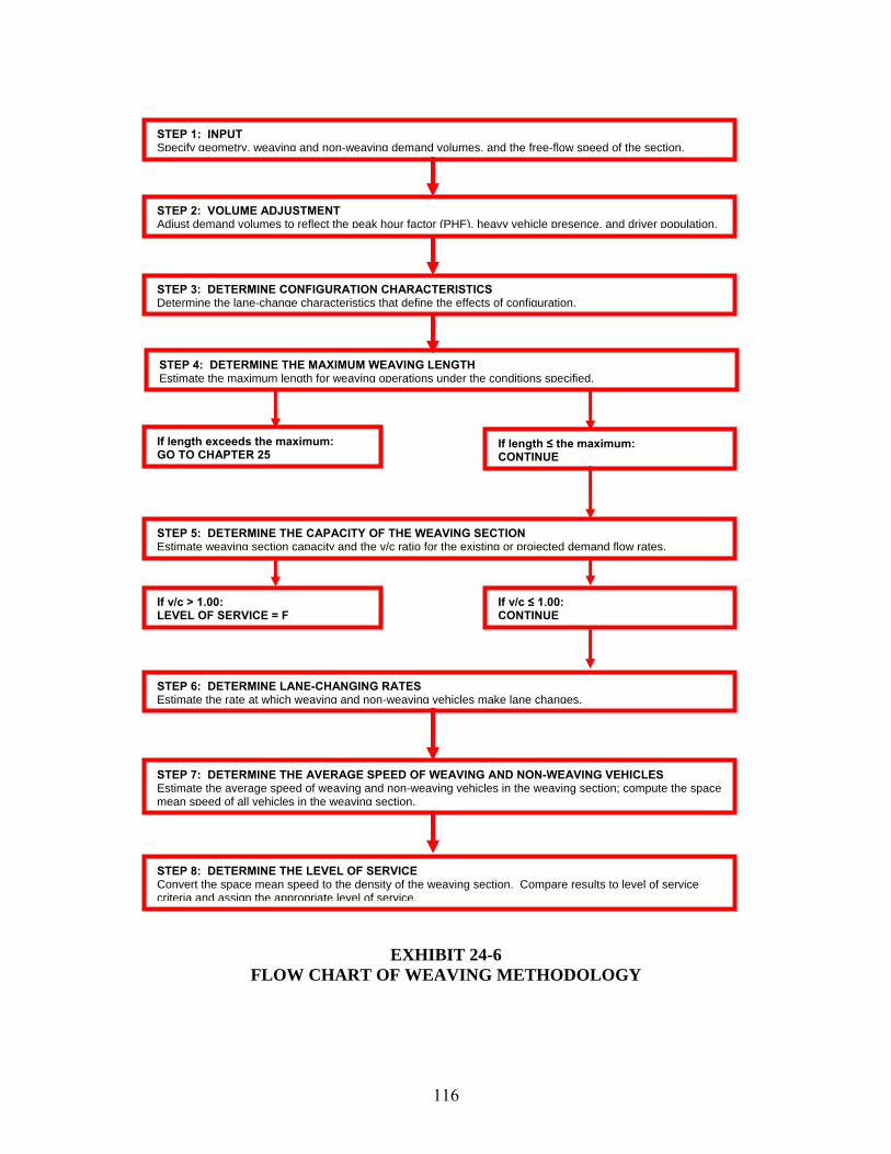
116
EXHIBIT 24-6
FLOW CHART OF WEAVING METHODOLOGY
STEP 1: INPUT Specify geometry, weaving and non-weaving demand volumes, and the free-flow speed of the section.
STEP 2: VOLUME ADJUSTMENT Adjust demand volumes to reflect the peak hour factor (PHF), heavy vehicle presence, and driver population.
STEP 3: DETERMINE CONFIGURATION CHARACTERISTICS Determine the lane-change characteristics that define the effects of configuration.
STEP 4: DETERMINE THE MAXIMUM WEAVING LENGTH Estimate the maximum length for weaving operations under the conditions specified.
If length exceeds the maximum: GO TO CHAPTER 25
If length ≤ the maximum: CONTINUE
STEP 5: DETERMINE THE CAPACITY OF THE WEAVING SECTION Estimate weaving section capacity and the v/c ratio for the existing or projected demand flow rates.
If v/c > 1.00: LEVEL OF SERVICE = F
If v/c ≤ 1.00: CONTINUE
STEP 6: DETERMINE LANE-CHANGING RATES Estimate the rate at which weaving and non-weaving vehicles make lane changes.
STEP 7: DETERMINE THE AVERAGE SPEED OF WEAVING AND NON-WEAVING VEHICLES Estimate the average speed of weaving and non-weaving vehicles in the weaving section; compute the space mean speed of all vehicles in the weaving section.
STEP 8: DETERMINE THE LEVEL OF SERVICE Convert the space mean speed to the density of the weaving section. Compare results to level of service criteria and assign the appropriate level of service.

117
EXHIBIT 24-7 WEAVING VARIABLES FOR ONE-SIDED WEAVING SECTIONS
Freeway Ramp
Freeway Ramp
vFF vRF
vFR vRR
Symbol Definition vFF freeway-to-freeway demand flow rate in the weaving section (pc/h) vRF ramp-to-freeway demand flow rate in the weaving section (pc/h) vFR freeway-to-ramp demand flow rate in the weaving section (pc/h) vRR ramp-to-ramp demand flow rate in the weaving section (pc/h) vW weaving demand flow rate in the weaving section (pc/h) vW = vRF + vFR vNW non-weaving demand flow rate in the weaving section (pc/h) vNW = vFF + vRR
v = total demand flow rate in the weaving section (pc/h) v = vW + vNW VR volume ratio: VR = vW/v N number of lanes within the weaving section NWL number of lanes from which a weaving maneuver may be made with one or no lane changes (See Exhibit 24-5) SW average speed of weaving vehicles within the weaving section (mi/h) SNW average speed of non-weaving vehicles within the weaving section (mi/h) S average speed of all vehicles within the weaving section (mi/h) FFS free-flow speed of the weaving section (mi/h) D average density of all vehicles within the weaving section (pc/mi/ln) W weaving intensity factor LS length of the weaving section (ft), based on short length definition of Exh 24-2 LCRF minimum number of lane changes that must be made by a single weaving
vehicle moving from the on-ramp to the freeway (See Exhibit 24-5) LCFR minimum number of lane changes that must be made by a single weaving
vehicle moving from the freeway to the ramp LCMIN minimum rate of lane changing that must exist for all weaving vehicles to successfully complete their weaving maneuvers (lc/h) LCMIN = (LCRF x vRF) + (LCFR x vFR) LCW total rate of lane changing by weaving vehicles within the weaving section (lc/h) LCNW total rate of lane changing by non-weaving vehicles within the weaving
section (lc/h) LCALL total lane-changing rate of all vehicles within the weaving section (lc/h) LCALL = LCW + LCNW

118
EXHIBIT 24-8 WEAVING VARIABLES FOR A TWO-SIDED WEAVING SECTION
Ramp
Freeway Freeway
Ramp
vRF vFF vRR vFR
All variables are defined as in Exhibit 24-7, except for the following variables related to flow designations and lane-changing variables. Symbol Definition vW total weaving demand flow rate within the weaving section (pc/h) vW = vRR vNW total non-weaving demand flow rate within the weaving section (pc/h) vNW = vFR + vRF + vFF LCRR minimum number of lane changes that must be made by one ramp-to-ramp
vehicle to complete a weaving maneuver. LCMIN minimum rate of lane changing that must exist for all weaving vehicles
to successfully complete their weaving maneuvers (lc/h) LCMIN = (LCRR x vRR)

119
• Models to predict the capacity of the weaving section under both ideal and prevailing conditions.
• A model to estimate the maximum length at which weaving operations can be said to
exist. The principal difference between one-sided and two-sided weaving sections is the relative positioning of the movements within the weaving section. In a two-sided weaving section, the ramp-to-freeway and freeway-to-ramp movements do not weave. In a one-sided section, they are the weaving movements. In a two-sided weaving section, the ramp-to-ramp vehicles must cross the path of freeway-to-freeway vehicles. Both could be taken to be weaving movements. In reality, the through freeway movement is not “weaving,” in that they need not change lanes and are generally not shifting lane position in response to desired exit leg. Thus, in two-sided weaving sections, only the ramp-to-ramp flow is considered to be “weaving.” Given this change in the way weaving flows are viewed, the lane-changing parameters must also reflect this. Thus, the minimum rate of lane-changing that weaving vehicles must maintain to successfully complete their desired maneuvers is also related only to the ramp-to-ramp movement. The definitions for flow all refer to demand flow rate. For future cases, forecasting techniques will generally produce a demand volume or flow rate. All algorithms of the methodology use demand expressed as flow rates in the peak 15 minutes of the design (or analysis) hour, in passenger car units. COMPUTATIONAL PROCEDURE Each of the major procedural steps noted in Exhibit 24-6 are discussed in greater detail in the sections which follow. Step 1 – Input The methodology for weaving sections is structured for operational analysis usage, i.e., given a known geometric design and traffic demand characteristics, the methodology is used to estimate the level of service that is expected to exist.
Design is generally conducted in terms of comparative analyses of various design proposals. This is a good approach, given that the range of widths, lengths, and configurations in any given case are restrained by a number of factors. The length is constrained by the location of crossing arteries that determine the location of interchanges and ramps. Width is constrained by the number of lanes on entry and exit legs, and usually involves no more than two choices. Configuration is also the result of the number of lanes on entry and exit legs and number of lanes within the section. Changing the configuration would involve adding a lane, usually to one of the entry or exit legs to create different linkages.

120
For any analysis, the full geometry of the weaving section must be fully defined. This includes number of lanes and lane widths, shoulder clearances, the details of entry and exit gore area designs, including markings, the existence and extent of barrier lines, and the length of the section. A sketch of the weaving section should be drawn with all appropriate dimensions shown.
Traffic demands are usually expressed as peak hour volumes under prevailing conditions.
If flow rates have been directly observed in the field, the flow rates for the worst 15 minutes in the peak hour may be substituted.
Step 2 – Volume Adjustment All algorithms use flow rates under equivalent ideal conditions as inputs. Thus, demand volumes or flow rates under prevailing conditions must be converted to their ideal equivalents using Equation 24-1: [24-1]
pHV
ii ffPHF
Vv
**=
where: vi = flow rate for flow “i” under ideal conditions (pc/h) Vi = hourly volume for flow “i” under prevailing conditions
(veh/h) PHF = peak hour factor fHV = adjustment factor for heavy-vehicle presence fp = adjustment factor for driver population subscript “i” definitions: FF = freeway-to-freeway FR = freeway-to-ramp RF = ramp-to-freeway RR = ramp-to-ramp W = weaving NW = non-weaving If flow rates (for a 15-minute period) have been provided as inputs, the PHF is taken to be 1.00 in this computation. Where hourly volumes are converted using a PHF (other than 1.00), there is an implicit assumption that all four component flows in the weaving section peak during the same 15-minute period of the hour. This is rarely true, and such an analysis represents a worst-case scenario. The adjustment factors fHV and fp are taken from Chapter 23 of this manual for basic freeway sections.

121
Once demand flow rates have been established, it may be convenient to construct a weaving diagram similar to those illustrated in Exhibits 24-7 (for one-sided weaving sections) and 24-8 (for two-sided weaving sections). Step 3 – Determine Configuration Characteristics There are several parameters, discussed previously, that numerically define the key configuration characteristics of the weaving section. In all cases, the following variables must be determined:
LCMIN = minimum hourly rate of successful lane changes required by weaving vehicles during the analysis period.
NWL = number of lanes from which weaving maneuvers may be made with either
one lane change or no lane changes; referred to as the number of weaving lanes.
The determination of these values depends upon whether the section under study is a one-sided or two-sided weaving section. One-Sided Weaving Sections The determination of key variables in one-sided weaving sections is illustrated in Exhibit 24-5. In one-sided weaving sections, the two weaving movements are the ramp-to-freeway and freeway-to-ramp flows. As shown in Exhibit 24-5, the following values are established:
LCRF = minimum number of lane-changes that must be made by one ramp-to-freeway vehicle to successfully execute the desired movement;
LCFR = minimum number of lane-changes that must be made by one freeway-to-
ramp vehicle to successfully execute the desired movement.
Then: [24-2]
( ) ( )FRFRRFRFMIN vLCvLCLC ** += where all terms are as previously defined. For one-sided weaving sections, the value of NWL is either “2” or “3.” The determination is made by a review of the geometric design and configuration of the weaving section, as shown in Exhibit 24-5.

122
Two-Sided Weaving Sections The determination of key variables in two-sided weaving sections is illustrated in Exhibit 24-4. The unique feature of two-sided weaving sections is that only the ramp-to-ramp flow is functionally “weaving.” From Exhibit 24-4, the following value is established:
LCRR = minimum number of lane-changes that must be made by one ramp-to-ramp vehicle to successfully execute the desired movement
Then: [24-3]
RRRR vLCLC *min = where all terms are as previously defined in Exhibit 24-4. For two-sided weaving sections, the value of NWL is “0” by definition. Step 4 – Determine the Maximum Weaving Length The concept of “maximum length” of a weaving section is an interesting one. Strictly defined, it is the length at which weaving turbulence no longer has an impact on operations within the section, or alternatively, on the capacity of the weaving section. Unfortunately, depending on the definition selected, the answers can be quite different. In fact, weaving turbulence will have an impact on operations (i.e. weaving and non-weaving vehicle speeds) for distances far in excess of those defined by when the capacity of the section is no longer affected by weaving. This methodology uses the latter definition. The selection is made on a logical basis. If longer lengths were treated as weaving sections, the methodology would produce a capacity for the weaving section that exceeds that of a basic freeway section with the same number of lanes and conditions. The following algorithm determines the length at which the capacity of the weaving section is the same as a basic freeway section with the same number of lanes: [24-4]
( )[ ] [ ]WLMAX NVRL *156615728 6.1 −+= Where LMAX is the maximum weaving section length (using the short-length definition), and other variables are as previously defined. The equation was derived by setting the per-lane capacity of a weaving section (with the prevailing conditions that exist) equal to the per-lane capacity of a basic freeway section (with the same prevailing conditions).

123
Obviously, as VR increases, it would be expected that the impact of weaving turbulence would extend further. All values of NWL are either “0” (two-sided weaving sections), “2” or “3” (one-sided weaving sections). Having more lanes from which easy weaving maneuvers can be made reduces lane-changing turbulence, which in turn means that the length at which turbulence affects capacity is reduced. The value of LMAX is used to determine whether continued analysis of the configuration as a weaving section is justified. The definition of LS is found in Exhibit 24-2.
• If LMAX ≥ LS, continue to Step 5
• If LMAX < LS, go to Chapter 25 of this manual If the section is “too long” to be considered a weaving section, then the analysis must be treated as isolated merge and diverge areas using the methodology presented in Chapter 25 for ramp junctions. Any distance between the junctions that falls outside of the merge or diverge influence areas (defined in Chapter 25) would be treated as a basic freeway section. Step 5 – Determine the Capacity of the Weaving Section The capacity of a weaving section can be controlled by one of two conditions:
• Breakdown of a weaving section is expected to occur when the average density of all vehicles in the section reaches 43 pc/mi/ln.
• Breakdown of a weaving section is expected to occur when the total weaving
demand flow rates exceeds the following:
2,400 pc/h for cases in which NWL = 2 3,500 pc/h for cases in which NWL = 3
The first expectation is based upon the criteria of Chapter 23 (Basic Freeway Sections), where freeway breakdown occurs at a density of 45 pc/mi/ln. Given the additional turbulence in a weaving section, breakdown is expected to occur at slightly lower densities. The second limit recognizes that there is a practical limit to how many vehicles can actually cross each other’s path without causing serious operational breakdowns. The existence of a third lane from which weaving movements can be easily made in effect spreads out the impacts of turbulence across section lanes, and allows for higher weaving flows. No limiting value on weaving flow rate is proposed for two-sided weaving sections (in which NWL = 0). The analysis of two-sided weaving sections is approximate using this methodology, and a density sufficient to cause a breakdown is generally at relatively low weaving flow rates in such cases.

124
Weaving Section Capacity Determined by Density The capacity of a weaving section, based upon reaching a density of 43 pc/mi/ln is estimated using the following algorithm: [24-5]
( )[ ] [ ] [ ]WLSIFLIWL NLVRcc *8.119*0765.012.438 6.1 +++−=
where: cIWL = capacity of the weaving section under ideal conditions per lane (pc/h/ln);
cIFL = capacity of a basic freeway section (with the same free-flow speed
as the weaving section) under ideal conditions per lane (pc/h/ln). All other variables are as previously defined in Exhibit 24-7. The model describes capacity of a weaving section in terms of the differential relative to the capacity of a basic freeway section with the same free-flow speed. Capacity decreases with an increase in the volume ratio (VR), which is logical. It also increases with increasing length. Also logical, it confirms that additional length adds capacity to a weaving section, all other variables being equal. It also increases with increasing NWL; this is logical as higher values disperse lane-changing turbulence across the lanes of the section. While it is arithmetically possible to get a result in which cIWL is greater than cIFL, this will never happen. The maximum length algorithm of Step 4 was found by setting cIWL= cIFL in this equation. Thus, if properly applied, such a result will not occur. The capacity of the weaving section under prevailing conditions is computed as follows: [24-6]
pHVIWLW ffNcc ***= where cW is the capacity of the weaving section under prevailing conditions in veh/h. As with all capacities, it is stated as a flow rate for a 15-minute period. Weaving Capacity Determined By Weaving Demand Flows The capacity of a weaving section, as controlled by the maximum weaving flow rates noted previously is found as: [24-7]
3500,3
2400,2
==
==
WLIW
WLIW
NforVR
c
NforVR
c

125
where cIW is the capacity of all lanes of the weaving section under ideal conditions, and all other variables are as previously defined. The capacity of the weaving section under prevailing conditions is computed as: [24-8]
pHVIWW ffcc **= where all terms are as previously defined. Final Capacity Determination The final capacity is the smallest of the two estimates given by equations [24-6] and [24-8]. The v/c ratio for the section can also be determined by dividing the total demand flow by the capacity: [24-9]
( )w
pHV
cffv
cv**
/ =
where all terms are as previously defined. Adjustment factors are used because the total demand flow, v, is stated for ideal conditions, while cW is stated for prevailing conditions. Level of Service F? If v/c > 1.00, demand exceeds capacity, and the section is expected to fail, i.e., have a level of service of F. If this occurs, the analysis stops, and level of service F is assigned. If v/c ≤ 1.00, continue the analysis to Step 6. Step 6 – Determine Lane-Changing Rates The equivalent hourly rate at which weaving and non-weaving vehicles make lane changes within the weaving section is a direct measure of turbulence. It is also a key determinant of speeds and densities which ultimately determine the existing or anticipated level of service. There are three types of lane changes that are made within a weaving section:
• Required lane changes made by weaving vehicles: These lane changes must be made to complete a weaving maneuver, and are restricted to the physical area of the weaving section. In Step 3, the rate at which such lane changes are made by weaving vehicles, LCMIN was determined.

126
• Optional lane changes made by weaving vehicles: These lane changes are not necessary to successfully weave. They involve weaving vehicles that choose to enter the weaving section in outer lanes of either the freeway or the ramp (assuming that is has more than one lane), and/or leave it in an outer lane. Such vehicles make additional lane changes beyond those absolutely required by their maneuver.
• Optional lane changes made by non-weaving vehicles: Non-weaving vehicles
may also make lane changes within the weaving section, but neither the configuration nor their desired origin and destination require such lane changes. Lane changes by non-weaving vehicles are always made on the option of the driver.
While LCMIN can be computed knowing the configuration and demand flow rates, additional optional lane changes made by both weaving and non-weaving vehicles must be estimated using regression-based models. Estimating the Total Lane-Changing Rate for Weaving Vehicles The model for predicting the total lane-change rate for weaving vehicles is of the form LCMIN plus an algorithm that predicts the additional optional lane change rate. These are combined, so that the total lane-changing rate for weaving vehicles, including both required and optional lane changes is: [24-10]
( ) ( )[ ]8.025.0 130039.0 IDNLLCLC SMINW +−+= where: LCW = equivalent hourly rate at which weaving vehicles make lane
changes within the weaving section (lc/h);
LCMIN = minimum equivalent hourly rate at which weaving vehicles must make lane changes within the weaving section to successfully complete all weaving maneuvers (lc/h);
LS = length of the weaving section, using the short length definition (ft); N = number of lanes within the weaving section; ID = interchange density.
The algorithm has several interesting characteristics. The term “LS – 300” implies that in weaving sections of 300 ft (or shorter), weaving vehicles only make necessary lane changes, i.e., LCW = LCMIN. While shorter weaving sections would be an aberration, in using this algorithm, a length that is less than 300 ft must be entered as “300.”

127
This is also the first model that is NOT a free-flow speed estimator that uses the interchange density, ID. The algorithm uses the term “1 + ID” because the value of ID may be either more or less than 1.00, and the power term would not act consistently on the result. In determining the interchange density for a weaving section, a distance of 3 miles upstream and 3 miles downstream of the midpoint of the weaving section should be used. The number of interchanges located within the 6-mile area is counted and divided by 6 to determine ID. The subject weaving section should be counted as one interchange. For additional discussion of interchange density and its measurement, consult Chapter 23 of this manual. The basic sensitivities of this model are reasonable. Weaving vehicle lane-changing increases with increasing length and width of the weaving section. A longer, wider weaving section simply provides more opportunities for weaving vehicles to execute lane changes. Lane-changing also increases with interchange density. This is also logical, as higher interchange densities mean that there are more reasons for vehicles to make optional lane changes based upon their entry or exit at a nearby interchange. Estimating the Lane-Changing Rate for Non-Weaving Vehicles No non-weaving vehicle must make a lane change within the confines of a weaving section. All non-weaving vehicle lane-changes are, therefore, of the optional variety. These are more difficult to predict than weaving lane changes, as the motivation for optional lane changes vary widely, and may not always be obvious. Lane changes may be made to avoid the turbulence of the weaving section, to be better positioned for a subsequent maneuver, or simply to achieve a higher speed. The research leading to the development of this methodology [1] revealed several discontinuities in the lane-changing behavior of non-weaving vehicles within weaving sections. To identify the areas of discontinuity, it was necessary to develop a non-weaving vehicle index, as follows: [24-11]
000,10** NWS
NWvIDL
I =
where INW is the index, and all other variables are as previously defined. The index is a relative measure of parameters that might induce unusually large rates of non-weaving vehicle lane changing. Large non-weaving flow rates, interchange densities, and length appear to combine to produce unusually high lane-change rates, thereby introducing some discontinuity into the model. Two models are used to predict the rate at which non-weaving vehicles change lanes in weaving sections: [24-12]
( ) ( ) ( )NLvLC SNWNW *6.192*542.0*206.01 −+=

128
[24-13]
( )000,2223.0135,22 −+= NWNW vLC where LCNW1 and LCNW2 are two estimates of the rate at which non-weaving lane changes are made (lc/h), and all other variables are as previously defined. Equation [24-12] covers the majority of situations. Non-weaving lane changing increases with increasing non-weaving flow and section length, both of which are logical. Less expected is the decrease in non-weaving lane changing with increasing width. This trend is statistically strong, and most likely indicates more pre-segregation of flows in wider sections. Arithmetically, Equation [24-12] can produce a negative result. Thus, the minimum value must be externally set at “0.” Equation [24-13] is significantly discontinuous with Equation [24-12], and applies to a small number of cases in which the combination of high non-weaving demand flow, interchange density, and section length is such that extraordinary non-weaving lane-changing rates prevail. The index is used to define which equation applies. Because of the discontinuity between the two, there is also a range in which the two values must be interpolated. The non-weaving lane-changing rate is: [24-14]
( ) ⎟⎠⎞
⎜⎝⎛ −
−+=
>>
=≥
=≤
6501300
*
:19501300
:1950
:300,1
121
2
1
NWNWNWNWNW
W
NWNW
NW
NWNW
NW
ILCLCLCLC
IIf
LCLCIIf
LCLCIIf
The interpolation process does not work if LCNW1 > LCNW2. Such a result will not normally occur, as long as the analysis is within the maximum weaving length criteria estimated in Step 4. If such a result occurs, and weaving length is appropriate, the result for LCNW2 is used to estimate LCNW.

129
Total Lane Changing Rate The total lane-changing rate of all vehicles in the weaving section is computed as: [24-15]
NWWALL LCLCLC += where all variables are as previously defined. Step 7 -- Determine the Average Speeds of Weaving and Non-Weaving Vehicles The heart of the analysis methodology for weaving sections is the estimation of average speeds of weaving and non-weaving vehicles. They are estimated separately because they are affected by different factors, and they can be significantly different from each other. The speeds of weaving and non-weaving vehicles will be combined to find a space mean speed for all vehicles. This is converted to a density, which will determine the level of service. Average Speed of Weaving Vehicles The algorithm for prediction of average weaving speed may be generally stated as: [24-16]
⎟⎠⎞
⎜⎝⎛
+−
+=WSSSS MINMAX
MINW 1
where: SW = average speed of weaving vehicles within the weaving section
(mi/h) SMIN = minimum average speed expected in a weaving section (mi/h) SMAX = maximum average speed expected in a weaving section (mi/h) W = weaving intensity factor The form of the model is logical, and constrains results to a reasonable range, defined by minimum and maximum speed expectations. The term “1 + W” accommodates a weaving intensity factor that may be more or less than 1.0. For this methodology, the minimum expected speed is taken to be 15 mi/h. The maximum speed is set equal to the free-flow speed, FFS. As is the case in all analyses, the free-flow speed is best measured in the field, either on the subject facility, or a similar facility. When measured, the FFS should be observed within the weaving section.

130
Where the FFS must be estimated, the model described in Chapter 23 of this manual for basic freeway sections is used, with the following recommended modification: the adjustment factor for the number of lanes on the freeway should NOT be applied. The average speed of weaving vehicles within the weaving section is estimated as follows: [24-17]
⎟⎠⎞
⎜⎝⎛
+−
+=W
FFSSW 11515
789.0
*226.0 ⎟⎟⎠
⎞⎜⎜⎝
⎛=
S
ALL
LLCW
where all terms are as previously defined. Note that “weaving intensity” is based on the total lane-changing rate within the weaving section. In fact, the factor is based upon the hourly rate of lane-changes per foot of weaving section length. This might be thought of as a measure of the density of lane changes. It should also be noted that the lane-change rate is itself dependent upon many demand and physical factors related to the design of the section. Average Speed of Non-Weaving Vehicles The average speed of non-weaving vehicles in a weaving section is estimated using the following model: [24-18]
( ) ( )NvLCFFSS MINNW *0048.0*0072.0 −−=
where all terms are as previously defined. The model treats non-weaving speed as a reduction from the free-flow speed. As might be expected, the speed is reduced as v/N increases. More interesting is the appearance of LCMIN in the equation. LCMIN is a measure of minimal weaving turbulence, assuming that weaving vehicles make only necessary lane changes. It is dependent upon the configuration of the weaving section, and the weaving demand flow rates. The model predicts that non-weaving vehicle speeds will decrease with increasing flow per lane, and with increasing weaving turbulence, in this case measured by the variable LCMIN. Average Speed of All Vehicles The space mean speed of all vehicles in the weaving section is computed as follows: [24-19]
⎟⎟⎠
⎞⎜⎜⎝
⎛+⎟⎟
⎠
⎞⎜⎜⎝
⎛+
=
NW
NW
w
w
NWW
Sv
Sv
vvS

131
where all terms are as previously defined. Step 8 – Determine the Level of Service The level of service of a weaving section, as in all freeway analysis, is related to the density in the section. Criteria are shown in Exhibit 24 -9.
EXHIBIT 24-9 LEVEL OF SERVICE CRITERIA FOR WEAVING SECTIONS
Density (pc/mi/ln)
LOS
Freeway Weaving Sections
Weaving Sections on C-D Roadways or Multilane Highways
A 0 – 10 0 – 12 B >10 – 20 > 12 – 24 C > 20 – 28 > 24 – 32 D > 28 – 35 > 32 – 36 E > 35 > 36 F v/c > 1.00
Exhibit 24-9 provides level of service criteria for weaving sections on freeways, collector-distributor roadways, and multilane highways. The methodology was developed for freeway weaving sections, although an isolated collector – distributor roadway was included in its development. As in past editions of this manual, application of the weaving section methodology to weaving sections on uninterrupted sections of multilane surface facilities is permitted, although its use in such cases is approximate. The boundary between stable and unstable flow – the boundary between levels of service E and F – is based solely upon the v/c ratio for the section, as described in Step 5 of the methodology. The threshold densities for other levels of service were set relative to the criteria for basic freeway sections (or multilane highways). In general, density thresholds in weaving sections are somewhat higher than those for similar basic freeway sections (or multilane highways). It is believed that drivers will tolerate higher densities in an area where lane-changing turbulence is expected than on basic sections. To apply density criteria, the average speed of all vehicles, computed in Step 7, must be converted to a density: [24-20]
SNvD /
=
where D is the density in pc/mi/ln, and all other variables are as previously defined.

132
SERVICE FLOW RATES AND VOLUMES As in previous chapters, a service flow rate (SFi) is the maximum rate of flow that can be sustained under prevailing roadway, traffic, and control conditions while maintaining a level of service i. Thus, for the five levels of service, A-E, there is a service flow rate. For weaving sections, as is the case for basic freeway sections, the service flow rate for level of service E is the capacity of the weaving section, cW. Service flow rates are affected by virtually all factors involved in weaving sections, including component demand volumes, heavy vehicle presence, driver population, the length, width, and configuration of the weaving section, free-flow speeds, the interchange density, and other variables that have been discussed. Service flow rates can be established by specifying a demand pattern (% distribution among the component flows in the weaving section), traffic factors such as % heavy vehicles, and the complete geometry of the section. The total demand is then incrementally raised until the threshold density for a particular level of service is attained. For freeway weaving sections, service flow rates for various levels of service under ideal conditions (SFIi) are set when the following densities are achieved: SFIA D = 10 pc/mi/ln SFIB D = 20 pc/mi/ln SFIC D = 28 pc/mi/ln SFID D = 35 pc/mi/ln SFIE = cW An ideal service flow rate is converted to reflect prevailing conditions as follows: [24-21]
pHVii ffSFISF **= where all terms are as previously defined. A service volume (SVi) is the maximum full-hour volume that can be sustained under prevailing roadway, traffic, and control conditions while not exceeding the threshold density for a particular level of service within the worst 15 minutes of the hour. A service volume is easily found using the service flow rate and peak hour factor: [24-22]
PHFSFSV ii *= The example problems include an illustration of how service flow rates and service volumes can be generated for a particular case.

133
MULTIPLE WEAVING SECTIONS When a series of closely-spaced merge and diverge areas create overlapping weaving movements (between different merge-diverge pairs) that share the same section of a roadway, a multiple weaving section is created. In earlier editions of this manual, a specific application of the weaving methodology for two-segment multiple weaving sections was included. While it was a logical extension of the methodology, it did not address cases in which three or more sets of weaving movements overlapped, and was not well-supported by field data. Multiple weaving sections should be segregated into separate merge, diverge, and simple weaving sections, with each section appropriately analyzed using the methodologies of this chapter, or of Chapter 25 (for merge and diverge areas). Chapter 22 contains information relative to the process of identifying appropriate sections for analysis. COLLECTOR-DISTRIBUTOR ROADWAYS A common design practice often results in weaving movements that occur on collector-distributor roadways that are part of a freeway interchange. The methodology of this chapter may be approximately applied to such cases, although the free-flow speed used must be appropriate to the collector-distributor roadway. It would have to be measured on an existing or similar C-D roadway, as the predictive methodology for FFS given in Chapter 23 does not apply to C-D roadways. It is less clear that the LOS criteria of Exhibit 24-9 are appropriate. Many C-D roadways operate at lower speeds and higher densities than on basic sections. The criteria of Exhibit 24-9 may produce an inappropriately negative view of operations on the C-D roadway. MULTILANE HIGHWAYS There are weaving sections that occur on surface multilane highways. As long as such sections are sufficiently far away from signalized intersections – so that platoon movements are not an issue – the methodology of this chapter may be approximately applied. ARTERIAL WEAVING The methodology of this chapter does not apply to weaving sections on arterials. Arterial weaving is heavily affected by the proximity and timing of signals along the arterial. At the present time, there are no generally accepted methodologies for analysis of weaving movements on arterials.

134
III. APPLICATIONS The methodology of this chapter is most easily applied in the operational analysis mode. In this application, all weaving section demands and geometric elements are known, and the output of analysis is the expected level of service. Secondary outputs include the average speed of component flows, the overall density in the section, and measures of lane-changing activity. In design applications, the desired output is the length, width, and configuration of a weaving section that will sustain a target level of service for given demand flows. This application is best accomplished by trial-and-error operational analyses on a small section of candidate designs. As noted previously, there generally is not a great deal of flexibility in establishing the length and width of a weaving section, and only limited flexibility in potential configurations. Planning applications generally have the same desired outputs as design applications: the geometric design of a weaving section that can sustain a target level of service for given demand flows. In general, however, in the planning stage, demand flows are given as average annual daily traffic estimates (AADT), which must be converted to directional design hour volumes (DDHV). A number of variables may be unknown, and may be replaced by default values. As the methodology requires the specification of many variables, the analyst has four sources of input data that can be used:
1. Default values found elsewhere in this manual. 2. Estimates and locally-derived default values developed by the analyst or a local
transportation agency. 3. Values derived from field measurements and observations. 4. Demand values obtained from traffic forecasts.
A variety of applications are illustrated in the example problems of the next section.

135
IV. EXAMPLE PROBLEMS
Problem Description Application 1 Determining LOS of a major weaving section Operational analysis 2 Determining LOS of a ramp-weave section Operational analysis 3 Determining LOS of a two-sided weaving section Operational analysis 4 Design a major weaving section for a desired LOS Design 5 Construct a service volume table for a weaving
section Service volumes

136
Example Problem 1 The Weaving Section The subject of this operational analysis is a major weaving section on an urban freeway, as shown in Exhibit 24-10.
Exhibit 24-10
Weaving Section for Example Problem 1 The Questions What are the level of service and capacity of the weaving section with the design and peak hour demands as shown? The Facts In addition to the information given in Exhibit 24-10, the following characteristics of the weaving section are known: PHF: 0.91 (all movements) Heavy Vehicles: 10% Trucks; 0% RV’s (all movements) Driver Population: Regular commuters FFS: 65 mi/h cIFL: 2,350 pc/h/ln (for FFS = 65 mi/h) ID: 0.8 interchanges/mi Terrain: Level
Freeway Freeway
Ramp Ramp
LS = 1,500 ft
VFF = 1,815 veh/h VRF = 1,037 veh/h VFR = 692 veh/h VRR = 1,297 veh/h V = 4,841 veh/h

137
Comments Chapter 23, “Basic Freeway Sections” must be consulted to find appropriate values of fHV and fp. Outline of Solution All input parameters have been specified, so default values are not needed. Demand volumes are given in veh/h under prevailing conditions, and must be converted to pc/h under equivalent ideal conditions. The length of the section must be compared to the maximum length for weaving analysis to determine whether or not a weaving analysis is appropriate. The capacity of the weaving section is estimated and compared to the total demand flow to determine whether level of service F exists. Lane-changing rates are estimated to allow speed estimates to be made for weaving and non-weaving vehicles. An average overall speed and density are computed, and an appropriate level of service is assigned based upon the predicted density. Computational Steps Specify Input Data
See Exhibit 24-10 and example statement.
Volume Adjustment
From Ch 23, ET = 1.5; fp = 1
357.055861995/586,535911995
/591,314972094/995,11197798
/497,11*952.0*91.0
1297
/197,11*952.0*91.0
1037
/7981*952.0*91.0
692
/094,21*952.0*91.0
1815
952.0)15.1(10.01
1)1()1(1
1
===+=
=+==+=
==
==
==
==
=−+
=−+−+
=
VRhpcv
hpcvhpcv
hpcv
hpcv
hpcv
hpcv
EPEPf
NW
W
RR
RF
FR
FF
RRTTHV
Configuration Characteristics
The configuration is examined, as shown below, to determine the values of LCRF, LCFR, and NWL. LCMIN may then be computed:

138
LCRF = 0 LCFR = 1 NWL = 3
hlcvLCvLCLC FRFRRFRFMIN /798)798*1()1197*0()*()*( =+=+=
Maximum Weaving Length
( )[ ] [ ]( )[ ] [ ]
AnalysisContinueftftL
NVRL
MAX
WLMAX
1500639,43*1566357.015728
1566157286.1
6.1
>=−+=
−+=
Capacity of the Weaving Section
Capacity controlled by density: ( )[ ] [ ] [ ]( )[ ] [ ] [ ]
hvehffNcchpcc
NLVRcc
pHVIWLW
IWL
WLSIFLIWL
/038,81*952.0*4*2110***ln//110,23*8.1191500*0765.0357.012.4382350
*8.119*0765.012.4387.1
6.1
====+++−=
+++−=
Capacity controlled by maximum weaving flow rate:
hvehffcchpcVRc
PHVIWW
IW
/333,91*952.0*9804**/804,9357.0/3500/3500
======
Controlling cW = 8,038 veh/h v/c =5586*0.952*1/8038 = 0.662 (Not LOS F, continue)
Lane-Changing Rates
For weaving vehicles: ( ) ( )[ ]
( ) ( )[ ] hlcLC
IDNLLCLC
W
SMINW
/144,18.014300150039.0799
130039.08.25.0
8.025.0
=+−+=
+−+=
For non-weaving vehicles:
( ) ( )( ) ( ) ( )( ) ( ) ( ) hlcLC
NLvLCvIDLI
NW
SNWNW
NWSNW
/7824*6.1921500*542.03592*206.0*6.192*542.0*206.0
1300431000,10/3591*8.0*1500000,10/**
=−+=−+=
<===
Total lane-change rate:
hlcLCLCLC NWWALL /926,17821144 =+=+=
Freeway Freeway
Ramp Ramp
LS = 1,500 ft

139
Speeds Weaving intensity factor:
( ) 275.015001926*226.0*226.0
789.0789.0
==⎟⎠⎞⎜
⎝⎛=
S
ALLL
LCW
Average speed of weaving vehicles:
hmiW
FFSSW /2.54275.01156515
11515 =⎟
⎠⎞
⎜⎝⎛+−
+=⎟⎠⎞
⎜⎝⎛
+−
+=
Average speed of non-weaving vehicles: ( ) ( )( ) ( ) hmiS
NvLCFFSS
NW
MINNW
/5.524/5586*0048.0799*0072.00.65/*0048.0*0072.0
=−−=−−=
Average speed of all vehicles:
hmi
Sv
Sv
vvS
NW
NW
W
W
NWW /1.53
5.523592
2.541996
35921996=
⎟⎠⎞
⎜⎝⎛+⎟
⎠⎞
⎜⎝⎛
+=
⎟⎟⎠
⎞⎜⎜⎝
⎛+⎟⎟
⎠
⎞⎜⎜⎝
⎛+
=
Density and Level of Service
Density: ( ) ( )
ln//3.261.534
5586mipc
SN
vD ===
Level of service (Exhibit 24-9): Level of service = C
Discussion As indicated by the results, this section operates at LOS C, with an average speed of 53.1 mi/h for all vehicles. Weaving vehicles travel a bit faster than non-weaving vehicles primarily because the configuration favors weaving vehicles. The difference, however, is small. With a v/c ratio of 0.662, the demand flow rate is considerably less than the capacity of 8,038 veh/h. Demand can grow significantly without reaching the capacity of the section.

140
Example Problem 2 The Weaving Section The weaving section that is the subject of this operational analysis is the one-sided ramp-weave section shown in Exhibit 24-11 below.
Exhibit 24-11
Weaving Section for Example Problem 2 The Questions What is the capacity of this weaving section, and at what LOS will it operate under the given demand volumes? The Facts In addition to the information in Exhibit 24-11, the following facts are known about the weaving section: PHF: 1.00 (demands given as flow rates) Heavy Vehicles: 0% Trucks; 0% RV’s (demands given as pc) Driver Population: Regular commuters FFS: 75 mi/h cIFL: 2,400 pc/h/ln (for FFS = 75 mi/h) ID: 1 interchange/mi Terrain: Level Comments Because the demand flows have been specified in pc/h under equivalent ideal conditions, Chapter 23 does not have to be consulted to obtain appropriate adjustment factors. Outline of Solution Because demand flows are already in their converted form – pc/h under equivalent ideal conditions – several computational steps are now trivial. Key lane-changing
LS = 1,000 ft
Freeway Ramp
Freeway Ramp
vFF = 4,000 pc/h vRF = 600 pc/h V = 5,000 pc/h vFR = 300 pc/h vRR = 100 pc/h
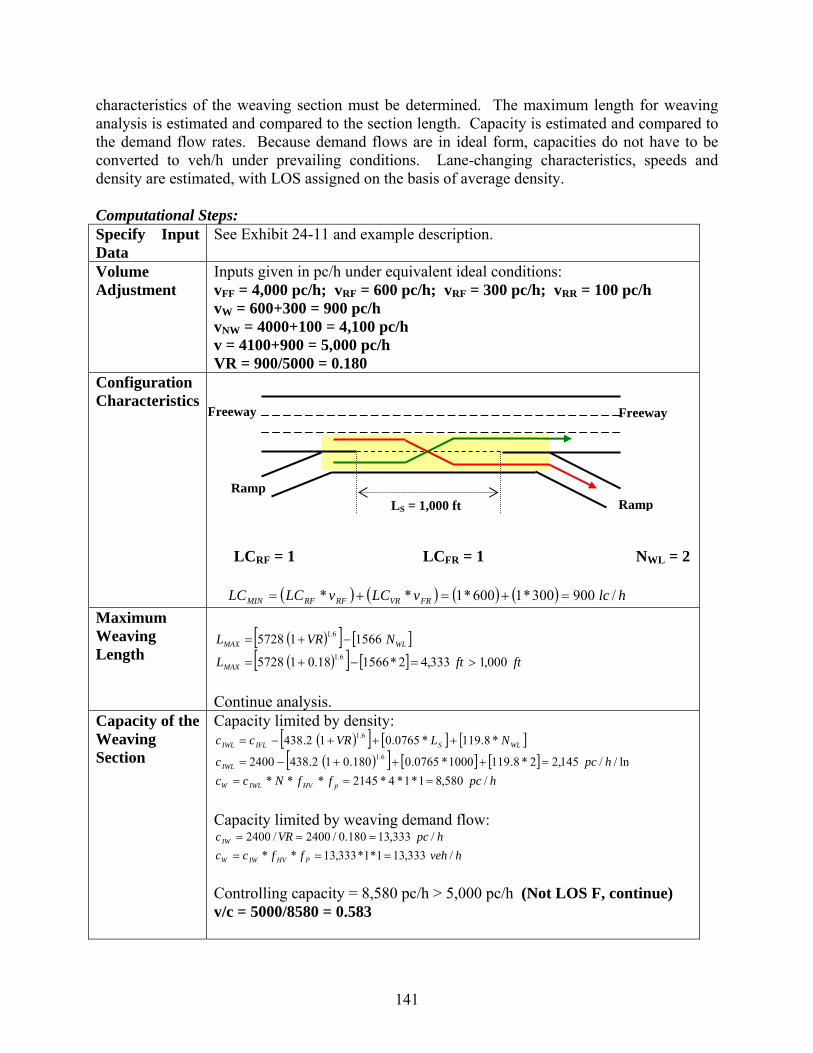
141
characteristics of the weaving section must be determined. The maximum length for weaving analysis is estimated and compared to the section length. Capacity is estimated and compared to the demand flow rates. Because demand flows are in ideal form, capacities do not have to be converted to veh/h under prevailing conditions. Lane-changing characteristics, speeds and density are estimated, with LOS assigned on the basis of average density. Computational Steps: Specify Input Data
See Exhibit 24-11 and example description.
Volume Adjustment
Inputs given in pc/h under equivalent ideal conditions: vFF = 4,000 pc/h; vRF = 600 pc/h; vRF = 300 pc/h; vRR = 100 pc/h vW = 600+300 = 900 pc/h vNW = 4000+100 = 4,100 pc/h v = 4100+900 = 5,000 pc/h VR = 900/5000 = 0.180
Configuration Characteristics
LCRF = 1 LCFR = 1 NWL = 2
( ) ( ) ( ) ( ) hlcvLCvLCLC FRVRRFRFMIN /900300*1600*1** =+=+= Maximum Weaving Length
( )[ ] [ ]( )[ ] [ ] ftftL
NVRL
MAX
WLMAX
000,1333,42*156618.015728
1566157286.1
6.1
>=−+=
−+=
Continue analysis. Capacity of the Weaving Section
Capacity limited by density: ( )[ ] [ ] [ ]( )[ ] [ ] [ ]
hpcffNcchpcc
NLVRcc
pHVIWLW
IWL
WLSIFLIWL
/580,81*1*4*2145***ln//145,22*8.1191000*0765.0180.012.4382400
*8.119*0765.012.4386.1
6.1
====+++−=
+++−=
Capacity limited by weaving demand flow:
hvehffcchpcVRc
PHVIWW
IW
/333,131*1*333,13**/333,13180.0/2400/2400
======
Controlling capacity = 8,580 pc/h > 5,000 pc/h (Not LOS F, continue) v/c = 5000/8580 = 0.583
Freeway Ramp LS = 1,000 ft
Freeway Ramp

142
Lane-Changing Rates
For weaving vehicles: ( ) ( )[ ]
( ) ( )[ ] hlcLC
IDNLLCLC
W
SMINW
/187,1114300100039.0900
130039.08.25.0
8.025.0
=+−+=
+−+=
For non-weaving vehicles:
( ) ( )( ) ( ) ( )( ) ( ) ( ) hlcLC
NLvLCvIDLI
NW
SNWNW
NWSNW
/6164*6.1921000*542.04100*206.0*6.192*542.0*206.0
1300410000,10/4100*1*1000000,10/**
=−+=−+=
<===
For all vehicles:
hlcLCLCLC NWWALL /803,16161187 =+=+= Speeds For weaving vehicles:
( ) 400.010002072*226.0*226.0
789.0789.0
==⎟⎠⎞⎜
⎝⎛=
S
ALLL
LCW
hmiW
FFSSW /1.59400.01157515
11515 =⎟
⎠⎞
⎜⎝⎛
+−
+=⎟⎠⎞
⎜⎝⎛
+−
+=
For non-weaving vehicles:
( ) ( )( ) ( ) hmiS
NvLCFFSS
NW
MINNW
/5.624/5000*0048.0900*0072.00.75/*0048.0*0072.0
=−−=−−=
For all vehicles:
hmi
Sv
Sv
vvS
NW
NW
W
W
NWW /9.61
5.624100
1.59900
4100900==
⎟⎠⎞
⎜⎝⎛+⎟
⎠⎞
⎜⎝⎛
+=
⎟⎟⎠
⎞⎜⎜⎝
⎛+⎟⎟
⎠
⎞⎜⎜⎝
⎛+
=
Density and LOS
Density: ( ) ( )
ln//2.206.614
5000mipc
SN
vD ===
Level of service (Exhibit 24-9): Level of service = C
Discussion The section operates at LOS C – but very close to the LOS B boundary (20 pc/mi/ln). Weaving and non-weaving average speeds are relatively high, and the demand flow of 5,000 pc/h is well below the capacity of 8,580 pc/h, allowing for some demand growth. Weaving vehicles travel somewhat slower than non-weaving vehicles. This is common in ramp-weave sections, where the vast majority of non-weaving vehicles are freeway-to-freeway.

143
Example Problem 3 The Weaving Section The two-sided weaving section that is the subject of this example is shown in Exhibit 24-12 below.
Exhibit 24-12
Weaving Section for Example Problem 3 The Facts In addition to the information given in Exhibit 24-12, the following information is known: PHF: 0.94 (all movements) Heavy Vehicles: 15% Trucks; 0% RV’s (all movements) Driver Population: Regular commuters FFS: 60 mi/h cIFL: 2,300 pc/h/ln (for FFS = 60 mi/h) ID: 2 interchanges/mi Terrain: Rolling
Freeway Freeway
Ramp
LS = 750 ft Ramp
VRF = 100 veh/h VFF = 3,500 veh/h V = 4,150 veh/h VRR = 300 veh/h VFR = 250 veh/h

144
Comments In this problem, we are dealing with a two-sided weaving section, which changes some of the basic definitions. The weaving volume only includes the ramp-to-ramp flow. While the freeway-to-freeway flow is technically weaving, their operation through the section is more like non-weaving vehicles, as they are not involved in a ramp movement. This section is in a busy corridor, with a high interchange density and relatively low free-flow speed. Outline of Solution Solution steps are the same as in Example Problems 1 and 2, but are modified to reflect the reality of the two-sided weave. Component volumes will be converted to pc/h under equivalent ideal conditions, and key demand parameters will be computed. A maximum weaving length will be computed to confirm that a weaving analysis is appropriate. Capacity will be determined to see if LOS F is expected. If not, lane-changing, speed, and density parameters will be estimated, and a level of service determined on the basis of density criteria. Computational Steps: Specify Input Data
See Exhibit 24-12 and supporting data.
Volume Adjustment
From Chapter 23, for Rolling Terrain: ET = 2.5; ER = 2.0; fp = 1.00
072.05410391/410,53915019
/019,51303264563/391
/3911*816.0*94.0
300
/1301*816.0*94.0
100
/3261*816.0*94.0
250
/563,41*816.0*94.0
3500
816.0)15.2(15.01
1)1()1(1
1
===+=
=++=++===
==
==
==
==
=−+
=−+−+
=
VRhpcv
hpcvvvvhpcvv
hpcv
hpcv
hpcv
hpcv
EPEPf
RFFRFFNW
RRW
RR
RF
FR
FF
RRTTHV
Configuration Characteristics
LCRR = 2 NW = 0 (by definition)
Freeway Freeway
Ramp
LS = 750 ft Ramp

145
( ) ( ) hlcvLCLC RRRRMIN /782391*2* ===
Maximum Weaving Length
( )[ ] [ ]( )[ ] [ ] ftftL
NVRL
MAX
WLMAX
750401,60*1566072.015728
1566157286.1
6.1
>=−+=
−+=
Continue analysis. Capacity of the Weaving Section
In a 2-sided weaving section, only a density-based capacity can be applied:
( )[ ] [ ] [ ]( )[ ] [ ] [ ]
965.04573/1*816.0*5410/
/573,41*816.0*3*1868***ln//868,10*8.119750*0765.0072.012.4382300
*8.119*0765.012.4386.1
6.1
==
====+++−=
+++−=
cv
hvehffNcchpcc
NLVRcc
pHVIWLW
IWL
WLSIFLIWL
Continue analysis – NOT LOS F. Lane-Changing Parameters
For weaving vehicles: ( ) ( )[ ]
( ) ( )[ ] hlcLC
IDNLLCLC
W
SMINW
/96121330075039.0782
130039.08.25.0
8.025.0
=+−+=
+−+=
For non-weaving vehicles:
( ) ( )( ) ( ) ( )( ) ( ) ( ) hlcLC
NLvLCvIDLI
NW
SNWNW
NWSNW
/8633*6.192750*542.05019*206.0*6.192*542.0*206.0
1300753000,10/5019*2*750000,10/**
=−+=−+=
<===
For all vehicles:
hlcLCLCLC NWWALL /824,1863961 =+=+= Speeds For weaving vehicles:
( ) 456.07501824*226.0*226.0
789.0789.0
==⎟⎠⎞⎜
⎝⎛=
S
ALLL
LCW
hmiW
FFSSW /9.45456.01156015
11515 =⎟
⎠⎞
⎜⎝⎛
+−
+=⎟⎠⎞
⎜⎝⎛
+−
+=
For non-weaving vehicles:
( ) ( )( ) ( ) hmiS
NvLCFFSS
NW
MINNW
/7.453/5410*0048.0782*0072.00.60/*0048.0*0072.0
=−−=−−=
For all vehicles:
hmi
Sv
Sv
vvS
NW
NW
W
W
NWW /7.45
7.455019
9.45391
5019391==
⎟⎠⎞
⎜⎝⎛+⎟
⎠⎞
⎜⎝⎛
+=
⎟⎟⎠
⎞⎜⎜⎝
⎛+⎟⎟
⎠
⎞⎜⎜⎝
⎛+
=
Density and LOS
ln//5.397.45
3/5410/ mipcSNvD ===
Level of service = E (Exhibit 24-9)

146
Discussion This two-sided weaving section is operating at LOS E, not far from the LOS E/F boundary. The v/c ratio is 0.965. The major problem is the 300 veh/h crossing the freeway from ramp-to-ramp. Two-sided weaving sections do not operate well with such large numbers of ramp-to-ramp vehicles. If this were just a basic freeway section, the per-lane flow rate of 5410/3 = 1,803 pc/h/ln would not be considered excessive, and would present a better LOS.

147
Example Problem 4 The Weaving Section A weaving section is to be designed between two major junctions in which two urban freeways join then separate. The situation is shown in Exhibit 24-13 below. Entry and exit legs have the number of lanes shown. The maximum length of the weaving section is 1,000 ft, and the free-flow speed of all legs is 75 mi/h. All demand flows are shown as flow rates under equivalent ideal conditions.
Exhibit 24-13
Weaving Section for Example Problem 4 The Question What design would be appropriate to deliver LOS C for the demand flow rates shown? The Facts In addition to the information given in Exhibit 24-13, the following facts are known concerning this weaving section: PHF: 1.00 (all demands stated as flow rates in pc/h) Heavy Vehicles: 0% Trucks; 0% RV’s (all demands in pc/h) Driver Population: Regular commuters FFS: 75 mi/h cIFL: 2,400 pc/h/ln (for FFS = 75 mi/h) ID: 1 interchanges/mi Terrain: Level
Ramp
FreewayFreeway
L (max) = 1,000 ft
Ramp
vFF = 2,000 pc/h vRF = 1,500 pc/h vFR = 1,450 pc/h vRR = 2,000 pc/h v = 6,950 pc/h

148
Comments As is the case in any weaving section design, there are considerable constraints imposed. The problem states that the maximum length is 1,000 ft, no doubt limited by location issues for the merge and diverge areas. It is probably not worth investigating shorter lengths, and the maximum should be assumed for all trial designs. The simplest design merely connects entering lanes with exit lanes in a straightforward manner, producing a section of 5 lanes. A section with 4 lanes could be considered by merging two lanes at the entry gore and separating it into two again at the exit gore. In any event, the design is limited to a section of 4 or 5 lanes. No other widths would work without major additions to input and output legs. The configuration cannot be changed without adding a lane to at least one of the entry and/or exit legs. Thus, the initial trial will be at a length of 1,000 ft, with the five entry lanes connected directly to the five exit lanes, with no changes to the exit or entry leg designs. If this does not produce an acceptable operation, changes will be considered. While the problem clearly states that all legs are freeways, no feasible configuration produces a two-sided weaving section. Thus, to fit within the one-sided analysis methodology, the right-side entry and exit legs will be classified as the “ramps” in the computational analysis. Computational Steps (1): Specify Input Data
See Exhibit 24-13 and supporting data.
Volume Adjustment
All demands are given as peak flow rates under equivalent ideal conditions. Thus, no conversions are needed:
424.06950/2950/950,640002950
/000,420002000/950,214501500
/000,2/500,1/450,1/000,2
===+=
=+==+=
====
VRhpcv
hpcvhpcv
hpcvhpcvhpcvhpcv
NW
W
RR
RF
FR
FF
Configuration Characteristics
LCFR = 2 LCRF = 0 NWL = 2
( ) ( ) ( ) ( ) hlcvLCvLCLC FRFRRFRFMIIN /900,21450*21500*0** =+=+=
Ramp
Freeway Freeway
Ramp

149
Maximum Weaving Length
( )[ ] [ ]( )[ ] [ ] ftftL
NVRL
MAX
WMAX
000,1957,62*1566424.015728
1566157286.1
6.1
>=−+=
−+=
Continue analysis. Capacity of the Weaving Section
Capacity based upon density: ( )[ ] [ ] [ ]
[ ] [ ] [ ]hpcffNcc
hpcc
NLVRcc
pHVIWLW
IWL
WSIFLIWL
/721,91*1*5*1945***ln//945,12*8.1191000*0765.0)424.01(2.4382400
*8.119*0765.012.4386.1
6.1
====+++−=
+++−=
Capacity based upon maximum weaving flow rate:
hpcffcchpcVRc
pHVIWW
IW
/654,51*1*5654**/654,5424.0/2400/2400
======
Controlling capacity = 5,654 pc/h v/c = 6950/5654 = 1.229 > 1.00 THIS DESIGN WILL PRODUCE LOS F! DISCONTINUE ANALYSIS
Discussion This section would be expected to fail under the proposed design. The critical feature appears to be the configuration. Note that the capacity is limited by the maximum weaving flows that can be sustained, not by a density expected to produce queuing. This is primarily due to the configuration, in which the freeway-to-ramp flow must make two lane changes. This number can be reduced to one by adding one lane to “ramp” at the exit gore area. Not only does this reduce the number of lane changes made by 1450 freeway-to-ramp vehicles, but it also increases the value of NW from 2 to 3 – which effectively increases the capacity (as limited by weaving flow rate) to 3500/VR = 3500/0.424 = 8,255 pc/h, which is well in excess of the demand flow rate of 6,950 pc/h. Another analysis will be conducted using this approach. Computational Steps (2): Specify Input Data
See Exhibit 24-13 and supporting data.
Volume Adjustment
All demands are given as peak flow rates under equivalent ideal conditions. Thus, no conversions are needed:
424.06950/2950/950,640002950
/000,420002000/950,214501500
/000,2/500,1/450,1/000,2
===+=
=+==+=
====
VRhpcv
hpcvhpcv
hpcvhpcvhpcvhpcv
NW
W
RR
RF
FR
FF

150
Configuration Characteristics
LCFR = 1 LCRF = 0 NWL = 3
( ) ( ) ( ) ( ) hlcvLCvLCLC FRFRRFRFMIIN /450,11450*11500*0** =+=+= Maximum Weaving Length
( )[ ] [ ]( )[ ] [ ] ftftL
NVRL
MAX
WMAX
1000391,53*1566424.015728
1566157286.1
6.1
>=−+=
−+=
Continue analysis. Capacity of the Weaving Section
Capacity based upon density: ( )[ ] [ ] [ ]
[ ] [ ] [ ]hpcffNcc
hpcc
NLVRcc
pHVIWLW
IWL
WLSIFLIWL
/320,101*1*5*064,2***ln//064,23*8.1191000*0765.0)424.01(2.4382400
*8.119*0765.012.4386.1
6.1
====+++−=
+++−=
Capacity based upon maximum weaving flow rate:
hpcffcchpcVRc
pHVIWW
IW
/246,81*1*8246**/246,8424.0/3500/3500
======
Controlling capacity = 8,246 pc/h > 6,950 pc/h v/c = 6950/8246 = 0.843 Not LOS F! CONTINUE ANALYSIS
Lane-Changing Parameters
For weaving vehicles: ( ) ( )[ ]
( ) ( )[ ] hlcLC
IDNLLCLC
W
SMINW
/899,1113300100039.01450
130039.08.26.0
8.026.0
=+−+=
+−+=
For non-weaving vehicles:
( ) ( )( ) ( ) ( )( ) ( ) ( ) hlcLC
NLvLCvIDLI
NW
SNWNW
NWSNW
/4035*6.1921000*542.04000*206.0*6.192*542.0*206.0
1300400000,10/4000*1*1000000,10/**
=−+=−+=
<===
For all vehicles:
hlcLCLCLC NWWALL /302,24031899 =+=+=
Speeds For weaving vehicles: ( ) 436.010002302*226.0*226.0
789.0789.0
==⎟⎠⎞⎜
⎝⎛=
S
ALLL
LCW
Ramp
Freeway Freeway
Ramp

151
hmiW
FFSSW /8.56436.01157515
11515 =⎟
⎠⎞
⎜⎝⎛
+−
+=⎟⎠⎞
⎜⎝⎛
+−
+=
For non-weaving vehicles:
( ) ( )( ) ( ) hmiS
NvLCFFSS
NW
MINNW
/9.575/6950*0048.01450*0072.00.75/*0048.0*0072.0
=−−=−−=
For all vehicles:
hmi
Sv
Sv
vvS
NW
NW
W
W
NWW /4.57
9.574000
8.562950
40002950==
⎟⎠⎞
⎜⎝⎛+⎟
⎠⎞
⎜⎝⎛
+=
⎟⎟⎠
⎞⎜⎜⎝
⎛+⎟⎟
⎠
⎞⎜⎜⎝
⎛+
=
Density and LOS
ln//2.244.57
5/6950/ mipcSNvD ===
Level of Service = C
Discussion The relatively small change in the configuration makes all the difference in this design. Level of service C can be achieved by adding a lane to right exit leg; without it, the section fails due to excessive weaving turbulence. If the extra lane is not needed on the departing freeway leg, it would be dropped somewhere downstream, perhaps as part of the next interchange. The “extra” lane would have to be carried for several thousand feet for it to be effective.

152
Example Question 5: Service Flow Rates and Service Volumes A Process Outlined This example shows how a table of service flow rates and/or service volumes can be constructed for a weaving section with certain specified characteristics. The methodology of this chapter does not directly yield service flow rates or service volumes directly, but they can be developed using spreadsheets or more sophisticated computer programs. The key issue is the definition of levels of service. For weaving sections on freeways, levels of service are defined as limiting densities, as follows: Level of Service Maximum Density A 10 pc/mi/ln B 20 pc/mi/ln C 28 pc/mi/ln D 35 pc/mi/ln By definition, the service flow rate (or service volume) at level of service E is the capacity of the weaving section, which may or may not be keyed to a density. Before illustrating how such a table might be constructed, the key terms should be defined:
Service Flow Rate (under ideal conditions): The maximum rate of flow in pc/h under equivalent ideal conditions that can be sustained while maintaining the designated level of service, SFI (pc/h). Service Flow Rate (under prevailing conditions): The maximum rate of flow in veh/h under prevailing conditions that can be sustained while maintaining the designated level of service, SF (veh/h). Service Volume: The maximum hourly volume in veh/h under prevailing conditions that can be sustained while maintaining the designated level of service in the worst 15-minutes of the hour, SV (veh/h).
Note that when “flow rates” are used, they are for a 15-minute period of time, often a peak 15 minutes within the analysis hour, or the peak hour. The methodology, which is computationally accomplished using flow rates under equivalent ideal conditions, can be manipulated to find values of SFI.
PHFSFSV
ffSFISF pHV
*
**
=
=

153
The methodology yields an estimate of both the capacity and the density of operation expected in a weaving section of given geometric and demand characteristics. Conceptually, the approach to generating values of SFI is straightforward: for any given situation, keep increasing the input flow rates until the boundary density for the level of service is reached; the input flow rate is the SFI for that situation and level of service. This obviously involves a great deal of iteration. A spreadsheet can be programmed to do this, either semi-automatically with manual input of demands, or fully automatically, with the spreadsheet automatically generating solutions until a density match is found. The latter is not very efficient, and involves a typical spreadsheet program crunching for several hours. A program could, of course, be written to automate the entire process. An Example While all of the computations cannot be shown, demonstration results for a specific case can be illustrated. We would like to generate service volume table for a weaving section with the following characteristics:
• One-sided major weaving section. • Demand splits as follows: vFF = 65% of v vRF = 15% of v vFR = 12% of v vRR = 8% of v • Trucks = 10%; RV’s = 0% • Level terrain • PHF = 0.93 • fp = 1.00 • ID = 1 interchange/mile • FFS = 65 mi/h
For these characteristics, a service volume table can be constructed for a range of lengths, widths, and for configurations in which NW is 2 and 3. For illustrative purposes, we will use lengths of 500 ft, 1000 ft, 1500 ft, 2000 ft, and 2500 ft, and widths of 3, 4, or 5 lanes. In a major weaving section, one weaving flow does not have to make a lane-change. For the purposes of this example, we will assume that the RF movement has this characteristic. The FR movement would require 1 or 2 lane changes based upon the value of NW. First Computations Initial computations will be aimed at establishing values of SFI for the situations described. A spreadsheet will be constructed in which the first column will be the flow rate (pc/h, ideal conditions) is entered, and the last column produces a density. Each line will be iterated (manually in this case) until each of the threshold density values is reached. Intermediate columns will be programmed to produce the intermediate results needed to get to this result.

154
Because there are several steps at which decision are made – maximum length and capacity – at intermediate points, the “applicable” results will be manually entered before continuing. Such a procedure is less difficult than it seems once the basic computations are programmed. Manual iteration using the input flow rate is very efficient, as the operator will observe how fast the results are converging to the desired threshold, and will change the inputs accordingly. The resulting spreadsheet to accomplish these computations measures 38 columns by 150 rows. Additional options could have been added, such as a ramp-weave configuration option, but each option effectively doubles the size of the resulting matrix of computation. The results of this first computation are shown in Exhibit 24-14. They represent service flow rates under ideal conditions, SFI. Exhibit 24-15 shows service flow rates under prevailing conditions, SF. Each value in Exhibit 24-14 is multiplied by:
( )
00.1
952.015.110.01
1
=
=−+
=
p
HV
fand
f
Exhibit 24-16 shows service volumes, SV. Each value in Exhibit 24-15 is multiplied by the peak hour factor (PHF) of 0.93.

155
Exhibit 24-14 Service Flow Rates Under Ideal Conditions for a Major Weaving Section
(pc/h)
Length of Weaving Section (ft) LOS 500 1,000 1,500 2,000 2,500 500 1,000 1,500 2,000 2,500
N = 3; NWL = 2 N = 3; NWL = 3 A 1750 1750 1760 1765 1770 1800 1805 1805 1805 1805 B 3200 3250 3260 3270 3285 3360 3380 3400 3400 3400 C 4210 4280 4310 4335 4350 4460 4520 4550 4560 4570 D 5010 5110 5150 5170 5190 5360 5450 5480 5500 5510 E 5957 6071 6186 6301 6416 6316 6431 6545 6600 6775 N = 4; NWL = 2 N = 4; NWL = 3 A 2280 2300 2320 2320 2320 2370 2380 2380 2385 2385 B 4140 4210 4230 4250 4260 4390 4440 4450 4460 4470 C 5400 5510 5550 5580 5600 5820 5900 5940 5970 5980 D 6300 6530 6580 6620 6640 6960 7080 7140 7160 7180 E 7942 8095 8248 8401 8554 8421 8574 8717 8880 9033 N = 5; NWL = 2 N = 5; NWL = 3 A 2800 2840 2850 2860 2860 2920 2930 2950 2955 2955 B 5040 5120 5150 5180 5190 5400 5450 5470 5500 5510 C 6530 6650 6710 6750 6770 7100 7230 7270 7300 7330 D 7680 7840 7910 7950 7970 8480 8630 8700 8740 8740 E 8889 8889 8889 8889 8889 10527 10718 10909 11100 11292

156
Exhibit 24-15
Service Flow Rates Under Prevailing Conditions for a Major Weaving Section (pc/h)
Length of Weaving Section (ft)
LOS 500 1,000 1,500 2,000 2,500 500 1,000 1,500 2,000 2,500 N = 3; NWL = 2 N = 3; NWL = 3
A 1666 1666 1676 1680 1685 1714 1718 1718 1718 1718 B 3046 3094 3104 3113 3127 3199 3218 3237 3237 3237 C 4008 4075 4103 4127 4141 4246 4303 4332 4341 4351 D 4770 4865 4903 4922 4941 5103 5188 5217 5236 5246 E 5671 5780 5889 5999 6108 6013 6122 6231 6283 6450 N = 4; NWL = 2 N = 4; NWL = 3 A 2171 2190 2209 2209 2209 2256 2266 2266 2271 2271 B 3941 4008 4027 4046 4056 4179 4227 4236 4246 4255 C 5141 5246 5284 5312 5331 5541 5617 5655 5683 5693 D 5998 6217 6264 6302 6321 6626 6740 6797 6816 6835 E 7561 7706 7852 7998 8143 8017 8162 8299 8454 8599 N = 5; NWL = 2 N = 5; NWL = 3 A 2663 2701 2710 2720 2720 2777 2786 2805 2810 2810 B 4793 4869 4898 4926 4936 5135 5183 5202 5231 5240 C 6210 6324 6381 6419 6438 6752 6876 6914 6942 6971 D 7304 7456 7522 7560 7579 8064 8207 8274 8312 8312 E 8453 8453 8453 8453 8453 10011 10193 10374 10556 10739

157
Exhibit 24-16 Service Volumes Under Prevailing Conditions for a Major Weaving Section
(veh/h)
Length of Weaving Section (ft)
LOS 500 1,000 1,500 2,000 2,500 500 1,000 1,500 2,000 2,500 N = 3; NWL = 2 N = 3; NWL = 3
A 1549 1549 1558 1563 1567 1594 1598 1598 1598 1598 B 2833 2877 2886 2895 2908 2975 2993 3010 3010 3010 C 3727 3789 3816 3838 3851 3949 4002 4028 4037 4046 D 4436 4524 4560 4577 4595 4746 4825 4852 4869 4878 E 5274 5375 5477 5579 5680 5592 5694 5795 5843 5998 N = 4; NWL = 2 N = 4; NWL = 3 A 2019 2036 2054 2054 2054 2098 2107 2107 2112 2112 B 3665 3727 3745 3763 3772 3887 3931 3940 3949 3958 C 4781 4878 4914 4940 4958 5153 5224 5259 5286 5294 D 5578 5781 5826 5861 5879 6162 6268 6321 6339 6357 E 7032 7167 7302 7438 7573 7456 7591 7718 7862 7997 N = 5; NWL = 2 N = 5; NWL = 3 A 2476 2512 2521 2529 2529 2583 2591 2609 2613 2613 B 4458 4528 4555 4581 4590 4776 4820 4838 4864 4873 C 5775 5881 5935 5970 5988 6279 6394 6430 6456 6483 D 6792 6934 6996 7031 7049 7500 7633 7695 7730 7730 E 7862 7862 7862 7862 7862 9310 9479 9648 9817 9987

158
References
1. Roess, R., et al, Analysis of Freeway Weaving Sections, NCHRP Project 3-75, Final Report, Polytechnic University, Brooklyn NY, and Kittelson & Associates, Portland OR, August 2007.
2. Reilly, W., et al, Weaving Analysis Procedures for the New Highway Capacity Manual,
Technical Report, JHK & Associates, Tucson, AZ, 1984.
3. Pignataro, L., et al, Weaving Areas: Design and Analysis, NCHRP Report 159, Transportation Research Board, Washington DC, 1975.
4. Roess, R., et al, Freeway Capacity Analysis Procedures, Final Report, Project DOT-FH-
11-9336, Polytechnic Institute of New York, Brooklyn NY, 1979.
5. Roess, R., Prassas, E., and McShane, W., Traffic Engineering, 3rd Edition, Pearson/Prentice-Hall, Upper Saddle River, NJ, 2004.
6. Leisch, J., Completion of Procedures for Analysis and Design of Weaving Sections, Final
Report, Jack E. Leisch and Associates, Chicago IL, 1983.
7. Roess, R., “Development of Weaving Area Analysis Procedures for the 1985 Highway Capacity Manual,” Transportation Research Record 1112, Transportation Research Board, Washington DC, 1987.
8. Fazio, J., Development and Testing of a Weaving Operational and Design Procedure,
M.S. Thesis, University of Illinois at Chicago, Chicago IL, August 1985.