analysis of hepatitis c virus infection models with hepatocyte

ANALYSIS OF HEPATITIS C VIRUS INFECTION MODELS WITHHEPATOCYTE HOMEOSTASIS ‡

TIMOTHY C. RELUGA§, HAREL DAHARI¶, AND ALAN S. PERELSONTHEORETICAL BIOLOGY AND BIOPHYSICS GROUP, THEORETICAL DIVISION

LOS ALAMOS NATIONAL LABORATORY

LOS ALAMOS, NM 87545

Abstract. Recently, we developed a model for hepatitis C virus (HCV) infection that explicitlyincludes proliferation of infected and uninfected hepatocytes. The model predictions agree with alarge body of experimental observations on the kinetics of HCV RNA change during acute infection,under antiviral therapy, and after the cessation of therapy. Here we mathematically analyze andcharacterize both the steady state and dynamical behavior of this model. The analyses presented hereare important not only for HCV infection but should also be relevant for modeling other infectionswith hepatotropic viruses, such as hepatitis B virus.

Key words. HCV, viral dynamics, bifurcation analysis

AMS subject classifications. 92B99

1. Introduction. Approximately 200 million people worldwide [38] are persis-tently infected with the hepatitis C virus (HCV) and are at risk of developing chronicliver disease, cirrhosis and hepatocellular carcinoma. HCV infection therefore repre-sents a significant global public health problem. HCV establishes chronic hepatitis in60% - 80% of infected adults [46]. A vaccine against infection with HCV does not existand standard treatment with interferon-α and ribavirin has produced sustained viro-logical response rates of approximately 50%, with no effective alternative treatmentfor non-responders to this treatment protocol [13, 30].

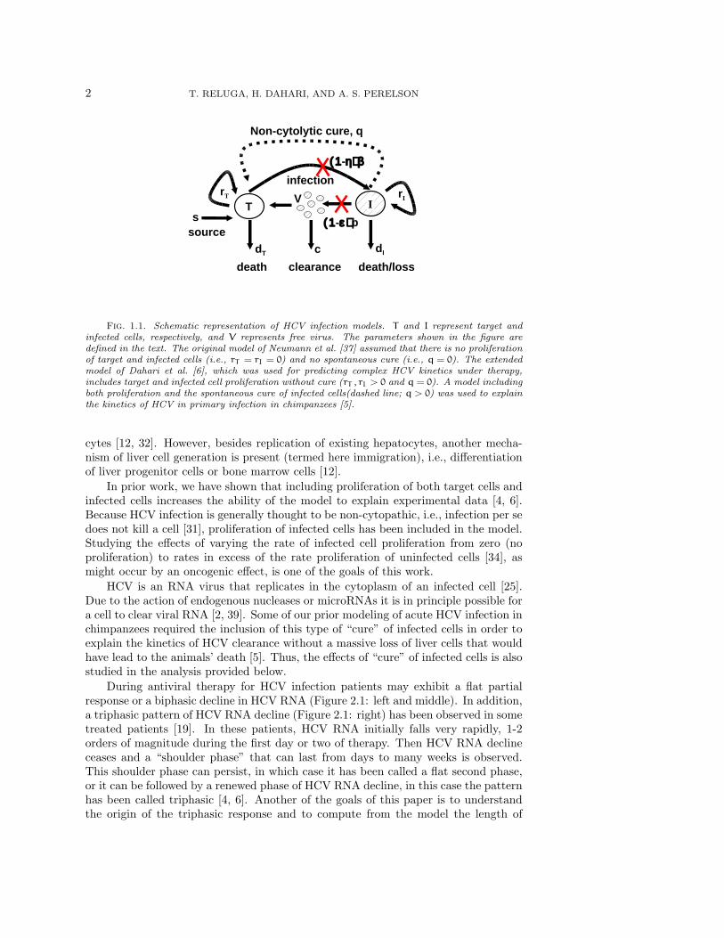
A model of human immunodeficiency virus infection [40, 52] was adapted byNeumann et al. [37] to study the kinetics of chronic HCV infection during treatment.Since then viral kinetics modeling has played an important role in the analysis ofHCV RNA decay during antiviral therapy (see Perelson [41], Perelson et al. [42] ).The original Neumann et al. model for HCV infection [37] included three differentialequations representing the populations of target cells, productively-infected cells, andvirus (Figure 1.1). A simplified version of the model, which assumes a constantpopulation of target cells, was used to estimate the rates of viral clearance and infectedcell loss by fitting to the model the decline of HCV RNA observed in patients duringthe first 14 days of therapy [37]. However, this simplified version of the model is notable to explain some observed HCV RNA kinetic profiles under treatment [4]. Tomodel complex HCV kinetics, the assumption of a constant level of target cells needsto be relaxed and requires one to model as correctly as possible the dynamics of thetarget cell population. Since it has been suggested that hepatocytes, the major celltype in the liver, are also the major producers of HCV [10, 3, 43], we assume herethat the target cells of the model are hepatocytes.

The liver is an organ that regenerates, and due to homeostatic mechanisms, anyloss of hepatocytes would be compensated for by the proliferation of existing hepato-

‡ Portions of this work were done under the auspices of the U. S. Department of Energy undercontract DE-AC52-06NA25396 and supported by NIH grants AI28433, RR06555, AI06525, and P20-RR18754 and the Human Frontiers Science Program grant RPG0010/2004.

§Current address: Department of Mathematics, Pennsylvania State University, University ParkPA 16802,¶Current address: Department of Medicine, University of Illinois at Chicago, Chicago, IL 60612,

1

2 T. RELUGA, H. DAHARI, AND A. S. PERELSON

I T

death/lossclearance

c

V

dT

death

source

infection

( 1-ε ) p

rT rI

Non-cytolytic cure, q

s

( 1-η) β

dI

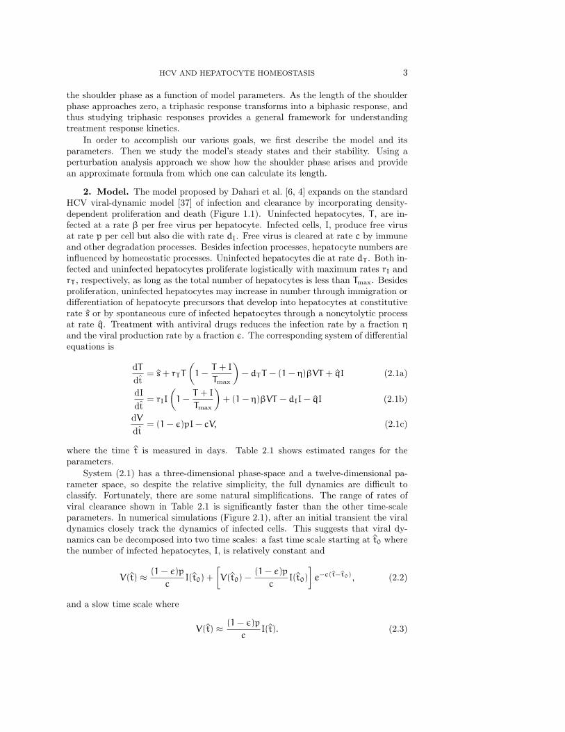
Fig. 1.1. Schematic representation of HCV infection models. T and I represent target andinfected cells, respectively, and V represents free virus. The parameters shown in the figure aredefined in the text. The original model of Neumann et al. [37] assumed that there is no proliferationof target and infected cells (i.e., rT = rI = 0) and no spontaneous cure (i.e., q = 0). The extendedmodel of Dahari et al. [6], which was used for predicting complex HCV kinetics under therapy,includes target and infected cell proliferation without cure (rT , rI > 0 and q = 0). A model includingboth proliferation and the spontaneous cure of infected cells(dashed line; q > 0) was used to explainthe kinetics of HCV in primary infection in chimpanzees [5].

cytes [12, 32]. However, besides replication of existing hepatocytes, another mecha-nism of liver cell generation is present (termed here immigration), i.e., differentiationof liver progenitor cells or bone marrow cells [12].

In prior work, we have shown that including proliferation of both target cells andinfected cells increases the ability of the model to explain experimental data [4, 6].Because HCV infection is generally thought to be non-cytopathic, i.e., infection per sedoes not kill a cell [31], proliferation of infected cells has been included in the model.Studying the effects of varying the rate of infected cell proliferation from zero (noproliferation) to rates in excess of the rate proliferation of uninfected cells [34], asmight occur by an oncogenic effect, is one of the goals of this work.

HCV is an RNA virus that replicates in the cytoplasm of an infected cell [25].Due to the action of endogenous nucleases or microRNAs it is in principle possible fora cell to clear viral RNA [2, 39]. Some of our prior modeling of acute HCV infection inchimpanzees required the inclusion of this type of “cure” of infected cells in order toexplain the kinetics of HCV clearance without a massive loss of liver cells that wouldhave lead to the animals’ death [5]. Thus, the effects of “cure” of infected cells is alsostudied in the analysis provided below.

During antiviral therapy for HCV infection patients may exhibit a flat partialresponse or a biphasic decline in HCV RNA (Figure 2.1: left and middle). In addition,a triphasic pattern of HCV RNA decline (Figure 2.1: right) has been observed in sometreated patients [19]. In these patients, HCV RNA initially falls very rapidly, 1-2orders of magnitude during the first day or two of therapy. Then HCV RNA declineceases and a “shoulder phase” that can last from days to many weeks is observed.This shoulder phase can persist, in which case it has been called a flat second phase,or it can be followed by a renewed phase of HCV RNA decline, in this case the patternhas been called triphasic [4, 6]. Another of the goals of this paper is to understandthe origin of the triphasic response and to compute from the model the length of

HCV AND HEPATOCYTE HOMEOSTASIS 3

the shoulder phase as a function of model parameters. As the length of the shoulderphase approaches zero, a triphasic response transforms into a biphasic response, andthus studying triphasic responses provides a general framework for understandingtreatment response kinetics.

In order to accomplish our various goals, we first describe the model and itsparameters. Then we study the model’s steady states and their stability. Using aperturbation analysis approach we show how the shoulder phase arises and providean approximate formula from which one can calculate its length.

2. Model. The model proposed by Dahari et al. [6, 4] expands on the standardHCV viral-dynamic model [37] of infection and clearance by incorporating density-dependent proliferation and death (Figure 1.1). Uninfected hepatocytes, T , are in-fected at a rate β per free virus per hepatocyte. Infected cells, I, produce free virusat rate p per cell but also die with rate dI. Free virus is cleared at rate c by immuneand other degradation processes. Besides infection processes, hepatocyte numbers areinfluenced by homeostatic processes. Uninfected hepatocytes die at rate dT . Both in-fected and uninfected hepatocytes proliferate logistically with maximum rates rI andrT , respectively, as long as the total number of hepatocytes is less than Tmax. Besidesproliferation, uninfected hepatocytes may increase in number through immigration ordifferentiation of hepatocyte precursors that develop into hepatocytes at constitutiverate s or by spontaneous cure of infected hepatocytes through a noncytolytic processat rate q. Treatment with antiviral drugs reduces the infection rate by a fraction ηand the viral production rate by a fraction ε. The corresponding system of differentialequations is

dTdt

= s+ rTT

(1−

T + I

Tmax

)− dTT − (1− η)βVT + qI (2.1a)

dIdt

= rII

(1−

T + I

Tmax

)+ (1− η)βVT − dII− qI (2.1b)

dVdt

= (1− ε)pI− cV, (2.1c)

where the time t is measured in days. Table 2.1 shows estimated ranges for theparameters.

System (2.1) has a three-dimensional phase-space and a twelve-dimensional pa-rameter space, so despite the relative simplicity, the full dynamics are difficult toclassify. Fortunately, there are some natural simplifications. The range of rates ofviral clearance shown in Table 2.1 is significantly faster than the other time-scaleparameters. In numerical simulations (Figure 2.1), after an initial transient the viraldynamics closely track the dynamics of infected cells. This suggests that viral dy-namics can be decomposed into two time scales: a fast time scale starting at t0 wherethe number of infected hepatocytes, I, is relatively constant and

V(t) ≈ (1− ε)p

cI(t0) +

[V(t0) −

(1− ε)p

cI(t0)

]e−c(t−t0), (2.2)

and a slow time scale where

V(t) ≈ (1− ε)p

cI(t). (2.3)


Table 2.1Estimated parameter ranges for hepatitis C when modelled with System (2.1). The columns

labelled left, middle, and right give the parameter values for fitting System (2.1) to the data for therespective plots in Figure 2.1. The rT ,Tmax, and dT parameters are not independently identifiable,so common practice is to fix dT prior to fitting.

Symbol Minimum Maximum Units left middle right Referenceβ 10−8 10−6 virus−1 ml day−1 1.4× 10−6 9.0× 10−8 2.8× 10−8 [5]Tmax 4× 106 1.3× 107 cells ml−1 5× 106 5× 106 1.2× 107 [27, 49]p 0.1 44 virus cell−1 day−1 28.7 10.9 13.2 [5]s 1 1.8× 105 cells ml−1 day−1 1 1 1 [50]q 0 1 day−1 0 0 0 [5]c 0.8 22 day−1 6.0 5.8 5.4 [45]dT 10−3 1.4× 10−2 day−1 1.2× 10−2 1.2× 10−2 1.2× 10−2 [26, 28]dI 10−3 0.5 day−1 0.36 0.48 0.13 [45]rT 2× 10−3 3.4 day−1 3.0 0.70 1.1 [5]rI Unknown Unknown day−1 .97 0.112 0.26

103

104

105

106

107

0 2 4 6 8 10 12 14Viru

s C

once

ntra

tion

( m

l-1)

Time (days after treatment starts)

Flat partial response

103

104

105

106

107

0 2 4 6 8 10 12 14


Biphasic response

103

104

105

106

107

0 5 10 15 20 25 30


Triphasic response

Infected HepatocytesUninfected Hepatocytes

Fig. 2.1. Three example plots of observed changes in viral load (X) following the start oftreatment, together with numerical solutions to System (2.1) (solid line). The initial condition ofeach numerical solutions is the chronic-infection steady-state. In some cases, there is a flat partialresponse to treatment (left), where viral load shows an immediate drop, but then remains unchangedover time. In some cases, there is a biphasic response (middle), with a rapid initial drop and aslower asymptotic clearance. In some cases, there is a triphasic response, with a rapid initial drop,an intermediate shoulder phase during which there is little change, and then an asymptotic clearancephase. The initial rapid decline in virus load is the synchronization to the new quasi-steady state,following the start of treatment. Afterward, virus load closely tracks the number of infected cells(right). Treatment efficacies are ε = 0.98, η = 0 (left), ε = 0.9, η = 0 (middle), and ε = 0.996, η = 0(right). Other parameter values are shown in Table 2.1.

For patients in steady state before treatment, as is typically the case, I(t0) = cV(t0)/p,allowing one to simply Equation (2.2) to

V(t) = (1− ε)V(t0) + εV(t0)e−c(t−t0). (2.4)

On times scales longer than 1/c, then, the dynamics of System (2.1) can beapproximated by a system of two equations. If we now introduce the dimensionlesstime t = (rT − dT )t, the dimensionless state variables

x =T

Tmax, y =

I

Tmax, (2.5)


and the dimensionless parameters

s =srT

(rT − dT )2Tmax, b =

pβTmax

crT, q =

q

rT − dT,

r =rI

rT, d =

dIrT − dT rI

rT (rT − dT ), 1− θ = (1− ε)(1− η),

(2.6)

then under the quasi-steady state approximation, System (2.1) is equivalent to thedimensionless system

x = x (1− x− y) − (1− θ)byx+ qy+ s, (2.7a)y = ry (1− x− y) + (1− θ)byx− dy− qy. (2.7b)

Note that a fundamental assumption in the transformation to System (2.7) is thatrT > dT , which we expect because of the hepatocyte population’s ability to supportitself and to regenerate itself after injury.

Immigration of new hepatocytes is believed to be slow (< 1% per day; Table 1)relative to the total number of hepatocytes (i.e., s � 1). Spontaneous cure fromHCV has not yet been directly observed. It has been suggested to occur based on thekinetics of HCV clearance and liver damage in humans [51] and in chimpanzees [5].Therefore, in a first analysis, we assume that s = q = 0. Later, we reintroduce theseparameters and examine their effects via a perturbation analysis. Dropping the s andq terms, System (2.7) simplifies to

x = x (1− x− y) − (1− θ)byx, (2.8a)y = ry (1− x− y) + (1− θ)byx− dy. (2.8b)

Most of the parameter ranges from Table 2.1 are captured by allowing b ∈ [10−2, 103]and d ∈ [10−3, 102]. rI has not yet been studied experimentally, and thus we can notbound r beyond the trivial statement that r ≥ 0.

Gomez-Acevedo and Li [14] have previously studied some of the properties ofSystem (2.8) in the context of human T-cell lymphotropic virus type I. It is a simplemodel with only three independent parameters and dynamics that can be completelyanalyzed using phase-plane analysis and algebraic methods while still encapsulatingthe fundamental concepts of System (2.1). System (2.8) diverges from common viraldynamics models in the homeostasis parameter r. When r = 0, System (2.8) isnaturally interpreted as an epidemic model, a viral infection model, or a predator-prey model. When the epidemic model is extended to include logistic homeostasis withr > 0, the infected cells can also proliferate independent of x but experience additionaldensity-dependent mortality as a function of the total population size x+y. This paperexplores the consequences of this homeostasis. We will first study System (2.7) andSystem (2.8) during acute infection. We will then study the response of these systemsto treatment.

3. Dynamics without treatment (θ = 0). When hepatitis C virus first infectsa person, the ensuing dynamics depend on the relative parameter values. Since newlyinfected individuals do not know that they are infected, we assume there is initiallyno treatment (θ = 0). At first glance, we might expect several different scenariosto ensue, following exposure: infection may fade out without becoming established,infection may spread with limited success and infect only part of the liver, or infectionmay spread rapidly and infect the whole liver. To understand when the dynamics ofSystem (2.7) under acute infection correspond to each of these situations, it is helpfulto walk through the bifurcation structure of System (2.8).


1-d/r

1/(1+b)

1

(d-r)/(b-r) 1

x

No Infection

b=0.1d=0.4r=0.8

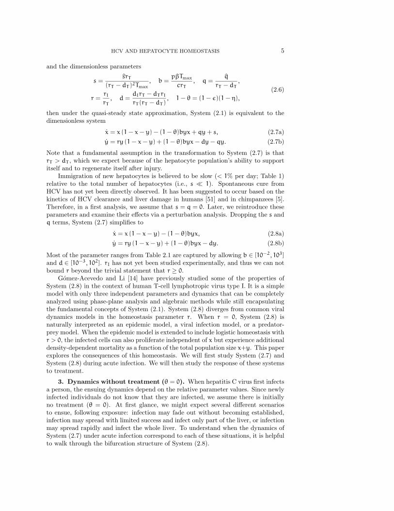
Fig. 3.1. Example nullclines for System (2.8) when the disease-free equilibrium is globallyattracting. The liver-free (x = y = 0), disease-free (x = 1, y = 0), and total-infection (x = 0, y =1 − d/r) stationary solutions are marked with dots. The solid lines are the y-nullclines, the dottedlines are the x-nullclines. The partial-infection stationary solution is not present for these parametervalues.

0

0.2

0.4

0.6

0.8

1

1.2

0 0.2 0.4 0.6 0.8 1 1.2

Cle

aran

ce r

ate

(d)

Transmission rate (b)

No Infection

Total Infection

PartialInfection

Oscillations

r=0.8

0

0.5

1

1.5

2

2.5

3

0 0.5 1 1.5 2 2.5


No Infection

Total Infection

Bistable

Partial

r=2.5

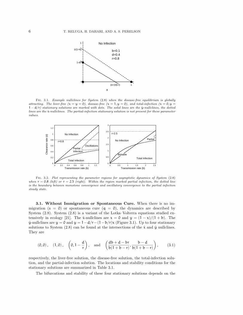
Fig. 3.2. Plot representing the parameter regions for asymptotic dynamics of System (2.8)when r = 0.8 (left) or r = 2.5 (right). Within the region marked partial infection, the dotted lineis the boundary between monotone convergence and oscillatory convergence to the partial infectionsteady state.

3.1. Without Immigration or Spontaneous Cure. When there is no im-migration (s = 0) or spontaneous cure (q = 0), the dynamics are described bySystem (2.8). System (2.8) is a variant of the Lotka–Volterra equations studied ex-tensively in ecology [21]. The x-nullclines are x = 0 and y = (1 − x)/(1 + b). They-nullclines are y = 0 and y = 1−d/r−(1−b/r)x (Figure 3.1). Up to four stationarysolutions to System (2.8) can be found at the intersections of the x and y nullclines.They are

(0, 0) , (1, 0) ,

(0, 1−

d

r

), and

(db+ d− br

b(1+ b− r),

b− d

b(1+ b− r)

), (3.1)

respectively, the liver-free solution, the disease-free solution, the total-infection solu-tion, and the partial-infection solution. The locations and stability conditions for thestationary solutions are summarized in Table 3.1.

The bifurcations and stability of these four stationary solutions depends on the


0

0.2

0.4

0.6

0.8

1

0 0.2 0.4 0.6 0.8 1

y

x

Total Infectionb=0.45d=0.20r=0.8

0

0.2

0.4

0.6

0.8

1

0 0.2 0.4 0.6 0.8 1

y

x

Partial Infectionb=0.45d=0.40r=0.8

0

0.2

0.4

0.6

0.8

1

0 0.2 0.4 0.6 0.8 1

y

x

Bistableb=1d=1.2r=3

0

0.2

0.4

0.6

0.8

1

0 0.2 0.4 0.6 0.8 1

y

x

Partial Infection with Oscillationsb=1.20d=0.90r=0.8

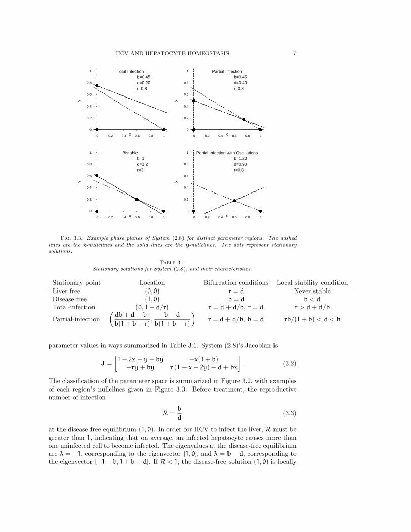
Fig. 3.3. Example phase planes of System (2.8) for distinct parameter regions. The dashedlines are the x-nullclines and the solid lines are the y-nullclines. The dots represent stationarysolutions.

Table 3.1Stationary solutions for System (2.8), and their characteristics.

Stationary point Location Bifurcation conditions Local stability conditionLiver-free (0, 0) r = d Never stableDisease-free (1, 0) b = d b < d

Total-infection (0, 1− d/r) r = d+ d/b, r = d r > d+ d/b

Partial-infection(db+ d− br

b(1+ b− r),

b− d

b(1+ b− r)

)r = d+ d/b, b = d rb/(1+ b) < d < b

parameter values in ways summarized in Table 3.1. System (2.8)’s Jacobian is

J =

[1− 2x− y− by −x(1+ b)

−ry+ by r (1− x− 2y) − d+ bx

]. (3.2)

The classification of the parameter space is summarized in Figure 3.2, with examplesof each region’s nullclines given in Figure 3.3. Before treatment, the reproductivenumber of infection

R =b

d(3.3)

at the disease-free equilibrium (1, 0). In order for HCV to infect the liver, R must begreater than 1, indicating that on average, an infected hepatocyte causes more thanone uninfected cell to become infected. The eigenvalues at the disease-free equilibriumare λ = −1, corresponding to the eigenvector [1, 0], and λ = b − d, corresponding tothe eigenvector [−1− b, 1+ b− d]. If R < 1, the disease-free solution (1, 0) is locally


attracting. If R > 1, HCV infects new cells faster than infected cells die, and theasymptotic dynamics may correspond to either partial or total infection of the liver.

The liver-free stationary solution (0, 0) is always unstable, switching between asaddle point when infected cells die quickly (r < d) and an unstable node wheninfected cells die slowly (d < r). If the proliferation rate is slower than the deathrate (r < d), then HCV can never totally infect the liver. There is a transcriticalbifurcation at d = r, and the total-infection stationary solution (0, 1− d/r) is only afeasible when the proliferation rate of infected cells is greater than the excess deathrate of infected cells (Figure 3.2). From the Jacobian, we see that if d + d/b < r

(equivalently, d < rb/(1 + b)), total infection is locally stable, and from the general

theory of Lotka–Volterra systems, it is globally stable provided d < min{b,rb

1+ b}.

This includes all cases where d < 0.The partial-infection stationary solution is present whenever d lies between b

andrb

1+ b. The local stability of the partially-infected stationary solution can be

determined from the characteristic polynomial

λ2 +d

bλ+

(d− b)(br− bd− d)

b(1+ b− r)= 0, (3.4)

where λ is an eigenvalue. If b < d <rb

1+ b, the constant term of the characteris-

tic polynomial at the partial-infection stationary solution is negative, implying (byDecartes’ rule of sign) that there is a single positive root and the partial-infectionsteady-state is a saddle point. In this situation, we can show that both the disease-free and the total-infection stationary solutions are locally stable. As first shownin Gomez-Acevedo and Li [14], the system is bistable and the asymptotic dynamicswill depend in the initial conditions. The constraint r < 1 is sufficient to precludebistability.

When b > d >rb

1+ b, the coefficients d/b and

(d− b)(br− bd− d)

b(1+ b− r)(3.5)

of the characteristic polynomial are both positive. From the Routh–Hurwitz con-ditions [35], it follows immediately that the partial-infection stationary solution islocally stable. From prior work on Lotka–Volterra equations [20], we know that it isalso globally stable.

Convergence to the partial-infection stationary solution can be oscillatory if theeigenvalues are complex or monotone if the eigenvalues are real (Figure 3.4). Calcu-lation of the discriminant shows that the convergence is oscillatory whenever

d2

4b2−

(b− d)(rb− db− d)

b(r− 1− b)< 0. (3.6)

This inequality is not easy to interpret by inspection, but it is quadratic in d, so it iseasy to handle numerically. The boundaries of the subset of parameter space whereconvergence is oscillatory asymptotically converge to d(b) = r and d(b) = b as bdiverges to ∞. When convergence is oscillatory, the period of oscillations around the


0.01

0.1

1

0 10 20 30 40 50 60

Stat

e

Time (t)

xy

0.01

0.1

1

0 10 20 30 40 50 60Time (t)

xy

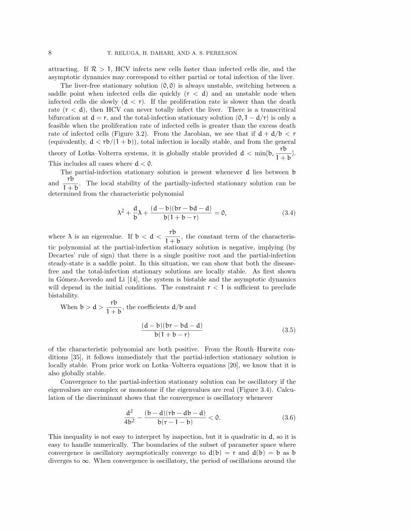
Fig. 3.4. Time series for System (2.7) of monotone (left, r = 0.6, b = 0.6) and oscillatory(right, r = 0.1, b = 2.6) convergence to the partial infection stationary solution when d = 0.4.

0

1-d/r

1/(1+b)

1

0 (r-d)/(r-b) 1

x

y

b=0.1d=0.4r=0.8s=0.001q=0.001

0 (r-d)/(r-b) 1

x

b=0.1d=0.4r=0.8s=0.02q=0.02

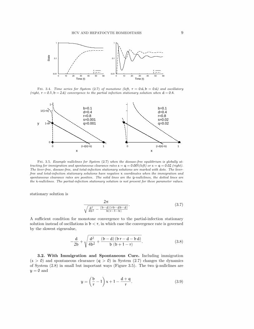
Fig. 3.5. Example nullclines for System (2.7) when the disease-free equilibrium is globally at-tracting for immigration and spontaneous clearance rates s = q = 0.001(left) or s = q = 0.02 (right).The liver-free, disease-free, and total-infection stationary solutions are marked with dots. The liver-free and total-infection stationary solutions have negative x coordinates when the immigration andspontaneous clearance rates are positive. The solid lines are the y-nullclines, the dotted lines arethe x-nullclines. The partial-infection stationary solution is not present for these parameter values.

stationary solution is

2π√d2

4b2 −(b−d)(rb−db−d)

b(r−1−b)

. (3.7)

A sufficient condition for monotone convergence to the partial-infection stationarysolution instead of oscillations is b < r, in which case the convergence rate is governedby the slowest eigenvalue,

−d

2b+

√d2

4b2+

(b− d) (b r− d− bd)

b (b+ 1− r). (3.8)

3.2. With Immigration and Spontaneous Cure. Including immigration(s > 0) and spontaneous clearance (q > 0) in System (2.7) changes the dynamicsof System (2.8) in small but important ways (Figure 3.5). The two y-nullclines arey = 0 and

y =

(b

r− 1

)x+ 1−

d+ q

r. (3.9)


Spontaneous clearance moves the nullcline given by Eq. (3.9) slightly to the left, butthe y-nullclines are basically the same as those of System (2.8). The change in thex-nullclines is more pronounced. The only x-nullcline in System (2.7) is

y =s+ x(1− x)

x+ bx− q. (3.10)

The x-nullclines have changed from a pair of intersecting lines in System (2.8) to ahyperbola in System (2.7). The shape of the hyperbola is still the same as those ofSystem (2.8) except near the intersection point (0, 1 − d/r). The hyperbola is alsoshifted slightly down and to the right compared to System (2.8) (Figure 3.5). For largepositive and negative x, the nullcline is approximately equal to (1−x)/(1+b). Thereis a vertical asymptote at x = q/(1+ b). The nullcline is positive just to the right ofthis asymptote and negative just to it’s left. The x-nullcline’s unique y-intercept isy = −s/q. This implies that there can be no biologically feasible stationary solutionswith x ≤ q/(1 + b), i.e. , total hepatocyte loss is no longer a stationary solutionbecause the model now includes a perpetual source of new hepatocytes. This changealso means that there is no longer a bifurcation between partial and total infection(Figure 3.6).

Two stationary solutions to System (2.7) solve

x2 − x− s = 0 with y = 0. (3.11)

The exact solutions are (1±√1+ 4s

2, 0

). (3.12)

When s is very small, the solutions of Eq. (3.11) are approximately

(−s+ o(s), 0) and (1+ s+ o(s), 0). (3.13)

The solution with the negative square root can never appear biologically because itpredicts a negative number of uninfected hepatocytes.

The other two stationary solutions of System (2.7) solve

b (1+ b− r) x2 + [(rb− db− d) + q (r− 1− 2 b)] x− sr− (r− d− q)q = 0,

(3.14a)

with y =

(b

r− 1

)x+ 1−

d+ q

r. (3.14b)

The solutions can be expressed in terms of radicals, but greater intuition of the effectsof s and q relative to the stationary solutions of System (2.8) can be gained thoughperturbation analysis (Appendix A). When d < min{b, rb/(1+b)}, the one biologicallymeaningful solution to Eq. (3.14) is

(x, y) =

(q(r− d) + sr

rb− bd− d+ o(s, q), 1−

d

r+

(r− b) s

d+ bd− br−

(r2 − rd− d

)q

r (−d− bd+ br)+ o(s, q)

),

(3.15)

corresponding to the total-infection stationary solution of System (2.8), but with asmall number of uninfected cells sustained by the sources s and q. The o(s, q) terms


in Eq. (3.16) hide higher order effects in s and q that vanish quadratically or fasteras s and q approach zero. When rb/(1+ b) < d < b,

x =d+ db− rb

b (1+ b− r)−

rs

rb− d− db+

(rb2 + rd− d− 2db− db2

)b (1+ b− r) (rb− d− db)

q+ o(s, q) (3.16a)

y =b− d

b (1+ b− r)−

s (b− r)

rb− d− db−

(b2 − 2 db+ rd− d

)q

b (1+ b− r) (rb− d− db)+ o(s, q) (3.16b)

is an approximate solution corresponding to the partial-infection stationary solutionof System (2.8). The other solution of 3.14 is negative.

When b < d < rb/(1 + b), both solutions to Eq. (3.14) are positive. Again, thiscan only occur when r > 1, i.e., when infected cells proliferate faster than uninfectedones. Approximate locations are given by Eq. (3.15) and Eq. (3.16). The bifurcationbetween zero and two roots is a saddle-node bifurcation where the root with smallerx value is a stable node and the root with larger x value is a saddle. The calculationof the exact condition for bistability when s or q is positive is algebraically opaque,requiring the solution of a pair of polynomials that are quadratic in d and a test todistinguish bistability outside the positive quadrant from bistability inside the positivequadrant. The net effect in System (2.7) of this complexity is a minor perturbationof that found for System (2.8) (compare Figures 3.2 and Figure 3.6). Immigrationand spontaneous clearance shrink the bistable region of parameter space slightly andshift it so that it occurs for slightly smaller values of d.

The local stability of the stationary solutions to System (2.7) is predicted by theJacobian matrix

J =

[1− 2x− y− by −x(1+ b) + q

−ry+ by r (1− x− 2y) − d+ bx− q

]. (3.17)

The disease-free stationary solution loses stability through a transcritical bifurcationthat occurs at det J = 0. Substituting y = 0 into J, det J = 0 if x = 1/2 or(b− r)x = d+q− r. Using the approximation x = 1+ s+ o(s), we can show that thedisease-free stationary solution is stable when

(1+ s)b < d+ q+ rs+ o(s). (3.18)

Local stability of the other stationary solutions to System (2.7) can also be approxi-mated analytically, but resulting formulas are difficult to interpret.

4. Treatment Effects. Treatment effects appear in System (2.7) and System (2.8)only through a multiplicative factor (1 − θ) reducing the transmission rate b, whereθ is the dimensionless treatment efficacy. Thus, the stationary solution structure ofSystem (2.7) and System (2.8) under treatment is summarized by replacing the x-axislabels in Figures 3.2 and 3.6 by (1 − θ)b. Taking b to be constant, the outcome ofdrug treatment depends on the drug efficacy θ (Table 4.1, Figure 4.1). There is acritical efficacy

θc ≈

{1− d+q+rs

(1+s)b if r < d+ 1,

1− d(r−d)b if r > d+ 1.

(4.1)

such that θ > θc implies treatment will clear the infection. When r < d+1, the criticalefficacy θc corresponds to reducing the reproductive number to 1. When r > d+1, the


0

0.2

0.4

0.6

0.8

1

1.2

0 0.2 0.4 0.6 0.8 1 1.2

Cle

aran

ce r

ate

(d)


No Infection

Infection

DampedOscillations

r=0.8

0

0.5

1

1.5

2

2.5

0 0.5 1 1.5 2 2.5


No Infection

BistableInfection

r=2.5

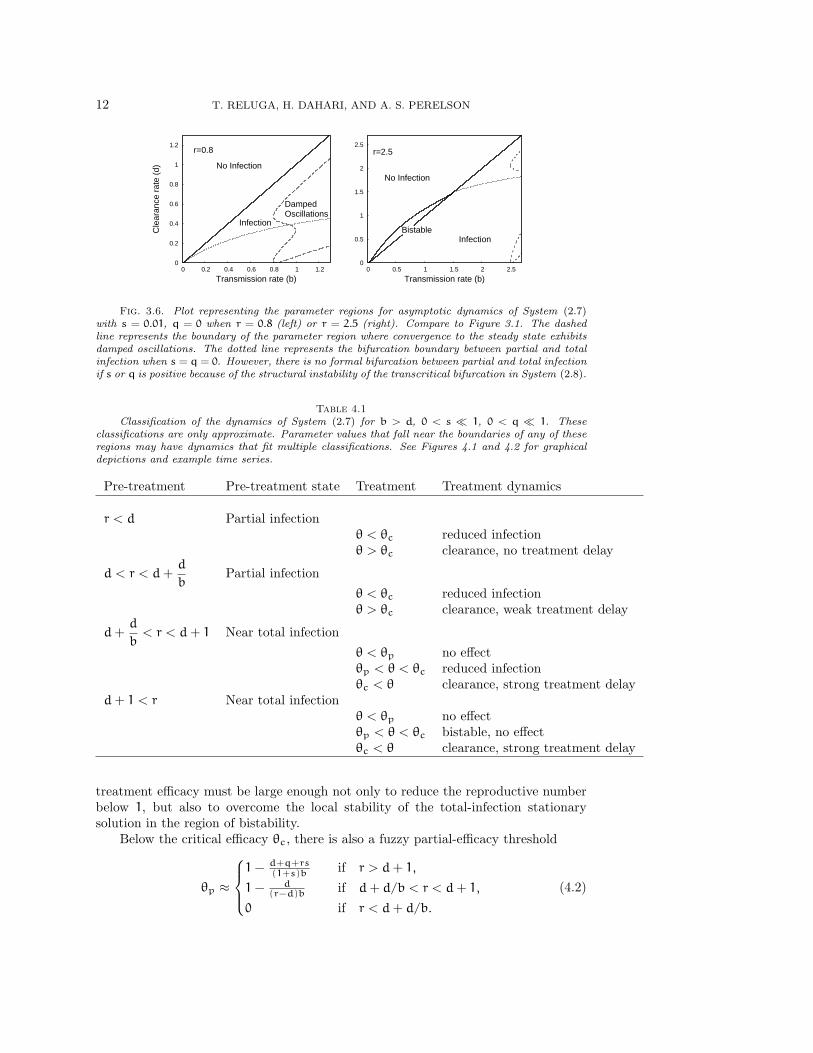
Fig. 3.6. Plot representing the parameter regions for asymptotic dynamics of System (2.7)with s = 0.01, q = 0 when r = 0.8 (left) or r = 2.5 (right). Compare to Figure 3.1. The dashedline represents the boundary of the parameter region where convergence to the steady state exhibitsdamped oscillations. The dotted line represents the bifurcation boundary between partial and totalinfection when s = q = 0. However, there is no formal bifurcation between partial and total infectionif s or q is positive because of the structural instability of the transcritical bifurcation in System (2.8).

Table 4.1Classification of the dynamics of System (2.7) for b > d, 0 < s � 1, 0 < q � 1. These

classifications are only approximate. Parameter values that fall near the boundaries of any of theseregions may have dynamics that fit multiple classifications. See Figures 4.1 and 4.2 for graphicaldepictions and example time series.

Pre-treatment Pre-treatment state Treatment Treatment dynamics

r < d Partial infectionθ < θc reduced infectionθ > θc clearance, no treatment delay

d < r < d+d

bPartial infection

θ < θc reduced infectionθ > θc clearance, weak treatment delay

d+d

b< r < d+ 1 Near total infection

θ < θp no effectθp < θ < θc reduced infectionθc < θ clearance, strong treatment delay

d+ 1 < r Near total infectionθ < θp no effectθp < θ < θc bistable, no effectθc < θ clearance, strong treatment delay

treatment efficacy must be large enough not only to reduce the reproductive numberbelow 1, but also to overcome the local stability of the total-infection stationarysolution in the region of bistability.

Below the critical efficacy θc, there is also a fuzzy partial-efficacy threshold

θp ≈

1− d+q+rs

(1+s)b if r > d+ 1,

1− d(r−d)b if d+ d/b < r < d+ 1,

0 if r < d+ d/b.

(4.2)


0

0.2

0.4

0.6

0.8

1

0.3 d=.5 d/(r-d)=1.25 8

Tre

atm

ent e

ffica

cy (

θ)


Clearance

ReducedInfection

No Effect

θcθp

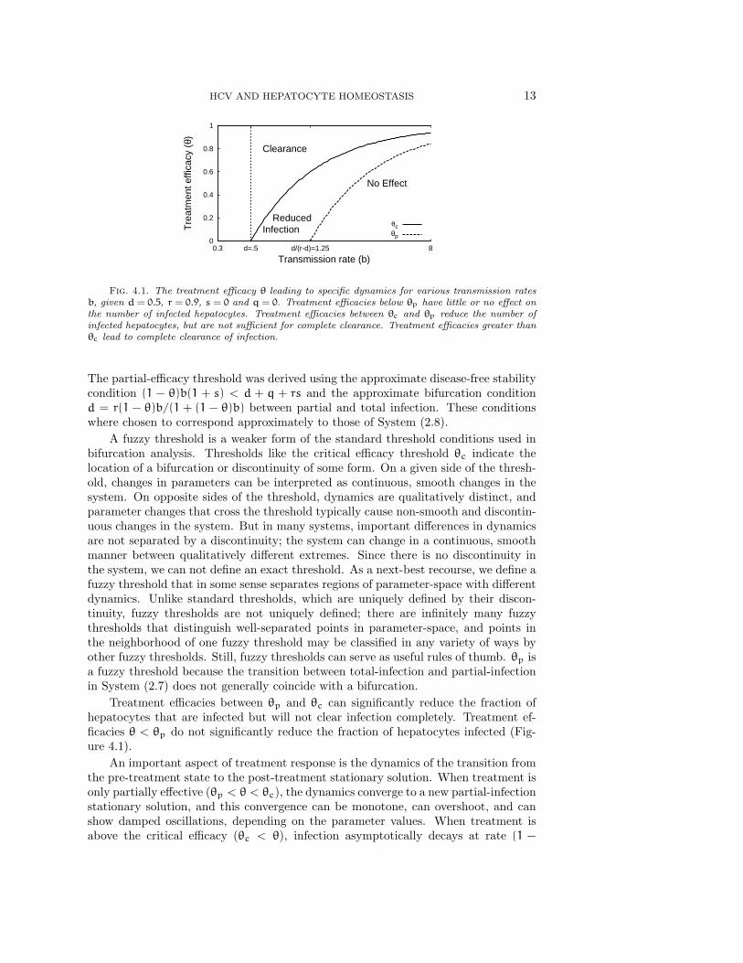
Fig. 4.1. The treatment efficacy θ leading to specific dynamics for various transmission ratesb, given d = 0.5, r = 0.9, s = 0 and q = 0. Treatment efficacies below θp have little or no effect onthe number of infected hepatocytes. Treatment efficacies between θc and θp reduce the number ofinfected hepatocytes, but are not sufficient for complete clearance. Treatment efficacies greater thanθc lead to complete clearance of infection.

The partial-efficacy threshold was derived using the approximate disease-free stabilitycondition (1 − θ)b(1 + s) < d + q + rs and the approximate bifurcation conditiond = r(1 − θ)b/(1 + (1 − θ)b) between partial and total infection. These conditionswhere chosen to correspond approximately to those of System (2.8).

A fuzzy threshold is a weaker form of the standard threshold conditions used inbifurcation analysis. Thresholds like the critical efficacy threshold θc indicate thelocation of a bifurcation or discontinuity of some form. On a given side of the thresh-old, changes in parameters can be interpreted as continuous, smooth changes in thesystem. On opposite sides of the threshold, dynamics are qualitatively distinct, andparameter changes that cross the threshold typically cause non-smooth and discontin-uous changes in the system. But in many systems, important differences in dynamicsare not separated by a discontinuity; the system can change in a continuous, smoothmanner between qualitatively different extremes. Since there is no discontinuity inthe system, we can not define an exact threshold. As a next-best recourse, we define afuzzy threshold that in some sense separates regions of parameter-space with differentdynamics. Unlike standard thresholds, which are uniquely defined by their discon-tinuity, fuzzy thresholds are not uniquely defined; there are infinitely many fuzzythresholds that distinguish well-separated points in parameter-space, and points inthe neighborhood of one fuzzy threshold may be classified in any variety of ways byother fuzzy thresholds. Still, fuzzy thresholds can serve as useful rules of thumb. θp isa fuzzy threshold because the transition between total-infection and partial-infectionin System (2.7) does not generally coincide with a bifurcation.

Treatment efficacies between θp and θc can significantly reduce the fraction ofhepatocytes that are infected but will not clear infection completely. Treatment ef-ficacies θ < θp do not significantly reduce the fraction of hepatocytes infected (Fig-ure 4.1).

An important aspect of treatment response is the dynamics of the transition fromthe pre-treatment state to the post-treatment stationary solution. When treatment isonly partially effective (θp < θ < θc), the dynamics converge to a new partial-infectionstationary solution, and this convergence can be monotone, can overshoot, and canshow damped oscillations, depending on the parameter values. When treatment isabove the critical efficacy (θc < θ), infection asymptotically decays at rate (1 −


10-4

10-3

10-2

10-1

100

-5 0 5 10 15 20 25

Sta

te

Time from treatment’s start (1/(rT-dT) units)

No Delay

r=0

xy

10-4

10-3

10-2

10-1

100

-5 0 5 10 15 20 25

Sta

te

Weak Delay

r=0.3

xy

10-4

10-3

10-2

10-1

100

-5 0 5 10 15 20 25

Sta

te

Strong Delay

r=0.6

xy

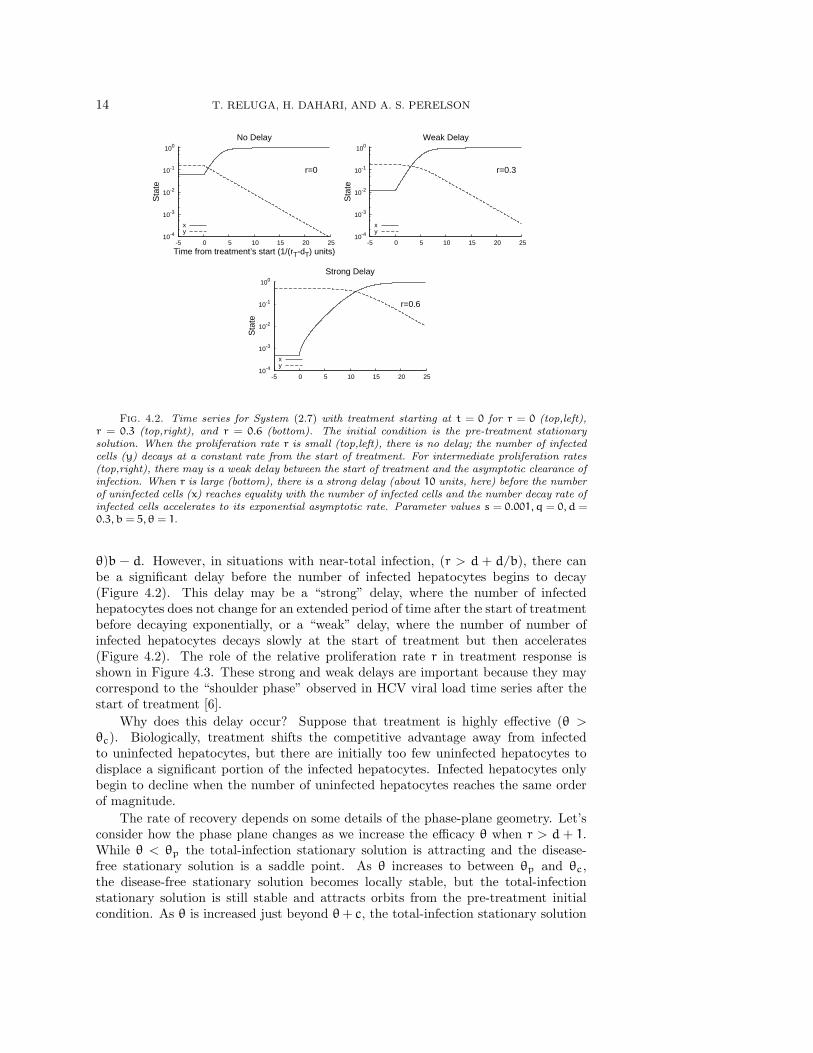
Fig. 4.2. Time series for System (2.7) with treatment starting at t = 0 for r = 0 (top,left),r = 0.3 (top,right), and r = 0.6 (bottom). The initial condition is the pre-treatment stationarysolution. When the proliferation rate r is small (top,left), there is no delay; the number of infectedcells (y) decays at a constant rate from the start of treatment. For intermediate proliferation rates(top,right), there may is a weak delay between the start of treatment and the asymptotic clearance ofinfection. When r is large (bottom), there is a strong delay (about 10 units, here) before the numberof uninfected cells (x) reaches equality with the number of infected cells and the number decay rate ofinfected cells accelerates to its exponential asymptotic rate. Parameter values s = 0.001, q = 0, d =0.3, b = 5, θ = 1.

θ)b − d. However, in situations with near-total infection, (r > d + d/b), there canbe a significant delay before the number of infected hepatocytes begins to decay(Figure 4.2). This delay may be a “strong” delay, where the number of infectedhepatocytes does not change for an extended period of time after the start of treatmentbefore decaying exponentially, or a “weak” delay, where the number of number ofinfected hepatocytes decays slowly at the start of treatment but then accelerates(Figure 4.2). The role of the relative proliferation rate r in treatment response isshown in Figure 4.3. These strong and weak delays are important because they maycorrespond to the “shoulder phase” observed in HCV viral load time series after thestart of treatment [6].

Why does this delay occur? Suppose that treatment is highly effective (θ >θc). Biologically, treatment shifts the competitive advantage away from infectedto uninfected hepatocytes, but there are initially too few uninfected hepatocytes todisplace a significant portion of the infected hepatocytes. Infected hepatocytes onlybegin to decline when the number of uninfected hepatocytes reaches the same orderof magnitude.

The rate of recovery depends on some details of the phase-plane geometry. Let’sconsider how the phase plane changes as we increase the efficacy θ when r > d + 1.While θ < θp the total-infection stationary solution is attracting and the disease-free stationary solution is a saddle point. As θ increases to between θp and θc,the disease-free stationary solution becomes locally stable, but the total-infectionstationary solution is still stable and attracts orbits from the pre-treatment initialcondition. As θ is increased just beyond θ+ c, the total-infection stationary solution


0

d

d+d/b

d+1

0 1-d/b 1

Pro

lifer

atio

n ra

te (

r)

Treatment efficacy (θ)

No effect(bistable)

Strong delay

Weak delay

No delay

No effect

Reducedinfection

Clearance

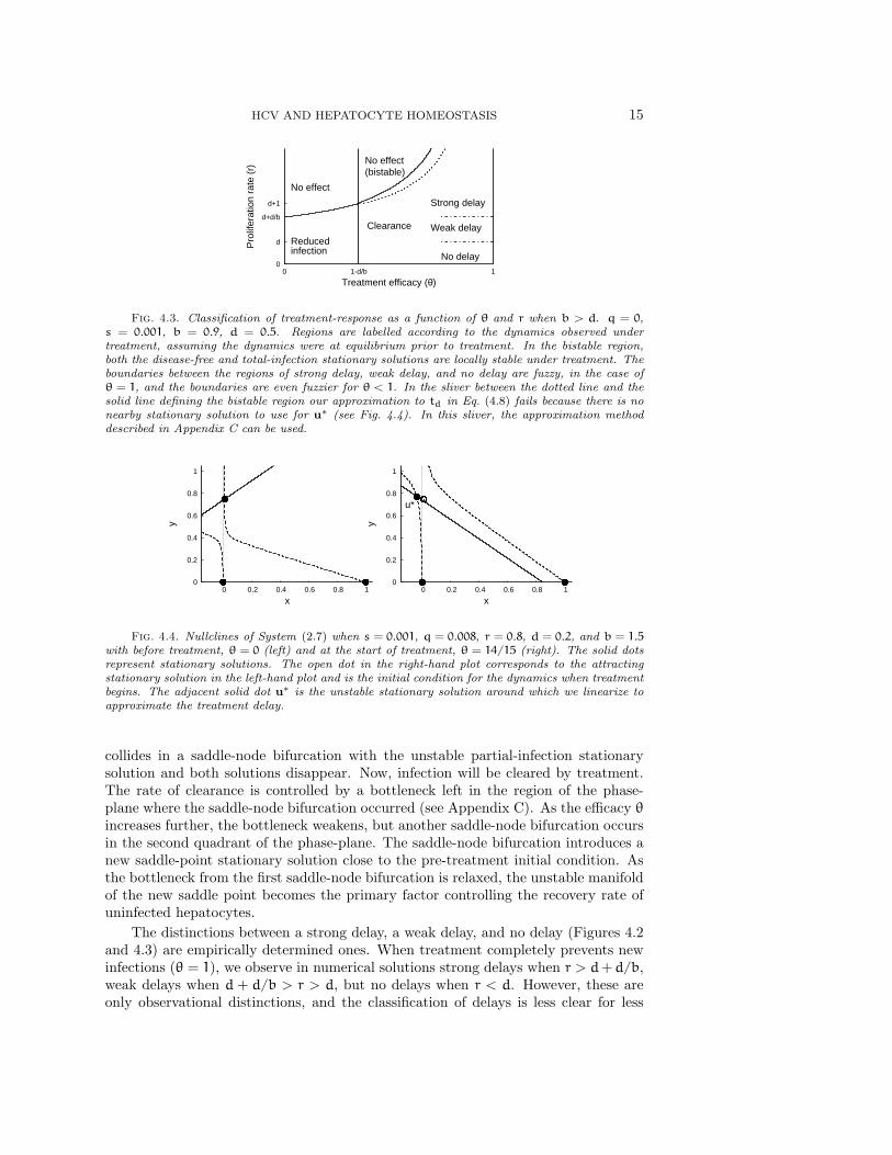
Fig. 4.3. Classification of treatment-response as a function of θ and r when b > d. q = 0,s = 0.001, b = 0.9, d = 0.5. Regions are labelled according to the dynamics observed undertreatment, assuming the dynamics were at equilibrium prior to treatment. In the bistable region,both the disease-free and total-infection stationary solutions are locally stable under treatment. Theboundaries between the regions of strong delay, weak delay, and no delay are fuzzy, in the case ofθ = 1, and the boundaries are even fuzzier for θ < 1. In the sliver between the dotted line and thesolid line defining the bistable region our approximation to td in Eq. (4.8) fails because there is nonearby stationary solution to use for u∗ (see Fig. 4.4). In this sliver, the approximation methoddescribed in Appendix C can be used.

0

0.2

0.4

0.6

0.8

1

0 0.2 0.4 0.6 0.8 1

y

x

0

0.2

0.4

0.6

0.8

1

0 0.2 0.4 0.6 0.8 1

y

x

u*

Fig. 4.4. Nullclines of System (2.7) when s = 0.001, q = 0.008, r = 0.8, d = 0.2, and b = 1.5with before treatment, θ = 0 (left) and at the start of treatment, θ = 14/15 (right). The solid dotsrepresent stationary solutions. The open dot in the right-hand plot corresponds to the attractingstationary solution in the left-hand plot and is the initial condition for the dynamics when treatmentbegins. The adjacent solid dot u∗ is the unstable stationary solution around which we linearize toapproximate the treatment delay.

collides in a saddle-node bifurcation with the unstable partial-infection stationarysolution and both solutions disappear. Now, infection will be cleared by treatment.The rate of clearance is controlled by a bottleneck left in the region of the phase-plane where the saddle-node bifurcation occurred (see Appendix C). As the efficacy θincreases further, the bottleneck weakens, but another saddle-node bifurcation occursin the second quadrant of the phase-plane. The saddle-node bifurcation introduces anew saddle-point stationary solution close to the pre-treatment initial condition. Asthe bottleneck from the first saddle-node bifurcation is relaxed, the unstable manifoldof the new saddle point becomes the primary factor controlling the recovery rate ofuninfected hepatocytes.

The distinctions between a strong delay, a weak delay, and no delay (Figures 4.2and 4.3) are empirically determined ones. When treatment completely prevents newinfections (θ = 1), we observe in numerical solutions strong delays when r > d+d/b,weak delays when d + d/b > r > d, but no delays when r < d. However, these areonly observational distinctions, and the classification of delays is less clear for less


efficient treatments.The existence of a treatment delay is most clean-cut in cases like that of Figure 4.4,

where almost all hepatocytes are infected before treatment and treatment is highlyeffective. We will now describe a method for approximating the dynamics at the startof treatment and determining the delay, td, before the number of infected hepatocytesbegins to decline in these cases. We can use the linearization of System (2.7) near thenew unstable stationary solution u∗ = (x∗, y∗) (Figure 4.4) given by the solutions of

0 =(1− θ)b (1+ (1− θ)b− r) (x∗)2

+ [(r(1− θ)b− d(1− θ)b− d) + q (r− 1− 2 (1− θ)b)] x∗ − sr− (r− d− q)q

(4.3a)

with y∗ =

((1− θ)b

r− 1

)x∗ + 1−

d+ q

r(4.3b)

that is nearest to the positive quadrant. In the neighborhood of u∗, the solution ofSystem (2.7) is approximately given by

u(t) = u∗ + eJ(u∗)t (u(0) − u∗) (4.4)

where u(0) is the pre-treatment equilibrium, and J(u∗) is the Jacobian matrix atu∗. The matrix exponential can be conveniently expressed in terms of the Lagrangeinterpolation formula [33]

eJt =

N∑n=1

eznt∏i6=n

(J − ziIzn − zi

), (4.5)

where zn is the n-th eigenvalue and I is the identity matrix. When s and q are small,u∗ = (x∗, y∗) ≈ (0, 1− d/r) (see Appendix A), so the Jacobian

J(u∗) ≈[

dr (1+ (1− θ)b) − (1− θ)b 0

((1− θ)b− r)(1− d

r

)d− r

]. (4.6)

The eigenvalues are approximately

d

r(1+ (1− θ)b) − (1− θ)b and d− r. (4.7)

Exact formulas can be obtained using the radical expressions for u∗ = (x∗, y∗).As the final part of the process of determining the treatment delay td, we have

to identify a condition that marks the end of a treatment delay and agrees withour intuitive observations. There are many possible choices (see Appendix B fora discussion). We found that the condition x(td) = y(td), corresponding to thepoint where the number of uninfected cells equals the number of infected cells, wassimple, convenient, and robust for calculating td over the strong-delay parameterrange. Solving for td, we find

td =r

d+ (1− θ)b(d− r)log{

[(r− (1− θ)b)(r− d) + d](y∗ − x∗)

[2(r− (1− θ)b)(r− d) + d](x(0) − x∗)

}. (4.8)

The dimensional delay time is td =td

rT − dTdays. A side-by-side comparison of

Eq. (4.8) to the actual value calculated by numerical solution of System (2.7) is shown


1

1.5

2

2.5

3

0.5 0.6 0.7 0.8 0.9 1

Pro

lifer

atio

n ra

te (

r)


Numerical Calculation of td

10

20

100∞

1

1.5

2

2.5

3

0.5 0.6 0.7 0.8 0.9 1


Linear Approximation of td

10

20

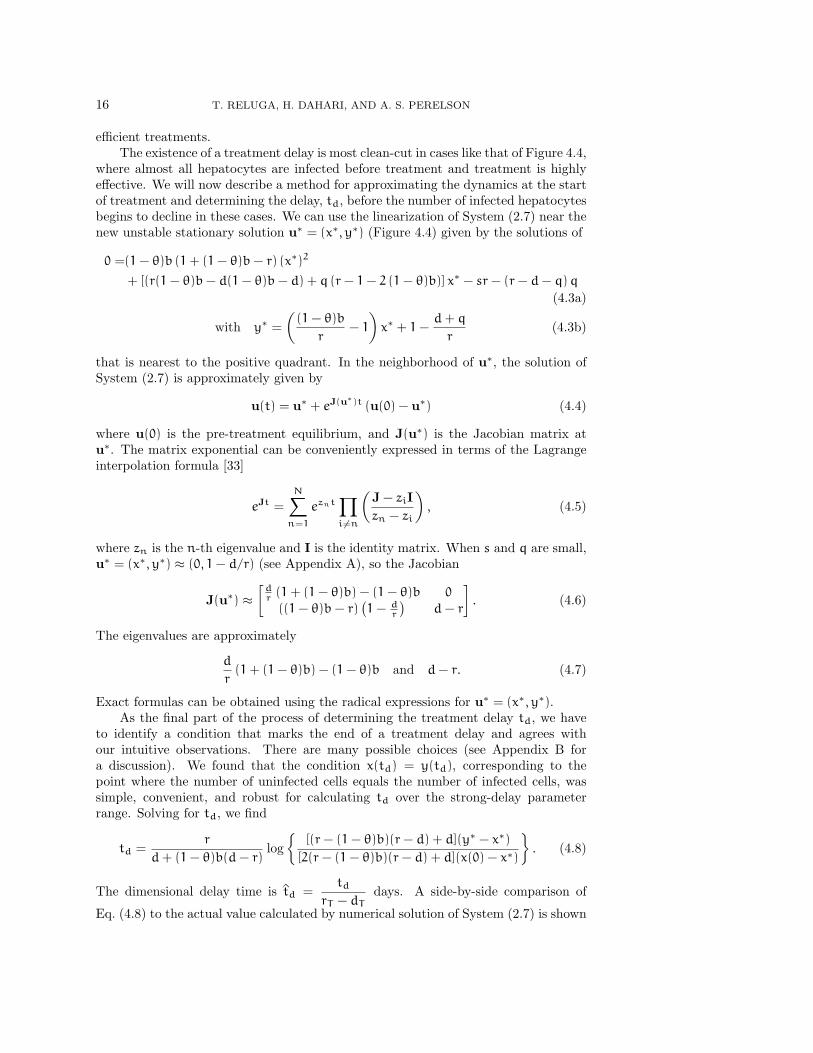
100∞

Fig. 4.5. Side-by-side comparison of contour plots of the treatment delay td using numericalsolution of System (2.7) (left) and the Formula (4.8) derived from the linear approximation (right).

The approximate bound on bistability, r = d+d

(1 − θ)b, labeled ∞, is the same in both plots. Contour

heights are 10, 20, 100, and ∞. Parameter values d = 0.5, b = 1, s = 10−3, q = 0. θc = 0.5 whenr = 0 in both plots.

10-2

10-1

100

10-2 10-1 100 101 102 103

Exc

ess

deat

h ra

te (

d)


100

50

20

10.1

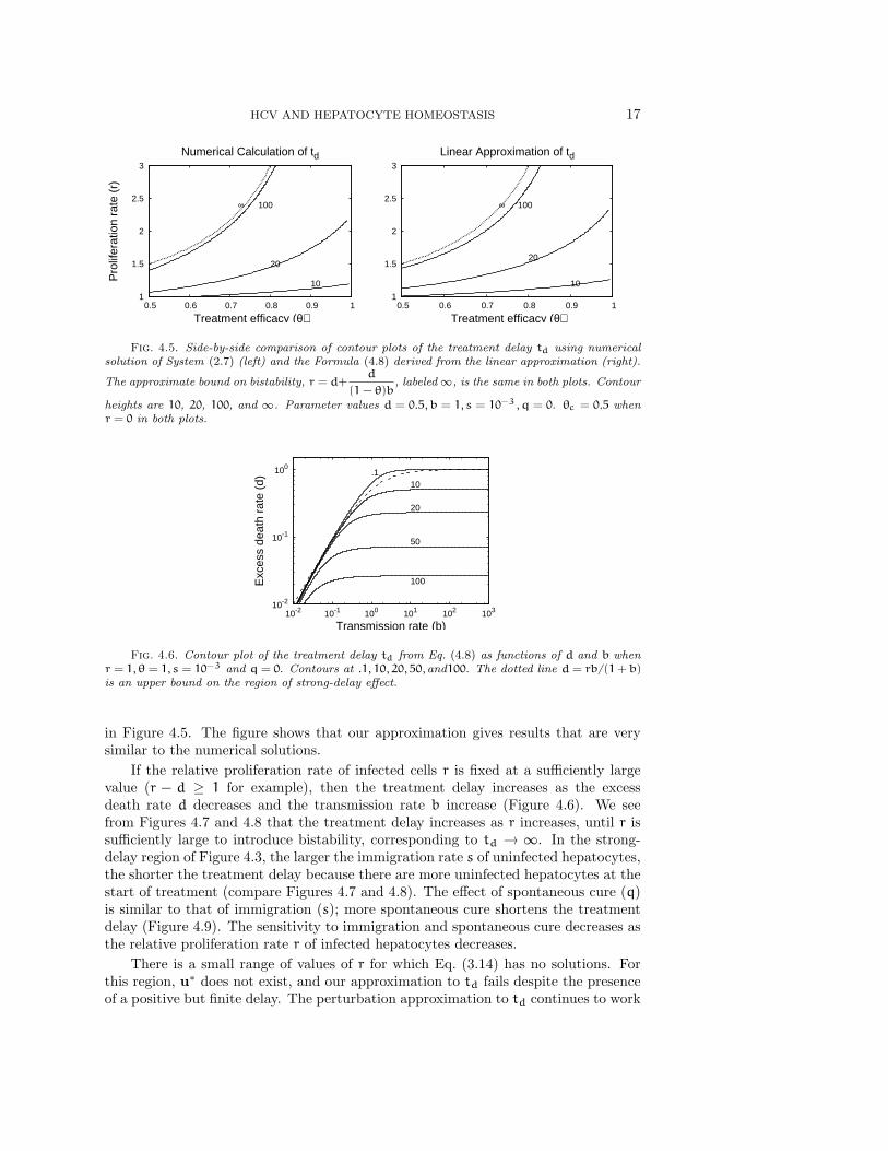
Fig. 4.6. Contour plot of the treatment delay td from Eq. (4.8) as functions of d and b whenr = 1, θ = 1, s = 10−3 and q = 0. Contours at .1, 10, 20, 50, and100. The dotted line d = rb/(1+ b)is an upper bound on the region of strong-delay effect.

in Figure 4.5. The figure shows that our approximation gives results that are verysimilar to the numerical solutions.

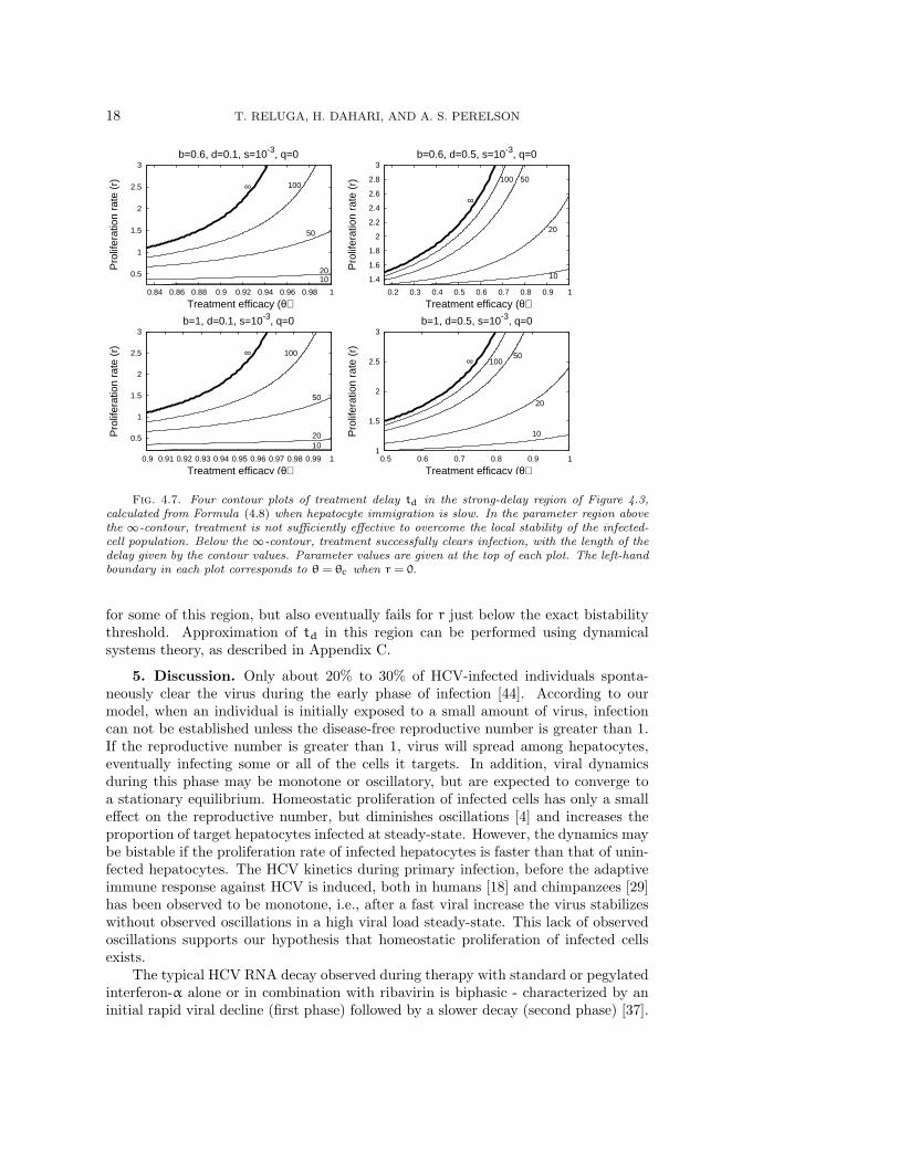
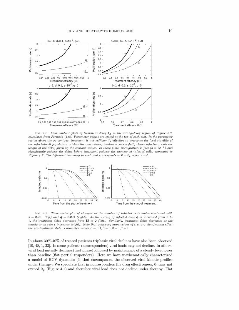
If the relative proliferation rate of infected cells r is fixed at a sufficiently largevalue (r − d ≥ 1 for example), then the treatment delay increases as the excessdeath rate d decreases and the transmission rate b increase (Figure 4.6). We seefrom Figures 4.7 and 4.8 that the treatment delay increases as r increases, until r issufficiently large to introduce bistability, corresponding to td → ∞. In the strong-delay region of Figure 4.3, the larger the immigration rate s of uninfected hepatocytes,the shorter the treatment delay because there are more uninfected hepatocytes at thestart of treatment (compare Figures 4.7 and 4.8). The effect of spontaneous cure (q)is similar to that of immigration (s); more spontaneous cure shortens the treatmentdelay (Figure 4.9). The sensitivity to immigration and spontaneous cure decreases asthe relative proliferation rate r of infected hepatocytes decreases.

There is a small range of values of r for which Eq. (3.14) has no solutions. Forthis region, u∗ does not exist, and our approximation to td fails despite the presenceof a positive but finite delay. The perturbation approximation to td continues to work


0.5

1

1.5

2

2.5

3

0.84 0.86 0.88 0.9 0.92 0.94 0.96 0.98 1

Pro

lifer

atio

n ra

te (

r)


b=0.6, d=0.1, s=10-3, q=0

1020

50

100∞

1.4

1.6

1.8

2

2.2

2.4

2.6

2.8

3

0.2 0.3 0.4 0.5 0.6 0.7 0.8 0.9 1

Pro

lifer

atio

n ra

te (

r)


b=0.6, d=0.5, s=10-3, q=0

10

20

50100

∞

0.5

1

1.5

2

2.5

3

0.9 0.91 0.92 0.93 0.94 0.95 0.96 0.97 0.98 0.99 1

Pro

lifer

atio

n ra

te (

r)


b=1, d=0.1, s=10-3, q=0

1020

50

100∞

1

1.5

2

2.5

3

0.5 0.6 0.7 0.8 0.9 1

Pro

lifer

atio

n ra

te (

r)


b=1, d=0.5, s=10-3, q=0

10

20

50100∞

Fig. 4.7. Four contour plots of treatment delay td in the strong-delay region of Figure 4.3,calculated from Formula (4.8) when hepatocyte immigration is slow. In the parameter region abovethe ∞-contour, treatment is not sufficiently effective to overcome the local stability of the infected-cell population. Below the ∞-contour, treatment successfully clears infection, with the length of thedelay given by the contour values. Parameter values are given at the top of each plot. The left-handboundary in each plot corresponds to θ = θc when r = 0.

for some of this region, but also eventually fails for r just below the exact bistabilitythreshold. Approximation of td in this region can be performed using dynamicalsystems theory, as described in Appendix C.

5. Discussion. Only about 20% to 30% of HCV-infected individuals sponta-neously clear the virus during the early phase of infection [44]. According to ourmodel, when an individual is initially exposed to a small amount of virus, infectioncan not be established unless the disease-free reproductive number is greater than 1.If the reproductive number is greater than 1, virus will spread among hepatocytes,eventually infecting some or all of the cells it targets. In addition, viral dynamicsduring this phase may be monotone or oscillatory, but are expected to converge toa stationary equilibrium. Homeostatic proliferation of infected cells has only a smalleffect on the reproductive number, but diminishes oscillations [4] and increases theproportion of target hepatocytes infected at steady-state. However, the dynamics maybe bistable if the proliferation rate of infected hepatocytes is faster than that of unin-fected hepatocytes. The HCV kinetics during primary infection, before the adaptiveimmune response against HCV is induced, both in humans [18] and chimpanzees [29]has been observed to be monotone, i.e., after a fast viral increase the virus stabilizeswithout observed oscillations in a high viral load steady-state. This lack of observedoscillations supports our hypothesis that homeostatic proliferation of infected cellsexists.

The typical HCV RNA decay observed during therapy with standard or pegylatedinterferon-α alone or in combination with ribavirin is biphasic - characterized by aninitial rapid viral decline (first phase) followed by a slower decay (second phase) [37].


0.5

1

1.5

2

2.5

3

0.84 0.86 0.88 0.9 0.92 0.94 0.96 0.98 1

Pro

lifer

atio

n ra

te (

r)


b=0.6, d=0.1, s=10-2, q=0

10

20

∞

1.4

1.6

1.8

2

2.2

2.4

2.6

2.8

3

0.2 0.3 0.4 0.5 0.6 0.7 0.8 0.9 1

Pro

lifer

atio

n ra

te (

r)


b=0.6, d=0.5, s=10-2, q=0

10

20

∞

0.5

1

1.5

2

2.5

3

0.9 0.91 0.92 0.93 0.94 0.95 0.96 0.97 0.98 0.99 1

Pro

lifer

atio

n ra

te (

r)


b=1, d=0.1, s=10-2, q=0

10

20

∞

1

1.5

2

2.5

3

0.5 0.6 0.7 0.8 0.9 1

Pro

lifer

atio

n ra

te (

r)


b=1, d=0.5, s=10-2, q=0

10

20

∞

Fig. 4.8. Four contour plots of treatment delay td in the strong-delay region of Figure 4.3,calculated from Formula (4.8). Parameter values are stated at the top of each plot. In the parameterregion above the ∞-contour, treatment is not sufficiently effective to overcome the local stability ofthe infected-cell population. Below the ∞-contour, treatment successfully clears infection, with thelength of the delay given by the contour values. In these plots, immigration is fast (s = 10−2) andsignificantly reduces the delay before treatment reduces the number of infected cells, compared toFigure 4.7. The left-hand boundary in each plot corresponds to θ = θc when r = 0.

0.001

0.01

0.1

1

-5 0 5 10 15 20 25 30 35 40

Infe

cted

cel

ls (

y)

Time from the start of treatment

q=0q=0.001q=0.01q=0.1q=1

0.001

0.01

0.1

1

-5 0 5 10 15 20 25 30 35 40

Infe

cted

cel

ls (

y)

Time from the start of treatment

s=0s=0.001s=0.01s=0.1s=1

Fig. 4.9. Time series plot of changes in the number of infected cells under treatment withs = 0.001 (left) and q = 0.001 (right). As the curing of infected cells q is increased from 0 to1, the treatment delay decreases from 15 to 0 (left). Similarly, treatment delay decreases as theimmigration rate s increases (right). Note that only vary large values of s and q significantly effectthe pre-treatment state. Parameter values d = 0.3, b = 3, θ = 1, r = 1.

In about 30%-40% of treated patients triphasic viral declines have also been observed[19, 48, 1, 23]. In some patients (nonresponders) viral loads may not decline. In others,viral load initially declines (first phase) followed by maintenance of a steady level lowerthan baseline (flat partial responders). Here we have mathematically characterizeda model of HCV dynamics [6] that encompasses the observed viral kinetic profilesunder therapy. We speculate that in nonresponders the drug effectiveness, θ, may notexceed θp (Figure 4.1) and therefore viral load does not decline under therapy. Flat


partial responders may be explained as a consequence of drug efficacy higher than θp

but lower than the critical drug efficacy θc (Figure 4.1). Viral clearance occurs whenθ > θc via biphasic or triphasic viral decline when the hepatocyte proliferation rate,r, is lower or higher than the hepatocyte death rate, d, respectively (System (2.7)without “cure”; Figure 4.1).

Using perturbation theory, we showed a delay can occur between the start of treat-ment and the first measurable decline in the number of infected hepatocytes underefficient therapy (θ > θc) because of the influence of a near-by saddle-node bifurcationin the system (Figure 4.4). Equation (4.8) can be used to approximate the durationof this delay. In terms of viral dynamics, this delay appears as a shoulder phase sep-arating the initial decay in viral load at the start of treatment from the asymptoticclearance phase. One of the conditions for the existence of this delay between theinitial decrease and asymptotic clearance is that the number of infected cells is muchlarger than the number of uninfected cells at the start of therapy. During therapythe number of uninfected cells increases. Because of density-dependent homeostaticprocesses, the proliferation of infected cells slows as the number of uninfected cellsincreases. When this proliferation slows to the point at which it no longer keeps upwith the rate of infected cell loss, the number of infected cells start to decline. Theshoulder persists until the ratio between uninfected cells and infected cells is approx-imately one. We found that the stopping condition, T/I ≈ 1, for calculating whenthe shoulder phase ends, is simple and robust for calculating td over a large-shoulderparameter range. Other topping conditions T/I ≈ 1 are discussed in Appendix B.

When using td in the context of the full model (System (2.1)), i.e., calculatingthe viral shoulder phase and hence a triphasic viral decay, our formula (Eq. (4.8)) hasto be adjusted. Since interferon-α mainly inhibits viral production, and we assumethat initially the infected cell number remains close to its level before therapy, thenthe model (System (2.1)) predicts that viral load will decline from its baseline value,V0, according to the equation: V(t) = V0 (1− ε+ εe−ct)[37]. This equation for thefirst phase of viral decline predicts that at times long compared with 1/c, the averagefree virion lifetime in serum, the viral load will decline to (1 − ε)V0 over an intervalof length ln(1 − ε)/c (Fig. 2.1). Therefore, our formula (Eq. (4.8)), which estimatesthe length of time since the start of therapy and the beginning of the third phase ofdecline (Fig. 2.1 right panel) can be adjusted to the actual viral shoulder duration bysubtracting the relaxation time ln(1− ε)/c from the dimensional form of td.

We have previously predicted, using System (2.1), that the spontaneous curing(q) of infected cells by a noncytolytic immune response is necessary to prevent asignificant loss of liver cells during acute HCV infection in chimpanzees [5]. Directevidence for noncytolytic clearance of HCV from infected cells has not yet been found,but interferon-α has cured replicon cells [2] and clearance of hepatitis-B-virus-infectedhepatocytes has been shown to occur through noncytolytic mechanisms [16]. In thecontext of treatment in chronic-HCV patients, our theory predicts that any shoulderphase will be shortened by a strong noncytolytic response.

HCV is the only known RNA virus with an exclusively cytoplasmic life cycle thatis associated with cancer [47]. The mechanisms by which it causes cancer are unclear.It may be possible that the path to hepatocellular carcinoma in chronic hepatitis Cshares some important features with human papillomavirus-induced carcinogenesis[17]. Interactions of HCV proteins with key regulators of the cell cycle, e.g., theretinoblastoma protein [34] and p53 [22], may lead to enhanced cellular proliferationover uninfected cells and may also compromise multiple cell cycle checkpoints that


act to maintain genomic integrity [11], thus setting the stage for carcinogenesis. Inlight of these speculations, the proliferation of HCV-infected cells, rI, may be higherthan proliferation of uninfected cells, rT . Therefore, in this study we also analyzedthis assumption (i.e., rI > rT ). We found that when rI > rT bistability arises (undercertain parameter values), and imposing rI < rT is sufficient to preclude bistability.However, more experimental work is needed to test the consistency of this view ofhomeostatic proliferation with the behavior of hepatocytes in vivo. Our model makessome predictions regarding changes in the total hepatocyte numbers over the courseof infection and treatment. Since liver function is correlated to hepatocyte numbers,the total number of hepatocytes may be an important medical indicator and mayfurther inform our understanding of HCV.

On a mathematical note, there is as yet no global stability analysis of System (2.1).Of particular importance, a closer analysis of the quasi-steady state approximationis needed. This is emphasized by numerical observations that a Hopf bifurcation ofthe partial-infection stationary solution can occur if the viral clearance rate c is notsufficiently large. Applications and extension of methods from De Leenheer and Smith[9], De Leenheer and Pilyugin [8] and Korobeinikov [24] may prove useful in furtherwork.

The analyses presented here are important not only for HCV infection but shouldalso be relevant for modeling other infections with hepatotropic viruses, such as hep-atitis B virus. Many mathematical models for the study of hepatitis B virus DNAkinetics under therapy ignore the proliferation of virus-infected cells [36]. Interest-ingly, besides the typical biphasic decay in viral load, other kinetic profiles have beenobserved, such as triphasic. As our model allows one to predict more complex viraldecay profiles, we hope that it will be useful for understanding complex HCV andHBV kinetics under therapy [7].

6. Acknowledgements. T. Reluga thanks A. Zilman for helpful discussion con-cerning the calculations in Appendix C.

References.[1] F. C. Bekkering, A. U. Neumann, J. T. Brouwer, R. S. Levi-Drummer,

and S. W. Schalm, Changes in anti-viral effectiveness of interferon after dosereduction in chronic hepatitis C patients: A case control study, BMC Gastroen-terology, 1 (2001), p. 14.

[2] K. J. Blight, J. A. McKeating, and C. M. Rice, Highly permissive celllines for subgenomic and genomic hepatitis C virus RNA replication, Journal ofVirology, 76 (2002), pp. 13001–13014.

[3] H. Dahari, A. Feliu, M. Garcia-Retortillo, X. Forns, and A. U. Neu-mann, Second hepatitis C replication compartment indicated by viral dynamicsduring liver transplantation, Journal of Hepatology, 42 (2005), pp. 491–498.

[4] H. Dahari, A. Lo, R. M. Ribeiro, and A. S. Perelson, Modeling hepati-tis C virus dynamics: Liver regeneration and critical drug efficacy, Journal ofTheoretical Biology, 47 (2007), pp. 371–381.

[5] H. Dahari, M. Major, X. Zhang, K. Mihalik, C. M. Rice, A. S. Perel-son, S. M. Feinstone, and A. U. Neumann, Mathematical modeling of pri-mary hepatitis C infection: Noncytolytic clearance and early blockage of virionproduction, Gastroenterology, 128 (2005), pp. 1056–1066.

[6] H. Dahari, R. M. Ribeiro, and A. S. Perelson, Triphasic decline of HCVRNA during antiviral therapy, Hepatology, 46 (2007), pp. 16–21.


[7] H. Dahari, E. Shudo, R. M. Ribeiro, and A. S. Perelson, Modeling com-plex decay profiles of hepatitis B virus during antiviral therapy, Hepatolgy (inpress).

[8] P. De Leenheer and S. Pilyugin, Multi-strain virus dynamics with mutations:A global analysis, Arxiv preprint arXiv:0707.4501.

[9] P. De Leenheer and H. Smith, Virus Dynamics: A Global Analysis, SIAMJournal on Applied Mathematics, 63 (2003), pp. 1313–1327.

[10] G. Di Liberto and C. Feray, The anhepatic phase of liver transplantation asa model for measuring the extra-hepatic replication of hepatitis C virus, Journalof Hepatology, 42 (2005), pp. 441–443.

[11] S. Duensing and K. Munger, Mechanisms of genomic instability in humancancer: Insights from studies with human papillomavirus oncoproteins, Interna-tional Journal of Cancer, 109 (2004), pp. 157–162.

[12] N. Fausto, Liver regeneration and repair: hepatocytes, progenitor cells, andstem cells, Hepatology, 39 (2004), pp. 1477–1487.

[13] M. W. Fried, M. L. Shiffman, K. R. Reddy, C. Smith, G. Marinos,F. L. Goncales, D. Haussinger, M. Diago, G. Carosi, D. Dhumeaux,A. Carxi, A. Lin, J. Hoffman, and J. Yu, Peginterferon alfa-2a plus ribavirinfor chronic hepatitis C virus infection, New England Journal of Medicine, 347(2002), pp. 975–982.

[14] H. Gomez-Acevedo and M. Y. Li, Backward bifurcation in a model for HTLV-I infection of CD4+ T cells, Bulletin of Mathematical Biology, 67 (2005), pp.101–114.

[15] J. Guckenheimer and P. Holmes, Nonlinear Oscillations, Dynamical Sys-tems, and Bifurcations of Vector Fields, Springer, New York, NY (1983).

[16] L. G. Guidotti, R. Rochford, J. Chung, M. Shapiro, R. Purcell, andF. V. Chisari, Viral clearance without destruction of infected cells during acuteHBV infection, Science, 284 (1999), p. 825.

[17] C. M. Hebner and L. A. Laimins, Human papillomaviruses: basic mechanismsof pathogenesis and oncogenicity, Reviews in Medical Virology, 16 (2006), pp. 83–97.

[18] B. L. Herring, R. Tsui, L. Peddada, M. Busch, and E. L. Delwart,Wide range of quasispecies diversity during primary hepatitis C virus infection,Journal of Virology, 79 (2005), pp. 4340–4346.

[19] E. Herrmann, J. Lee, G. Marinos, M. Modi, and S. Zeuzem, Effect ofribavirin on hepatitis C viral kinetics in patients treated with pegylated interferon,Hepatology, 37 (2003), pp. 1351–1358.

[20] J. Hofbauer and K. Sigmund, Evolutionary Games and Population Dynam-ics, Cambridge University Press, Cambridge, UK (1998).

[21] G. E. Hutchinson, An Introduction to Population Ecology, Yale UniversityPress, New Haven, CT (1978).

[22] C. F. Kao, S. Y. Chen, J. Y. Chen, and Y. H. W. Lee, Modulation of p53transcription regulatory activity and post-translational modification by hepatitisC virus core protein, Oncogene, 23 (2004), pp. 2472–2483.

[23] T. L. Kieffer, C. Sarrazin, J. S. Miller, M. W. Welker, N. Forestier,A. D. Kwong, and S. Zeuzem, Telaprevir and pegylated interferon-alpha-2ainhibit wild-type and resistant genotype 1 hepatitis C virus replication in patients.,Hepatology, 46 (2007), pp. 631–639.

[24] A. Korobeinikov, Global properties of basic virus dynamics models, Bulletin of


Mathematical Biology, 66 (2004), pp. 879–883.[25] B. D. Lindenbach and C. M. Rice, Unravelling hepatitis C virus replication

from genome to function, Nature, 436 (2005), pp. 933–938.[26] R. A. Macdonald, “Lifespan” of liver cells. Autoradio-graphic study using tri-

tiated thymidine in normal, cirrhotic, and partially hepatectomized rats, Archivesof Internal Medicine, 107 (1961), pp. 335–343.

[27] I. R. Mackay, Hepatoimmunology: A perspective. Special Feature, Immunologyand Cell Biology, 80 (2002), pp. 36–44.

[28] R. N. M. Macsween, A. D. Burt, B. C. Portmann, K. G. Ishak, P. J.Scheuer, and P. P. Anthony, Pathology of the Liver, Churchill Livingstone(1987).

[29] M. E. Major, H. Dahari, K. Mihalik, M. Puig, C. M. Rice, A. U.Neumann, and S. M. Feinstone, Hepatitis C virus kinetics and host responsesassociated with disease and outcome of infection in chimpanzees, Hepatology, 39(2004), pp. 1709–1720.

[30] M. P. Manns, J. G. McHutchison, S. C. Gordon, V. K. Rustgi,M. Shiffman, R. Reindollar, Z. D. Goodman, K. Koury, M. H. Ling,and J. K. Albrecht, Peginterferon alfa-2b+ ribavirin compared with interferonalfa-2b+ ribavirin for initial treatment of chronic hepatitis C: a randomised trial,The Lancet, 358 (2001), pp. 958–965.

[31] P. Meuleman, L. Libbrecht, R. De Vos, B. de Hemptinne, K. Gevaert,J. Vandekerckhove, T. Roskams, and G. Leroux-Roels, Morphologi-cal and biochemical characterization of a human liver in a uPA-SCID mousechimera, Hepatology, 41 (2005), pp. 847–856.

[32] G. K. Michalopoulos and M. C. DeFrances, Liver regeneration, Science,276 (1997), pp. 60–66.

[33] C. Moler and C. V. Loan, Nineteen dubious ways to compute the exponentialof a matrix, twenty-five years later, SIAM Review, 45 (2003), pp. 3–49.

[34] T. Munakata, M. Nakamura, Y. Liang, K. Li, and S. M. Lemon, Down-regulation of the retinoblastoma tumor suppressor by the hepatitis C virus NS5BRNA-dependent RNA polymerase, Proceedings of the National Academy of Sci-ences, 102 (2005), pp. 18159–18164.

[35] J. D. Murray, Mathematical Biology, 2nd ed., Springer, New York, NY (1993).[36] A. U. Neumann, Hepatitis B viral kinetics: A dynamic puzzle still to be resolved,

Hepatology, 42 (2005), pp. 249–54.[37] A. U. Neumann, N. P. Lam, H. Dahari, D. R. Gretch, T. E. Wiley,

T. J. Layden, and A. S. Perelson, Hepatitis C viral dynamics in vivo andthe antiviral efficacy of interferon-alpha therapy, Science, 282 (1998), pp. 103–107.

[38] NIH, National institutes of health consensus development conference: manage-ment of hepatitis C, Hepatology, 36 (2002), pp. S3–20.

[39] I. M. Pedersen, G. Cheng, S. Wieland, S. Volinia, C. M. Croce, F. V.Chisari, and M. David, Interferon modulation of cellular microRNAs as anantiviral mechanism, Nature, 449 (2007), pp. 919–922.

[40] A. Perelson, A. Neumann, M. Markowitz, J. Leonard, and D. Ho,HIV-1 dynamics in vivo: virion clearance rate, infected cell life-span, and viralgeneration time, Science, 271 (1996), pp. 1582–1586.

[41] A. S. Perelson, Modelling viral and immune system dynamics, Nature ReviewsImmunology, 2 (2002), pp. 28–36.


[42] A. S. Perelson, E. Herrmann, F. Micol, and S. Zeuzem, New kineticmodels for the hepatitis C virus, Hepatology, 42 (2005), pp. 749–754.

[43] K. A. Powers, R. M. Ribeiro, K. Patel, S. Pianko, L. Nyberg, P. Pock-ros, A. J. Conrad, J. McHutchison, and A. S. Perelson, Kinetics ofhepatitis C virus reinfection after liver transplantation, Liver Transplantation,12 (2006), pp. 207–216.

[44] B. Rehermann and M. Nascimbeni, Immunology of hepatitis B virus andhepatitis C virus infection, Nature Reviews Immunology, 5 (2005), pp. 215–229.

[45] R. Ribeiro, Dynamics of alanine aminotransferase during hepatitis C virustreatment, Hepatology, 38 (2003), pp. 509–517.

[46] L. B. Seeff, Natural history of chronic hepatitis C, Hepatology, 36 (2002), pp.S35–S46.

[47] L. B. Seeff and J. H. Hoofnagle, Epidemiology of hepatocellular carcinomain areas of low hepatitis B and hepatitis C endemicity, Oncogene, 25 (2006), pp.3771–3777.

[48] R. E. Sentjens, C. J. Weegink, M. G. Beld, M. C. Cooreman, andH. W. Reesink, Viral kinetics of hepatitis C virus RNA in patients with chronichepatitis C treated with 18 MU of interferon alpha daily, European journal ofgastroenterology and hepatology, 14 (2002), pp. 833–840.

[49] S. Sherlock and J. Dooley, Diseases of the Liver and Biliary System, Black-well Science (2002).

[50] N. D. Theise, M. Nimmakayalu, R. Gardner, P. B. Illei, G. Morgan,L. Teperman, O. Henegariu, and D. S. Krause, Liver from bone marrowin humans, Hepatology, 32 (2000), pp. 11–16.

[51] R. Thimme, D. Oldach, K. M. Chang, C. Steiger, S. C. Ray, and F. V.Chisari, Determinants of viral clearance and persistence during acute hepatitisC virus infection, Journal of Experimental Medicine, 194 (2001), pp. 1395–1406.

[52] X. Wei, S. Ghosh, M. Taylor, V. Johnson, E. Emini, P. Deutsch, J. Lif-son, S. Bonhoeffer, M. Nowak, B. Hahn, et al., Viral dynamics in humanimmunodeficiency virus type 1 infection, Nature, 373 (1995), pp. 117–122.

Appendix A. Perturbation Approximations.Regular perturbation methods can be used to approximate the stationary solu-

tions of System (2.7) in the limits of small s and q, based on the polynomials inEq. (3.11) and Eq. (3.14a). Eq. (3.11) is independent of q, so let x = x0 + sxs + o(s).Substituting into Eq. (3.11), (x0 + sxs)

2 − (x0 + sxs) = s, Collecting like terms,

x0(x0 − 1) − (1− 2x0xs + xs)s+ o(s) = 0. (A.1)

From the zeroth-order term in s, x0 ∈ {0, 1}, and to first order, xs = 12x0−1 . Thus,

the two corresponding stationary solutions for small s and q are

(−s+ o(s), 0) and (1+ s+ o(s), 0). (A.2)

Eq. (3.14a) depends on both s and q, so let x = x0 +sxs +qxq +o(s, q). Substitutinginto Eq. (3.14a) and collecting like terms,

0 = b(1+ b− r)x20 + (rb− db− d)x0

− (−xsrb+ xsdb+ xsd− 2bx0xs − 2b2x0xs + 2bx0xsr+ r)s

− (−bxqr+ xqdb+ xqd− x0r+ x0 + 2x0b− 2(1+ b+ r)bx0xq + r− d)q (A.3)


To highest order,

x0 ∈{0,d+ db− rb

b(1+ b− r)

}. (A.4)

The first order corrections in s and q are

xs =r

2x0b+ 2b2x0 − 2bx0r− d− bd+ br, (A.5a)

xq =r− x0r+ x0 + 2x0b− d

2x0b+ 2b2x0 − 2bx0r− d− bd+ br. (A.5b)

Eq. (3.14b) can then be used to determine y. In the special case of x0 = 0, thestationary solution is given by Eq. (3.15). This can be used to approximate both thepre-treatment and post-treatment (substituting (1 − θ)b for b) stationary solutionswhen applying Eq. (4.8).

Appendix B. Choosing a treatment delay threshold.Using Equation (4.4), we can approximate the delay, td, before the number of

infected hepatocytes begins to decline. But to do this, we have to find a quantitativerule for determining the end of the treatment delay. One way to do this is to choose aline, represented by a vector k and a constant k0, such that the shoulder ends whenthe approximate solution intersects this line. Thus, td is defined such that

kTu(td) = k0. (B.1)

Since we are concerned only with the divergence from steady-state, we can ignore thestable mode of Eq. (4.4), and Eq. B.1 leads to the formula

td =r

d+ (1− θ)b(d− r)log{

[(r− (1− θ)b)(r− d) + d](k1u∗1 + k2u∗2 − k0)

[(k1 − k2)(r− (1− θ)b)(r− d) + k1d](u∗1 − u1(0))

}(B.2)

Several choices for k and k0 are summarized in Table B.1, along with their draw-backs. The unstable manifold of u∗ has the initial direction[

d− (r− d)((1− θ)b− r), (r− d)((1− θ)b− r)]. (B.3)

If we constrain the application of Eq. (B.2) to the region of Figure 4.3 where θ > θc

and r > d, we can show that the choice of k = [1,−1], k0 = 0 always gives a solutionfor td. This is because the first component of the eigenvector is positive and thesecond is negative, ensuring that the orbit approximated by a line in the direction ofthe eigenvector will always intersect the line y = x. Numerical evidence indicates thatthis choice is reasonably consistent with the qualitative character of delays, and wewill use it throughout this paper. However, it underestimates the delay time in caseswhere r−d is small. In such situations, k = [1, 1], k0 = 1 gives better approximationsto td.

Appendix C. Bottle neck calculations.When the growth rate r is slightly smaller than the critical value r∗ that introduces

bistability (Figure 4.3), Equation (4.4) can not be used to estimate the treatment delaytd because there is no near-by equilibrium around-which we can linearize. However,we can still approximate the treatment delay by transforming the system near the


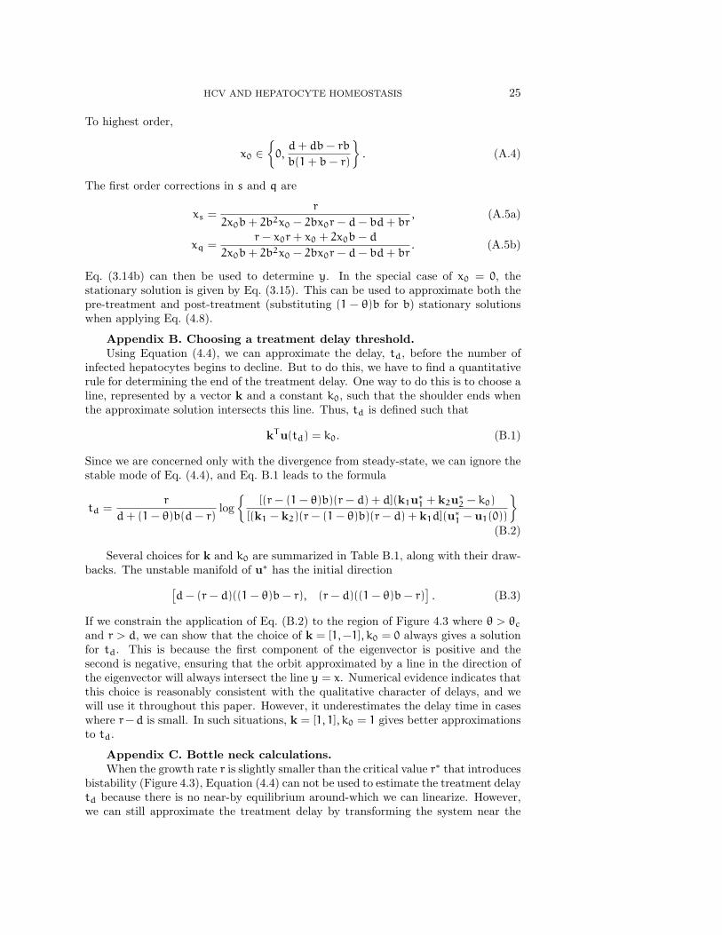
Table B.1Possible stopping condition choices for calculation of td.

Description k k0 CommentUpper bound [1, 1] 1 u(t) may not intersectx(t) = y(t) [1,−1] 0 u(t) may not intersect90% threshold [0, 1] .9 (1− d/r) u(t) may not intersect

Uninfected cells only [1, 0]d

rtd → 0 as d→ 0, although the delay may not

Uninfected cells only [1, 0] .1 may not correspond to the full delay

bifurcation point into normal form [15]. The normal form of a generic saddle-nodebifurcation satisfies the first-order differential equation

u = a0(r∗ − r) + a2u2 (C.1)

where r is the bifurcation parameter, and r = r∗ is the bifurcation point with a0 > 0

and a2 6= 0. Using elementary integration methods, we can show that for r ≈ r∗, thetime it takes for a solution to pass from a negative initial position to a positive finalposition, both far from the origin, is approximately given by

td ≈√π2/[a0a2(r∗ − r)]. (C.2)

As r is increased toward r∗, the time becomes longer. If r > r∗, the time is infinitebecause solutions are trapped by an intermediate attracting state. For this HCVmodel, our task to calculate r∗, a0, and a2 by transforming System (2.7) into normal-form near the saddle-node bifurcation that introduces bistability.

We can determine the bifurcation point r∗ by setting the discriminant of x inEquation (3.14a) (with transmission rate (1 − θ)b instead of b) equal to zero. Theresult is a quadratic polynomial for r∗, where the smaller solution corresponds to asaddle-node bifurcation for non-biological values of x, and the larger solution corre-sponds to bifurcation which is biologically important.

Once r∗ is known, we calculate the feasible non-hyperbolic equilibrium solution(x∗(r∗), y∗(r∗)) using Eq. (3.14). and transform System (2.7) using a change of vari-ables of the form

x = x∗ +Mxuu+Mxvv+Mxr(r− r∗), (C.3a)y = y∗ +Myuu+Myvv+Myr(r− r∗), (C.3b)

such that locally, the system has the form

u = a0(r∗ − r) + a2u2 + o(r∗ − r, u2) +O(v), (C.4a)

v = −a3v+ o(v), (C.4b)

where a0 and a2 satisfy the conditions given above and a3 > 0. This transformationcan be perform using the eigenvalue decomposition of the Jacobian at the equilibriumpoint, and then chosing Mxr and Myr to eliminate extra terms in u and v. TheO(v) terms are neglected because v converges to 0 exponentially near the bifurcation.The procedure is easily implemented numerically, but we have not produced a simpleanalytic formula for the result.

Documents

analysis of hepatitis c virus infection models with hepatocyte