Analysis of variance filevariance in two distinct ways: ... The results of computations of ANOVA methods are usually tabulated. The rows of such tables give the source of the variance;

Analysis of variance

1

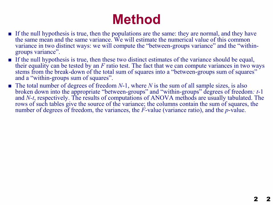
Method If the null hypothesis is true, then the populations are the same: they are normal, and they have

the same mean and the same variance. We will estimate the numerical value of this common variance in two distinct ways: we will compute the “between-groups variance” and the “within-groups variance”.

If the null hypothesis is true, then these two distinct estimates of the variance should be equal, their equality can be tested by an F ratio test. The fact that we can compute variances in two ways stems from the break-down of the total sum of squares into a “between-groups sum of squares” and a “within-groups sum of squares”.

The total number of degrees of freedom N-1, where N is the sum of all sample sizes, is also broken down into the appropriate “between-groups” and “within-groups” degrees of freedom: t-1 and N-t, respectively. The results of computations of ANOVA methods are usually tabulated. The rows of such tables give the source of the variance; the columns contain the sum of squares, the number of degrees of freedom, the variances, the F-value (variance ratio), and the p-value.

2HUSRB/0901/221/088 „Teaching Mathematics and Statistics in Sciences: Modeling and Computer-aided Approach 2

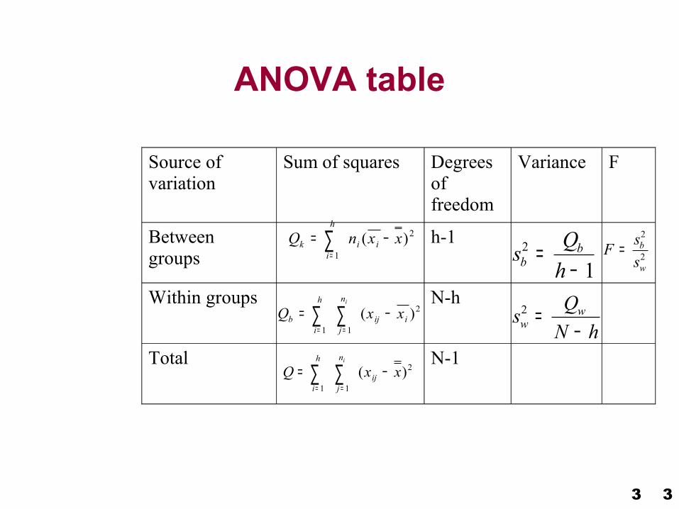
ANOVA table

Q n x xki

h

i i= −=

∑1

2( )s Q

hbb2

1=

−F s

sb

w

=2

2

Q x xbi

h

j

n

ij i

i

= −= =

∑ ∑1 1

2( ) s QN hw

w2 =−

Q x xi

h

j

n

ij

i

= −= =

∑ ∑1 1

2( )

Source of variation

Sum of squares Degrees of freedom

Variance F

Between groups

h-1

Within groups N-h

Total N-1


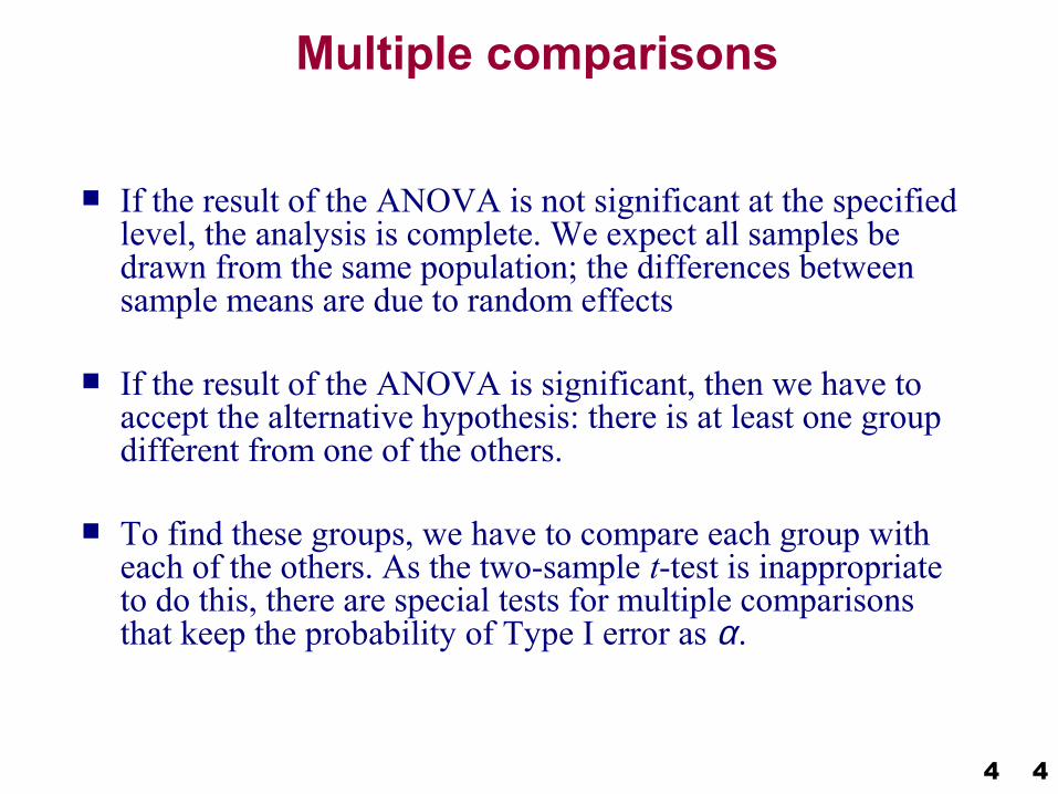
Multiple comparisons

If the result of the ANOVA is not significant at the specified level, the analysis is complete. We expect all samples be drawn from the same population; the differences between sample means are due to random effects

If the result of the ANOVA is significant, then we have to accept the alternative hypothesis: there is at least one group different from one of the others.

To find these groups, we have to compare each group with each of the others. As the two-sample t-test is inappropriate to do this, there are special tests for multiple comparisons that keep the probability of Type I error as α.


Pairwise methods I. The most often used multiple comparisons are the modified t-

tests. Another often used method is the so-called Bonferroni method: to achieve a level of not more than α for a set of a number of c tests, we need to choose a level α /c for the individual tests.

For example for three comparisons a p-value less than 0.05/3=0.017 has to be considered significant instead of p=0.05. This method is conservative. We know only that the probability does not exceed α for the set. This method can be used in cases involving small numbers of comparisons.

t x x

sn n

i j

bi j

= −

+1 1


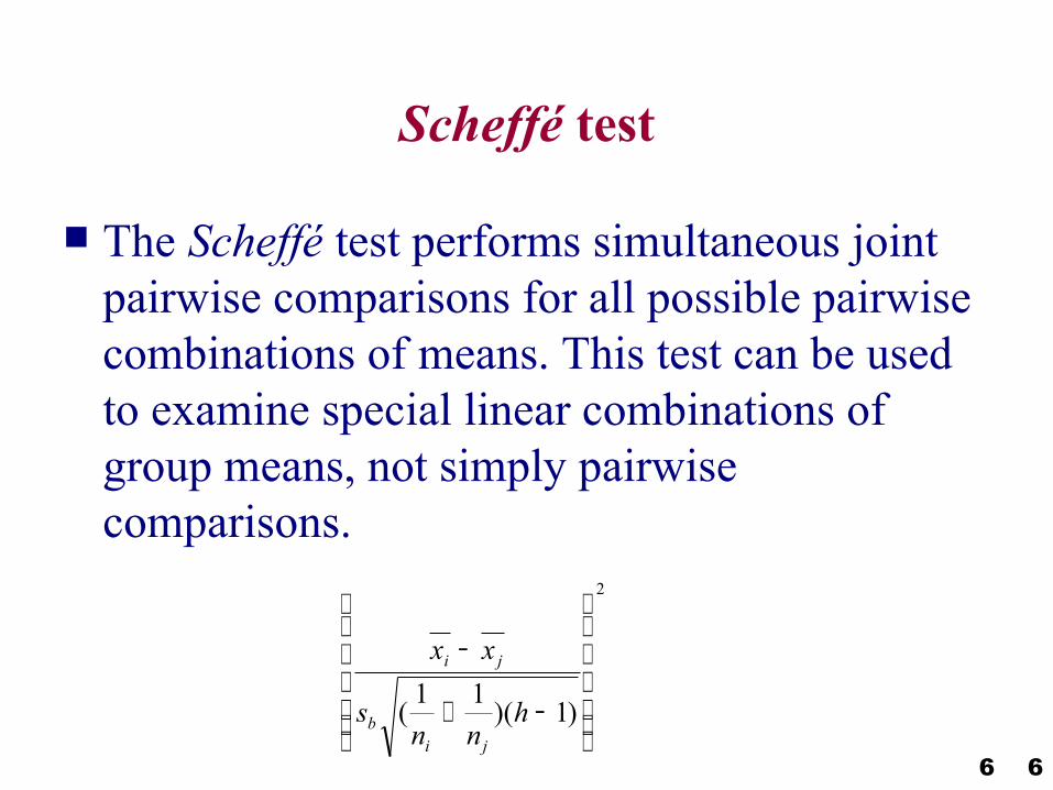
Scheffé test

The Scheffé test performs simultaneous joint pairwise comparisons for all possible pairwise combinations of means. This test can be used to examine special linear combinations of group means, not simply pairwise comparisons.

x x

sn n

h

i j

bi j

−

+ −

( )( )1 1 1

2


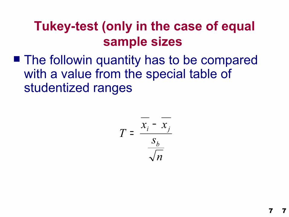
Tukey-test (only in the case of equal sample sizes

The followin quantity has to be compared with a value from the special table of studentized ranges

Tx x

sn

i j

b=

−


Dunnett test

Another multiple comparison method is the Dunnett test: a test comparing a given group (control) with the others.


Example Assume that we have recorded the

biomass of 3 bacteria in flasks of glucose broth, and we used 3 replicate flasks for each bacterium.

Replicate Bacterium A Bacterium B Bacterium C

1 12 20 40

2 15 19 35

3 9 23 42


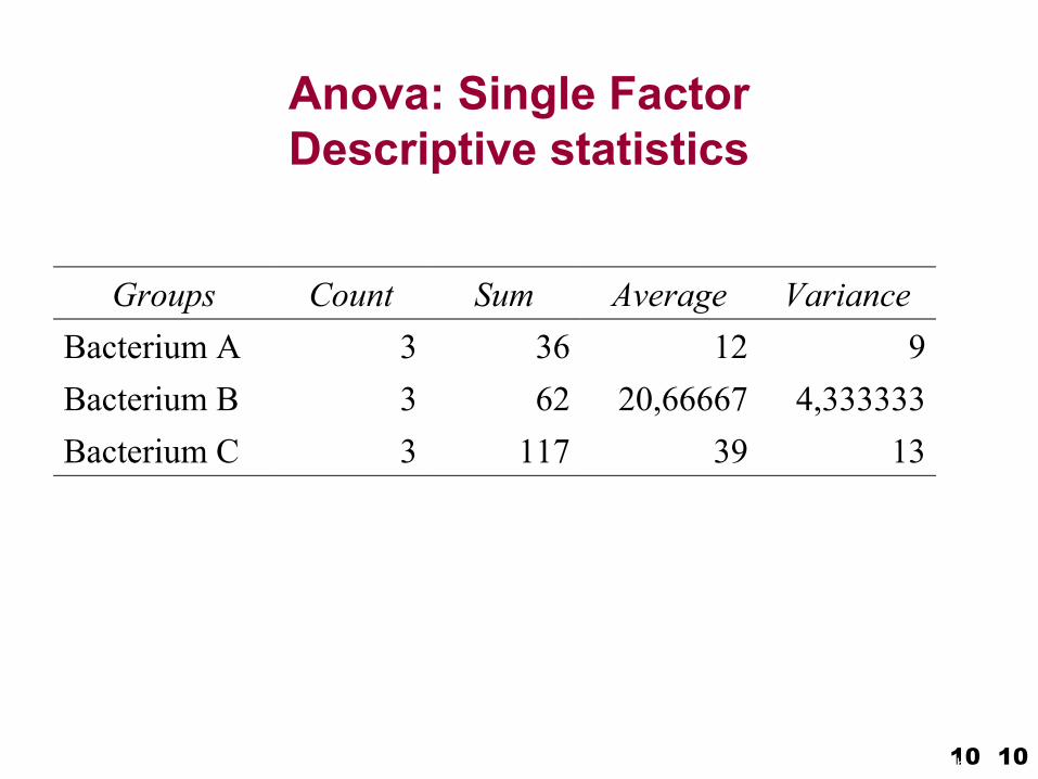
Anova: Single FactorDescriptive statistics

Groups Count Sum Average VarianceBacterium A 3 36 12 9Bacterium B 3 62 20,66667 4,333333Bacterium C 3 117 39 13


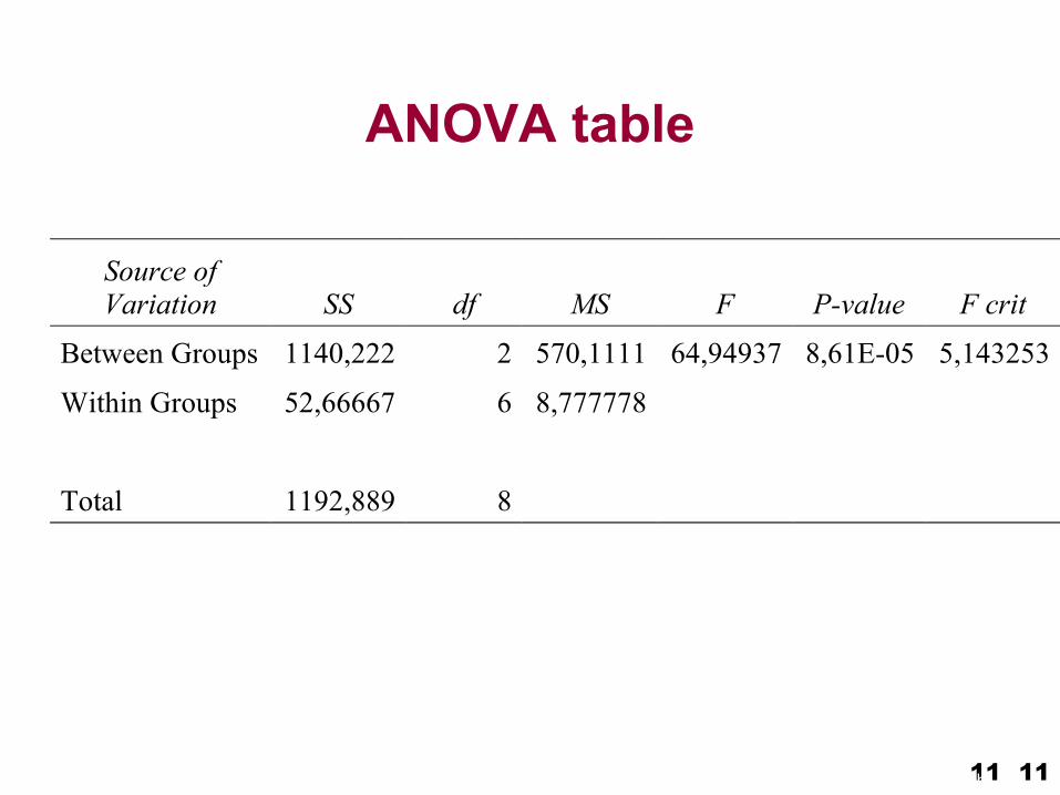
ANOVA table

Source of Variation SS df MS F P-value F crit

Between Groups 1140,222 2 570,1111 64,94937 8,61E-05 5,143253

Within Groups 52,66667 6 8,777778

Total 1192,889 8


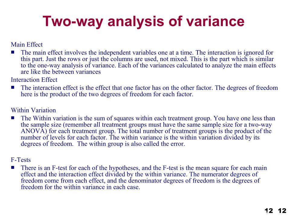
Two-way analysis of variance Main Effect The main effect involves the independent variables one at a time. The interaction is ignored for

this part. Just the rows or just the columns are used, not mixed. This is the part which is similar to the one-way analysis of variance. Each of the variances calculated to analyze the main effects are like the between variances

Interaction Effect The interaction effect is the effect that one factor has on the other factor. The degrees of freedom

here is the product of the two degrees of freedom for each factor.

Within Variation The Within variation is the sum of squares within each treatment group. You have one less than

the sample size (remember all treatment groups must have the same sample size for a two-way ANOVA) for each treatment group. The total number of treatment groups is the product of the number of levels for each factor. The within variance is the within variation divided by its degrees of freedom. The within group is also called the error.

F-Tests There is an F-test for each of the hypotheses, and the F-test is the mean square for each main

effect and the interaction effect divided by the within variance. The numerator degrees of freedom come from each effect, and the denominator degrees of freedom is the degrees of freedom for the within variance in each case.


Hypothesis There are three sets of hypothesis with the two-way ANOVA. The null hypotheses for each of the sets are given below. The population means of the first factor are equal. This is like the one-

way ANOVA for the row factor. The population means of the second factor are equal. This is like the

one-way ANOVA for the column factor. There is no interaction between the two factors. This is similar to

performing a test for independence with contingency tables.


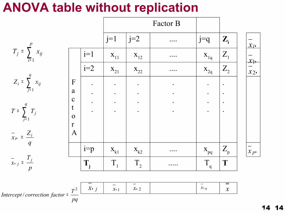
ANOVA table without replicationFactor B

j=1 j=2 .... j=q Zi

i=1 x11 x12 .... x1q Z1

i=2 x21 x22 .... x2q Z2

Factor A

.

.

.

.

.

.

.

.

.

.

.

.

.

.

.

.

.

.

.

.

.

.

.

.

i=p xk1 xk2 .... xpq Zp

Tj T1 T2 ..... Tq T

•ix

•1x•2x

•px

jx• 1•x 2•x qx • x

∑=

=p

iijj xT

1

∑=

=q

jiji xZ

1

∑=

=q

jjTT

1

qZx i

i =•

pT

x jj =•

pqTfactorcorrectionIntercept

2 / =


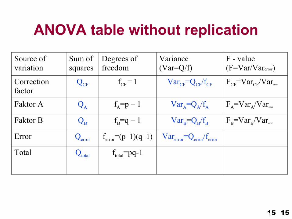
ANOVA table without replication

Source of variation

Sum of squares

Degrees of freedom

Variance(Var=Q/f)

F - value(F=Var/Varerror)

Correction factor

QCF fCF = 1 VarCF=QCF/fCF FCF=VarCF/Varerror

Faktor A QA fA=p – 1 VarA=QA/fA FA=VarA/Varerror

Faktor B QB fB=q – 1 VarB=QB/fB FB=VarB/Varerror

Error Qerror ferror=(p–1)(q–1) Varerror=Qerror/ferror

Total Qtotal ftotal=pq-1


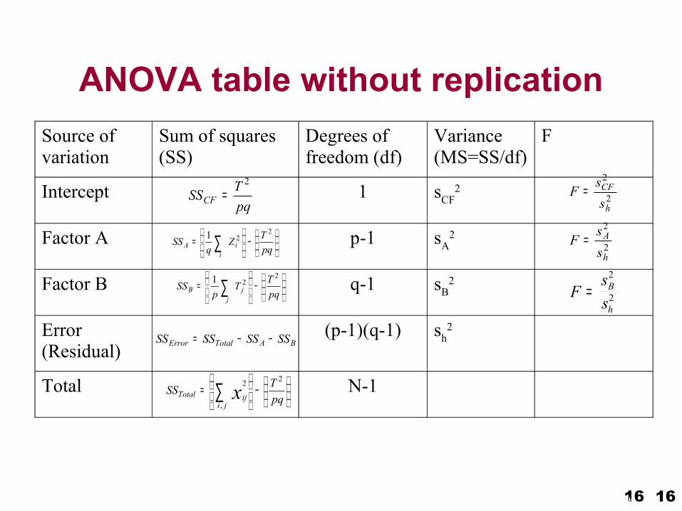
ANOVA table without replication

2

2

h

CF

ssF =

Fss

B

h=

2

2

Source of variation

Sum of squares (SS)

Degrees of freedom (df)

Variance (MS=SS/df)

F

Intercept 1 sCF2

Factor A p-1 sA2

Factor B q-1 sB2

Error (Residual)

(p-1)(q-1) sh2

Total N-1

pqTSSCF

2=

−

= ∑ pq

TZq

SSi

iA

221

2

2

h

A

ssF =

−

= ∑ pq

TTp

SSj

jB

221

−

= ∑ pq

TSSji

ijTotal x2

,

2

BATotalError SSSSSSSS −−=


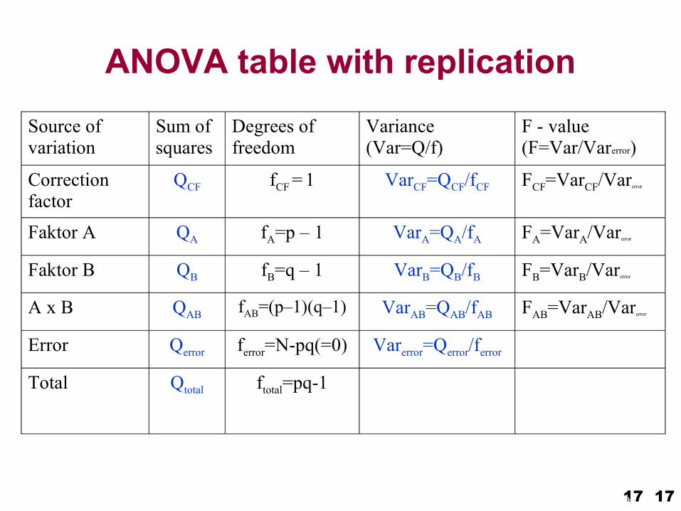
ANOVA table with replicationSource of variation

Sum of squares

Degrees of freedom

Variance(Var=Q/f)

F - value(F=Var/Varerror)

Correction factor

QCF fCF = 1 VarCF=QCF/fCF FCF=VarCF/Varerror

Faktor A QA fA=p – 1 VarA=QA/fA FA=VarA/Varerror

Faktor B QB fB=q – 1 VarB=QB/fB FB=VarB/Varerror

A x B QAB fAB=(p–1)(q–1) VarAB=QAB/fAB FAB=VarAB/Varerror

Error Qerror ferror=N-pq(=0) Varerror=Qerror/ferror

Total Qtotal ftotal=pq-1


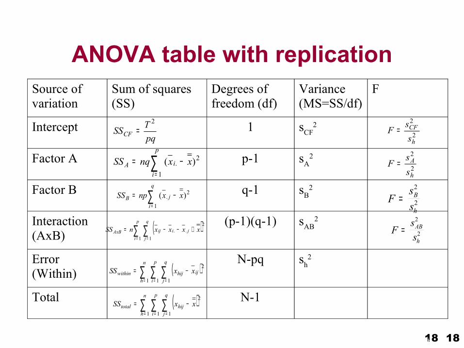
ANOVA table with replication

2

2

h

CF

ssF =

Fss

B

h=

2

2

FssAB

h=

2

2

Source of variation

Sum of squares (SS)

Degrees of freedom (df)

Variance (MS=SS/df)

F

Intercept 1 sCF2

Factor A p-1 sA2

Factor B q-1 sB2

Interaction (AxB)

(p-1)(q-1) sAB2

Error (Within)

N-pq sh2

Total N-1

2

2

h

A

ssF =

pqTSSCF

2=

∑=

−=p

iiA xxnqSS

1

2. )(

∑=

−=q

ijB xxnpSS

1

2. )(

( )∑ ∑ ∑= = =

−=n

h

p

i

q

jijhijwithin xxSS

1 1 1

2

( )∑ ∑= =

+−−=p

i

q

jjiijAxB xxxxnSS

1 1

2..

( )∑ ∑ ∑= = =

−=n

h

p

i

q

jhijtotal xxSS

1 1 1

2


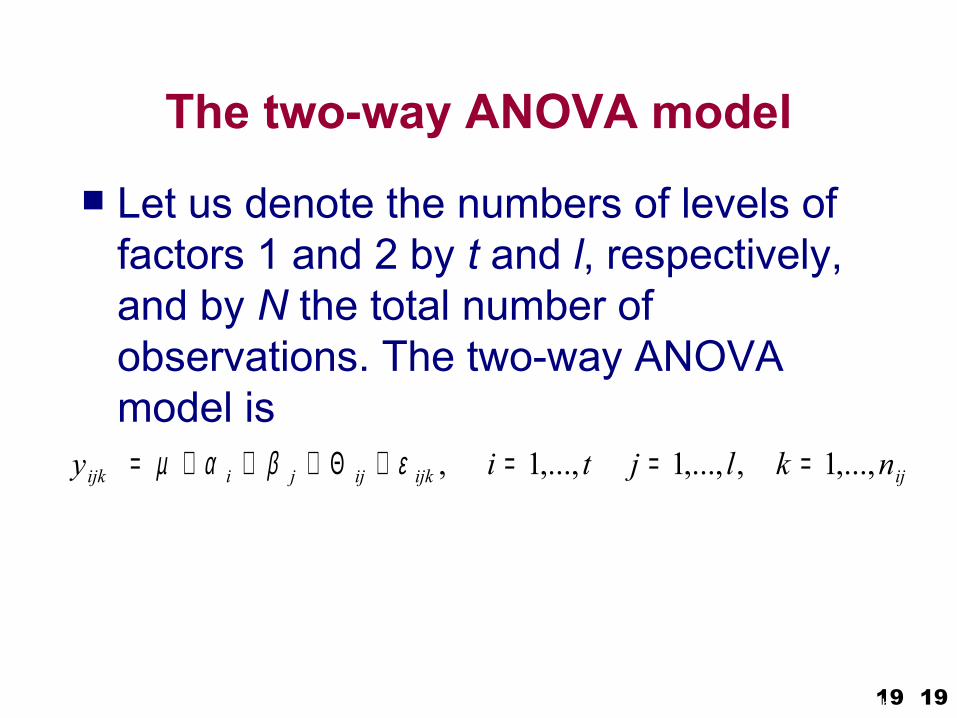
The two-way ANOVA model

Let us denote the numbers of levels of factors 1 and 2 by t and l, respectively, and by N the total number of observations. The two-way ANOVA model is

ijijkijjiijk nkljtiy ,...,1,,...,1,...,1, ===+Θ+++= εβαµ


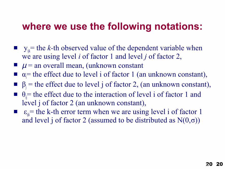
where we use the following notations:

yijk= the k-th observed value of the dependent variable when we are using level i of factor 1 and level j of factor 2,

µ = an overall mean, (unknown constant αi= the effect due to level i of factor 1 (an unknown constant), βj = the effect due to level j of factor 2, (an unknown constant), θij= the effect due to the interaction of level i of factor 1 and

level j of factor 2 (an unknown constant), εijk= the k-th error term when we are using level i of factor 1

and level j of factor 2 (assumed to be distributed as N(0,σ))


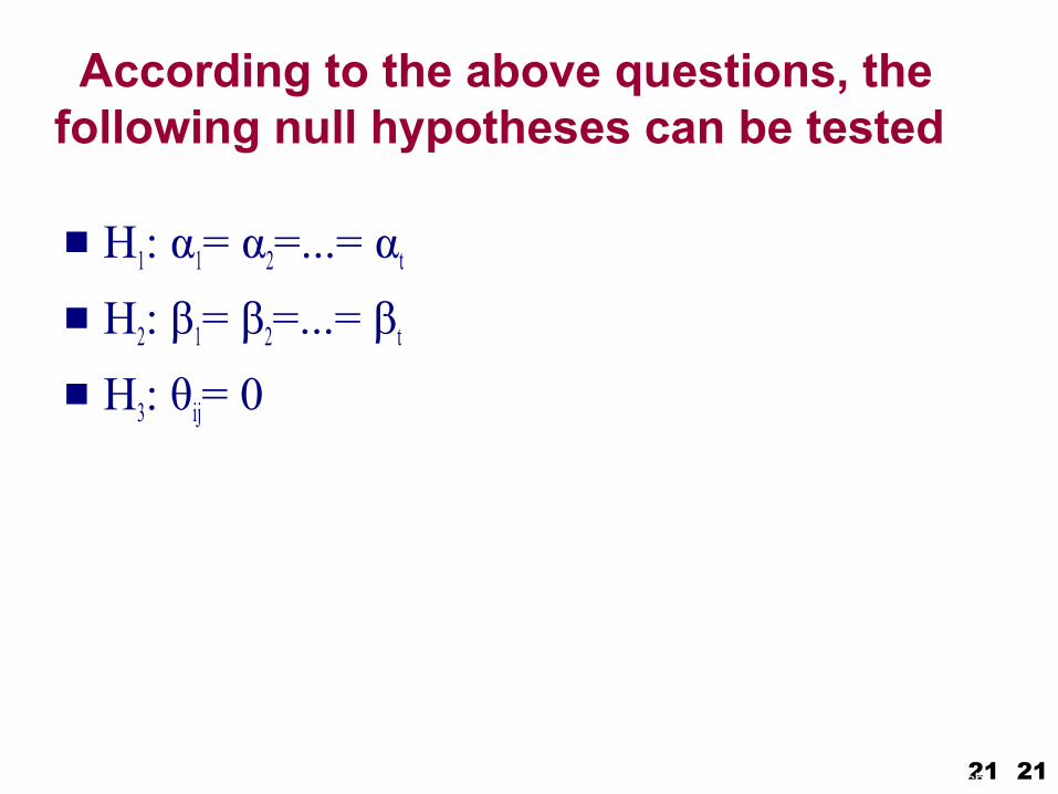
According to the above questions, the following null hypotheses can be tested

H1: α1= α2=...= αt

H2: β1= β2=...= βt

H3: θij= 0


Example:

Suppose that factor A has 3 levels (i=3) and factor B has 2 levels (j=2).

Them theoretically, we might have the following situations


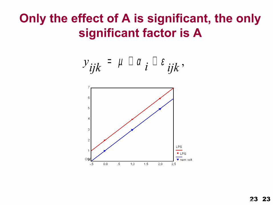
Only the effect of A is significant, the only significant factor is A

,ijkiijky εαµ ++=


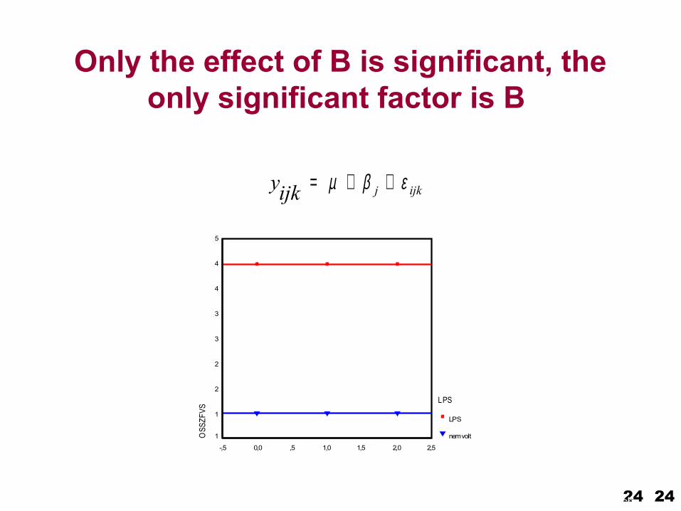
Only the effect of B is significant, the only significant factor is B

yijk j ijk= + +µ β ε

GD C L3

2,52,01,51,0,50,0-,5

OSS

ZFVS

5

4

4

3

3

2

2

1

1

LPS

LPS

nem volt


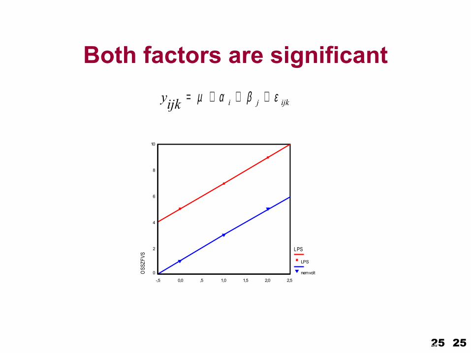
Both factors are significant

ijkjiijky εβαµ +++=

GD C L3

2,52,01,51,0,50,0-,5

OSS

ZFVS

10

8

6

4

2

0

LPS

LPS

nem volt


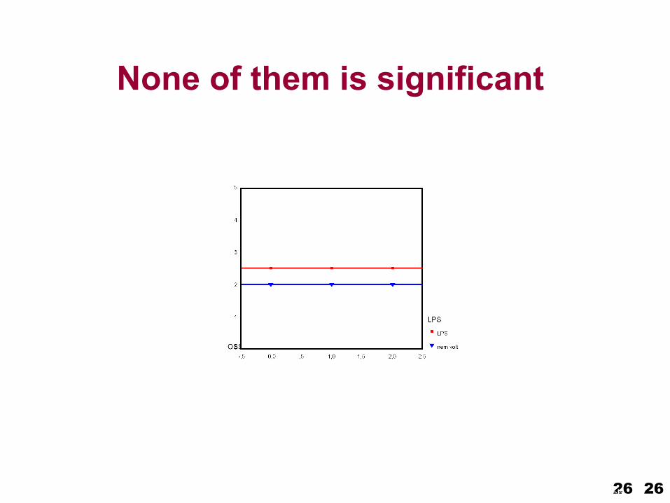
None of them is significant


Interaction

The differences in A depend on the level of factor B

GD C L3

2,52,01,51,0,50,0-,5

OSS

ZFVS

12

10

8

6

4

2

0

LPS

LPS

nem volt


Two-way ANOVA

In two-way ANOVA, the total sum of squares is decomposed into four terms, according to the effects in the model.

The results are generally written into an ANOVA table which contains rows for the effects of factors 1 and 2, the interaction and the error with (p-1), (q-1), (p-1)(q-1) and (N-pq) degrees of freedom, respectively


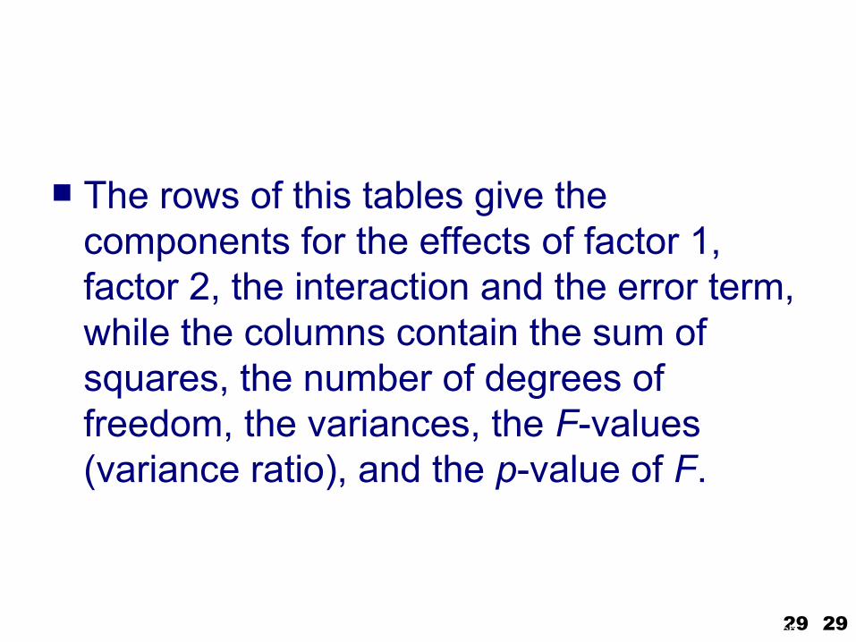
The rows of this tables give the components for the effects of factor 1, factor 2, the interaction and the error term, while the columns contain the sum of squares, the number of degrees of freedom, the variances, the F-values (variance ratio), and the p-value of F.


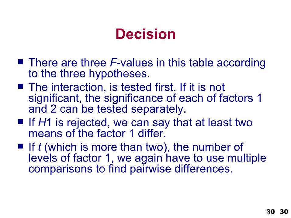
Decision

There are three F-values in this table according to the three hypotheses.

The interaction, is tested first. If it is not significant, the significance of each of factors 1 and 2 can be tested separately.

If H1 is rejected, we can say that at least two means of the factor 1 differ.

If t (which is more than two), the number of levels of factor 1, we again have to use multiple comparisons to find pairwise differences.


Decision

If the interaction is significant, then the relationship between the means of factor 1 depends on the level of factor 2. Multiple comparisons can be performed for each combination of one factor with a given level of the other factor.

There are special methods against the increase of Type I error, and the use of t-tests independently is an incorrect solution


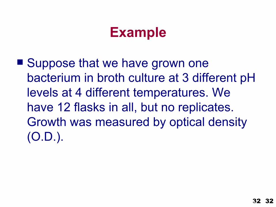
Example

Suppose that we have grown one bacterium in broth culture at 3 different pH levels at 4 different temperatures. We have 12 flasks in all, but no replicates. Growth was measured by optical density (O.D.).


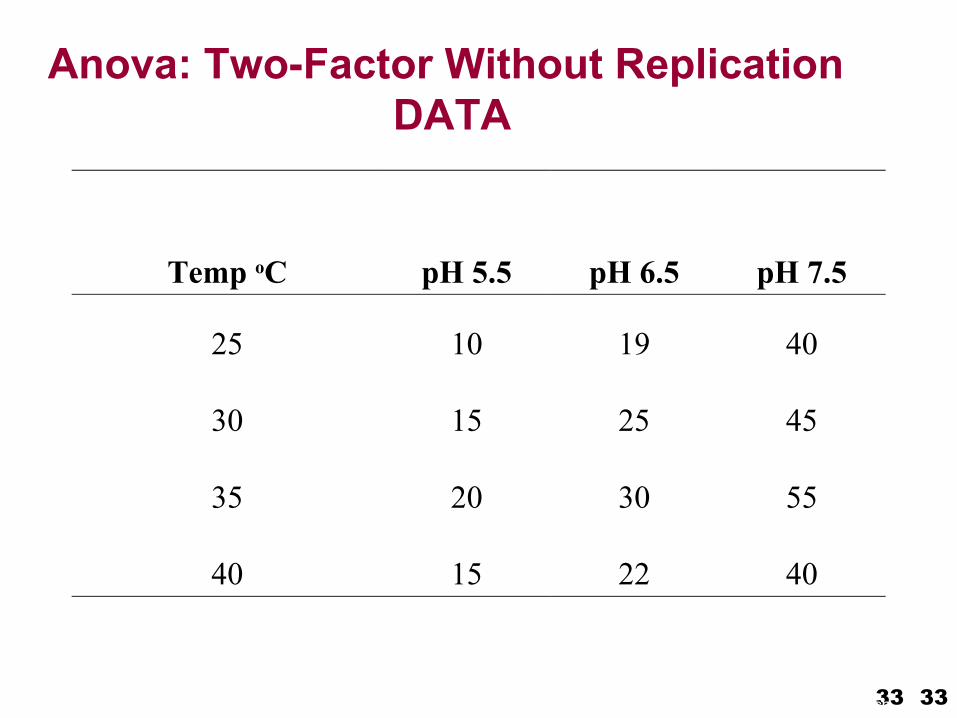
Anova: Two-Factor Without Replication DATA

Temp oC pH 5.5 pH 6.5 pH 7.5

25 10 19 40

30 15 25 45

35 20 30 55

40 15 22 40


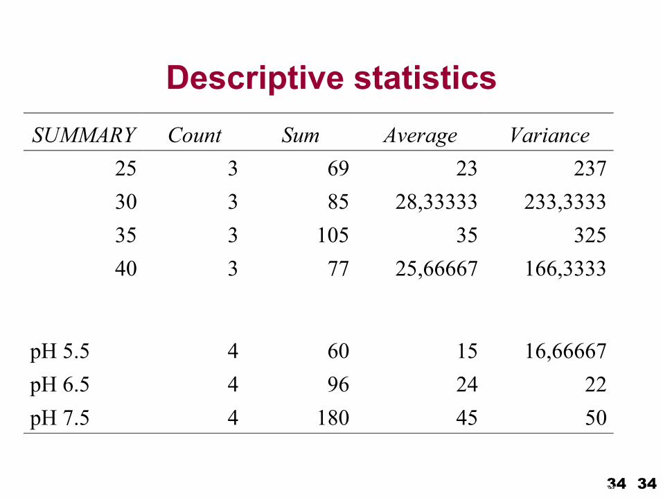
Descriptive statisticsSUMMARY Count Sum Average Variance

25 3 69 23 23730 3 85 28,33333 233,333335 3 105 35 32540 3 77 25,66667 166,3333

pH 5.5 4 60 15 16,66667pH 6.5 4 96 24 22pH 7.5 4 180 45 50


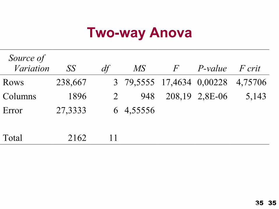
Two-way AnovaSource of

Variation SS df MS F P-value F critRows 238,667 3 79,5555 17,4634 0,00228 4,75706Columns 1896 2 948 208,19 2,8E-06 5,143Error 27,3333 6 4,55556

Total 2162 11


Of interest, another piece of information is revealed by this analysis - the effects of temperature do not interact with effects of pH. In other words, a change of temperature does not change the response to pH, and vice-versa.We can deduce this because the residual (error) mean square (MS) is small compared with the mean squares for temperature (columns) or pH (rows). [A low residual mean square tells us that most variation in the data is accounted for by the separate effects of temperature and pH].


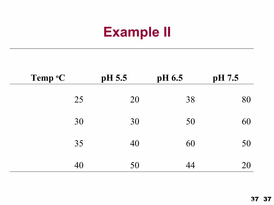
Example II

Temp oC pH 5.5 pH 6.5 pH 7.5

25 20 38 80

30 30 50 60

35 40 60 50

40 50 44 20


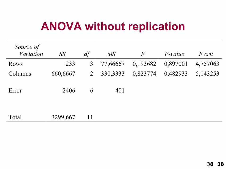
ANOVA without replicationSource of

Variation SS df MS F P-value F critRows 233 3 77,66667 0,193682 0,897001 4,757063Columns 660,6667 2 330,3333 0,823774 0,482933 5,143253

Error 2406 6 401

Total 3299,667 11


ANOVA with replication

The data of serum IGG level were measured in triplicate of three patients.

Is there any difference in individual mean IGG level values using diferent method of measurement?


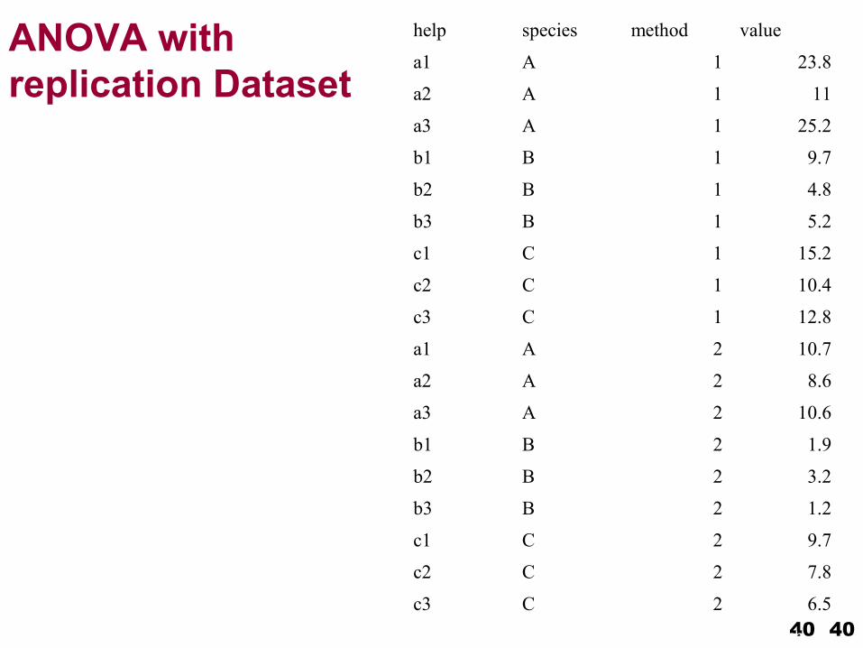
ANOVA with replication Dataset

help species method value

a1 A 1 23.8

a2 A 1 11

a3 A 1 25.2

b1 B 1 9.7

b2 B 1 4.8

b3 B 1 5.2

c1 C 1 15.2

c2 C 1 10.4

c3 C 1 12.8

a1 A 2 10.7

a2 A 2 8.6

a3 A 2 10.6

b1 B 2 1.9

b2 B 2 3.2

b3 B 2 1.2

c1 C 2 9.7

c2 C 2 7.8

c3 C 2 6.540HUSRB/0901/221/088 „Teaching Mathematics and Statistics in Sciences: Modeling and Computer-aided Approach 40

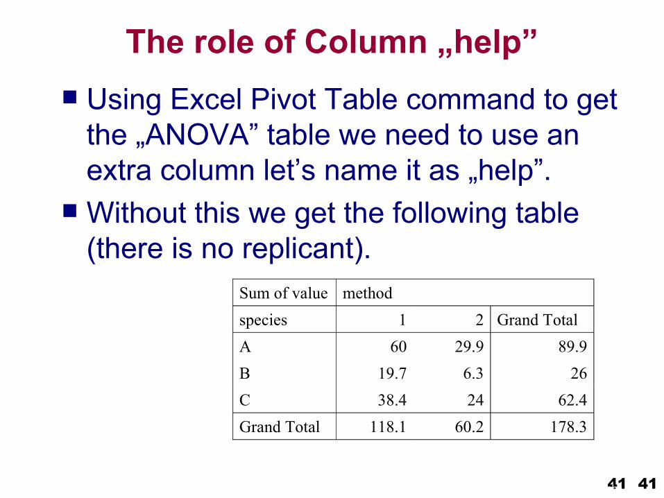
The role of Column „help” Using Excel Pivot Table command to get

the „ANOVA” table we need to use an extra column let’s name it as „help”.

Without this we get the following table (there is no replicant).

Sum of value method species 1 2 Grand TotalA 60 29.9 89.9B 19.7 6.3 26C 38.4 24 62.4Grand Total 118.1 60.2 178.3


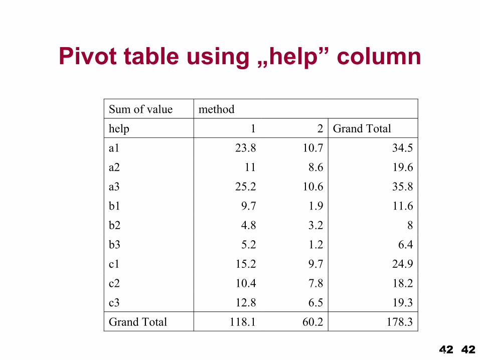
Pivot table using „help” column

Sum of value method help 1 2 Grand Totala1 23.8 10.7 34.5a2 11 8.6 19.6a3 25.2 10.6 35.8b1 9.7 1.9 11.6b2 4.8 3.2 8b3 5.2 1.2 6.4c1 15.2 9.7 24.9c2 10.4 7.8 18.2c3 12.8 6.5 19.3Grand Total 118.1 60.2 178.3


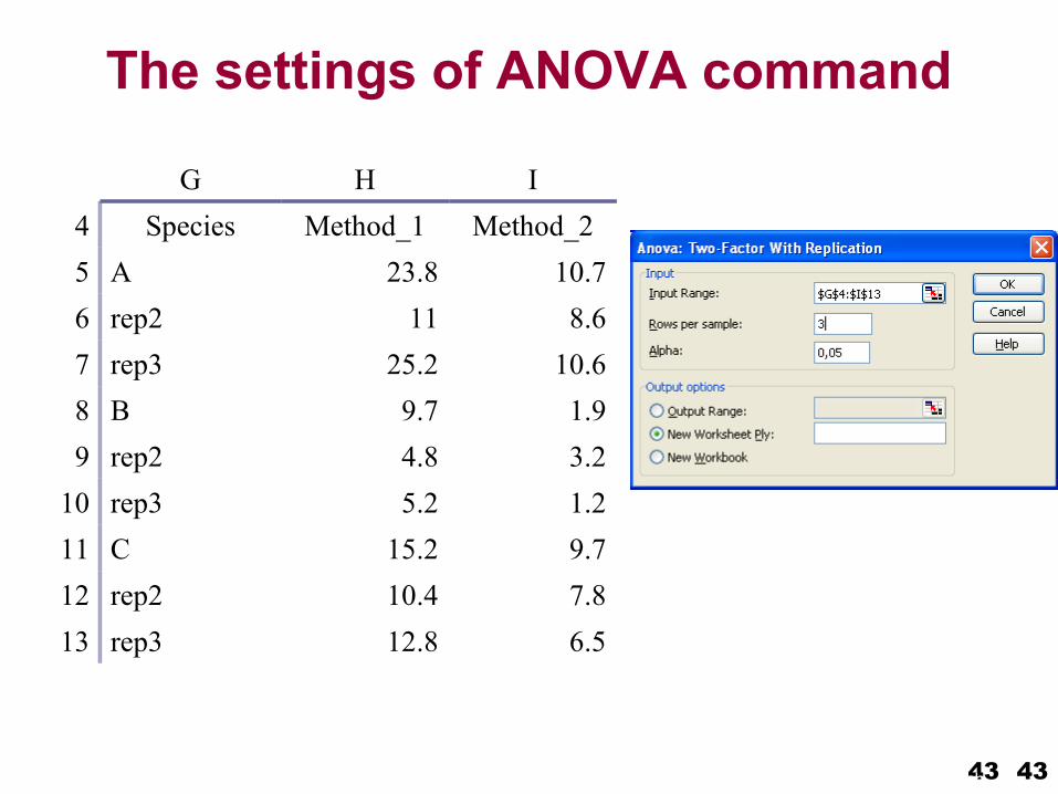
The settings of ANOVA command

G H I4 Species Method_1 Method_25 A 23.8 10.76 rep2 11 8.67 rep3 25.2 10.68 B 9.7 1.99 rep2 4.8 3.2

10 rep3 5.2 1.211 C 15.2 9.712 rep2 10.4 7.813 rep3 12.8 6.5


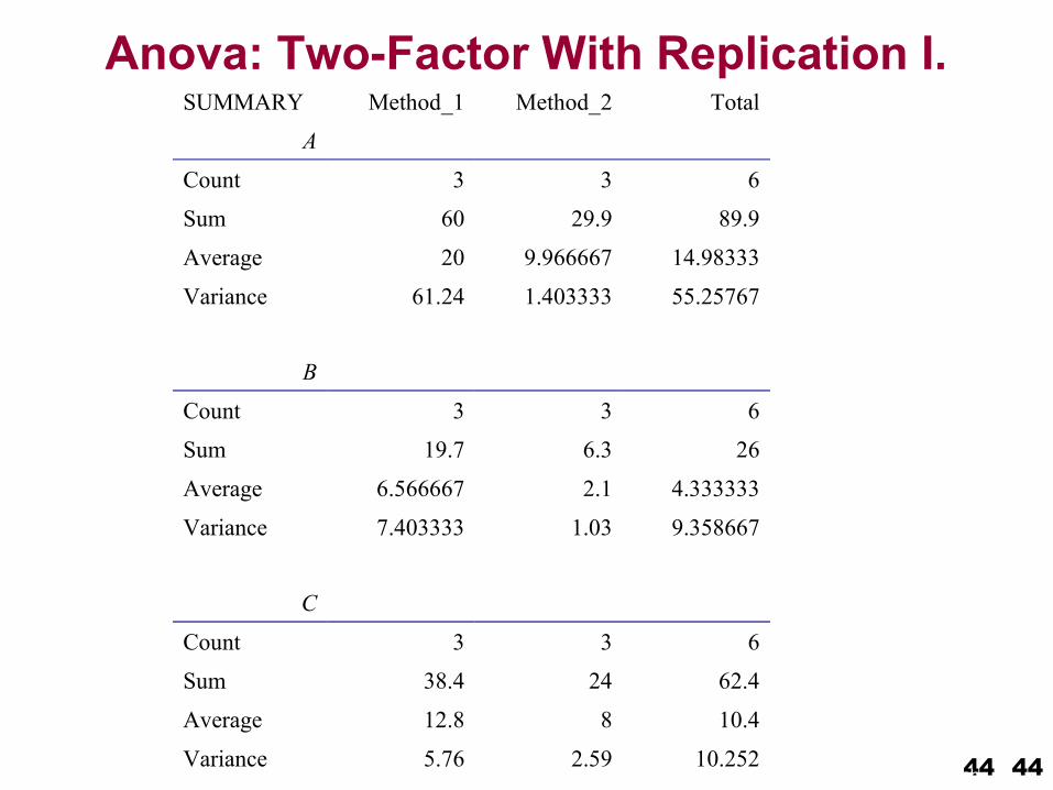
Anova: Two-Factor With Replication I.SUMMARY Method_1 Method_2 Total

A

Count 3 3 6

Sum 60 29.9 89.9

Average 20 9.966667 14.98333

Variance 61.24 1.403333 55.25767

B

Count 3 3 6

Sum 19.7 6.3 26

Average 6.566667 2.1 4.333333

Variance 7.403333 1.03 9.358667

C

Count 3 3 6

Sum 38.4 24 62.4

Average 12.8 8 10.4

Variance 5.76 2.59 10.252 44HUSRB/0901/221/088 „Teaching Mathematics and Statistics in Sciences: Modeling and Computer-aided Approach 44

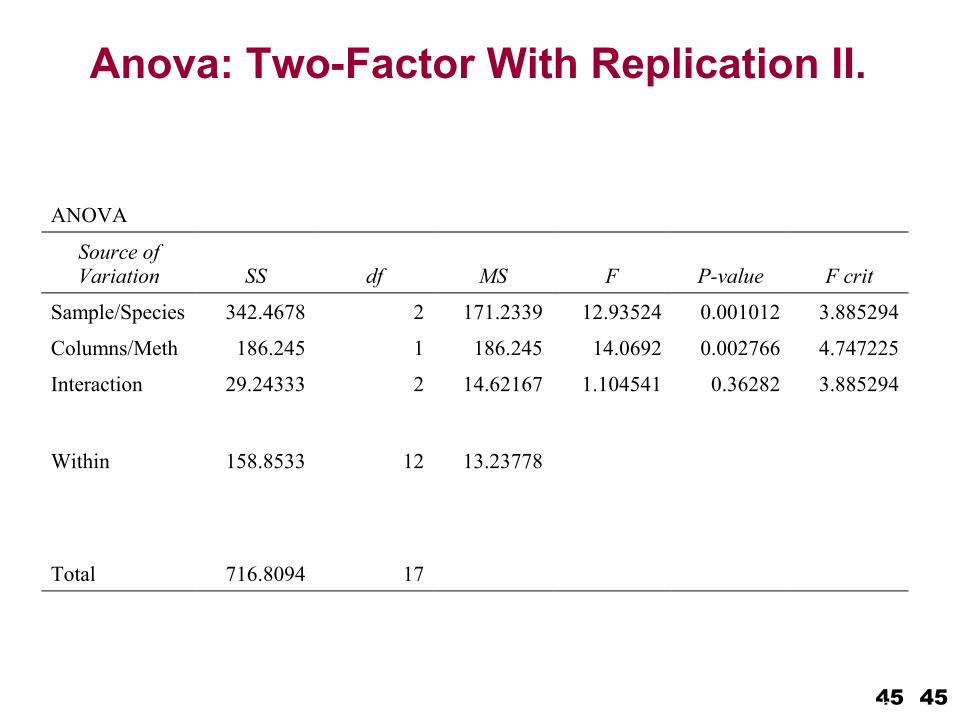
Anova: Two-Factor With Replication II.

ANOVA

Source of Variation SS df MS F P-value F crit

Sample/Species 342.4678 2 171.2339 12.93524 0.001012 3.885294

Columns/Meth 186.245 1 186.245 14.0692 0.002766 4.747225

Interaction 29.24333 2 14.62167 1.104541 0.36282 3.885294

Within 158.8533 12 13.23778

Total 716.8094 17


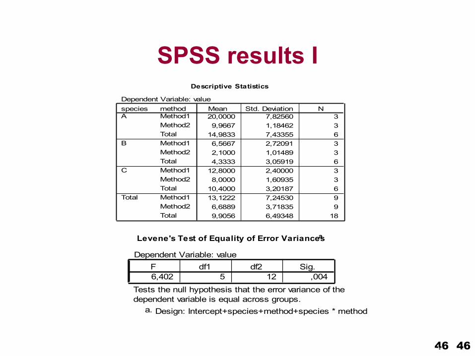
SPSS results IDescriptive Statistics

Dependent Variable: value

20,0000 7,82560 39,9667 1,18462 3

14,9833 7,43355 66,5667 2,72091 32,1000 1,01489 34,3333 3,05919 6

12,8000 2,40000 38,0000 1,60935 3

10,4000 3,20187 613,1222 7,24530 96,6889 3,71835 99,9056 6,49348 18

methodMethod1Method2TotalMethod1Method2TotalMethod1Method2TotalMethod1Method2Total

speciesA

B

C

Total

Mean Std. Deviation N

Levene's Test of Equality of Error Variancesa


6,402 5 12 ,004F df1 df2 Sig.

Tests the null hypothesis that the error variance of thedependent variable is equal across groups.

Design: Intercept+species+method+species * methoda.


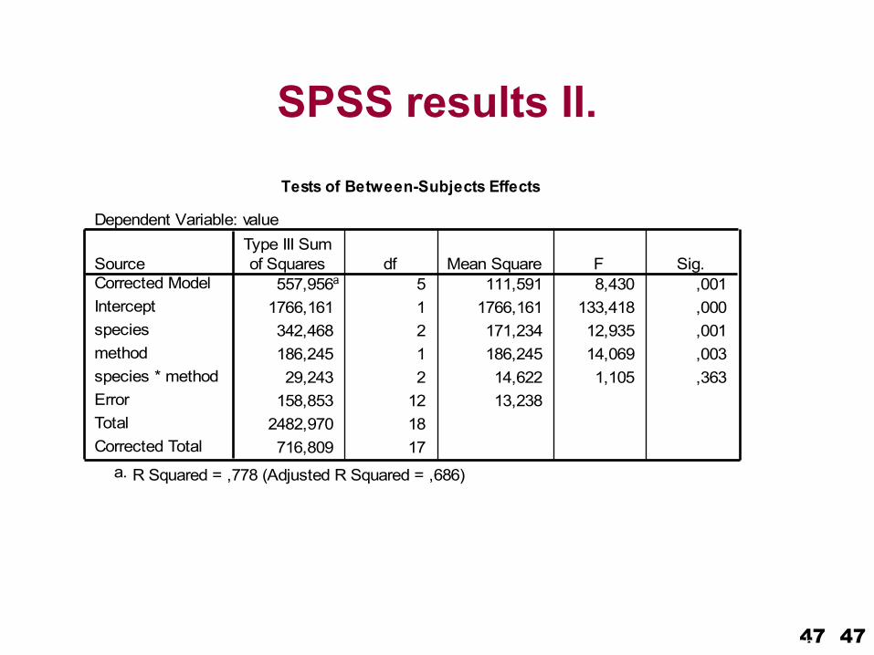
SPSS results II.Tests of Between-Subjects Effects


557,956a 5 111,591 8,430 ,0011766,161 1 1766,161 133,418 ,000342,468 2 171,234 12,935 ,001186,245 1 186,245 14,069 ,00329,243 2 14,622 1,105 ,363

158,853 12 13,2382482,970 18716,809 17

SourceCorrected ModelInterceptspeciesmethodspecies * methodErrorTotalCorrected Total

Type III Sumof Squares df Mean Square F Sig.

R Squared = ,778 (Adjusted R Squared = ,686)a.


Post-Hoc test

Multiple Comparisons

Dependent Variable: valueLSD

10,6500* 2,10062 ,000 6,0731 15,22694,5833* 2,10062 ,050 ,0065 9,1602

-10,6500* 2,10062 ,000 -15,2269 -6,0731-6,0667* 2,10062 ,014 -10,6435 -1,4898-4,5833* 2,10062 ,050 -9,1602 -,00656,0667* 2,10062 ,014 1,4898 10,6435

(J) speciesBCACAB

(I) speciesA

B

C

MeanDifference

(I-J) Std. Error Sig. Lower Bound Upper Bound95% Confidence Interval

Based on observed means.The mean difference is significant at the ,05 level.*.


Documents

Analysis of variance filevariance in two distinct ways: ... The results of computations of ANOVA methods are usually tabulated. The rows of such tables give the source of the variance;