ANALYSIS OF LAMINATED CURVED BEAM WITH AND WITHOUT …

i

ANALYSIS OF LAMINATED CURVED BEAM WITH AND WITHOUT

DEFECTS AND IMPERFECTIONS

by

WEI-TSEN LU

DISSERTATION

Submitted in partial fulfilment of the requirements

for the degree of Doctor of Philosophy in Aerospace Engineering at

The University of Texas at Arlington

August, 2019

Supervising Committee:

Dr. Endel V. Iarve, Supervising Professor

Dr. Erian Armanios

Dr. Seiichi Nomura

Dr. Andrey Beyle

Dr. Ashfaq Adnan

Dr. Shih-Ho Chao

ii

Copyright @ by Wei-Tsen Lu 2019

All Right Reserved

iii

Abstract

ANALYSIS OF LAMINATED CURVED BEAM WITH AND WITHOUT DEFECTS

AND IMPERFECTIONS

Wei-Tsen Lu, PhD

The University of Texas at Arlington, 2019

Supervising Professor: Endel V. Iarve

Several studies have focused on the modeling and response characterization of

composite structural members, with particular emphasis on composite curved

beams. The class of curved beam is explored to determine mechanical response in

primary aerospace structural applications. The present work focuses on developing

analytical closed-form solutions for investigating composite curved beams with and

without fiber waviness and delamination. The present work can efficiently

characterize the structural behavior of composite curved beams under bending.

This work shows the development of a novel mathematical approach to

predict structural performance by investigating axial stiffness, bending stiffness

with consideration of shear deformation in composite curved beam. A modified

Classical Lamination Theory (CLT) is proposed by considering cross-section effect

of a beam. Finite Element (FE) analysis is employed to compare against the

analytical results. Parametric study is conducted to investigate effects of radius of

composite curved beam versus axial and bending stiffness. Ply stress variations are

also studied for a composite curved beam under bending. The stress results obtained

from numerical analysis show excellent agreement in comparison with present

approach.

iv

The present work also studied fiber waviness effect in composite curved

beam. Fiber waviness has an adverse influence on the mechanical properties. The

tensile, compressive strength, and fatigue life degrade significantly due to fiber

waviness. The proposed method takes into account the degraded stiffness properties

by considering various amplitude-length ratio of fiber waviness presented in curved

beam. It can be concluded that for a composite curved beam with fiber waviness,

the effect of stiffness reduction significantly increases if the amplitude-length ratio

is between 0.6 and 1.0. Moreover, the present work provides an analytical solution

to predict the interlaminar radial stress 𝜎𝑟 if fiber waviness is present. The

analytical results show excellent agreement with results obtained from numerical

analysis.

Delamination is considered as one of the dominant failure factor in

composite and leads to substantial stiffness loses. The present work provides an

analytical method for calculation of the strain energy release rate (ERR) of a

delamination in a composite curved beam. In the present approach, we allow for a

delamination which is not symmetric with respect to the middle span of the

composite curved beam and can be located at any arbitrary interface.

v

ACKNOWLEDGEMENTS

This work could not have been done without supports and encouragement

of numerous people to whom I would like to express my appreciation.

First, I would like to express my profoundly gratitude to my advising

Professor Dr. Endel V. Iarve for devoting his invaluable time to guide me with

constant encouragement. I am indebted for plentiful enlightening discussions and

inspiring critiques, which makes me become a better researcher. I am also grateful

to my distinguished professor and mentor, Dr. Erian Armanios, who always gives

me great support and encouragement in every aspect. The knowledge I could

always count on him and his support that made UT-Arlington feel like home. I am

deeply appreciated his unconditional help and guide. I would also like to express

my sincere appreciations to my committee members Dr. Seiichi Nomura and Dr.

Ashfaq Adnan, for their helps and assistances not only in Ph.D. but the master

program as well. In addition, the time and valuable feedback from Dr. Andrey

Beyle and Dr. Shih-Ho Chao so generously provided has been instrumental in the

successful completion of my research. I want to express my sincere appreciation to

Dr. Stefan Dancila, who gave me unconditional support when I need help.

I would like to thank the entire faculty and staff of Mechanical and

Aerospace Engineering Department for their helps. Special thanks go to Lanie,

Flora, Ayesha, Kathy, Janet, Catherine, Wendy and Danette.

I would like to express my endless love to my parents and my best brother.

This honor goes to my entire family.

I would like to thank my friends, Ray, Hari, Scott, and Kevin for their

assistance in the dissertation and dedicated technical support.

vi

I would like to express my special acknowledgement to my wife, Jean.

Without her understanding and supports, this dissertation would not have been

completed.

Finally, I want to express my deepest acknowledge to my mentor, Dr. Wen

S. Chan. Without him, I couldn’t pursue PhD at the beginning. I learned many

things from him. He corrected my weakness and accompanied me, made my life

colorful day after day. I will always consider him as my “Academic Father”. He

was a memorable person and everybody will miss him. How humble he was, how

accomplished he was. I will make you proud because I am proud to say “It’s my

honor for having you to be my teacher”. Thank you, thank you and thank you.

vii

Table of Contents

Abstract ........................................................................................................................................... iii

ACKNOWLEDGEMENTS ............................................................................................................. v

List of Figures ................................................................................................................................. xi

List of Table ................................................................................................................................. xvii

.......................................................................................................................................... 1

LITERATURE SURVEY ................................................................................................................ 1

1-1 Composite Curved Beam ......................................................................... 1

1-2 Fiber Waviness ......................................................................................... 2

1-3 Composite Curved Beam with Delamination........................................... 5

.......................................................................................................................................... 7

RESEARCH OBJECTIVES ............................................................................................................ 7

.......................................................................................................................................... 9

OVERVIEW OF CLASSICAL LAMINATION THEORY ............................................................ 9

3-1 Lamina Stage ............................................................................................ 9

3-2 Stress Transformation ............................................................................ 10

3-3 Laminate Stage (Classical Lamination Theory) ..................................... 12

........................................................................................................................................ 17

STIFFNESS AND STRESS INVESTIGATION OF COMPOSITE CURVED BEAM ................ 17

4-1 Stiffness Model Formulation for Composite Curved Beam .................. 17

4-2 Modified Stiffness Approach for Composite Beam ............................... 20

4.2.1. Wide Beam (WB) ........................................................................... 20

4.2.2. Narrow Beam (NB) ......................................................................... 22

4-3 Ply-Stress Investigation .......................................................................... 23

viii

4-4 Effective Stiffness Results and Discussion ............................................ 30

........................................................................................................................................ 34

COMPOSITE CURVED BEAM WITH FIBER WAVINESS ...................................................... 34

5-1 Effective Stiffness Properties for Straight In-Plane Lamina with Fiber

Waviness ........................................................................................................... 34

5-2 Effective Stiffness Properties for Straight Out-of-Plane Lamina with Fiber

Waviness ........................................................................................................... 36

5-3 Effective Stiffness Properties of Composite Straight Laminate with In-

Plane and Out-of-Plane Fiber Waviness ........................................................... 38

5-4 Incremental Loading Scheme ................................................................. 40

5-5 Effective Stiffness Properties for Composite Curved Beam with In-Plane

and Out-of-Plane Fiber Waviness ..................................................................... 42

5-6 Maximum Radial Stress Prediction ........................................................ 44

5-7 Finite Element Analysis ......................................................................... 45

5.7.1. In-Plane Straight Lamina with Fiber Waviness .............................. 45

5.7.2. Out-of-Plane Curved Laminate with Fiber Waviness ..................... 48

5-8 Results and Discussion ........................................................................... 51

5.8.1. In-Plane Fiber Waviness for 0° Lamina ......................................... 51

5.8.2. In-Plane Fiber Waviness for 𝜃° Lamina ......................................... 54

5.8.3. Effects of Fiber Waviness Parameter 𝑅 .......................................... 62

5.8.4. Incremental Load Study of In-Plane Fiber Waviness of 0° Lamina 63

5.8.5. Out-of-Plane Fiver Waviness for 𝜃° Laminate ............................... 69

5.8.6. In-Plane Fiber Waviness of 0° Curved Lamina .............................. 71

ix

5.8.7. Out-of-Plane Fiber Waviness of 0° Curved Laminate .................... 72

5.8.8. Maximum Radial Stress Prediction for Composite Curved Beam with

Out-of-Plane Fiber Waviness under Bending ............................................... 74

5-9 Conclusion .............................................................................................. 76

........................................................................................................................................ 77

COMPOSITE CURVED BEAM WITH DELAMINATION ........................................................ 77

6-1 Symmetrical Model Formulation ........................................................... 77

6-2 Unsymmetrical Model Formulation ....................................................... 82

6-3 Finite Element Analysis ......................................................................... 85

6.3.1. Model Formulation ......................................................................... 85

6-4 Results and Discussion ........................................................................... 88

6.4.1. Radial Effect ................................................................................... 88

6.4.2. Length Effect .................................................................................. 92

6.4.3. Hoop Effect ..................................................................................... 96

6-5 Conclusion .............................................................................................. 98

...................................................................................................................................... 100

TORSIONAL AND WARPING STIFFNESS OF COMPOSITE Z-STIFFENERS .................... 100

7-1 Introduction .......................................................................................... 100

7-2 Constitutive Equation of Isotropic Z-Stiffener..................................... 102

7.2.1. Torsional Stiffness of Isotropic Z-Stiffener .................................. 102

7.2.2. Warping Stiffness of Isotropic Beam ............................................ 104

7.2.3. Warping Stiffness of Isotropic Z-Stiffener ................................... 107

7-3 Constitutive Equation of Composite Z-Stiffener ................................. 111

x

7-3.1 Constitutive Equation of Laminated Composite Beam under Torsion

111

7-3.2 Shear Center .................................................................................. 113

7-3.3 Torsional Stiffness of Composite Z-Stiffener ............................... 118

7-3.4 Warping Stiffness of Composite Z-Stiffener ................................ 121

7-4 Finite Element Analysis for Composite Z-Stiffener ............................ 122

7-4.1 Model Definition and Boundary Condition .................................. 123

7-4.2 Torsional and Warping Stiffness in Finite Element Analysis ....... 125

7-5 Results and Discussion ......................................................................... 125

7-5.1 Isotropic Validation ...................................................................... 125

7-5.2 Composite Validation ................................................................... 130

7-5.3 Comparison between Narrow and Wide Beam Assumption for

Composite Z-Stiffener ................................................................................ 138

7-6 Conclusion for Composite Z-Stiffener ................................................. 140

...................................................................................................................................... 141

CONCLUSION AND FURTURE WORK .................................................................................. 141

Appendix A .................................................................................................................................. 145

Appendix B .................................................................................................................................. 149

Appendix C .................................................................................................................................. 153

REFERENCE ............................................................................................................................... 160

xi

List of Figures

Figure 3-1 x-y coordinate system for a 0° lamina and 1-2 coordinate system for a

θ° lamina. ...................................................................................................... 11

Figure 4-1 The configuration of curved beam. ..................................................... 18

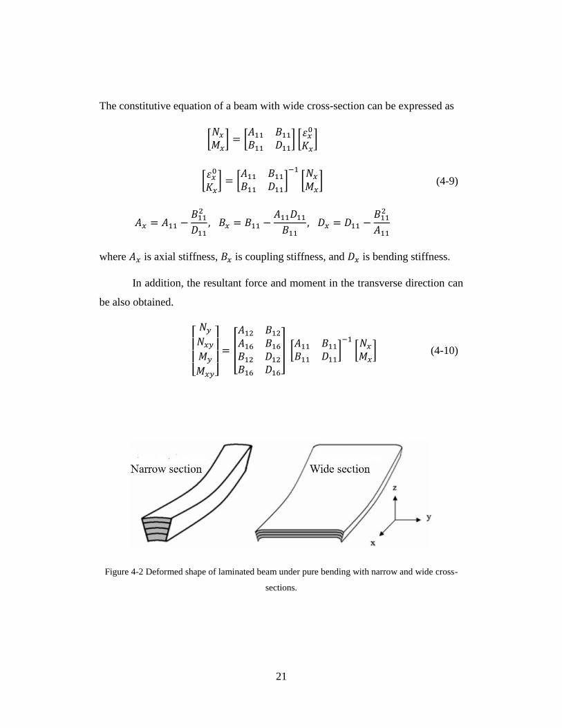
Figure 4-2 Deformed shape of laminated beam under pure bending with narrow and

wide cross-sections. ...................................................................................... 21

Figure 4-3 Geometry of curved beam under bending moment 𝑀, shear force 𝑄, and

axial force 𝑁. ................................................................................................. 24

Figure 4-4 Definition of ply radius [65]. .............................................................. 27

Figure 4-5 Stress distribution for a composite curved beam under bending (a)

tangential stress 𝜎𝜃 (b) radial stress 𝜎𝑟 ........................................................ 28

Figure 4-6 𝜎𝑟 distribution for a composite curved beam under bending (Eqs. 4-24).

....................................................................................................................... 29

Figure 4-7 Difference between general (Eqs. 4-7), wide (Eqs. 4-9) and narrow (Eqs.

4-15) section for a beam with initial curvature. ............................................ 31

Figure 4-8 𝜎𝜃 comparison using stiffness under general, wide, and narrow beam

assumptions. .................................................................................................. 33

Figure 5-1 (a) 2-D in-plane fiber waviness geometry. (b) 3-D in-plane fiber

waviness geometry. ....................................................................................... 35

Figure 5-2 D out-of-plane fiber waviness geometry. ............................................ 36

Figure 5-3 Out-of-plane fiber waviness in laminate stage with in-plane fiber

orientation. .................................................................................................... 39

xii

Figure 5-4 Flow chart for finding updated fiber waviness amplitude after every

incremental strain. ......................................................................................... 41

Figure 5-5 (a) In-plane fiber waviness in a curved lamina. (b) Out-of-plane fiber

waviness in a curved beam. .......................................................................... 43

Figure 5-6 Geometry of in-plane fiber waviness. ................................................. 46

Figure 5-7(a) Displacement along 1-direction. (b) Displacement along 2-direction.

....................................................................................................................... 47

Figure 5-8 Shear distribution for an in-plane lamina with fiber waviness under

tension. .......................................................................................................... 48

Figure 5-9 (a) Perfect bonded layers (b) Boundary conditions and applied moment.

....................................................................................................................... 49

Figure 5-10 Finite Element analysis 𝜎1 and 𝜎2 results using isotropic material

properties (𝐸 = 30 𝑀𝑃𝑎 and 𝑣 = 0.3). ........................................................ 49

Figure 5-11 Comparison between Young’s moduli and waviness parameter 𝑅. .. 52

Figure 5-12 Shear moduli vs fiber waviness parameter 𝑅. ................................... 52

Figure 5-13 Poisson’s ratios vs fiber waviness parameter 𝑅. ............................... 53

Figure 5-14 CTEs vs fiber waviness parameter 𝑅. ............................................... 53

Figure 5-15 𝐸x vs waviness ratio, R with varied in-plane fiber orientation from θ =

0° to 90° ........................................................................................................ 54

Figure 5-16 𝐸x vs R, θ = 30° to 90° .................................................................... 55

Figure 5-17 Normalized 𝐸x vs R, θ = 0° to 90° .................................................. 55

Figure 5-18 Normalized 𝐸x vs R, θ = 33° to 36° ................................................ 56

xiii

Figure 5-19 Normalized 𝐸y vs R, θ = 0° to 90° .................................................. 56

Figure 5-20 Normalized Gxy vs R, θ = 0° to 90° ................................................ 57

Figure 5-21 Normalized 𝑣xy vs R, θ = 0° to 90° ................................................ 57

Figure 5-22 Normalized 𝑣xz vs R, θ = 0° to 90° ................................................. 58

Figure 5-23 Normalized 𝑣yz vs R, θ = 0° to 90°................................................. 58

Figure 5-24 𝛼𝑥vs R, θ = 0° to 90° ....................................................................... 59

Figure 5-25 𝛼𝑦vs R, θ = 0° to 90° ....................................................................... 59

Figure 5-26 𝛼𝑥𝑦vs R, θ = 0° to 90°..................................................................... 60

Figure 5-27 𝐸x comparison between fiber orientation and waviness ratio 𝑅. ...... 62

Figure 5-28 𝐸y comparison between fiber orientation and waviness ratio 𝑅. ...... 63

Figure 5-29 The amplitude, A, vs 𝜎𝑥 under tension for 0° lamina ....................... 64

Figure 5-30 The wavy length 𝐿, vs 𝜎𝑥 under tension for 0° lamina ..................... 64

Figure 5-31 The fiber length, Lf, vs 𝜎𝑥 under tension for 0° lamina .................... 65

Figure 5-32 The amplitude, A, vs 𝜎𝑥 under compression for 0° lamina .............. 66

Figure 5-33 The fiber length, Lf, vs 𝜎𝑥 under tension for 0° lamina .................... 66

Figure 5-34 The wavy length, L, vs 𝜎𝑥 under compression for 0° lamina ........... 67

Figure 5-35 Equivalent axial stiffness comparison with stack

sequence ±𝜃, 02,902𝑠 .................................................................................. 69

Figure 5-36 Equivalent bending stiffness comparison with stack

sequence ±𝜃, 02,902𝑠 .................................................................................. 70

xiv

Figure 5-37 Equivalent shear modulus in x-y plane comparison with stack

sequence ±𝜃, 02,902𝑠 .................................................................................. 70

Figure 5-38 Comparison between general, wide, narrow beam with / without

curvature and in-plane fiber waviness. ......................................................... 71

Figure 5-39 Single out-of-plane fiber waviness for composite curved beam. ...... 72

Figure 5-40 Comparison between present and FE results with and without fiber

waviness ........................................................................................................ 75

Figure 6-1 Superposition method for a curved beam with a delamination under

bending from Lu et al [57]. ........................................................................... 78

Figure 6-2 Symmetrical model configuration and moment and force resultants

under bending................................................................................................ 79

Figure 6-3 Tangential stress distribution σθ under opening bending moment Mo.

....................................................................................................................... 79

Figure 6-4 Bi-layer beam moment and force resultants........................................ 80

Figure 6-5 Configuration of unsymmetrical model .............................................. 83

Figure 6-6 Definition of master and slave surfaces. ............................................. 86

Figure 6-7 𝜎11, 𝜎22, and 𝜏12 stress distribution for a composite curved beam with

a crack under bending. .................................................................................. 87

Figure 6-8 Crack location radial effect parameter definition. ............................... 88

Figure 6-9 GT comparison between present method and ABAQUS (case 1). ...... 90

Figure 6-10 GT comparison between present method and ABAQUS (case 2). .... 92

xv

Figure 6-11 GT length effect comparison between present method and ABAQUS

(case 1). ......................................................................................................... 94

Figure 6-12 GT length effect comparison between present method and ABAQUS

(case 2). ......................................................................................................... 96

Figure 7-1 Family member and geometry definition of Z-stiffener. .................. 103

Figure 7-2 Definition of sectorial area [15]. ....................................................... 105

Figure 7-3 Geometry of unsymmetrical Z-section and shear flow direction. ..... 108

Figure 7-4 Geometry of composite Z-stiffener and load components. ............... 115

Figure 7-5 Definition of distances regarding with the shear center. ................... 117

Figure 7-6 Nodes at the end cross-section connected/coupled to the shear center.

..................................................................................................................... 124

Figure 7-7 Nodes at the middle length of beam cross-section connected/coupled to

the shear center. .......................................................................................... 124

Figure 7-8 Numerical study of shear center location and centroid location if the

length of bottom flange varies from 0.3 in to 0.8 in. Thickness in all flanges

and web are identical equals to 0.04 in. The length of top flange is 0.5 in and

the length of web is 1 in. ............................................................................. 131

Figure 7-9 (a) Torsional stiffness (b) warping comparison between present and

ANSYS results (case 2). ............................................................................. 137

Figure C-1 Comparison between fiber orientation and waviness ratio R of 𝐸x. 153

Figure C-2 Comparison between fiber orientation and waviness ratio R of 𝐸z . 153

Figure C-3 Comparison between fiber orientation and waviness ratio R of 𝐺xz 154

xvi

Figure C-4 Comparison between fiber orientation and waviness ratio R of 𝐺yz 154

Figure C-5 Comparison between fiber orientation and waviness ratio R of 𝐺xy 155

Figure C-6 Comparison between fiber orientation and waviness ratio R of 𝑣𝑥𝑦 155

Figure C-7 Comparison between fiber orientation and waviness ratio R of 𝑣𝑥𝑧 156

Figure C-8 Comparison between fiber orientation and waviness ratio R of 𝑣𝑦𝑧 156

Figure C-9 Comparison between fiber orientation and waviness ratio R of 𝛼𝑥 . 157

Figure C-10 Comparison between fiber orientation and waviness ratio R of 𝛼𝑦 157

Figure C-11 Comparison between fiber orientation and waviness ratio R of 𝛼𝑥𝑦

..................................................................................................................... 158

Figure C-12 Equivalent shear modulus in x-z plane comparison with stack

sequence ±𝜃, 02,902𝑠 ................................................................................ 158

Figure C-13 Equivalent shear modulus in y-z plane comparison with stack

sequence ±𝜃, 02,902𝑠 ................................................................................ 159

Figure C-14 Equivalent shear modulus in x-y plane comparison with stack

sequence ±𝜃, 02,902𝑠 ................................................................................ 159

xvii

List of Table

Table 4-1 Bending stiffness comparison between beam with general, wide and

narrow cross-section. The bending stiffness for a bema with and without

curvature is also presented. ........................................................................... 31

Table 4-2 Maximum tangential stress comparison between narrow, wide, and

general section beam with closed-form solution provided by Lekhnitskii [5].

....................................................................................................................... 33

Table 5-1 Stresses comparison between analytical solution [5] and numerical

solutions using isotropic material properties. ............................................... 50

Table 5-2 Stresses comparison between analytical solution [5] and numerical

solutions using composite material properties. ............................................. 50

Table 5-3 Numerical and analytical Comparison between Young’s modulus

reduction along the x-direction and fiber waviness parameter 𝑅. ................. 51

Table 5-4 Effect of iteration numbers under tension for 0° lamina with L = 1.5 m

....................................................................................................................... 68

Table 5-5 Comparison of axial and bending stiffness for composite beam with and

without curvature and wavy, respectively. ................................................... 73

Table 5-6 Parameter study for location of fiber waviness for composite curved

beam. ............................................................................................................. 74

Table 5-7 Parameter study for amplitude of fiber waviness for composite curved

beam. ............................................................................................................. 74

Table 6-1 Crack location radial effect parameters and strain ERR results obtained

from FE analysis (case 1). ............................................................................. 89

xviii

Table 6-2 Total strain ERR comparison between present method and ABAQUS

(case 1). ......................................................................................................... 90

Table 6-3 Crack location radial effect parameters and strain ERR results obtained

from FE analysis (case 2). ............................................................................. 91


(case 2). ......................................................................................................... 91

Table 6-5 Crack length effect parameters and strain ERR results obtained from FE

analysis (case 1). ........................................................................................... 93


(case 1). ......................................................................................................... 93

Table 6-7 Crack length effect parameters and strain ERR results obtained from FE

analysis (case 2) ............................................................................................ 95


(case 2). ......................................................................................................... 95

Table 6-9 The strain ERR for a composite curved beam with a delamination locates

in any hoop location under the end bending moment 2000 N-mm. .............. 97

Table 6-10 The strain ERR for a composite curved beam with a delamination

locates in any hoop location under the end bending moment 5000 N-mm. . 97

Table 6-11 Failure moment investigation for a composite curved beam with a half

crack angle 2.7° ............................................................................................ 98

Table 7-1 Width reduction factor [94], where h is the thickness of the beam. ... 104

Table 7-2 Selected isotropic cases with different dimensions ............................ 126

Table 7-3 Torsional stiffness comparison for isotropic Z-stiffener .................... 126

xix

Table 7-4 Comparison between analytical and ANSYS Beam Tool for shear center

and centroid, respectively ........................................................................... 127

Table 7-5 Comparison of torsional properties and angle of twist of isotropic Z-

Beam with ANSYS results for Case I. ........................................................ 127


Beam with ANSYS results for Case II. ...................................................... 128


Beam with ANSYS results for Case III. ..................................................... 129

Table 7-8 Dimensions for selected cases. ........................................................... 130

Table 7-9 Shear center location comparison between ANSYS Beam Tool and

present approach. ........................................................................................ 130

Table 7-10 Effect of fiber orientation ................................................................. 132

Table 7-11 Dimensions and stacking sequences of flanges and web. ................ 133

Table 7-12 Warping and torsional stiffness comparison for case 1 between

analytical and ANSYS. ............................................................................... 133









xx

Table 7-17 Shear center comparison between present and ANSYS. .................. 136

Table 7-18 Torsional stiffness varied based on fiber orientation. ...................... 137

Table 7-19 Comparison between narrow and wide beam assumptions. ............. 139

1

LITERATURE SURVEY

1-1 Composite Curved Beam

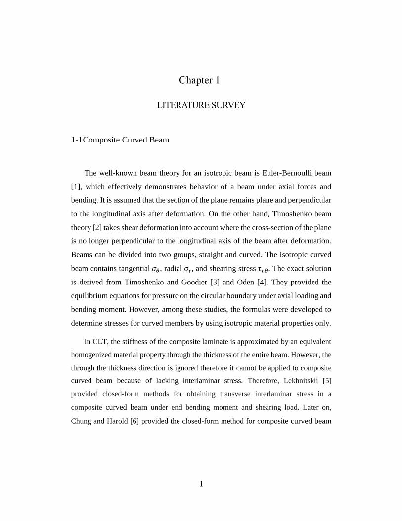
The well-known beam theory for an isotropic beam is Euler-Bernoulli beam

[1], which effectively demonstrates behavior of a beam under axial forces and

bending. It is assumed that the section of the plane remains plane and perpendicular

to the longitudinal axis after deformation. On the other hand, Timoshenko beam

theory [2] takes shear deformation into account where the cross-section of the plane

is no longer perpendicular to the longitudinal axis of the beam after deformation.

Beams can be divided into two groups, straight and curved. The isotropic curved

beam contains tangential 𝜎𝜃, radial σr, and shearing stress 𝜏𝑟𝜃. The exact solution

is derived from Timoshenko and Goodier [3] and Oden [4]. They provided the

equilibrium equations for pressure on the circular boundary under axial loading and

bending moment. However, among these studies, the formulas were developed to

determine stresses for curved members by using isotropic material properties only.

In CLT, the stiffness of the composite laminate is approximated by an equivalent

homogenized material property through the thickness of the entire beam. However, the

through the thickness direction is ignored therefore it cannot be applied to composite

curved beam because of lacking interlaminar stress. Therefore, Lekhnitskii [5]

provided closed-form methods for obtaining transverse interlaminar stress in a

composite curved beam under end bending moment and shearing load. Later on,

Chung and Harold [6] provided the closed-form method for composite curved beam

2

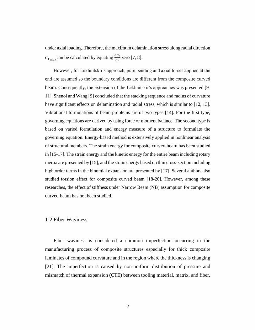
under axial loading. Therefore, the maximum delamination stress along radial direction

σrmaxcan be calculated by equating 𝑑𝜎𝑟

𝑑𝑟 zero [7, 8].

However, for Lekhnitskii’s approach, pure bending and axial forces applied at the

end are assumed so the boundary conditions are different from the composite curved

beam. Consequently, the extension of the Lekhnitskii’s approaches was presented [9-

11]. Shenoi and Wang [9] concluded that the stacking sequence and radius of curvature

have significant effects on delamination and radial stress, which is similar to [12, 13].

Vibrational formulations of beam problems are of two types [14]. For the first type,

governing equations are derived by using force or moment balance. The second type is

based on varied formulation and energy measure of a structure to formulate the

governing equation. Energy-based method is extensively applied in nonlinear analysis

of structural members. The strain energy for composite curved beam has been studied

in [15-17]. The strain energy and the kinetic energy for the entire beam including rotary

inertia are presented by [15], and the strain energy based on thin cross-section including

high order terms in the binomial expansion are presented by [17]. Several authors also

studied torsion effect for composite curved beam [18-20]. However, among these

researches, the effect of stiffness under Narrow Beam (NB) assumption for composite

curved beam has not been studied.

1-2 Fiber Waviness

Fiber waviness is considered a common imperfection occurring in the

manufacturing process of composite structures especially for thick composite

laminates of compound curvature and in the region where the thickness is changing

[21]. The imperfection is caused by non-uniform distribution of pressure and

mismatch of thermal expansion (CTE) between tooling material, matrix, and fiber.

3

This will cause longitudinal and transverse stresses in composite, including higher

matrix contraction and fiber buckling as stated by Kantharaju [22]. Parameters on

developing fiber waviness have been studied by Kugler and Moon [23]. They

concluded that the influence of holding cure temperature is insignificant, but the

cooling rate will affect the severity and the quantity of fiber waviness.

The concept of elastic moduli reduction for initial distortions of the

unidirectional reinforcing layers was first provided by Bolotin [31]. In his analysis,

Kirchhoff hypothesis was used to describe the deformation of thin layers or slightly

twisted plates with initial irregulations. In connection with the study of layered

reinforced media with random initial irregularities, reduction on the modulus of

elasticity in tension along the fibers of unidirectional glass-reinforced plastics (GRP)

is proposed by Tarnopol'skii et al. [32]. The shape of fiber irregularities is assumed

to be a sinusoidal function. Bažant [33] advanced their approach by taking into

account changes in wave amplitude due to radial forces. Three ideal cases of

unidirectional fiber distributions were discussed. The first one is parallel, uniformly

distributed fibers with sinusoidal curvature. The second one is not strictly parallel

distributed fibers with sinusoidal curvature. The third one is when fiber waviness

are equal in amplitude but in opposite directions.

Extensive investigations of stiffness loss due to fiber waviness was conducted

in [34-36]. Lo and Chim [37] predicted the compressive strength of unidirectional

composite with fiber waviness. Adams and Hyer [38] experimentally investigated

multi-directional composite laminates under static compression loading. They

observed that severe waviness induced a static strength reduction of 36 %, although

the fiber waviness occurred in 0° ply and accounted for only 20 % of the load-

carrying capacity of the laminate. Rai et al. [39] numerically investigated lamina

modulus as a function of fiber waviness, which is similar to [40-43]. They

concluded that fiber waviness, which occurs in 0° ply has significant influence on

4

stiffness reduction. If fiber waviness occurs in ±45° ply, the influence in stiffness

reduction is more pronounced in torsional cases than bending cases.

Fiber waviness can occur in either in-plane or out-of-plane for a laminated

beam [44]. The effects of out-of-plane fiber waviness for a lamina were further

investigated by Hsiao and Daniel [45-47]. Three types of fiber waviness are

considered including uniform, graded and localized fiber waviness. They

concluded that tensile and compressive elastic properties and nonlinear behavior in

composite materials can be significantly influenced by fiber waviness. Several

researchers applied numerical method for investigating effects of fiber waviness.

Seon [48] studied tape composite with fiber waviness by linear and nonlinear FE

analysis. The nonlinear interlaminar stress-strain relations can improve the

delamination onset prediction. He observed that the failure load for a rectangular

tape with small amplitude fiber waviness under tension is higher compared to fiber

waviness with large amplitude. Nikishkov et al. [49] conducted a numerical model

to investigate progressive fatigue damage in composites with fiber waviness.

However, most of analytical researches is not focused on out-plane fiber waviness

for a laminated composite beam. Therefore, the object of this research is to develop

a feasible and efficient approach to analyze composite curved beam with out-of-

plane fiber waviness.

There is a type of composites where fiber waviness is built-in by design,

namely textile [50] and braided composites [51]. The fiber waviness leads to same

general property effects such as modulus and strength reduction [52-55]. However,

it allows to produce composites with greatly improved properties in the transverse

direction and, in the case of 3D reinforcement, also in the out-of-plane direction. A

detailed review of the respective literature is beyond the scope of this work. It is

worth mentioning that application of analytical methods has led to accurate

5

estimates of stiffness properties of such materials as a function of fiber angulation

and is addressed in a number of works including in [56-58].

1-3 Composite Curved Beam with Delamination

Three principle failure models are often to be found in a laminated composite

– fiber failure, matrix cracking, and delamination [59]. Delamination is considered

as one of the dominant failure factors in composites and leads to substantial

stiffness loses [60, 61], and local compressive failure due to instability [62].

Delamination is driven by interlaminar stresses, Interlaminar Shear Stress (ILSS)

and Interlaminar Tensile Stress (ILTS). When ILSS or ILNS grows over the critical

value given from the material, the delamination starts to initiate and propagate.

There are several affects have impacts on interlaminar stresses, including stacking

sequence, Poisson’s ratio mismatch, ply thickness [63], and free-edge effect [64-

66]. The initiation of delamination usually occurs at the location with the highest

ILTS.

Another essential factor to describe initiation and propagation of delamination is

strain ERR. Double Cantilever Beam (DCB) test (ASTM D5228) [67] is the method

for measuring Mode-I fracture toughness, and End-Notched Flexure (ENF) test

(ASTM WK22949) [68] is the method for measuring Mode-II fracture toughness

experimentally. Mode-I and Mode-II delamination can be also predicted accurately

by analytical methods based on the plate theory and bridge-crack models [69-71]. Due

to limit cases can be applied for pure Mode-I and Mode-II fracture, a mixed-mode

approach based on non-linear and Timoshenko first-order shear theory is developed

[72] for a straight beam. Considering a beam with an initial curvature, Lu et al. [73]

considered a circumferential crack in composite curved beam under bending.

6

Superposition method of a perfect curved beam under bending and a cracked curved

beam subjected to opening radial stress acting on the crack interface was applied. They

assumed that if the crack is small and locates in the middle of the beam, the crack is

considered in pure Mode-I. Based on their observations, the strain ERR reaches the

maximum when the half crack angle approaches to 45°, and the strain ERR decreases

monotonically when the crack location approaches to outer curvature of the curved

beam. Moreover, they studied the strain ERR for a large crack using FE analysis. They

found that Mode-II becomes dominant when the crack tip reaches to 90° . This

conclusion is similar than the conclusion made by [74].

Roberta and Brian [75] developed an analytical approach based on bridged-

crack model which deals with mixed-mode delamination in composite curved beam

under bending. In their model, the strain ERR is calculated by considering the J-

integral along a path surrounding the crack tip. It can be observed that regarding less

small crack angle θc, strain ERR results using beam theory are accurate compared to

FE results. The similar conclusion is made by Bruno et al. [76]. They concluded that

as a matter of fact for a short crack, curved laminated beam theory is not appropriate.

The strain ERR value between their model and FE results are within 8 % error except

for very short crack, where θc < 5°. However, among their approaches, only a crack

which is symmetric with respect to the middle span of the curved beam can be applied.

Therefore, the objective of this study is to develop an analytical analysis for a

composite curved beam with a delamination locates in any arbitrary interface and

hoop location.

7

RESEARCH OBJECTIVES

Composite structures provide higher specific strength and stiffness than

structures composed of metallic materials. Among various applications, one of the

most important components are composite beams. Over the last three decades,

composite beams have been widely used in automobile and aerospace applications. In

aerospace industry, aircraft wings contain box structures which are typically assembled

of stringers and spars. A number of different cross-sections “I”, “C”, and “Z” are

considered, where the concept of composite curved beam is applied. While FE based

computational approaches have been developed and widely used to address various

types of composite structures, there is a need to develop more efficient and compact

analytical methods. Development of such approaches for curved beam structures is the

overarching goal of the present research. Three different approaches are applied to

analysis of composite beams including conventional beam, Wide Beam (WB) and

Narrow Beam (NB) assumptions. General beam method is derived from CLT which

takes in-plane properties into account. For WB, twisting curvature is allowed so

that𝑀𝑥𝑦 = 0. On the other hand, twisting curvature is suppressed for NB, and 𝑀𝑥𝑦 ≠

0 is induced.

The first objective of this research is to apply the NB assumptions to composite

curved beam. The formulation of axial and bending stiffness of composite curved beam

can yield very different results using different beam assumptions depends on the cross-

section of the beam. If the width to height ratio is small (w

t≪ 6), NB assumption has

to be applied.

The second objective is to predict stiffness reduction and stress variation in

composites curved beam due to out-of-plane local fiber waviness. Composite materials

8

have defects and imperfections such as fiber waviness, delamination, porosity, and

resin migration, which are caused by the manufacturing process [77]. Fiber waviness

often can be found in thick composites [78]. Several factors can cause this defect

including non-uniform cure pressure, resin shrinkage or pre-buckling. Fiber waviness

has an adverse influence on the mechanical properties. The tensile, compressive

strength, and fatigue life degrade significantly [79]. Most of the research focused on

fiber waviness is performed in unidirectional flat composites, but fiber waviness in

composite curved beam using analytical approaches is not addressed. The proposed

research aims to fill this void. A FE analysis will be conducted to verify results. If fiber

waviness is located near leg region of curved beam, the maximum tensile stress 𝜎𝑟 no

longer located in the middle span of the composite curved beam.

The third objective is to predict failure load of composite curved beam with

delamination under bending. In the past studies, the delamination can be only located

symmetrically with respect to the middle span of the composite curved beam. The

results show that the strain ERR results have good agreement compared with FE

analysis. However, for a short crack (θc < 5°), analytical results no longer satisfy the

numerical results. Therefore, this research aims to fill the void. In the present research,

we allow for a delamination which is not symmetric with respect to the middle span of

the composite curved beam and it can be located at any arbitrary interface.

9

OVERVIEW OF CLASSICAL LAMINATION THEORY

3-1 Lamina Stage

A Lamina contains fiber and matrix which is characterized as a single layer.

It is an orthotropic material with principal material axes in the fiber direction. In

lamina level, it is usually to consider material homogeneous, and average properties

is used in the analysis. This type of analysis is called micromechanics and

considered the unidirectional lamina as a quasi-homogeneous anisotropic material

with averaged stiffness and strength. A thin-walled unidirectional lamina is

generally under plane stress assumption. Stresses along the thickness direction are

assumed to be zeros, 𝜎3 = 𝜏13 = 𝜏23 = 0. The stress/strain relationship is further

reduced to

[

𝜎1𝜎2𝜏12] = [

𝑄11 𝑄12 0𝑄12 𝑄22 00 0 𝑄66

] [

𝜀1𝜀2𝑟12] (3-1)

where

Q11 =𝐸1

1 − 𝑣12𝑣21 , 𝑄22 =

𝐸21 − 𝑣12𝑣21

𝑄12 =𝑣12𝐸2

1 − 𝑣12𝑣21 , 𝑄66 = 𝐺12

(3-2)

𝐸1 is Young’s modulus along 1-direction (fiber direction).

10

𝐸2 is Young’s modulus along 2-direction.

𝐺12 is shear modulus along 1-2 plan.

𝑣12 is Poisson’s ratio associated with loading in 1-direction and produced strain in

2-direction.

𝑣21 is Poisson’s ratio associated with loading in 2-direction and produced strain in

1-direction.

For a general anisotropic material, 21 material constants exhibit

extension/shear coupling behavior. For a general orthotropic material, 9 material

constants exhibit no extension/shear coupling behavior. If a thin orthotropic

material is considered, only 4 material constants required to fully describe material

behavior of a 2-D orthotropic material, 𝐸1, 𝐸2, 𝐺12, and 𝑣12. In viewing Eqs. (3-1),

[𝑄] matrix is so-called the reduced stiffness matrix, no shear strain is induced when

σ1 is applied. In addition, no in-plane strains are induced if τ12 is applied. This

implies that for 0° lamina, where no extension/shear coupling are presented.

3-2 Stress Transformation

Normally, the lamina principal axes (1 and 2) do not coincide with the

loading axes (x and y). The stress components referred to the principal axes can be

transferred in terms of loading axes. The following Eqs. (3-3) shows stress

transformation from 1-2 axes to x-y axes.

[

𝜎𝑥𝜎𝑦𝜏𝑥𝑦

] = [𝑇𝜎(−𝜃)] [

𝜎1𝜎2𝜏12] (3-3)

11

where

[𝑇𝜎(𝜃)] = [𝑚2 𝑛2 2𝑚𝑛𝑛2 𝑚2 −2𝑚𝑛−𝑚𝑛 𝑚𝑛 𝑚2 − 𝑛2

]

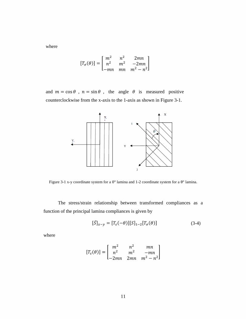
and 𝑚 = cos 𝜃 , 𝑛 = sin 𝜃 , the angle 𝜃 is measured positive

counterclockwise from the x-axis to the 1-axis as shown in Figure 3-1.

Figure 3-1 x-y coordinate system for a 0° lamina and 1-2 coordinate system for a θ° lamina.

The stress/strain relationship between transformed compliances as a

function of the principal lamina compliances is given by

[𝑆]𝑥−𝑦 = [𝑇𝜀(−𝜃)][𝑆]1−2[𝑇𝜎(𝜃)] (3-4)

where

[𝑇𝜀(𝜃)] = [𝑚2 𝑛2 𝑚𝑛𝑛2 𝑚2 −𝑚𝑛

−2𝑚𝑛 2𝑚𝑛 𝑚2 − 𝑛2]

12

[𝑆]1−2 =

[ 1

𝐸1−𝑣12𝐸2

0

−𝑣12𝐸2

1

𝐸20

0 01

𝐺12]

The relationship of stiffness matrix in x-y coordinate system can be transformed

to 1-2 coordinate system in terms of basic material constants 𝐸1, 𝐸2, 𝑣12, and 𝐺12.

[��]𝑥−𝑦 = [𝑇𝜎(−𝜃)][𝑄]1−2[𝑇𝜀(𝜃)] (3-5)

3-3 Laminate Stage (Classical Lamination Theory)

The overall structural behavior of multidirectional laminate is a function of

stacking sequence and material properties. The Classical Lamination Theory (CLT)

for a multidirectional laminate predicts the behavior of the laminate based on

several assumptions. First, the laminate is thin which means the lateral dimension

is much larger than its thickness direction. Therefore, the plane stress assumption

has to be followed, 𝜎𝑧 = 𝜏𝑥𝑧 = 𝜏𝑦𝑧 = 0 . Second, displacements are small

compared with the thickness of the laminate and displacements are continuous

through the laminate. Third, cross-section remains normal to the middle surface

after deformation, 𝛾𝑥𝑧 = 𝛾𝑦𝑧 = 0 . Also, the normal distances from the middle

surface remain constant, that is 𝜀𝑧 = 0. In general, each lamina and the entire

laminate behave linearly elastic.

The displacements of the mid-plane are function of x and y:

𝑢0 = 𝑢0(𝑥, 𝑦) (3-6)

13

𝑣0 = 𝑣0(𝑥, 𝑦)

𝑤0 = 𝑤0(𝑥, 𝑦)

where 𝑢0, 𝑣0 and 𝑤0 are displacements in the x, y, and z directions, respectively.

The reference plane of a laminated plate locates at the mid plane of the plate. In

general,

𝑢 = 𝑢0 − 𝑧𝜕𝑤

𝜕𝑥

𝑣 = 𝑣0 − 𝑧𝜕𝑤

𝜕𝑦

(3-7)

where z is the through thickness coordinate.

A linear strain function across the thickness is assumed based on linear

elastic behavior of the laminate. The strains at any given point can be expressed as

functional of the reference plane strains and the laminate curvatures.

[

𝜀𝑥𝜀𝑦𝛾𝑥𝑦] = [

𝜀𝑥0

𝜀𝑦0

𝛾𝑥𝑦0

] + 𝑧 [

𝐾𝑥𝐾𝑦𝐾𝑥𝑦

] (3-8)

𝜀𝑥0, 𝜀𝑦

0, 𝛾𝑥𝑦0 , 𝐾𝑥 , 𝐾𝑦 and 𝐾𝑥𝑦 are mid-plane strains and curvatures can be expressed

as

𝜀𝑥0 =

𝜕𝑢0𝜕𝑥

𝜀𝑦0 =

𝜕𝑣0𝜕𝑦

𝛾𝑥𝑦0 =

𝜕𝑢0𝜕𝑦

+𝜕𝑣0𝜕𝑥

(3-9)

14

𝐾𝑥 = −𝜕2𝑤

𝜕𝑥2

𝐾𝑦 = −𝜕2𝑤

𝜕𝑦2

𝐾𝑥𝑦 = −2𝜕2𝑤

𝜕𝑥𝜕𝑦

Once strain in 𝑘𝑡ℎ layer is obtained, the stresses in the 𝑘𝑡ℎ layer can be written as

[


]

𝑘𝑡ℎ

= [��𝑥−𝑦]𝑘𝑡ℎ ([

𝜀𝑥0

𝜀𝑦0

𝛾𝑥𝑦0

] + 𝑧𝑘𝑡ℎ [


]) (3-10)

Based on Eqs. (3-10), even though the strain is linearly varied through the

thickness direction of the laminate, the stress in each layer is discontinuous due to

the varied transformed stiffness matrix [��𝑥−𝑦]𝑘𝑡ℎ. However, analyzing each layer

individually is a cumbersome task. Because of the discontinuous variation of

stresses, it is convenient to deal with the plate forces and plate moment instead of

identifying individual layer. In laminate stage, the total force and moment resultants

can be obtained by summing the effects for all layers as shown below.

[

𝑁𝑥𝑁𝑦𝑁𝑥𝑦

] = ∑∫ [


]

𝑘𝑡ℎ

𝑑𝑧𝑧𝑘

𝑧𝑘−1

𝑛

𝑘=1

[

𝑀𝑥

𝑀𝑦

𝑀𝑥𝑦

] = ∑∫ [


]

𝑘𝑡ℎ

𝑧 𝑑𝑧𝑧𝑘

𝑧𝑘−1

𝑛

𝑘=1

(3-11)

where 𝑧𝑘 and 𝑧𝑘−1 are the z-coordinates of the upper and lower surface in 𝑘𝑡ℎ layer.

After integration, the plane force and moment resultants can be expressed as

15

[

𝑁𝑥𝑁𝑦𝑁𝑥𝑦

] = [𝐴] [

𝜀𝑥0

𝜀𝑦0

𝛾𝑥𝑦0

] + [𝐵] [


]

[

𝑀𝑥

𝑀𝑦

𝑀𝑥𝑦

] = [𝐵] [

𝜀𝑥0

𝜀𝑦0

𝛾𝑥𝑦0

] + [𝐷] [


]

(3-12)

where

[𝐴] = ∑[��𝑥−𝑦]𝑘𝑡ℎ(𝑧𝑘 − 𝑧𝑘−1)

𝑛

𝑘=1

𝑢𝑛𝑖𝑡 = 𝑙𝑏/𝑖𝑛

[𝐵] =1

2∑[��𝑥−𝑦]𝑘𝑡ℎ

(𝑧𝑘2 − 𝑧𝑘−1

2 )

𝑛

𝑘=1

𝑢𝑛𝑖𝑡 = 𝑙𝑏

[𝐷] =1

3∑[��𝑥−𝑦]𝑘𝑡ℎ

(𝑧𝑘3 − 𝑧𝑘−1

3 ) 𝑢𝑛𝑖𝑡 = 𝑙𝑏 − 𝑖𝑛

𝑛

𝑘=1

(3-13)

In viewing Eqs. (3-13), [𝐴], [𝐵] and [𝐷] matrix are functions of geometry, material

properties and stacking sequence. They are the averaging elastic stiffness. [𝐴] is an

extensional stiffness matrix relating in-plane loads to in-plane strains. [𝐵] is an

extensional-bending coupling stiffness matrix relating in-plane load to curvatures

and moments to in-plane strains. [𝐷] is a bending stiffness matrix. The relationship

between force and moment resultants to the mid-plane strains and curvatures is

shown below.

[��]6𝑥1

= [𝐴 𝐵𝐵 𝐷

]6𝑥6

[𝜀0

𝐾]6𝑥1

(3-14)

16

[𝜀0

𝐾]6𝑥1

= [𝑎 𝑏𝑏 𝑑

]6𝑥6

[��]6𝑥1

[𝑎 𝑏𝑏 𝑑

]6𝑥6

= [𝐴 𝐵𝐵 𝐷

]−1

6𝑥6

where [��] = 𝑁 ,[��] = 𝑀 is shown in Eqs. (3-11). If mechanical loading and

temperature loading are both considered, [��] = [𝑁] + [𝑁𝑇] and [��] = [𝑀] +

[𝑀𝑇], where thermal induced loads [𝑁𝑇] and thermal induced moments [𝑀𝑇] is

written as:

[𝑁𝑇] = ∆𝑇∑ [��𝑥−𝑦]𝑘𝑡ℎ[𝛼𝑥−𝑦 ]𝑘𝑡ℎ(𝑧𝑘 − 𝑧𝑘−1)

𝑛

𝑘=1

[𝑀𝑇] =∆𝑇

2∑ [��𝑥−𝑦]𝑘𝑡ℎ[𝛼𝑥−𝑦 ]𝑘𝑡ℎ

(𝑧𝑘2 − 𝑧𝑘−1

2 )𝑛

𝑘=1

(3-15)

where 𝛼𝑥−𝑦 is the Coefficient of Thermal Expansion (CTE) and ∆𝑇 is the

temperature difference.

17

STIFFNESS AND STRESS INVESTIGATION OF COMPOSITE

CURVED BEAM

4-1 Stiffness Model Formulation for Composite Curved Beam

The curved beam geometry shown in Figure 4-1 represents a rectangular

cross-section with a mean radius 𝑅𝑚 where 𝑅𝑚 = (𝑅𝑜 + 𝑅𝑖)/2, and 𝑅𝑜 is the outer

radius and 𝑅𝑖 is the inner radius of the curved beam. Beams usually are slender, and

its dimension along the x-direction is greater than the other dimensions along y and

z directions. The longitudinal axis is in the x or 𝜃 direction. The out-of-plane axis

is in the z or r direction.

Assume line 𝑝𝑝′ is the mid-axis of the curved beam. In the 𝑘𝑡ℎ layer, the

elongation after deformation is (𝑅𝑚 + 𝑧)𝑑𝜃 𝜀𝜃 . This elongation can be further

describe in terms of mid-plane strain, 𝜀0 , and curvature K, which is (𝑅𝑚 +

𝑧)𝑑𝜃 (𝜀0 + 𝑧 𝐾). By equating above equations, the strain in any given point along

𝜃 direction can be expressed as

𝜀𝜃 =𝑅𝑚

𝑅𝑚 + 𝑧(𝜀0 + 𝑧 𝐾) (4-1)

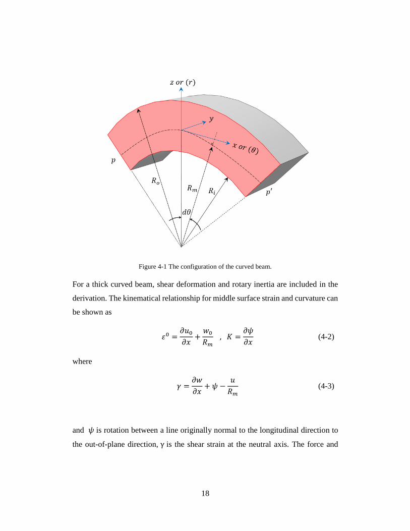
18

Figure 4-1 The configuration of the curved beam.

For a thick curved beam, shear deformation and rotary inertia are included in the

derivation. The kinematical relationship for middle surface strain and curvature can

be shown as

𝜀0 =𝜕𝑢0𝜕𝑥

+𝑤0𝑅𝑚

, 𝐾 =𝜕𝜓

𝜕𝑥 (4-2)

where

𝛾 =𝜕𝑤

𝜕𝑥+ 𝜓 −

𝑢

𝑅𝑚 (4-3)

and 𝜓 is rotation between a line originally normal to the longitudinal direction to

the out-of-plane direction, γ is the shear strain at the neutral axis. The force and

19

moment resultants of the curved beam can be obtained by integrating stresses over

the thickness of the beam.

[𝑁] = ∑ ∫ [��𝑥−𝑦]𝑘𝑡ℎ

𝑧𝑘

𝑧𝑘−1

𝑛

𝑘=1

𝑅𝑚𝑅𝑚 + 𝑧

(𝜀0 + 𝑧 𝐾) 𝑑𝑧 = [Ac]𝜀0 + [𝐵𝑐]𝐾

[𝑀] = ∑ ∫ [��𝑥−𝑦]𝑘𝑡ℎ

𝑧𝑘

𝑧𝑘−1

𝑛

𝑘=1

𝑅𝑚𝑅𝑚 + 𝑧

(𝜀0 + 𝑧 𝐾) 𝑧 𝑑𝑧 = [Bc]𝜀0 + [𝐷𝑐]𝐾

(4-4)

The averaging stiffness for a composite curved beam [Ac], [Bc], and [Dc] matrix

can be expressed as

[𝐴𝑐] = 𝑅𝑚∑[��𝑥−𝑦]𝑘𝑡ℎ ln𝑅𝑚 + 𝑧𝑘𝑅𝑚 + 𝑧𝑘−1

𝑛

𝑘=1

[𝐵𝑐] = 𝑅𝑚∑[��𝑥−𝑦]𝑘𝑡ℎ

𝑛

𝑘=1

[(𝑧𝑘 − 𝑧𝑘−1) − 𝑅𝑚 ln𝑅𝑚 + 𝑧𝑘𝑅𝑚 + 𝑧𝑘−1

]

[𝐷𝑐] = 𝑅𝑚∑[��𝑥−𝑦]𝑘𝑡ℎ [1

2(𝑧𝑘2 − 𝑧𝑘−1

2 ) − 𝑅𝑚(𝑧𝑘 − 𝑧𝑘−1) + 𝑅𝑚2 ln

𝑅𝑚 + 𝑧𝑘𝑅𝑚 + 𝑧𝑘−1

]

𝑛

𝑘=1

(4-5)

The shear stiffness [𝐺𝐴 𝑐] can be also describe as functional of 𝑅𝑚 :

[𝐺𝐴 𝑐] = 𝑘𝑠𝑅𝑚∑(𝐺13 cos2 𝜃𝑘) ln


𝑛

𝑘=1

(4-6)

where ks is the shear correction factor, typically taken as 5/6 for rectangular cross-

section. θk is the stacking sequence at the kth layer. All the derivation can be found

in detail from [13, 15, and 80].

20

4-2 Modified Stiffness Approach for Composite Beam

The cross-section of a beam can be categorized into three groups, general,

wide, and narrow section. For a general beam which does not take the width to

height ratio into account, since the twisting curvature 𝐾𝑥𝑦 is allowed, no twisting

moment 𝑀𝑥𝑦 is induced. Therefore, the constitutive equation can be expressed as

[𝜀𝑥0

𝐾𝑥] = [

𝑎11 𝑏11𝑏11 𝑑11

] [𝑁𝑥𝑀𝑥] (4-7)

where 𝑁𝑥 is an applied force per unit width along x-direction and 𝑀𝑥 is an applied

moment per unit width. The axial stiffness is 1

𝑎11 , and the bending stiffness is

1

𝑑11.

4.2.1. Wide Beam (WB)

If the width to height ratio is too small or too large, extra modifications

should be considered. Considering a flat plate where the width to height ratio

usually greater than 6, the lateral curvature, 𝐾𝑦 is suppressed because of the flat

cross-section under bending as shown in Figure 4-2. Since 𝑁𝑥 and 𝑀𝑥 are applied,

𝜀𝑥0 ≠ 0 and 𝐾𝑥 ≠ 0. Moreover, due to flat plate geometry of the cross-section, mid-

plane strains and curvatures in transverse direction are equal to zero. Hence, the

resultants forces and moment in y and shear direction are induced.

𝜀𝑦0 = 𝛾𝑥𝑦

0 = 𝐾𝑦 = 𝐾𝑥𝑦 = 0

𝑁𝑦 ≠ 0, 𝑁𝑥𝑦 ≠ 0, 𝑀𝑦 ≠ 0, 𝑀𝑥𝑦 ≠ 0

(4-8)

21

The constitutive equation of a beam with wide cross-section can be expressed as

[𝑁𝑥𝑀𝑥] = [

𝐴11 𝐵11𝐵11 𝐷11

] [𝜀𝑥0

𝐾𝑥]

[𝜀𝑥0

𝐾𝑥] = [

𝐴11 𝐵11𝐵11 𝐷11

]−1

[𝑁𝑥𝑀𝑥]

𝐴𝑥 = 𝐴11 −𝐵112

𝐷11, 𝐵𝑥 = 𝐵11 −

𝐴11𝐷11𝐵11

, 𝐷𝑥 = 𝐷11 −𝐵112

𝐴11

(4-9)

where 𝐴𝑥 is axial stiffness, 𝐵𝑥 is coupling stiffness, and 𝐷𝑥 is bending stiffness.

In addition, the resultant force and moment in the transverse direction can

be also obtained.

[ 𝑁𝑦𝑁𝑥𝑦𝑀𝑦

𝑀𝑥𝑦]

= [

𝐴12 𝐵12𝐴16 𝐵16𝐵12 𝐷12𝐵16 𝐷16

] [𝐴11 𝐵11𝐵11 𝐷11

]−1

[𝑁𝑥𝑀𝑥] (4-10)

Figure 4-2 Deformed shape of laminated beam under pure bending with narrow and wide cross-

sections.

22

4.2.2. Narrow Beam (NB)

If the width to height ratio of the cross-section is small as shown in Figure

4-2, the lateral curvature 𝐾𝑦 is induced due to the effect of Poisson’s ratio. For a

beam under a bending moment 𝑀𝑥 across the width of the beam, 𝑤, 𝑀𝑥𝑦 is induced.

Since the loads per unit width is employed in the lamination theory, we have

𝜀𝑦0 ≠ 0, 𝛾𝑥𝑦

0 ≠ 0, 𝐾𝑦 ≠ 0, 𝐾𝑥𝑦 = 0

𝑁𝑦 = 0, 𝑁𝑥𝑦 = 0, 𝑀𝑦 = 0, 𝑀𝑥𝑦 ≠ 0

(4-11)

The overall 6 by 6 stiffness matrix in Eqs. (3-14) can be simplified to 3 by 3 matrix

under the above assumptions.

[𝜀𝑥0

𝐾𝑥𝐾𝑥𝑦

] = [

𝑎11 𝑏11 𝑏16𝑏11 𝑑11 𝑑16𝑏16 𝑑16 𝑑66

] [

𝑁𝑥𝑀𝑥

𝑀𝑥𝑦

] (4-12)

𝑀𝑥𝑦 can be expressed in terms of 𝑁𝑥 and 𝑀𝑥 due to suppressed curvature 𝐾𝑥𝑦.

𝑀𝑥𝑦 = −𝑏16𝑑66

𝑁𝑥 −𝑑16𝑑66

𝑀𝑥 (4-13)

Substituting Eqs. (4-13) back to (4-12), the mid-plane strain and curvature along

the x-direction are

𝜀𝑥0 = (𝑎11 −

𝑏162

𝑑66)𝑁𝑥 + (𝑏11 −

𝑏16𝑑16𝑑66

)𝑀𝑥

𝐾𝑥 = (𝑏11 −𝑏16𝑑16𝑑66

)𝑁𝑥 + (𝑑11 −𝑑162

𝑑66)𝑀𝑥

(4-14)

23

𝑎∗ = 𝑎11 −𝑏162

𝑑66, 𝑏∗ = 𝑏11 −

𝑏16𝑑16𝑑66

, 𝑑∗ = 𝑑11 −𝑑162

𝑑66

In viewing Eqs. (4-14), the axial stiffness is obtained if only 𝑁𝑥 is applied. Also,

the bending stiffness is obtained if only 𝑀𝑥 is applied. Thus, for bending case, 𝑁𝑥 =

0, and for tension case, 𝑀𝑥 = 0. The axial stiffness 𝐴𝑥 and bending stiffness 𝐷𝑥 for

a composite beam with narrow cross-section are shown below.

𝐴𝑥 =𝑑∗

𝑎∗𝑑∗ − 𝑏∗2, 𝐵𝑥 = −

𝑏∗

𝑎∗𝑑∗ − 𝑏∗2, 𝐷𝑥 =

𝑑∗

𝑎∗𝑑∗ − 𝑏∗2 (4-15)

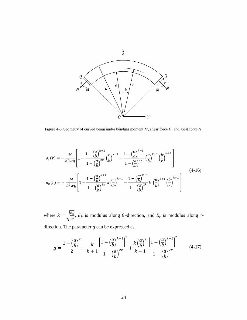
4-3 Ply-Stress Investigation

In this section, two approaches are discussed for investigating stress

distribution for the composite curved beam under bending. The first approach is

developed by Lekhnitskii [5] and extended by William [8]. Figure 4-3 shows a

curved beam subjected to shear force 𝑄, axial force 𝑁, and bending moment 𝑀.

The outer radius of the curved beam is denoted as b, and the inner radius of the

curved beam is denoted as a. r is the distance from the center point O to any radial

location of the curved beam. The width of the curved beam is denoted as w. If the

composite material of the curved beam is assumed as continuous anisotropic

material, the radial stress, tangential stress, and shear stress induced in the curved

beam under end bending moment can be expressed as

24

Figure 4-3 Geometry of curved beam under bending moment 𝑀, shear force 𝑄, and axial force 𝑁.

𝜎𝑟(𝑟) = −𝑀

𝑏2𝑤𝑔[1 −

1 − (𝑎𝑏)

𝑘+1

1 − (𝑎𝑏)

2𝑘 (𝑟

𝑏)𝑘−1

−1 − (

𝑎𝑏)

𝑘−1

1 − (𝑎𝑏)

2𝑘 (𝑎

𝑏)𝑘+1

(𝑏

𝑟)𝑘+1

]

𝜎𝜃(𝑟) = − 𝑀

𝑏2𝑤𝑔[1 −

1 − (𝑎𝑏)

𝑘+1

1 − (𝑎𝑏)

2𝑘 𝑘 (𝑟

𝑏)𝑘−1

−1− (

𝑎𝑏)

𝑘−1

1 − (𝑎𝑏)

2𝑘 𝑘 (𝑎

𝑏)𝑘+1

(𝑏

𝑟)𝑘+1

]

(4-16)

where 𝑘 = √𝐸𝜃

𝐸𝑟, 𝐸𝜃 is modulus along 𝜃 -direction, and 𝐸𝑟 is modulus along r-

direction. The parameter g can be expressed as

𝑔 =1 − (

𝑎𝑏)2

2−

𝑘

𝑘 + 1

[1 − (𝑎𝑏)𝑘+1

]2

1 − (𝑎𝑏)2𝑘 +

𝑘 (𝑎𝑏)2

𝑘 − 1 [1 − (

𝑎𝑏)𝑘−1

]2

1 − (𝑎𝑏)2𝑘 (4-17)

25

It is noticing that no shear stress 𝜏𝑟𝜃 is induced for a composite curved beam under

bending. In addition, both 𝜎𝑟 and 𝜎𝜃 are independent of 𝜃 based on Eqs. (4-16).

The stress induced in the composite curved beam due to the end shear force

𝑄 can be written as

𝜎𝑟(𝑟, 𝜃) =𝑄

𝑏𝑤𝑔1

𝑏

𝑟[(𝑟

𝑏)𝛽

+ (𝑎

𝑏)𝛽

(𝑏

𝑟)𝛽

− 1 − (𝑎

𝑏)𝛽

] sin 𝜃

𝜎𝜃(𝑟, 𝜃) =𝑄

𝑏𝑤𝑔1

𝑏

𝑟[(1 + 𝛽) (

𝑟

𝑏)𝛽

+ (1 − 𝛽) (𝑏

𝑟)𝛽

(𝑎

𝑏)𝛽

− 1 − (𝑎

𝑏)𝛽

] sin 𝜃

𝜏𝑟𝜃(𝑟, 𝜃) =𝑄

𝑏𝑤𝑔1

𝑏

𝑟 [(𝑟

𝑏)𝛽

+ (𝑎

𝑏)𝛽

(𝑏

𝑟)𝛽

− 1 − (𝑎

𝑏)𝛽

] cos 𝜃

(4-17)

where

𝛽 = √1 +𝐸𝜃𝐸𝑟(1 − 2𝑣𝑟𝜃) +

𝐸𝜃𝐺𝑟𝜃

𝑔1 =2

𝛽 [1 − (

𝑎

𝑏)𝛽

] + [1 + (𝑎

𝑏)𝛽

] ln𝑎

𝑏

(4-18)

and 𝐺𝑟𝜃 is shear modulus and 𝑣𝑟𝜃 is Poisson’s ratio.

It is noticing that radial stress, tangential stress, and shear stress are functional of 𝑟

and 𝜃. For isotropic material, the anisotropic parameter 𝛽 = 2.

The second approach is provided by Gonz alez-Cantero et al. [81, 82]. The

CLT approach can provide stresses in 𝜃 and y directions under bending moment

and axial forces for a composite curved beam. However, it is not capable to

compute interlaminar radial stress 𝜎𝑟 using CLT. Therefore, they provided an

26

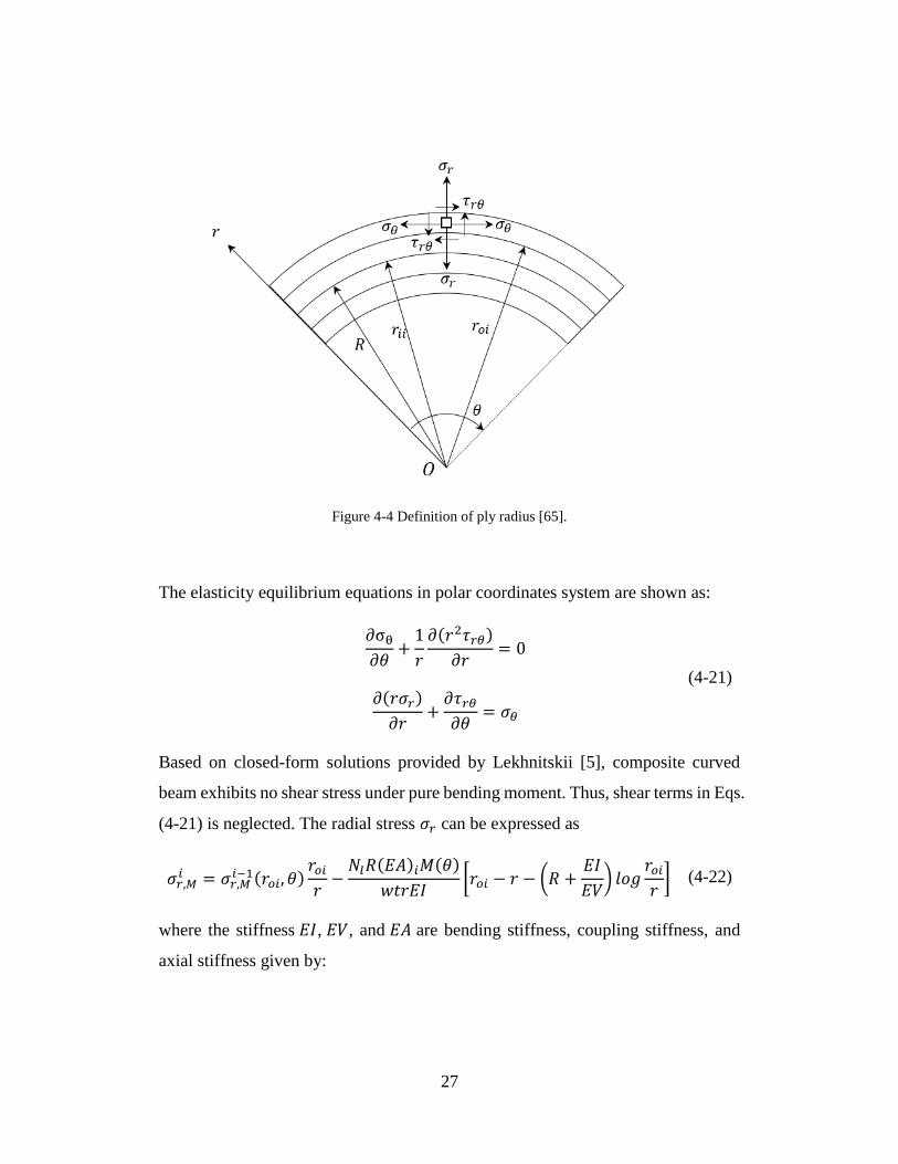
analytical model to aim this void. A cylindrical coordinate system with radius r and

the angle 𝜃 is shown in Figure 4-4, where R is the medium radius, 𝑟𝑖𝑖 and 𝑟𝑜𝑖 are

the inner and outer radius of the 𝑖𝑡ℎ ply. Substituting Eqs. (4-5) into (3-14), the mid-

plane strains and curvatures can be computed. For the bending case, �� = 0.

[𝜀0

𝐾]6𝑥1

= [𝑎𝑐 𝑏𝑐𝑏𝑐 𝑑𝑐

]6𝑥6

[��]6𝑥1

(4-19)

where

[𝑎𝑐 𝑏𝑐𝑏𝑐 𝑑𝑐

] = [𝐴𝑐 𝐵𝑐𝐵𝑐 𝐷𝑐

]−1

The strains in any radial location can be obtained using Eqs. (3-8), and the

tangential stress 𝜎𝜃 in the 𝑘𝑡ℎ ply can be further calculated using stress/strain

relationship in Eqs. (3-1).

[

𝜎𝜃𝜎𝑦𝜏𝑦𝜃

]

𝑘𝑡ℎ

= [

��11 ��12 ��16��12 ��22 ��16��16 ��26 ��66

]

𝑘𝑡ℎ

([

𝜀𝜃0

𝜀𝑦0

𝛾𝑦𝜃0

] + 𝑧 [

𝐾𝜃𝐾𝑦𝐾𝜃𝑦

]) (4-20)

It is noticing that only in-plane (𝜃, y) stresses are obtained using CLT due to plane

stress assumption as shown in Eqs. (4-20) where ��16 and ��26 are coupling terms

due to Poisson’s ratio. Once the tangential stress 𝜎𝜃 is obtained, the out-of-plane

stresses 𝜎𝑟 and 𝜏𝑟𝜃 can be computed due to equilibrium.

27

Figure 4-4 Definition of ply radius [65].

The elasticity equilibrium equations in polar coordinates system are shown as:

∂σθ𝜕𝜃

+1

𝑟

𝜕(𝑟2𝜏𝑟𝜃)

𝜕𝑟= 0

∂(𝑟𝜎𝑟)

𝜕𝑟+𝜕𝜏𝑟𝜃𝜕𝜃

= 𝜎𝜃

(4-21)

Based on closed-form solutions provided by Lekhnitskii [5], composite curved

beam exhibits no shear stress under pure bending moment. Thus, shear terms in Eqs.

(4-21) is neglected. The radial stress 𝜎𝑟 can be expressed as

𝜎𝑟,𝑀𝑖 = 𝜎𝑟,𝑀

𝑖−1(𝑟𝑜𝑖, 𝜃)𝑟𝑜𝑖𝑟−𝑁𝑙𝑅(𝐸𝐴)𝑖𝑀(𝜃)

𝑤𝑡𝑟𝐸𝐼[𝑟𝑜𝑖 − 𝑟 − (𝑅 +

𝐸𝐼

𝐸𝑉) 𝑙𝑜𝑔

𝑟𝑜𝑖𝑟] (4-22)

where the stiffness 𝐸𝐼, 𝐸𝑉, and 𝐸𝐴 are bending stiffness, coupling stiffness, and

axial stiffness given by:

28

𝐸𝐼 =∆𝑤

𝐴𝑐, 𝐸𝑉 =

∆𝑤

𝐵𝑐, 𝐸𝐴 =

∆𝑤

𝐷𝑐, ∆= 𝐴𝑐𝐷𝑐 − 𝐵𝑐

2 (4-23)

The stiffness (𝐸𝐴)𝑖 is axial stiffness for a single ply, (𝐸𝐴)𝑖 = 𝐸𝐴/𝑁𝑝, 𝑁𝑝 is total

number of plies for the composite curved beam. It should be noted that the radial

stress 𝜎𝑟,𝑀𝑖 depends on the previous ply 𝑖 − 1 . Therefore, initialize 𝜎𝑟

0 with

boundary condition is necessary and given by 𝜎𝑟𝑀0 (𝑟𝑖1, 𝜃) = 0.

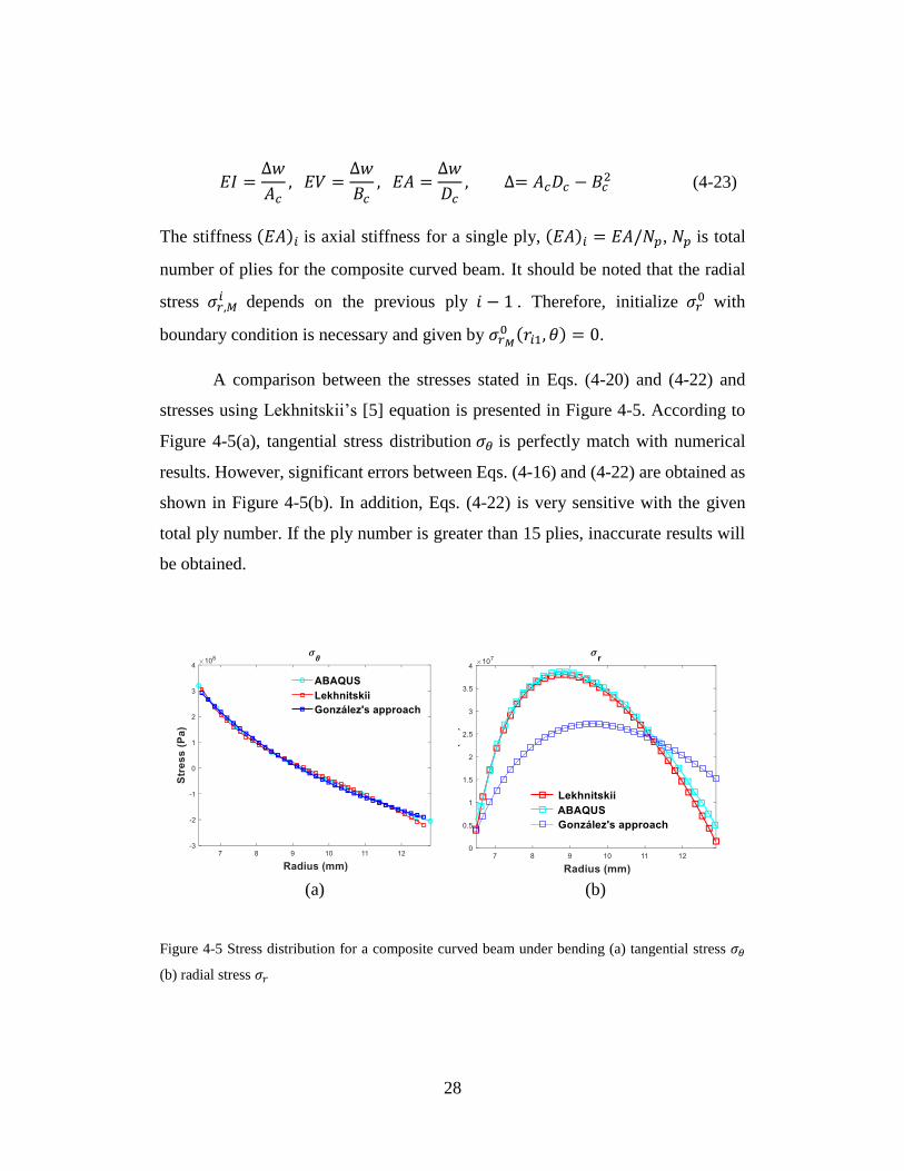
A comparison between the stresses stated in Eqs. (4-20) and (4-22) and

stresses using Lekhnitskii’s [5] equation is presented in Figure 4-5. According to

Figure 4-5(a), tangential stress distribution 𝜎𝜃 is perfectly match with numerical

results. However, significant errors between Eqs. (4-16) and (4-22) are obtained as

shown in Figure 4-5(b). In addition, Eqs. (4-22) is very sensitive with the given

total ply number. If the ply number is greater than 15 plies, inaccurate results will

be obtained.

Figure 4-5 Stress distribution for a composite curved beam under bending (a) tangential stress 𝜎𝜃

(b) radial stress 𝜎𝑟

(a) (b)

29

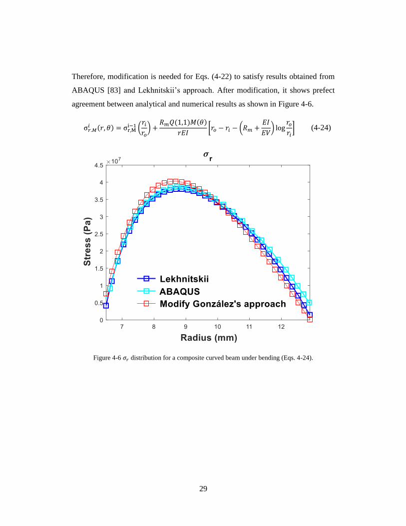
Therefore, modification is needed for Eqs. (4-22) to satisfy results obtained from

ABAQUS [83] and Lekhnitskii’s approach. After modification, it shows prefect

agreement between analytical and numerical results as shown in Figure 4-6.

σ𝑟.𝑀𝑖 (𝑟, 𝜃) = σr,M

i−1 (𝑟𝑖𝑟𝑜) +

𝑅𝑚𝑄(1,1)𝑀(𝜃)

𝑟𝐸𝐼[𝑟𝑜 − 𝑟𝑖 − (𝑅𝑚 +

𝐸𝐼

𝐸𝑉) log

𝑟𝑜𝑟𝑖] (4-24)

Figure 4-6 𝜎𝑟 distribution for a composite curved beam under bending (Eqs. 4-24).

30

4-4 Effective Stiffness Results and Discussion

In this study, three different beam assumptions due to width to height ratio

are discussed including general, wide, and narrow cross-section beams. A

parameter study is presented in this section to describe behaviors of the beam using

general, wide, and narrow assumptions, respectively. The inner radius of the

composite curved beam is 6.4 mm and the outer radius is 12.988 mm. The width of

the beam is 12.7 mm. Therefore, the mean radius 𝑅𝑚 is 9.694 mm and the total

thickness of the beam is 6.588 mm, which means it contains 36 plies and the ply

thickness is 0.183 mm for IM7/8552 material. The material properties for IM7/8552

[84] are:

E1 = 157 GPa E2 = 8.96 GPA E3 = 8.96 GPa

G12 = 5.08 GPa G23 = 2.99 GPa G13 = 5.08 GPa

v12 = 0.32 v23 = 0.5 v13 = 0.32

where E1, E2, and E3 are the Young’s moduli of the composite lamina along the

material coordinates. 𝐺12, 𝐺23, 𝐺13 and are the Shear moduli and 𝜈12 , 𝜈23, and 𝜈13

are Poisson’s ratio with respect to the 1-2, 2-3 and 1-3 planes, respectively.

31

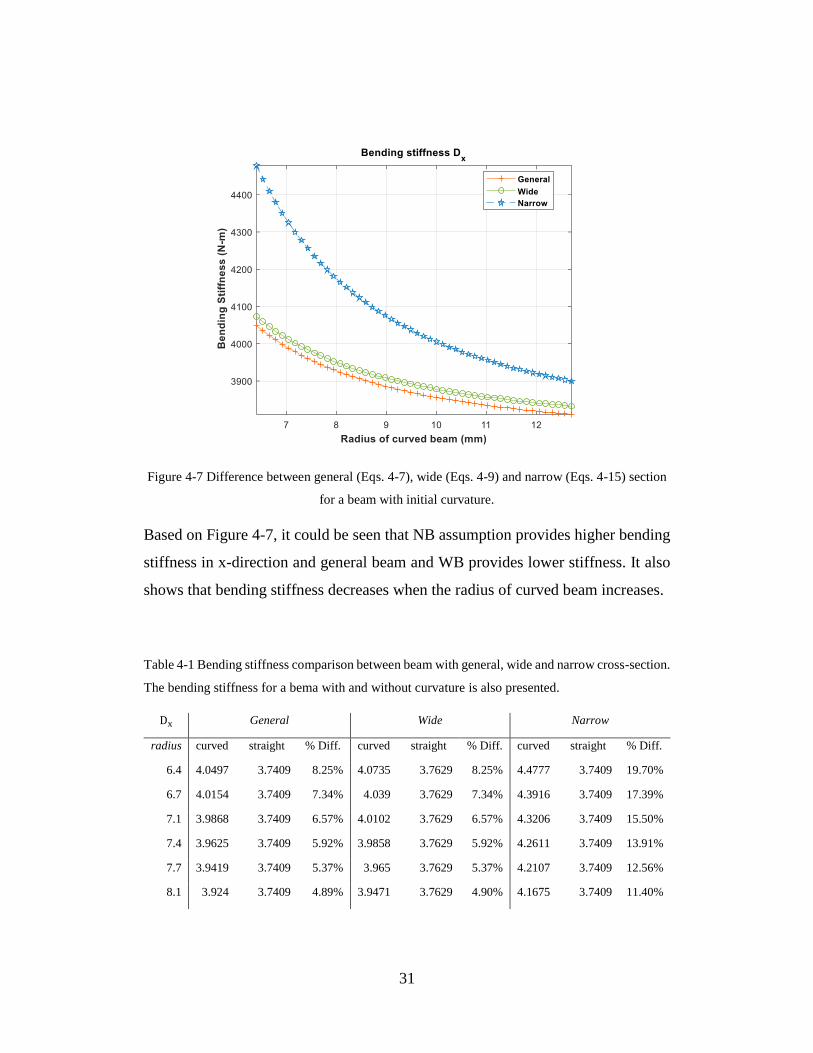
Figure 4-7 Difference between general (Eqs. 4-7), wide (Eqs. 4-9) and narrow (Eqs. 4-15) section

for a beam with initial curvature.

Based on Figure 4-7, it could be seen that NB assumption provides higher bending

stiffness in x-direction and general beam and WB provides lower stiffness. It also

shows that bending stiffness decreases when the radius of curved beam increases.

Table 4-1 Bending stiffness comparison between beam with general, wide and narrow cross-section.

The bending stiffness for a bema with and without curvature is also presented.

Dx General Wide Narrow

radius curved straight % Diff. curved straight % Diff. curved straight % Diff.

6.4 4.0497 3.7409 8.25% 4.0735 3.7629 8.25% 4.4777 3.7409 19.70%

6.7 4.0154 3.7409 7.34% 4.039 3.7629 7.34% 4.3916 3.7409 17.39%

7.1 3.9868 3.7409 6.57% 4.0102 3.7629 6.57% 4.3206 3.7409 15.50%

7.4 3.9625 3.7409 5.92% 3.9858 3.7629 5.92% 4.2611 3.7409 13.91%

7.7 3.9419 3.7409 5.37% 3.965 3.7629 5.37% 4.2107 3.7409 12.56%

8.1 3.924 3.7409 4.89% 3.9471 3.7629 4.90% 4.1675 3.7409 11.40%

32

Table 4-2 (continued)

Dx General Wide Narrow

8.4 3.9085 3.7409 4.48% 3.9315 3.7629 4.48% 4.1303 3.7409 10.41%

8.7 3.895 3.7409 4.12% 3.9179 3.7629 4.12% 4.0979 3.7409 9.54%

9.1 3.883 3.7409 3.80% 3.9059 3.7629 3.80% 4.0695 3.7409 8.78%

9.4 3.8725 3.7409 3.52% 3.8952 3.7629 3.52% 4.0444 3.7409 8.11%

9.7 3.8631 3.7409 3.27% 3.8858 3.7629 3.27% 4.0222 3.7409 7.52%

10 3.8546 3.7409 3.04% 3.8773 3.7629 3.04% 4.0024 3.7409 6.99%

10.4 3.8471 3.7409 2.84% 3.8697 3.7629 2.84% 3.9847 3.7409 6.52%

10.7 3.8403 3.7409 2.66% 3.8628 3.7629 2.65% 3.9687 3.7409 6.09%

11 3.8341 3.7409 2.49% 3.8566 3.7629 2.49% 3.9543 3.7409 5.70%

11.4 3.8285 3.7409 2.34% 3.851 3.7629 2.34% 3.9413 3.7409 5.36%

11.7 3.8234 3.7409 2.21% 3.8459 3.7629 2.21% 3.9294 3.7409 5.04%

12 3.8187 3.7409 2.08% 3.8412 3.7629 2.08% 3.9186 3.7409 4.75%

12.4 3.8144 3.7409 1.96% 3.8369 3.7629 1.97% 3.9087 3.7409 4.49%

12.9 3.8105 3.7409 1.86% 3.8329 3.7629 1.86% 3.8996 3.7409 4.24%

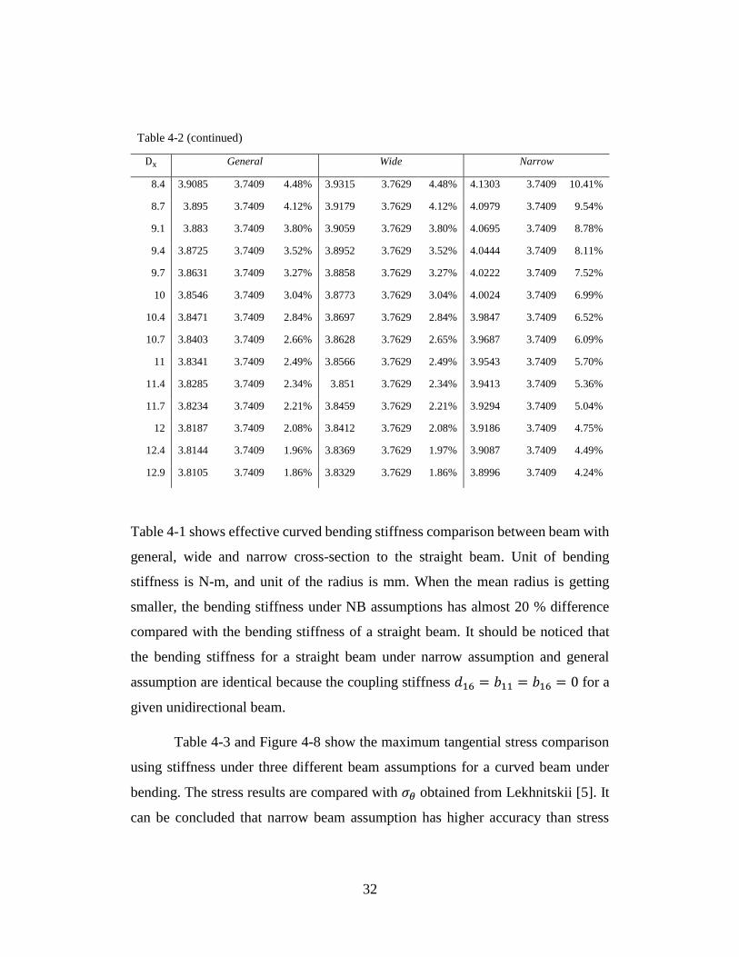
Table 4-1 shows effective curved bending stiffness comparison between beam with

general, wide and narrow cross-section to the straight beam. Unit of bending

stiffness is N-m, and unit of the radius is mm. When the mean radius is getting

smaller, the bending stiffness under NB assumptions has almost 20 % difference

compared with the bending stiffness of a straight beam. It should be noticed that

the bending stiffness for a straight beam under narrow assumption and general

assumption are identical because the coupling stiffness 𝑑16 = 𝑏11 = 𝑏16 = 0 for a

given unidirectional beam.

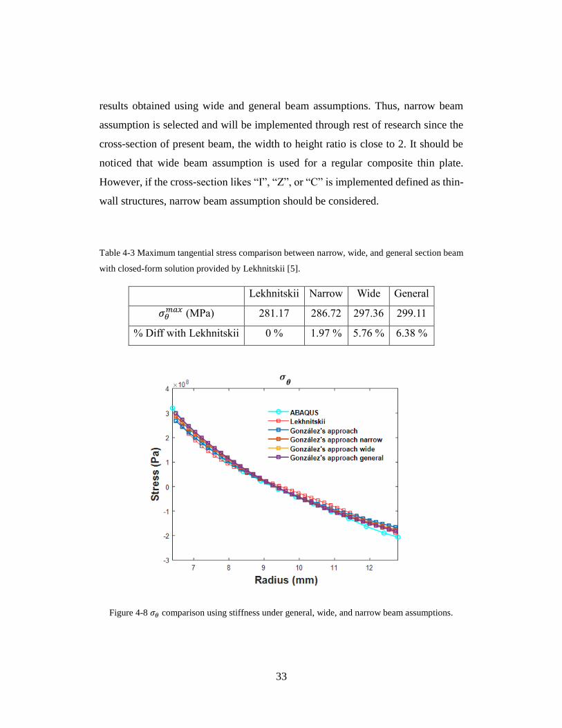
Table 4-3 and Figure 4-8 show the maximum tangential stress comparison

using stiffness under three different beam assumptions for a curved beam under

bending. The stress results are compared with 𝜎𝜃 obtained from Lekhnitskii [5]. It

can be concluded that narrow beam assumption has higher accuracy than stress

33

results obtained using wide and general beam assumptions. Thus, narrow beam

assumption is selected and will be implemented through rest of research since the

cross-section of present beam, the width to height ratio is close to 2. It should be

noticed that wide beam assumption is used for a regular composite thin plate.

However, if the cross-section likes “I”, “Z”, or “C” is implemented defined as thin-

wall structures, narrow beam assumption should be considered.

Table 4-3 Maximum tangential stress comparison between narrow, wide, and general section beam

with closed-form solution provided by Lekhnitskii [5].

Lekhnitskii Narrow Wide General

𝜎𝜃𝑚𝑎𝑥 (MPa) 281.17 286.72 297.36 299.11

% Diff with Lekhnitskii 0 % 1.97 % 5.76 % 6.38 %

Figure 4-8 𝜎𝜃 comparison using stiffness under general, wide, and narrow beam assumptions.

34

COMPOSITE CURVED BEAM WITH FIBER WAVINESS

Fiber waviness is a misalignment of the fibers in a ply. Fiber waviness

usually occurs due to residual stress which occurred from tooling or pressure from

the other layer. In addition, it can be caused by wrinkles or non-uniform

consolidation pressure. Fiber waviness results in stiffness and strength loss and acts

as a failure initiation in composite structures. This chapter describes the

development of analytical methodology for predicting in-plane and out-of-plane

fiber waviness in lamina or in laminate stage. The approach is based on definition

of fiber waviness shape. The averaging moduli is evaluated by considering the

shape of fiber waviness.

5-1 Effective Stiffness Properties for Straight In-Plane Lamina with Fiber

Waviness

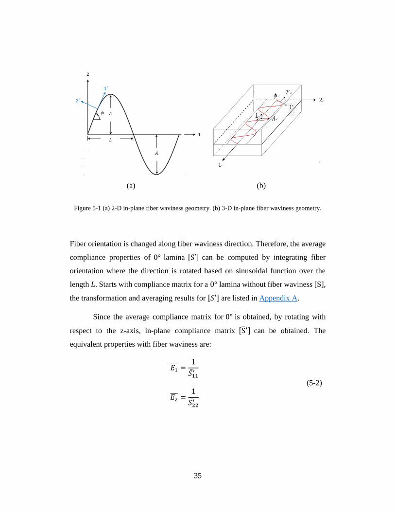
Fiber waviness can be expressed by a sinusoidal wave function in the 1-2

coordinate system as shown in Figure 5-1, where 𝑅 = 𝐴/𝐿 is a severity factor of

the curvature of fiber waviness, A is the amplitude of fiber waviness, and L is the

length of fiber waviness. As a result, the waviness angle 𝜙 can be introduced as

𝜙 = 𝑡𝑎𝑛−1 [𝜋𝑅 𝑐𝑜𝑠𝜋𝑥

𝐿]

(5-1)

35

Figure 5-1 (a) 2-D in-plane fiber waviness geometry. (b) 3-D in-plane fiber waviness geometry.

Fiber orientation is changed along fiber waviness direction. Therefore, the average

compliance properties of 0° lamina [S′] can be computed by integrating fiber

orientation where the direction is rotated based on sinusoidal function over the

length L. Starts with compliance matrix for a 0° lamina without fiber waviness [S],

the transformation and averaging results for [𝑆′] are listed in Appendix A.

Since the average compliance matrix for 0° is obtained, by rotating with

respect to the z-axis, in-plane compliance matrix [S′] can be obtained. The

equivalent properties with fiber waviness are:

𝐸1 =1

𝑆11′

𝐸2 =1

𝑆22′

(5-2)

(a) (b)

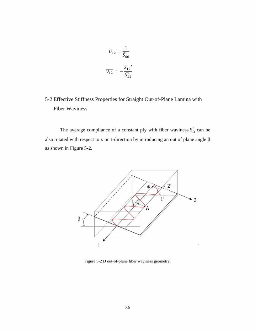
36

𝐺12 =1

𝑆66′

𝑣12 = −𝑆12′

𝑆11′

5-2 Effective Stiffness Properties for Straight Out-of-Plane Lamina with

Fiber Waviness

The average compliance of a constant ply with fiber waviness S𝑖𝑗′ can be

also rotated with respect to x or 1-direction by introducing an out of plane angle β

as shown in Figure 5-2.

Figure 5-2 D out-of-plane fiber waviness geometry.

37

After rotating with respect to the x-axis, the out-of-plane compliance matrix [S′′]

with average fiber waviness properties can be obtained using stress transformation

as shown below.

[S′′] = [Tε(−β)]𝑥[𝑆′][Tσ(β)]𝑥 (5-3)

where

[Tσ(𝛽)]x =

[ 1 0 00 𝑚2 𝑛2

0 𝑛2 𝑚2

0 0 02𝑚𝑛 0 0−2𝑚𝑛 0 0

0 −𝑚𝑛 𝑚𝑛0 0 00 0 0

𝑚2 − 𝑛2 0 00 𝑚 −𝑛0 𝑛 𝑚 ]

[Tε(β)]x =

[

1 0 00 𝑚2 𝑛2

0 𝑛2 𝑚2

0 0 0𝑚𝑛 0 0−𝑚𝑛 0 0

0 −2𝑚𝑛 2𝑚𝑛0 0 00 0 0

𝑚2 − 𝑛2 0 00 𝑚 −𝑛0 𝑛 𝑚 ]

(5-4)

and m = cos 𝛽 and n = sin 𝛽. The average stiffness properties can be expressed as

𝐸1 =1

S11′′

𝐸3 =1

S33′′

𝐺13 =1

S55′′

𝑣13 = −S13′′

S11′′

(5-5)

38

5-3 Effective Stiffness Properties of Composite Straight Laminate with In-

Plane and Out-of-Plane Fiber Waviness

In the previous section, the properties of a single layer with in-plane fiber

waviness is considered. To evaluate the laminate performance, CLT approach can

be used to obtain the average stiffness constant by considering of the summation

with the average compliance with fiber waviness [𝑆′] for a 0° unidirectional

laminate or [𝑆′] for multi-directional laminate for each layer.

[A] = ∑[𝑄′ 𝑥−𝑦]𝑘𝑡ℎ(𝑧𝑘 − 𝑧𝑘−1)

𝑛

𝑘=1

[B] =1

2∑[𝑄′𝑥−𝑦]𝑘𝑡ℎ

(𝑧𝑘2 − 𝑧𝑘−1

2 )

𝑛

𝑘=1

[D] =1

3∑[𝑄′𝑥−𝑦]𝑘𝑡ℎ

(𝑧𝑘3 − 𝑧𝑘−1

3 )

𝑛

𝑘=1

(5-6)

where

[𝑄′𝑥−𝑦]𝑘𝑡ℎ =[𝑆′]−1

(5-7)

Regarding with out-of-plane fiber waviness, the out-of-plane compliance

matrix can be computed by rotating in-plane properties 90° with respect to x-axis.

Thus, the stiffness tensor [𝑄] for each ply can be obtained by inversing compliance

matrix. Uniform out-of-plane fiber waviness is assumed. The amplitude of fiber

waviness, A, remains constant along thickness direction. The average compliance

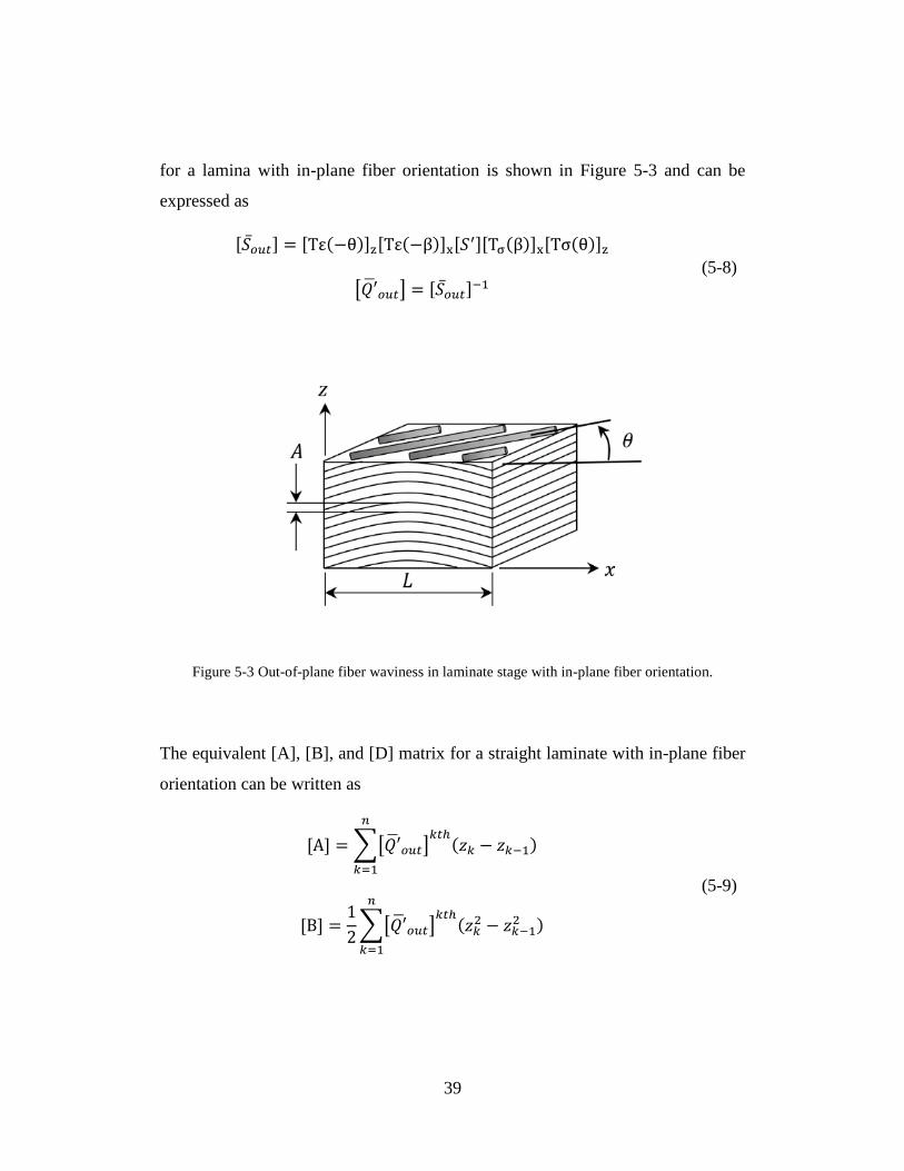
39

for a lamina with in-plane fiber orientation is shown in Figure 5-3 and can be

expressed as

[𝑆��𝑢𝑡] = [Tε(−θ)]z[Tε(−β)]x[𝑆′][Tσ(β)]x[Tσ(θ)]z

[𝑄′𝑜𝑢𝑡] = [𝑆��𝑢𝑡]−1

(5-8)

Figure 5-3 Out-of-plane fiber waviness in laminate stage with in-plane fiber orientation.

The equivalent [A], [B], and [D] matrix for a straight laminate with in-plane fiber

orientation can be written as

[A] = ∑[𝑄′𝑜𝑢𝑡]𝑘𝑡ℎ(𝑧𝑘 − 𝑧𝑘−1)

𝑛

𝑘=1

[B] =1

2∑[𝑄′𝑜𝑢𝑡]

𝑘𝑡ℎ(𝑧𝑘2 − 𝑧𝑘−1

2 )

𝑛

𝑘=1

(5-9)

40

D =1

3∑[𝑄′𝑜𝑢𝑡]

𝑘𝑡ℎ(𝑧𝑘3 − 𝑧𝑘−1

3 )

𝑛

𝑘=1

It should be noticed that [A], [B], and [D] matrix have dimensions 6 by 6 instead

of 3 by 3 because 3-D laminate behavior is considered.

5-4 Incremental Loading Scheme

The average stiffness properties alternate with the amplitude and length of fiber

waviness. During the preceding of increasing the strain, the fiber waviness

amplitude and fiber waviness length are changed, resulted in the effective moduli

reduces. For a given loading, stress can be transformed from x-y plane to 1-2

coordinate system and 1′-2′ (along fiber direction) coordinate system. Therefore,

the updated fiber waviness length and fiber length can be obtained. Based on

sinusoidal assumption, the updated amplitude can be computed. Since average

stiffness is functional of the amplitude and fiber waviness length, once the

amplitude and fiber waviness length are updated based on incremental strain, the

effective stiffness can be recalculated every iterations. The detail derivation is

shown in Appendix B and stated in Figure 5-4. It should be noted that the effective

stiffness result is very sensitive to the incremental strain. The total strain can be

accumulated based on the given little incremental strain. That incremental strain, if

tension is considered, it will lead to reduction of fiber waviness amplitude and

increment of fiber waviness length. If the given incremental strain is too limit,

insignificant changes for fiber waviness amplitude and length are observed.

Consequently, there is no significant stiffness reduction if the applied incremental

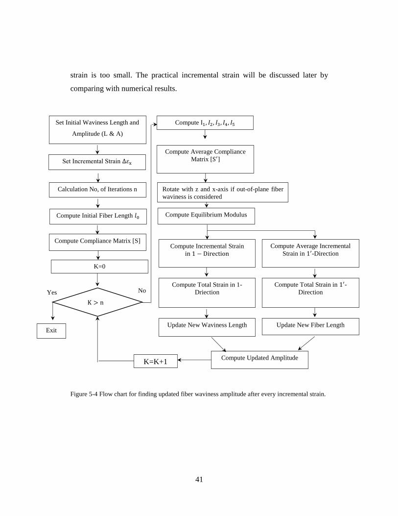
41

strain is too small. The practical incremental strain will be discussed later by

comparing with numerical results.

Figure 5-4 Flow chart for finding updated fiber waviness amplitude after every incremental strain.

Set Initial Waviness Length and

Amplitude (L & A)

Set Incremental Strain ∆𝜀x

Calculation No, of Iterations n

Compute Initial Fiber Length 𝑙0

Compute Compliance Matrix [S]

Compute I1, 𝐼2, 𝐼3, 𝐼4, 𝐼5

Compute Average Compliance

Matrix [S′]

Rotate with z and x-axis if out-of-plane fiber

waviness is considered

Compute Equilibrium Modulus

Compute Incremental Strain

in 1 − Direction

Compute Total Strain in 1-

Driection

Compute Average Incremental

Strain in 1′-Direction

Compute Total Strain in 1′-Direction

Update New Waviness Length Update New Fiber Length

Compute Updated Amplitude

K=0

K > n

K=K+1

No

Exit

Yes

42

5-5 Effective Stiffness Properties for Composite Curved Beam with In-

Plane and Out-of-Plane Fiber Waviness

Curved Lamina with in-plane fiber waviness is shown in Figure 5-5(a). The

average stiffness properties of curved lamina can be achieved by

replacing [��𝑥−𝑦]𝑘𝑡ℎto [𝑄′𝑥−𝑦]𝑘𝑡ℎ as shown in Eqs. (5-10). It should be noticed that

the uniform fiber waviness is assumed in this section. However, a graded fiber

waviness is often to be found and will be introduced for out-of-plane curved beam

model.

𝐴′c = Rm∑[𝑄′ 𝑥−𝑦]𝑘𝑡ℎln


𝑛

𝑘=1

𝐵′c = 𝑅𝑚∑[𝑄′ 𝑥−𝑦]𝑘𝑡ℎ[(𝑧𝑘 − 𝑧𝑘−1) − 𝑅𝑚 ln


]

𝑛

𝑘=1

𝐷′c = 𝑅𝑚∑[𝑄′ 𝑥−𝑦]𝑘𝑡ℎ[1

2(𝑧𝑘2 − 𝑧𝑘−1

2 ) − 𝑅𝑚(𝑧𝑘 − 𝑧𝑘−1) + 𝑅𝑚2 ln


]

𝑛

𝑘=1

(5-10)

Out-of-plane fiber waviness is characterized by raising and falling in the manner of

wavy layers. It will degrade the strength and fatigue performance of composite

structure. In general, non-uniform fiber waviness is observed along the curved

region instead of uniform fiber waviness distribution. Out-of-plane approach for

straight laminate can be applied to here by adjusting amplitude and length for fiber

waviness of each ply. The configuration of out-of-plane graded fiber waviness

along the curved region is shown in Figure 5-5(b), where 𝐿𝐴𝑒𝑛𝑑𝑡𝑜𝑝

and 𝐿𝐴𝑒𝑛𝑑𝑏𝑜𝑡 are the

location of plies where the zero amplitudes are observed on the configuration.

𝐿𝐴𝑚𝑎𝑥 is the ply location where the maximum amplitude of fiber waviness is

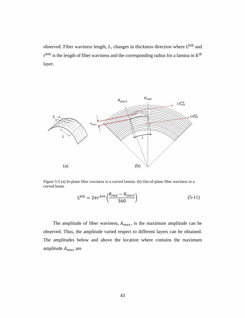
43

observed. Fiber waviness length, 𝐿, changes in thickness direction where Lkth and

rkth is the length of fiber waviness and the corresponding radius for a lamina in kth

layer.

Figure 5-5 (a) In-plane fiber waviness in a curved lamina. (b) Out-of-plane fiber waviness in a

curved beam.

Lkth = 2𝜋𝑟𝑘𝑡ℎ (𝜃𝑒𝑛𝑑 − 𝜃𝑠𝑡𝑎𝑟𝑡

360) (5-11)

The amplitude of fiber waviness, 𝐴𝑚𝑎𝑥 , is the maximum amplitude can be

observed. Thus, the amplitude varied respect to different layers can be obtained.

The amplitudes below and above the location where contains the maximum

amplitude 𝐴𝑚𝑎𝑥 are

(a) (b)

44

Alow =𝐴𝑚𝑎𝑥(𝑝𝑙𝑦

𝑡ℎ − 𝐿𝐴𝑒𝑛𝑑𝑏𝑜𝑡 )

𝐿𝐴𝑚𝑎𝑥 − 𝐿𝐴𝑒𝑛𝑑𝑏𝑜𝑡 for plyth = 𝐿𝐴𝑒𝑛𝑑

𝑏𝑜𝑡 𝑡𝑜 𝐿𝐴𝑚𝑎𝑥

Aupp = 𝐴𝑚𝑎𝑥 −𝐴𝑚𝑎𝑥(𝑝𝑙𝑦

𝑡ℎ − 𝐿𝐴𝑚𝑎𝑥 + 1)

𝐿𝐴𝑒𝑛𝑑𝑡𝑜𝑝 − 𝐿𝐴𝑚𝑎𝑥

for plyth

= 𝐿𝐴𝑚𝑎𝑥 𝑡𝑜 𝐿𝐴𝑒𝑛𝑑𝑡𝑜𝑝 − 1

(5-12)

where 𝑝𝑙𝑦𝑙𝑜𝑤𝑡ℎ = 𝐿𝐴𝑒𝑛𝑑

𝑏𝑜𝑡 ~ 𝐿𝐴𝑚𝑎𝑥 , and 𝑝𝑙𝑦𝑢𝑝𝑝𝑡ℎ = 𝐿𝐴𝑚𝑎𝑥 ~ 𝐿𝐴𝑒𝑛𝑑

𝑡𝑜𝑝− 1 . Thus, the

amplitude can be displaced as 𝐴𝑚𝑝𝑙𝑖𝑡𝑢𝑑𝑒 = [𝐴𝑙𝑜𝑤 , 𝐴𝑢𝑝𝑝] from bottom ply to the top ply

of entire curved beam.

Substituting Eqs. (5-12) into (5-8), the effective stiffness properties for a

composite curved beam with out-of-plane fiber waviness can be written as:

𝐴′c = Rm∑[𝑄′ 𝑜𝑢𝑡]𝑘𝑡ℎln


𝑛

𝑘=1

𝐵′c = 𝑅𝑚∑[𝑄′ 𝑜𝑢𝑡]𝑘𝑡ℎ[(𝑧𝑘 − 𝑧𝑘−1) − 𝑅𝑚 ln

𝑅 + 𝑧𝑘𝑅 + 𝑧𝑘−1

]

𝑛

𝑘=1

𝐷′c = 𝑅𝑚∑[𝑄′ 𝑜𝑢𝑡]𝑘𝑡ℎ[1

2(𝑧𝑘2 − 𝑧𝑘−1

2 ) − 𝑅𝑚(𝑧𝑘 − 𝑧𝑘−1) + 𝑅𝑚2 ln


]

𝑛

𝑘=1

(5-13)

5-6 Maximum Radial Stress Prediction

In Eqs. (4-24), 𝑄(1,1) can be replaced to [𝑄(1,1)𝑜𝑢𝑡]𝑘𝑡ℎ in order to obtain

equivalent stiffness in composite curved beam with fiber waviness. It should be noted

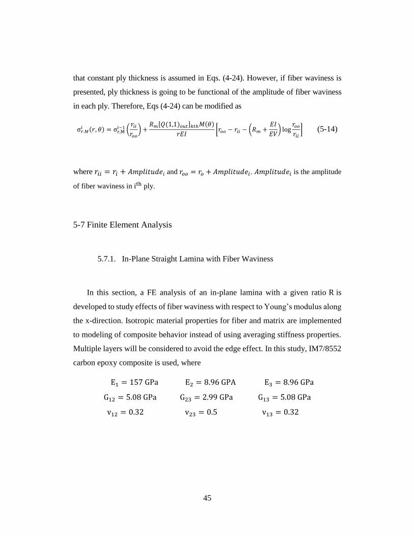
45

that constant ply thickness is assumed in Eqs. (4-24). However, if fiber waviness is

presented, ply thickness is going to be functional of the amplitude of fiber waviness

in each ply. Therefore, Eqs (4-24) can be modified as

σ𝑟.𝑀𝑖 (𝑟, 𝜃) = σr,M

i−1 (𝑟𝑖𝑖𝑟𝑜𝑜) +

𝑅𝑚[𝑄(1,1)𝑜𝑢𝑡]𝑘𝑡ℎ𝑀(𝜃)

𝑟𝐸𝐼[𝑟𝑜𝑜 − 𝑟𝑖𝑖 − (𝑅𝑚 +

𝐸𝐼

𝐸𝑉) log

𝑟𝑜𝑜𝑟𝑖𝑖] (5-14)

where 𝑟𝑖𝑖 = 𝑟𝑖 + 𝐴𝑚𝑝𝑙𝑖𝑡𝑢𝑑𝑒𝑖 and 𝑟𝑜𝑜 = 𝑟𝑜 + 𝐴𝑚𝑝𝑙𝑖𝑡𝑢𝑑𝑒𝑖. 𝐴𝑚𝑝𝑙𝑖𝑡𝑢𝑑𝑒𝑖 is the amplitude

of fiber waviness in ith ply.

5-7 Finite Element Analysis

5.7.1. In-Plane Straight Lamina with Fiber Waviness

In this section, a FE analysis of an in-plane lamina with a given ratio R is

developed to study effects of fiber waviness with respect to Young’s modulus along

the x-direction. Isotropic material properties for fiber and matrix are implemented

to modeling of composite behavior instead of using averaging stiffness properties.

Multiple layers will be considered to avoid the edge effect. In this study, IM7/8552

carbon epoxy composite is used, where

E1 = 157 GPa E2 = 8.96 GPA E3 = 8.96 GPa

G12 = 5.08 GPa G23 = 2.99 GPa G13 = 5.08 GPa

v12 = 0.32 v23 = 0.5 v13 = 0.32

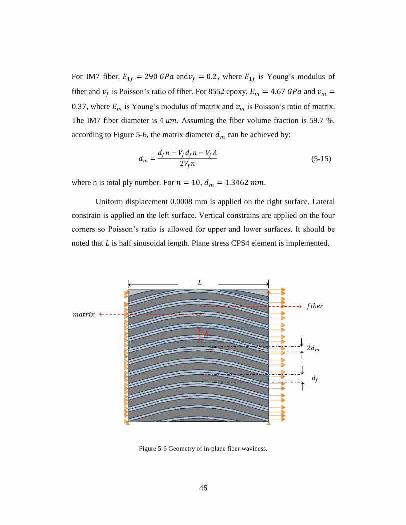
46

For IM7 fiber, 𝐸1𝑓 = 290 𝐺𝑃𝑎 and𝑣𝑓 = 0.2, where 𝐸1𝑓 is Young’s modulus of

fiber and 𝑣𝑓 is Poisson’s ratio of fiber. For 8552 epoxy, 𝐸𝑚 = 4.67 𝐺𝑃𝑎 and 𝑣𝑚 =

0.37, where 𝐸𝑚 is Young’s modulus of matrix and 𝑣𝑚 is Poisson’s ratio of matrix.

The IM7 fiber diameter is 4 𝜇𝑚. Assuming the fiber volume fraction is 59.7 %,

according to Figure 5-6, the matrix diameter 𝑑𝑚 can be achieved by:

𝑑𝑚 =𝑑𝑓𝑛 − 𝑉𝑓𝑑𝑓𝑛 − 𝑉𝑓𝐴

2𝑉𝑓𝑛 (5-15)

where n is total ply number. For 𝑛 = 10, 𝑑𝑚 = 1.3462 𝑚𝑚.

Uniform displacement 0.0008 mm is applied on the right surface. Lateral

constrain is applied on the left surface. Vertical constrains are applied on the four

corners so Poisson’s ratio is allowed for upper and lower surfaces. It should be

noted that 𝐿 is half sinusoidal length. Plane stress CPS4 element is implemented.

Figure 5-6 Geometry of in-plane fiber waviness.

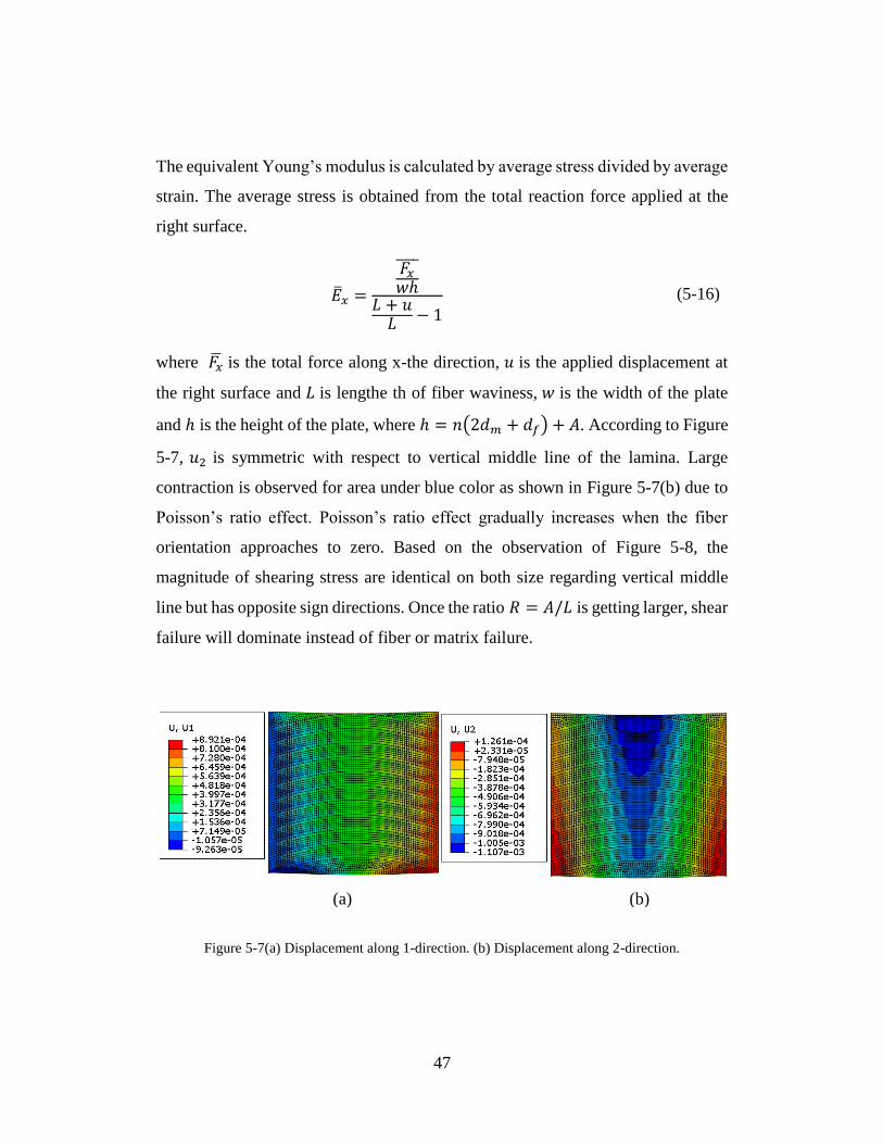
47

The equivalent Young’s modulus is calculated by average stress divided by average

strain. The average stress is obtained from the total reaction force applied at the

right surface.

��𝑥 =

𝐹𝑥𝑤ℎ

𝐿 + 𝑢𝐿 − 1

(5-16)

where 𝐹�� is the total force along x-the direction, 𝑢 is the applied displacement at

the right surface and 𝐿 is lengthe th of fiber waviness, 𝑤 is the width of the plate

and ℎ is the height of the plate, where ℎ = 𝑛(2𝑑𝑚 + 𝑑𝑓) + 𝐴. According to Figure

5-7, 𝑢2 is symmetric with respect to vertical middle line of the lamina. Large

contraction is observed for area under blue color as shown in Figure 5-7(b) due to

Poisson’s ratio effect. Poisson’s ratio effect gradually increases when the fiber

orientation approaches to zero. Based on the observation of Figure 5-8, the

magnitude of shearing stress are identical on both size regarding vertical middle

line but has opposite sign directions. Once the ratio 𝑅 = 𝐴/𝐿 is getting larger, shear

failure will dominate instead of fiber or matrix failure.

Figure 5-7(a) Displacement along 1-direction. (b) Displacement along 2-direction.

(a) (b)

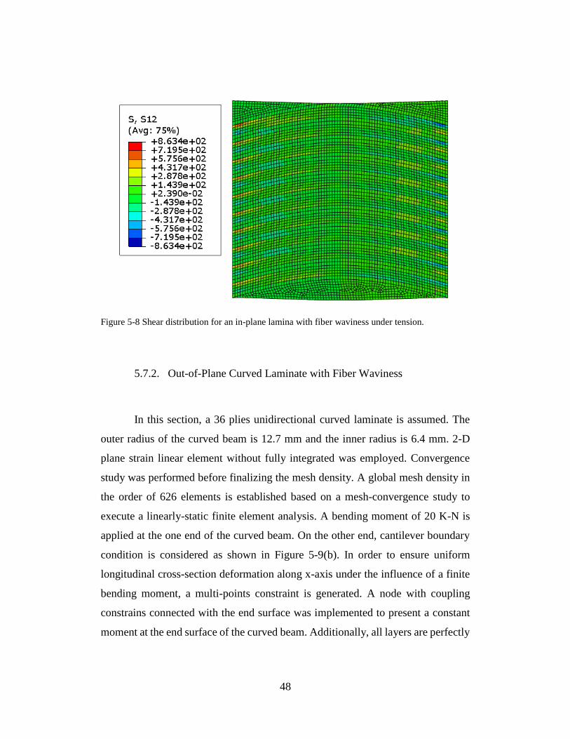
48

Figure 5-8 Shear distribution for an in-plane lamina with fiber waviness under tension.

5.7.2. Out-of-Plane Curved Laminate with Fiber Waviness

In this section, a 36 plies unidirectional curved laminate is assumed. The

outer radius of the curved beam is 12.7 mm and the inner radius is 6.4 mm. 2-D

plane strain linear element without fully integrated was employed. Convergence

study was performed before finalizing the mesh density. A global mesh density in

the order of 626 elements is established based on a mesh-convergence study to

execute a linearly-static finite element analysis. A bending moment of 20 K-N is

applied at the one end of the curved beam. On the other end, cantilever boundary

condition is considered as shown in Figure 5-9(b). In order to ensure uniform

longitudinal cross-section deformation along x-axis under the influence of a finite

bending moment, a multi-points constraint is generated. A node with coupling

constrains connected with the end surface was implemented to present a constant

moment at the end surface of the curved beam. Additionally, all layers are perfectly

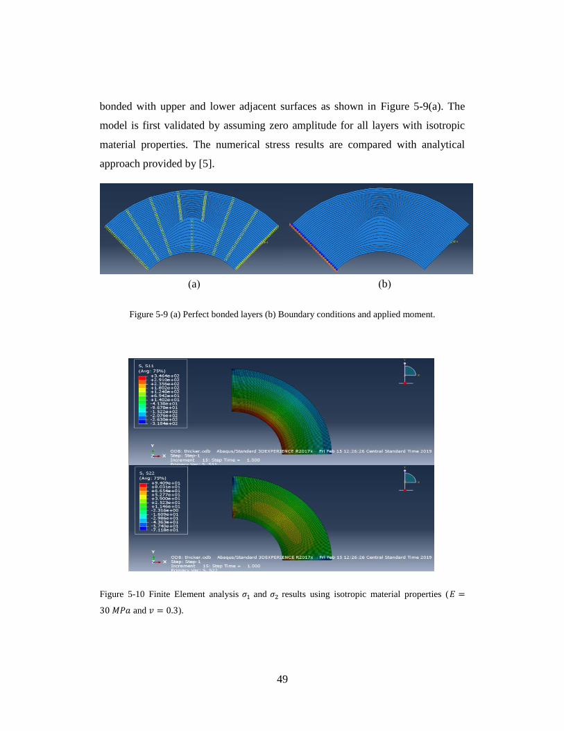
49

bonded with upper and lower adjacent surfaces as shown in Figure 5-9(a). The

model is first validated by assuming zero amplitude for all layers with isotropic

material properties. The numerical stress results are compared with analytical

approach provided by [5].

Figure 5-9 (a) Perfect bonded layers (b) Boundary conditions and applied moment.

Figure 5-10 Finite Element analysis 𝜎1 and 𝜎2 results using isotropic material properties (𝐸 =

30 𝑀𝑃𝑎 and 𝑣 = 0.3).

(a) (b)

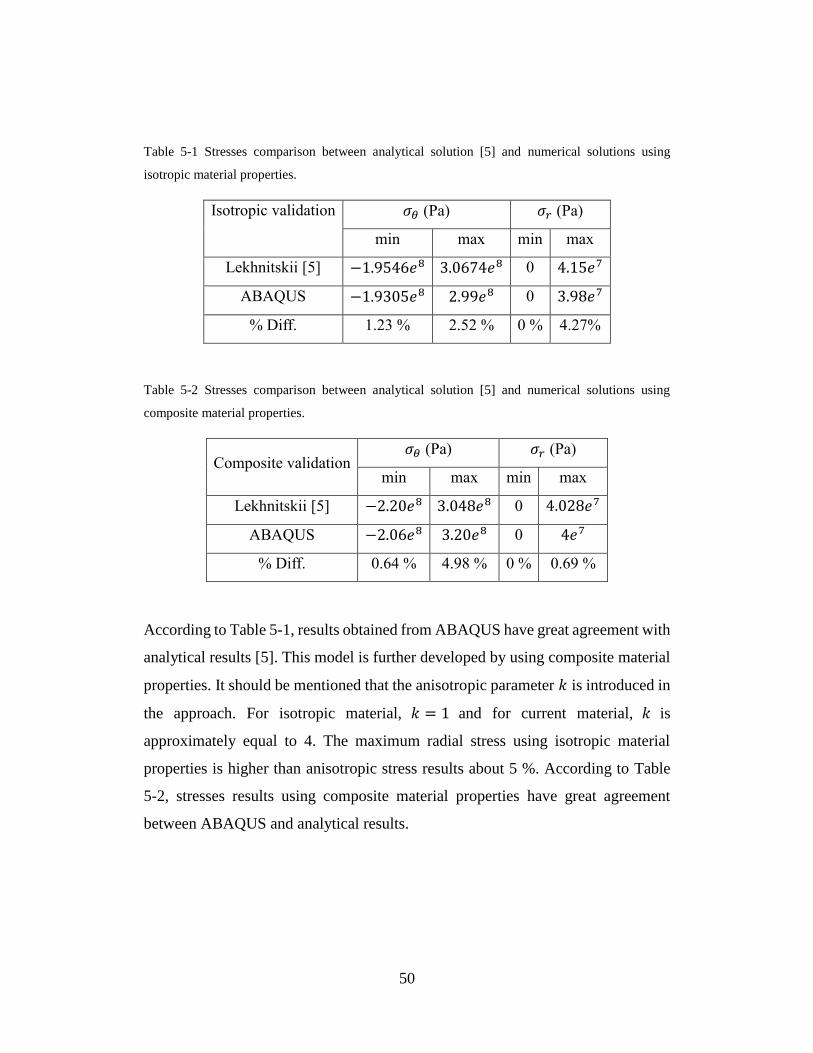
50

Table 5-1 Stresses comparison between analytical solution [5] and numerical solutions using

isotropic material properties.

Isotropic validation 𝜎𝜃 (Pa) 𝜎𝑟 (Pa)

min max min max

Lekhnitskii [5] −1.9546𝑒8 3.0674𝑒8 0 4.15𝑒7

ABAQUS −1.9305𝑒8 2.99𝑒8 0 3.98𝑒7

% Diff. 1.23 % 2.52 % 0 % 4.27%

Table 5-2 Stresses comparison between analytical solution [5] and numerical solutions using

composite material properties.

Composite validation 𝜎𝜃 (Pa) 𝜎𝑟 (Pa)

min max min max

Lekhnitskii [5] −2.20𝑒8 3.048𝑒8 0 4.028𝑒7

ABAQUS −2.06𝑒8 3.20𝑒8 0 4𝑒7

% Diff. 0.64 % 4.98 % 0 % 0.69 %

According to Table 5-1, results obtained from ABAQUS have great agreement with

analytical results [5]. This model is further developed by using composite material

properties. It should be mentioned that the anisotropic parameter 𝑘 is introduced in

the approach. For isotropic material, 𝑘 = 1 and for current material, 𝑘 is

approximately equal to 4. The maximum radial stress using isotropic material

properties is higher than anisotropic stress results about 5 %. According to Table

5-2, stresses results using composite material properties have great agreement

between ABAQUS and analytical results.

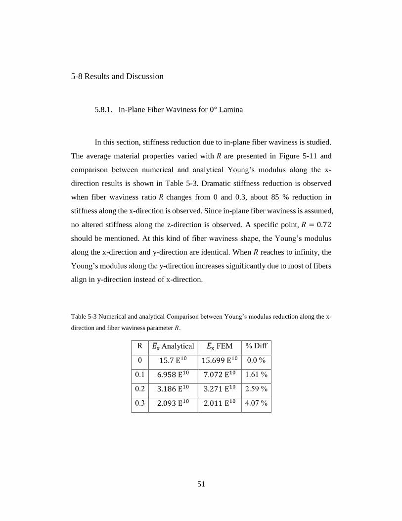
51

5-8 Results and Discussion

5.8.1. In-Plane Fiber Waviness for 0° Lamina

In this section, stiffness reduction due to in-plane fiber waviness is studied.

The average material properties varied with 𝑅 are presented in Figure 5-11 and

comparison between numerical and analytical Young’s modulus along the x-

direction results is shown in Table 5-3. Dramatic stiffness reduction is observed

when fiber waviness ratio 𝑅 changes from 0 and 0.3, about 85 % reduction in

stiffness along the x-direction is observed. Since in-plane fiber waviness is assumed,

no altered stiffness along the z-direction is observed. A specific point, 𝑅 = 0.72

should be mentioned. At this kind of fiber waviness shape, the Young’s modulus

along the x-direction and y-direction are identical. When 𝑅 reaches to infinity, the

Young’s modulus along the y-direction increases significantly due to most of fibers

align in y-direction instead of x-direction.

Table 5-3 Numerical and analytical Comparison between Young’s modulus reduction along the x-

direction and fiber waviness parameter 𝑅.

R ��x Analytical ��x FEM % Diff

0 15.7 E10 15.699 E10 0.0 %

0.1 6.958 E10 7.072 E10 1.61 %

0.2 3.186 E10 3.271 E10 2.59 %

0.3 2.093 E10 2.011 E10 4.07 %

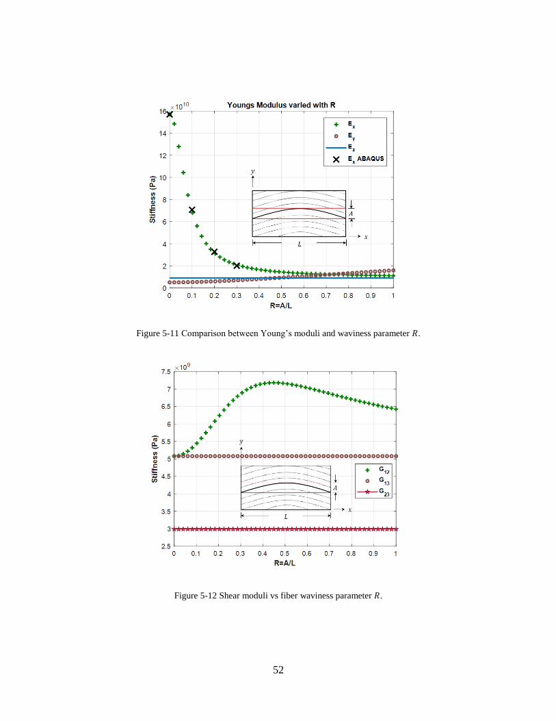
52

Figure 5-11 Comparison between Young’s moduli and waviness parameter 𝑅.

Figure 5-12 Shear moduli vs fiber waviness parameter 𝑅.

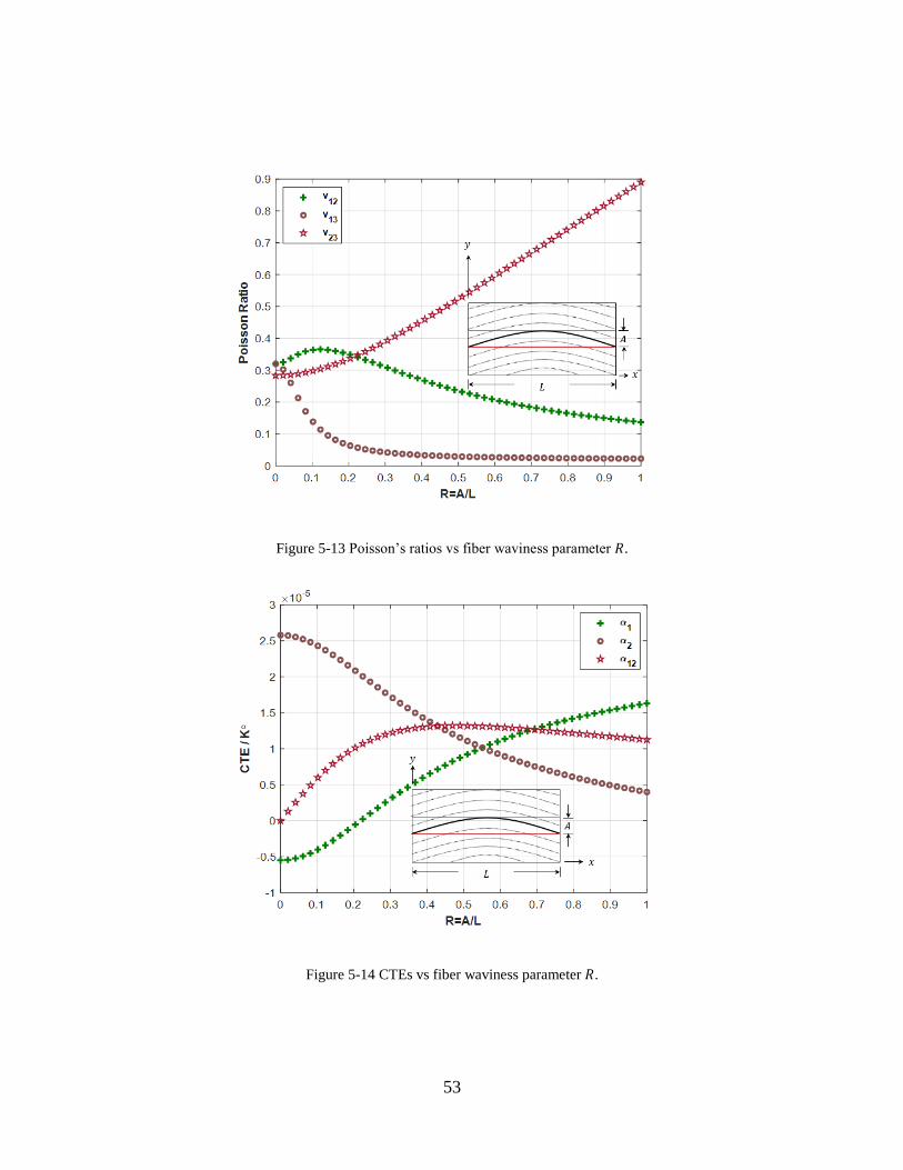
53

Figure 5-13 Poisson’s ratios vs fiber waviness parameter 𝑅.

Figure 5-14 CTEs vs fiber waviness parameter 𝑅.

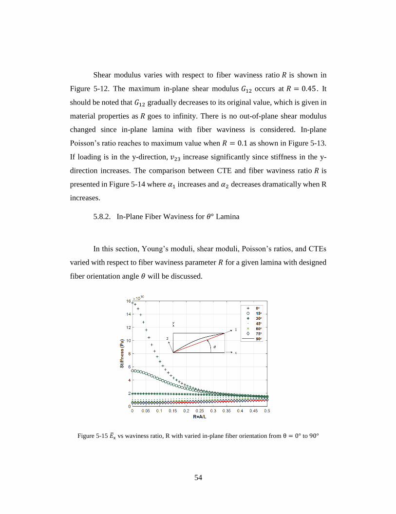
54

Shear modulus varies with respect to fiber waviness ratio 𝑅 is shown in

Figure 5-12. The maximum in-plane shear modulus 𝐺12 occurs at 𝑅 = 0.45 . It

should be noted that 𝐺12 gradually decreases to its original value, which is given in

material properties as 𝑅 goes to infinity. There is no out-of-plane shear modulus

changed since in-plane lamina with fiber waviness is considered. In-plane

Poisson’s ratio reaches to maximum value when 𝑅 = 0.1 as shown in Figure 5-13.

If loading is in the y-direction, 𝑣23 increase significantly since stiffness in the y-

direction increases. The comparison between CTE and fiber waviness ratio 𝑅 is

presented in Figure 5-14 where 𝛼1 increases and 𝛼2 decreases dramatically when R

increases.

5.8.2. In-Plane Fiber Waviness for 𝜃° Lamina

In this section, Young’s moduli, shear moduli, Poisson’s ratios, and CTEs

varied with respect to fiber waviness parameter 𝑅 for a given lamina with designed

fiber orientation angle 𝜃 will be discussed.

Figure 5-15 ��x vs waviness ratio, R with varied in-plane fiber orientation from θ = 0° to 90°

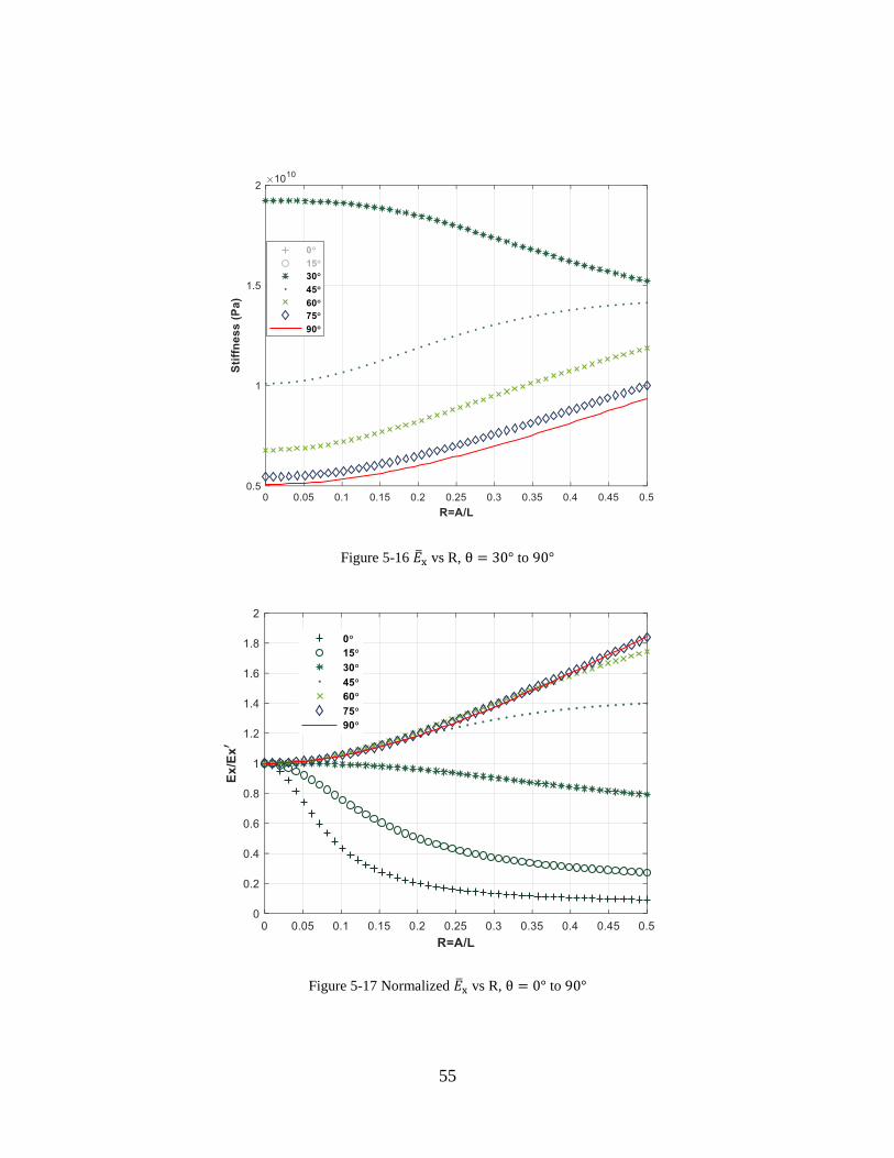
55

Figure 5-16 ��x vs R, θ = 30° to 90°

Figure 5-17 Normalized ��x vs R, θ = 0° to 90°

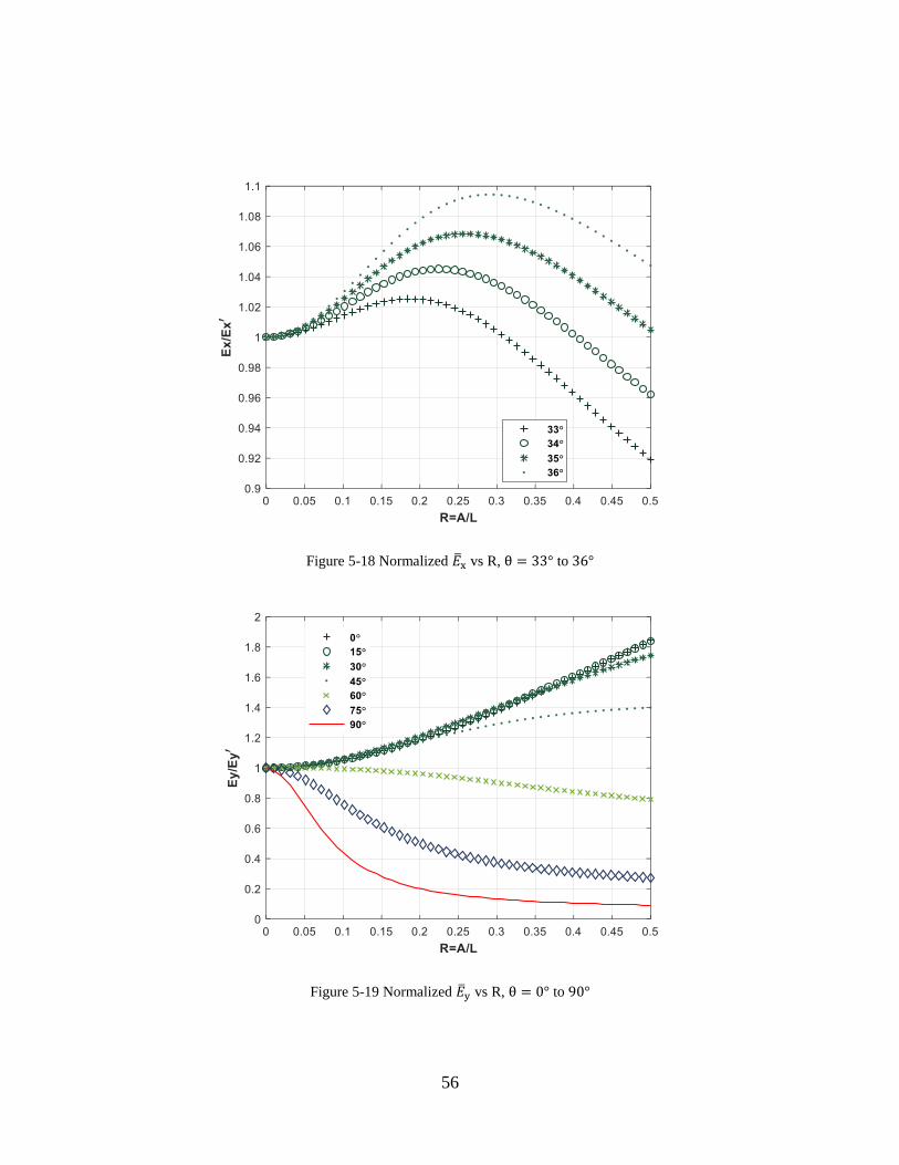
56

Figure 5-18 Normalized ��x vs R, θ = 33° to 36°

Figure 5-19 Normalized ��y vs R, θ = 0° to 90°

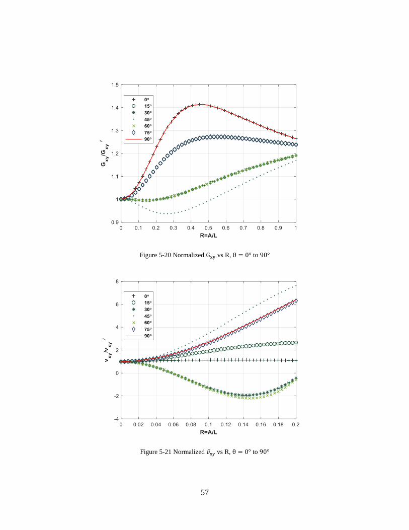
57

Figure 5-20 Normalized Gxy vs R, θ = 0° to 90°

Figure 5-21 Normalized ��xy vs R, θ = 0° to 90°

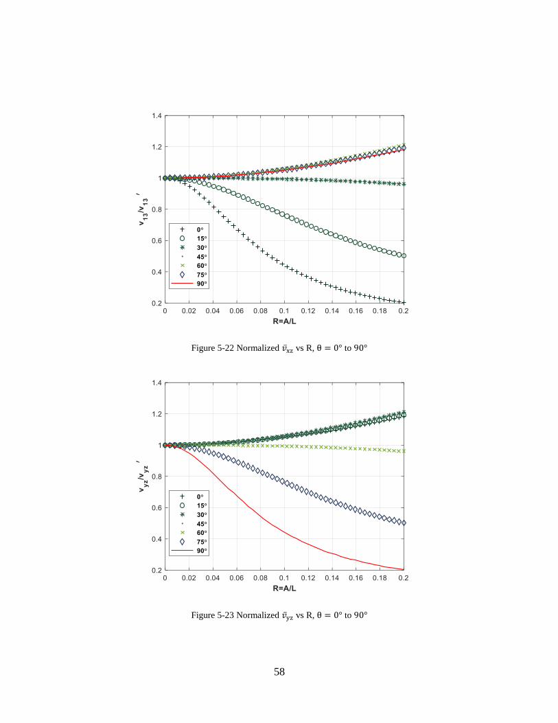
58

Figure 5-22 Normalized ��xz vs R, θ = 0° to 90°

Figure 5-23 Normalized ��yz vs R, θ = 0° to 90°

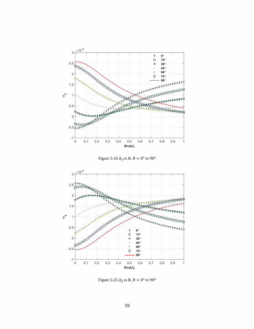
59

Figure 5-24 ��𝑥vs R, θ = 0° to 90°

Figure 5-25 ��𝑦vs R, θ = 0° to 90°

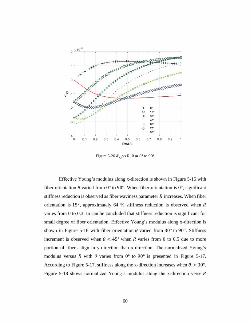
60

Figure 5-26 ��𝑥𝑦vs R, θ = 0° to 90°

Effective Young’s modulus along x-direction is shown in Figure 5-15 with

fiber orientation 𝜃 varied from 0° to 90°. When fiber orientation is 0°, significant

stiffness reduction is observed as fiber waviness parameter 𝑅 increases. When fiber

orientation is 15°, approximately 64 % stiffness reduction is observed when 𝑅

varies from 0 to 0.3. In can be concluded that stiffness reduction is significant for

small degree of fiber orientation. Effective Young’s modulus along x-direction is

shown in Figure 5-16 with fiber orientation 𝜃 varied from 30° to 90°. Stiffness

increment is observed when 𝜃 < 45° when 𝑅 varies from 0 to 0.5 due to more

portion of fibers align in y-direction than x-direction. The normalized Young’s

modulus versus 𝑅 with 𝜃 varies from 0° to 90° is presented in Figure 5-17.

According to Figure 5-17, stiffness along the x-direction increases when 𝜃 > 30°.

Figure 5-18 shows normalized Young’s modulus along the x-direction verse 𝑅

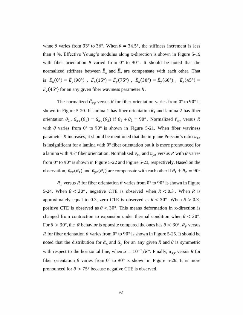
61

whne 𝜃 varies from 33° to 36°. When 𝜃 = 34.5°, the stiffness increment is less

than 4 %. Effective Young’s modulus along x-direction is shown in Figure 5-19

with fiber orientation 𝜃 varied from 0° to 90° . It should be noted that the

normalized stiffness between ��x and ��y are compensate with each other. That

is ��x(0°) = ��y(90°) , ��x(15°) = ��y(75°) , ��x(30°) = ��y(60°) , ��x(45°) =

��y(45°) for an any given fiber waviness parameter 𝑅.

The normalized ��𝑥𝑦 versus 𝑅 for fiber orientation varies from 0° to 90° is

shown in Figure 5-20. If lamina 1 has fiber orientation 𝜃1 and lamina 2 has fiber

orientation 𝜃2 , ��𝑥𝑦(𝜃1) = ��𝑥𝑦(𝜃2) if 𝜃1 + 𝜃2 = 90° . Normalized ��𝑥𝑦 versus 𝑅

with 𝜃 varies from 0° to 90° is shown in Figure 5-21. When fiber waviness

parameter 𝑅 increases, it should be mentioned that the in-plane Poisson’s ratio 𝑣12

is insignificant for a lamina with 0° fiber orientation but it is more pronounced for

a lamina with 45° fiber orientation. Normalized ��𝑥𝑧 and ��𝑦𝑧 versus 𝑅 with 𝜃 varies

from 0° to 90° is shown in Figure 5-22 and Figure 5-23, respectively. Based on the

observation, ��𝑥𝑧(𝜃1) and ��𝑦𝑧(𝜃2) are compensate with each other if 𝜃1 + 𝜃2 = 90°.

��𝑥 versus 𝑅 for fiber orientation 𝜃 varies from 0° to 90° is shown in Figure

5-24. When 𝜃 < 30° , negative CTE is observed when 𝑅 < 0.3 . When 𝑅 is

approximately equal to 0.3, zero CTE is observed as 𝜃 < 30°. When 𝑅 > 0.3,

positive CTE is observed as 𝜃 < 30°. This means deformation in x-direction is

changed from contraction to expansion under thermal condition when 𝜃 < 30°.

For 𝜃 > 30°, the �� behavior is opposite compared the ones has 𝜃 < 30°. ��y versus

𝑅 for fiber orientation 𝜃 varies from 0° to 90° is shown in Figure 5-25. It should be

noted that the distribution for ��x and ��y for an any given 𝑅 and 𝜃 is symmetric

with respect to the horizontal line, when 𝛼 = 10−5/𝐾°. Finally, ��𝑥𝑦 versus 𝑅 for

fiber orientation 𝜃 varies from 0° to 90° is shown in Figure 5-26. It is more

pronounced for 𝜃 > 75° because negative CTE is observed.

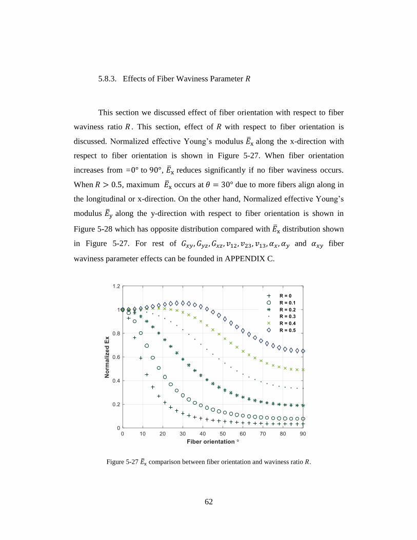
62

5.8.3. Effects of Fiber Waviness Parameter 𝑅

This section we discussed effect of fiber orientation with respect to fiber

waviness ratio 𝑅 . This section, effect of 𝑅 with respect to fiber orientation is

discussed. Normalized effective Young’s modulus ��x along the x-direction with

respect to fiber orientation is shown in Figure 5-27. When fiber orientation

increases from =0° to 90°, ��x reduces significantly if no fiber waviness occurs.

When 𝑅 > 0.5, maximum ��x occurs at 𝜃 = 30° due to more fibers align along in

the longitudinal or x-direction. On the other hand, Normalized effective Young’s

modulus ��y along the y-direction with respect to fiber orientation is shown in

Figure 5-28 which has opposite distribution compared with ��x distribution shown

in Figure 5-27. For rest of 𝐺𝑥𝑦, 𝐺𝑦𝑧 , 𝐺𝑥𝑧 , 𝑣12, 𝑣23, 𝑣13, 𝛼𝑥 , 𝛼𝑦 and 𝛼𝑥𝑦 fiber

waviness parameter effects can be founded in APPENDIX C.

Figure 5-27 ��x comparison between fiber orientation and waviness ratio 𝑅.

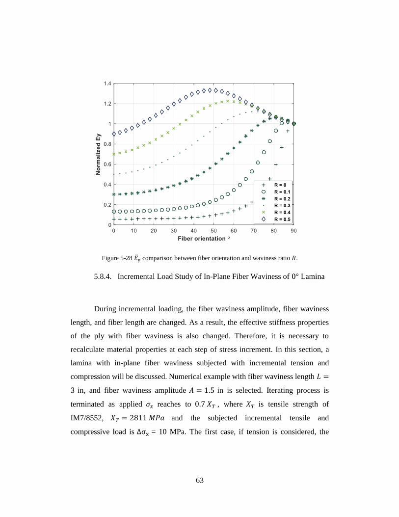
63

Figure 5-28 ��y comparison between fiber orientation and waviness ratio 𝑅.

5.8.4. Incremental Load Study of In-Plane Fiber Waviness of 0° Lamina

During incremental loading, the fiber waviness amplitude, fiber waviness

length, and fiber length are changed. As a result, the effective stiffness properties

of the ply with fiber waviness is also changed. Therefore, it is necessary to

recalculate material properties at each step of stress increment. In this section, a

lamina with in-plane fiber waviness subjected with incremental tension and

compression will be discussed. Numerical example with fiber waviness length 𝐿 =

3 in, and fiber waviness amplitude 𝐴 = 1.5 in is selected. Iterating process is

terminated as applied 𝜎𝑥 reaches to 0.7 𝑋𝑇 , where 𝑋𝑇 is tensile strength of

IM7/8552, 𝑋𝑇 = 2811 𝑀𝑃𝑎 and the subjected incremental tensile and

compressive load is ∆σx = 10 MPa. The first case, if tension is considered, the

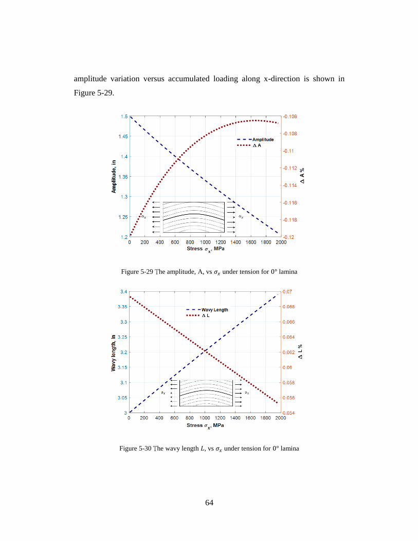
64

amplitude variation versus accumulated loading along x-direction is shown in

Figure 5-29.

Figure 5-29 The amplitude, A, vs 𝜎𝑥 under tension for 0° lamina

Figure 5-30 The wavy length 𝐿, vs 𝜎𝑥 under tension for 0° lamina

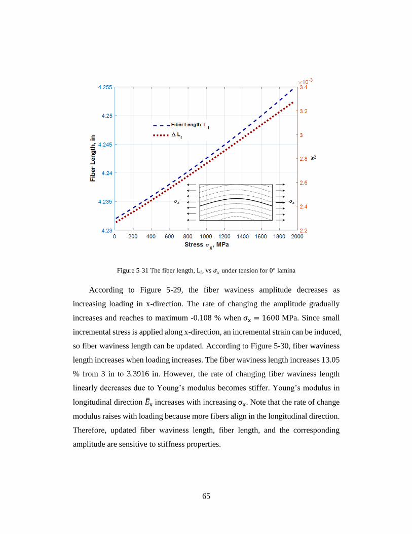
65

Figure 5-31 The fiber length, Lf, vs 𝜎𝑥 under tension for 0° lamina

According to Figure 5-29, the fiber waviness amplitude decreases as

increasing loading in x-direction. The rate of changing the amplitude gradually

increases and reaches to maximum -0.108 % when σx = 1600 MPa. Since small

incremental stress is applied along x-direction, an incremental strain can be induced,

so fiber waviness length can be updated. According to Figure 5-30, fiber waviness

length increases when loading increases. The fiber waviness length increases 13.05

% from 3 in to 3.3916 in. However, the rate of changing fiber waviness length

linearly decreases due to Young’s modulus becomes stiffer. Young’s modulus in

longitudinal direction ��x increases with increasing σx. Note that the rate of change

modulus raises with loading because more fibers align in the longitudinal direction.

Therefore, updated fiber waviness length, fiber length, and the corresponding

amplitude are sensitive to stiffness properties.

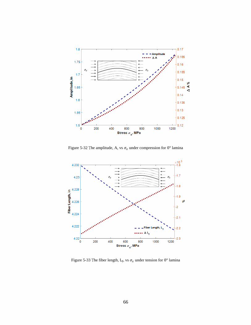
66

Figure 5-32 The amplitude, A, vs 𝜎𝑥 under compression for 0° lamina

Figure 5-33 The fiber length, Lf, vs 𝜎𝑥 under tension for 0° lamina

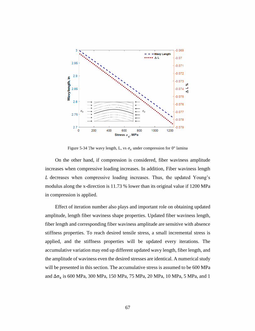
67

Figure 5-34 The wavy length, L, vs 𝜎𝑥 under compression for 0° lamina

On the other hand, if compression is considered, fiber waviness amplitude

increases when compressive loading increases. In addition, Fiber waviness length

𝐿 decreases when compressive loading increases. Thus, the updated Young’s

modulus along the x-direction is 11.73 % lower than its original value if 1200 MPa

in compression is applied.

Effect of iteration number also plays and important role on obtaining updated

amplitude, length fiber waviness shape properties. Updated fiber waviness length,

fiber length and corresponding fiber waviness amplitude are sensitive with absence

stiffness properties. To reach desired tensile stress, a small incremental stress is

applied, and the stiffness properties will be updated every iterations. The

accumulative variation may end up different updated wavy length, fiber length, and

the amplitude of waviness even the desired stresses are identical. A numerical study

will be presented in this section. The accumulative stress is assumed to be 600 MPa

and Δσx is 600 MPa, 300 MPa, 150 MPa, 75 MPa, 20 MPa, 10 MPa, 5 MPa, and 1

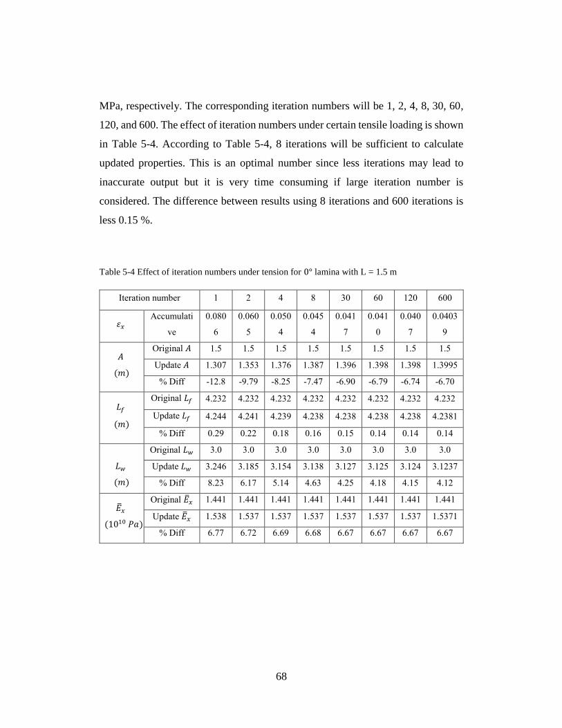
68

MPa, respectively. The corresponding iteration numbers will be 1, 2, 4, 8, 30, 60,

120, and 600. The effect of iteration numbers under certain tensile loading is shown

in Table 5-4. According to Table 5-4, 8 iterations will be sufficient to calculate

updated properties. This is an optimal number since less iterations may lead to

inaccurate output but it is very time consuming if large iteration number is

considered. The difference between results using 8 iterations and 600 iterations is

less 0.15 %.

Table 5-4 Effect of iteration numbers under tension for 0° lamina with L = 1.5 m

Iteration number 1 2 4 8 30 60 120 600

𝜀𝑥 Accumulati

ve

0.080

6

0.060

5

0.050

4

0.045

4

0.041

7

0.041

0

0.040

7

0.0403

9

𝐴

(𝑚)

Original 𝐴 1.5 1.5 1.5 1.5 1.5 1.5 1.5 1.5

Update 𝐴 1.307 1.353 1.376 1.387 1.396 1.398 1.398 1.3995

% Diff -12.8 -9.79 -8.25 -7.47 -6.90 -6.79 -6.74 -6.70

𝐿𝑓

(𝑚)

Original 𝐿𝑓 4.232 4.232 4.232 4.232 4.232 4.232 4.232 4.232

Update 𝐿𝑓 4.244 4.241 4.239 4.238 4.238 4.238 4.238 4.2381

% Diff 0.29 0.22 0.18 0.16 0.15 0.14 0.14 0.14

𝐿𝑤

(𝑚)

Original 𝐿𝑤 3.0 3.0 3.0 3.0 3.0 3.0 3.0 3.0

Update 𝐿𝑤 3.246 3.185 3.154 3.138 3.127 3.125 3.124 3.1237

% Diff 8.23 6.17 5.14 4.63 4.25 4.18 4.15 4.12

��𝑥

(1010 𝑃𝑎)

Original ��𝑥 1.441 1.441 1.441 1.441 1.441 1.441 1.441 1.441

Update ��𝑥 1.538 1.537 1.537 1.537 1.537 1.537 1.537 1.5371

% Diff 6.77 6.72 6.69 6.68 6.67 6.67 6.67 6.67

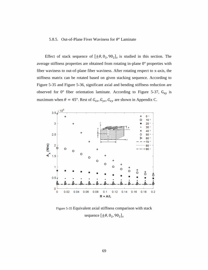
69

5.8.5. Out-of-Plane Fiver Waviness for 𝜃° Laminate

Effect of stack sequence of [±𝜃, 02, 902]𝑠 is studied in this section. The

average stiffness properties are obtained from rotating in-plane 0° properties with

fiber waviness to out-of-plane fiber waviness. After rotating respect to x-axis, the

stiffness matrix can be rotated based on given stacking sequence. According to

Figure 5-35 and Figure 5-36, significant axial and bending stiffness reduction are

observed for 0° fiber orientation laminate. According to Figure 5-37, Gxy is

maximum when 𝜃 = 45°. Rest of 𝐺𝑥𝑧 , 𝐺𝑦𝑧 , 𝐺𝑥𝑦 are shown in Appendix C.

Figure 5-35 Equivalent axial stiffness comparison with stack

sequence [±𝜃, 02, 902]𝑠

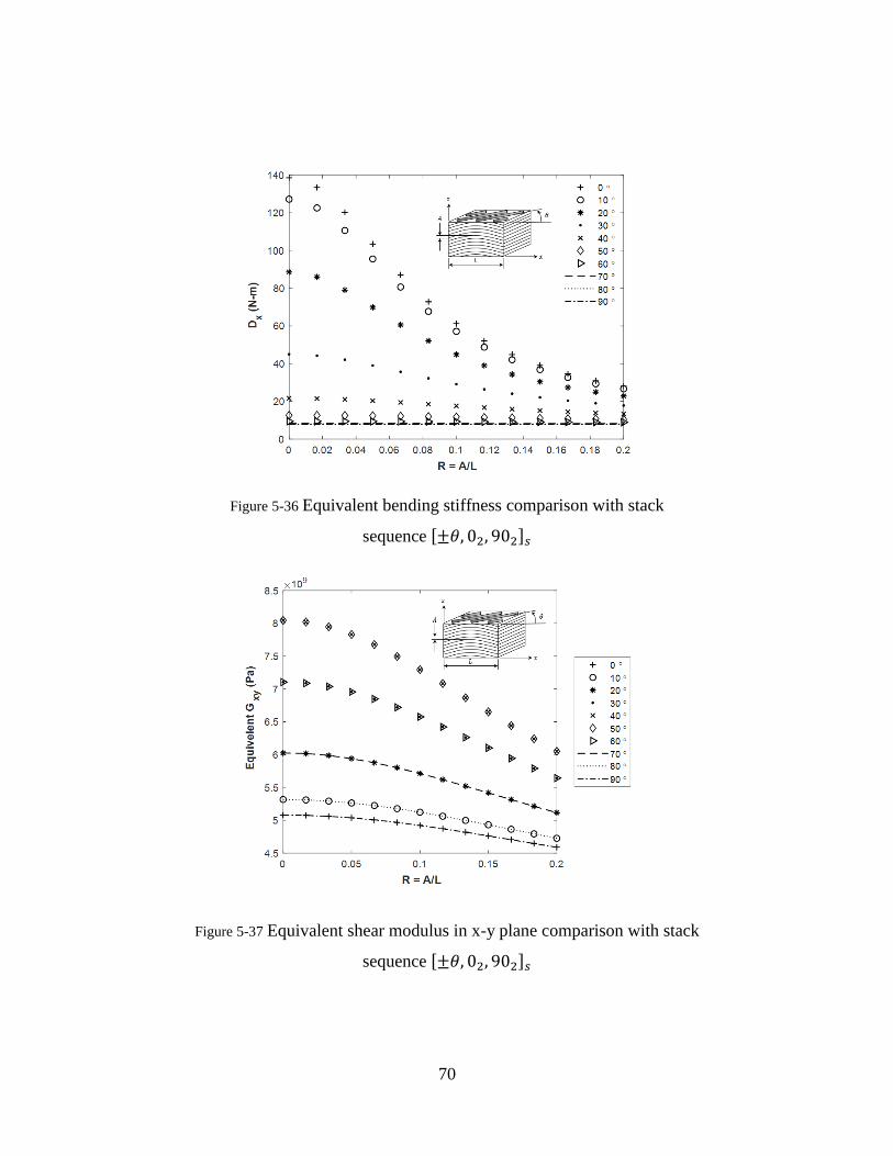
70

Figure 5-36 Equivalent bending stiffness comparison with stack


Figure 5-37 Equivalent shear modulus in x-y plane comparison with stack


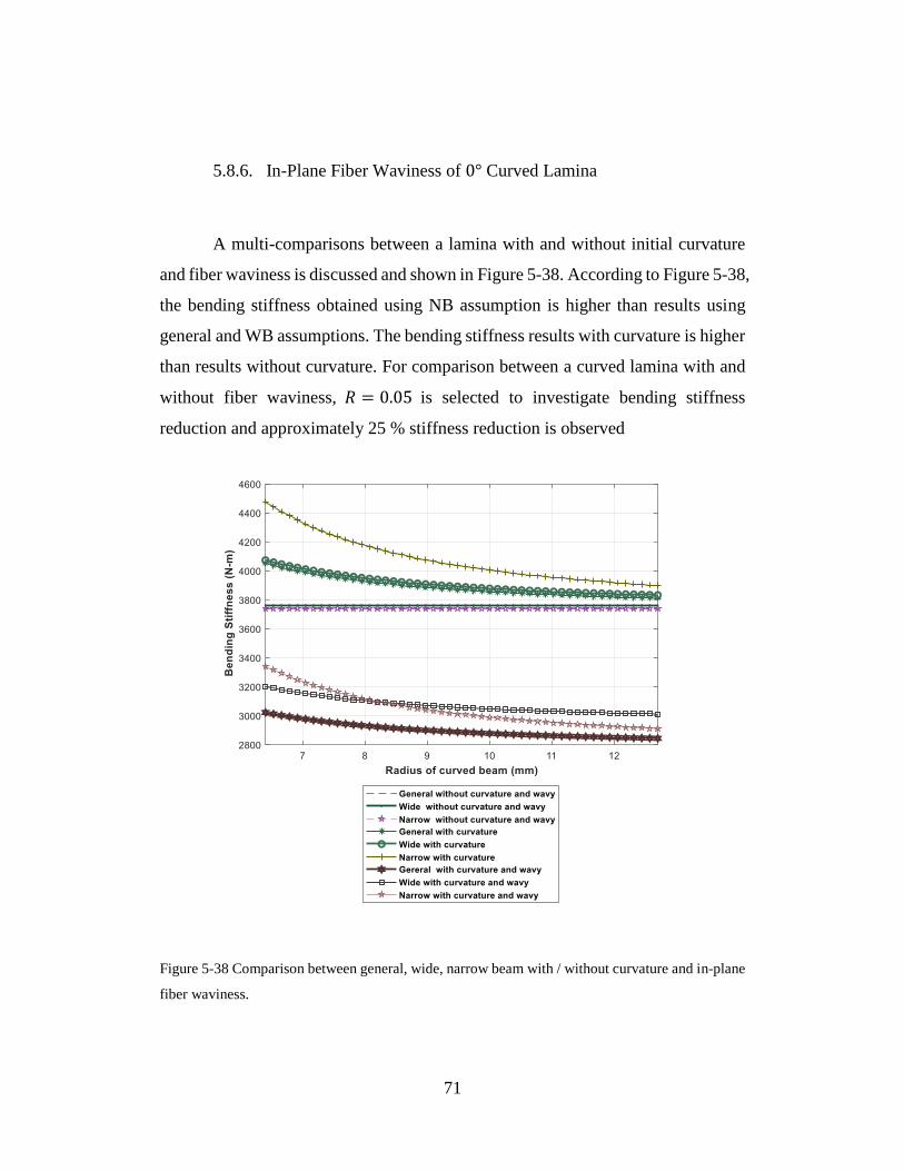
71

5.8.6. In-Plane Fiber Waviness of 0° Curved Lamina

A multi-comparisons between a lamina with and without initial curvature

and fiber waviness is discussed and shown in Figure 5-38. According to Figure 5-38,

the bending stiffness obtained using NB assumption is higher than results using

general and WB assumptions. The bending stiffness results with curvature is higher

than results without curvature. For comparison between a curved lamina with and

without fiber waviness, 𝑅 = 0.05 is selected to investigate bending stiffness

reduction and approximately 25 % stiffness reduction is observed

Figure 5-38 Comparison between general, wide, narrow beam with / without curvature and in-plane

fiber waviness.

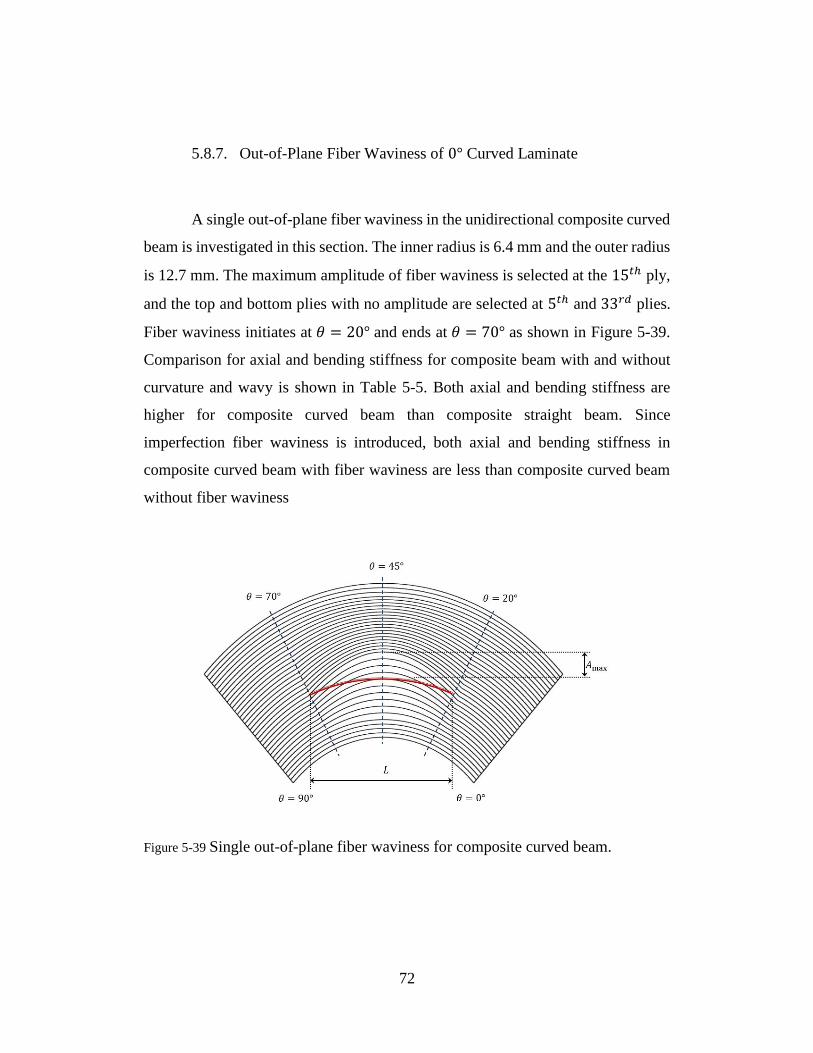
72

5.8.7. Out-of-Plane Fiber Waviness of 0° Curved Laminate

A single out-of-plane fiber waviness in the unidirectional composite curved

beam is investigated in this section. The inner radius is 6.4 mm and the outer radius

is 12.7 mm. The maximum amplitude of fiber waviness is selected at the 15𝑡ℎ ply,

and the top and bottom plies with no amplitude are selected at 5𝑡ℎ and 33𝑟𝑑 plies.

Fiber waviness initiates at 𝜃 = 20° and ends at 𝜃 = 70° as shown in Figure 5-39.

Comparison for axial and bending stiffness for composite beam with and without

curvature and wavy is shown in Table 5-5. Both axial and bending stiffness are

higher for composite curved beam than composite straight beam. Since

imperfection fiber waviness is introduced, both axial and bending stiffness in

composite curved beam with fiber waviness are less than composite curved beam

without fiber waviness

Figure 5-39 Single out-of-plane fiber waviness for composite curved beam.

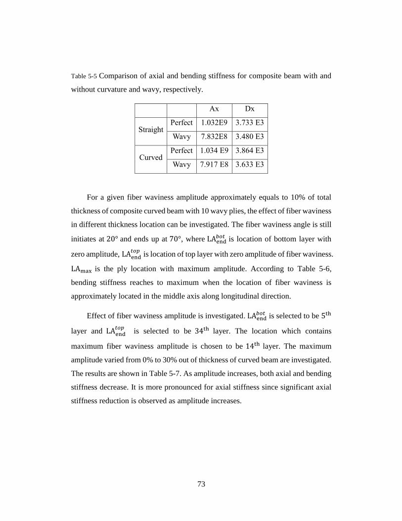
73

Table 5-5 Comparison of axial and bending stiffness for composite beam with and

without curvature and wavy, respectively.

Ax Dx

Straight Perfect 1.032E9 3.733 E3

Wavy 7.832E8 3.480 E3

Curved Perfect 1.034 E9 3.864 E3

Wavy 7.917 E8 3.633 E3

For a given fiber waviness amplitude approximately equals to 10% of total

thickness of composite curved beam with 10 wavy plies, the effect of fiber waviness

in different thickness location can be investigated. The fiber waviness angle is still

initiates at 20° and ends up at 70°, where LAend𝑏𝑜𝑡 is location of bottom layer with

zero amplitude, LAend𝑡𝑜𝑝

is location of top layer with zero amplitude of fiber waviness.

LAmax is the ply location with maximum amplitude. According to Table 5-6,

bending stiffness reaches to maximum when the location of fiber waviness is

approximately located in the middle axis along longitudinal direction.

Effect of fiber waviness amplitude is investigated. LAend𝑏𝑜𝑡 is selected to be 5th

layer and LAend𝑡𝑜𝑝

is selected to be 34th layer. The location which contains

maximum fiber waviness amplitude is chosen to be 14th layer. The maximum

amplitude varied from 0% to 30% out of thickness of curved beam are investigated.

The results are shown in Table 5-7. As amplitude increases, both axial and bending

stiffness decrease. It is more pronounced for axial stiffness since significant axial

stiffness reduction is observed as amplitude increases.

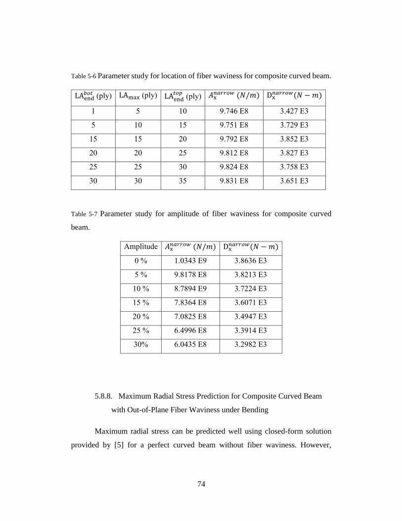
74

Table 5-6 Parameter study for location of fiber waviness for composite curved beam.

LAend𝑏𝑜𝑡 (ply) LAmax (ply) LAend

𝑡𝑜𝑝 (ply) 𝐴x

𝑛𝑎𝑟𝑟𝑜𝑤 (𝑁/𝑚) Dx𝑛𝑎𝑟𝑟𝑜𝑤(𝑁 −𝑚)

1 5 10 9.746 E8 3.427 E3

5 10 15 9.751 E8 3.729 E3

15 15 20 9.792 E8 3.852 E3

20 20 25 9.812 E8 3.827 E3

25 25 30 9.824 E8 3.758 E3

30 30 35 9.831 E8 3.651 E3

Table 5-7 Parameter study for amplitude of fiber waviness for composite curved

beam.

Amplitude 𝐴x𝑛𝑎𝑟𝑟𝑜𝑤 (𝑁/𝑚) Dx

𝑛𝑎𝑟𝑟𝑜𝑤(𝑁 − 𝑚)

0 % 1.0343 E9 3.8636 E3

5 % 9.8178 E8 3.8213 E3

10 % 8.7894 E9 3.7224 E3

15 % 7.8364 E8 3.6071 E3

20 % 7.0825 E8 3.4947 E3

25 % 6.4996 E8 3.3914 E3

30% 6.0435 E8 3.2982 E3

5.8.8. Maximum Radial Stress Prediction for Composite Curved Beam

with Out-of-Plane Fiber Waviness under Bending

Maximum radial stress can be predicted well using closed-form solution

provided by [5] for a perfect curved beam without fiber waviness. However,

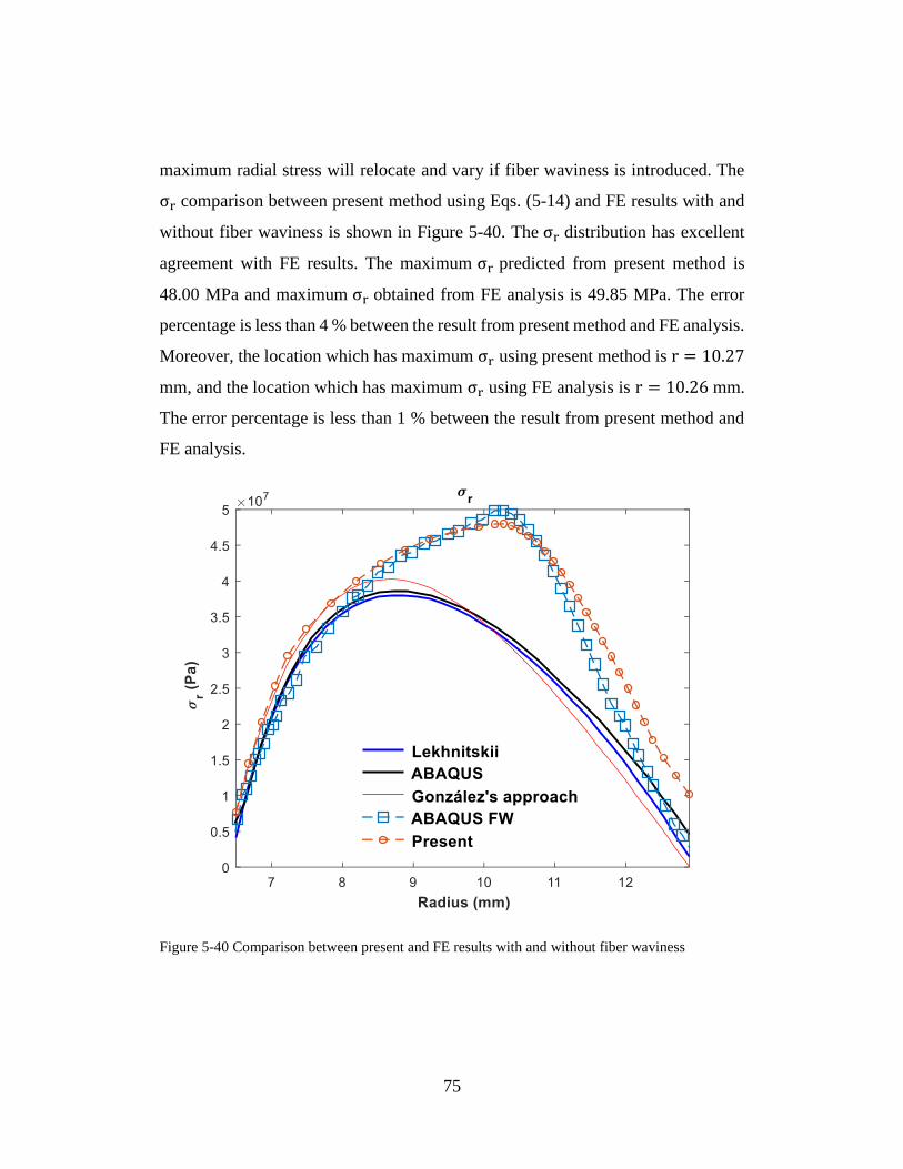
75

maximum radial stress will relocate and vary if fiber waviness is introduced. The

σr comparison between present method using Eqs. (5-14) and FE results with and

without fiber waviness is shown in Figure 5-40. The σr distribution has excellent

agreement with FE results. The maximum σr predicted from present method is

48.00 MPa and maximum σr obtained from FE analysis is 49.85 MPa. The error

percentage is less than 4 % between the result from present method and FE analysis.

Moreover, the location which has maximum σr using present method is r = 10.27

mm, and the location which has maximum σr using FE analysis is r = 10.26 mm.

The error percentage is less than 1 % between the result from present method and

FE analysis.

Figure 5-40 Comparison between present and FE results with and without fiber waviness

76

5-9 Conclusion

A closed-form analytical solution is developed for analyzing laminated

composite beam with and without initial curvature and fiber waviness, respectively.

The explicit expressions for evaluating axial and bending stiffness are formulated

based upon modified lamination theory and taking into consideration the structural

deformation characteristics of beam with narrow section. Closed-form solutions are

also provided to analyze composite beam with in-plane and out-of-plane fiber

waviness. Incremental loading schematic is introduced and a practical iteration

number is selected. FE analysis is conducted to verify results using present

approach. The maximum radial stress for a composite curved beam with out-of-

plane fiber waviness under bending is discussed. The present stiffness and stress

results are in good agreement with numerical results obtained from ANAQUS. It is

found that the geometry of fiber waviness such as location where has maximum

amplitude and the maximum amplitude of fiber waviness has a great impact on

equivalent axial and bending stiffness. However, fiber waviness has less impact on

the bending stiffness of plies affected by fiber waviness are near the middle axis of

the composite curved beam. It is concluded that the present approach can provide

an efficient method for analyzing laminated composite curved beam with in-plane

and out-of-plane fiber waviness.

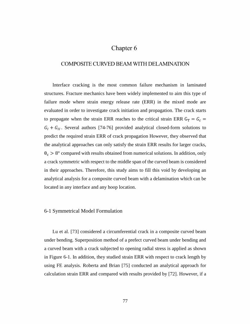
77

COMPOSITE CURVED BEAM WITH DELAMINATION

Interface cracking is the most common failure mechanism in laminated

structures. Fracture mechanics have been widely implemented to aim this type of

failure mode where strain energy release rate (ERR) in the mixed mode are

evaluated in order to investigate crack initiation and propagation. The crack starts

to propagate when the strain ERR reaches to the critical strain ERR GT = 𝐺𝑐 =

𝐺𝐼 + 𝐺𝐼𝐼 . Several authors [74-76] provided analytical closed-form solutions to

predict the required strain ERR of crack propagation However, they observed that

the analytical approaches can only satisfy the strain ERR results for larger cracks,

θc > 8° compared with results obtained from numerical solutions. In addition, only

a crack symmetric with respect to the middle span of the curved beam is considered

in their approaches. Therefore, this study aims to fill this void by developing an

analytical analysis for a composite curved beam with a delamination which can be

located in any interface and any hoop location.

6-1 Symmetrical Model Formulation

Lu et al. [73] considered a circumferential crack in a composite curved beam

under bending. Superposition method of a prefect curved beam under bending and

a curved beam with a crack subjected to opening radial stress is applied as shown

in Figure 6-1. In addition, they studied strain ERR with respect to crack length by

using FE analysis. Roberta and Brian [75] conducted an analytical approach for

calculation strain ERR and compared with results provided by [72]. However, if a

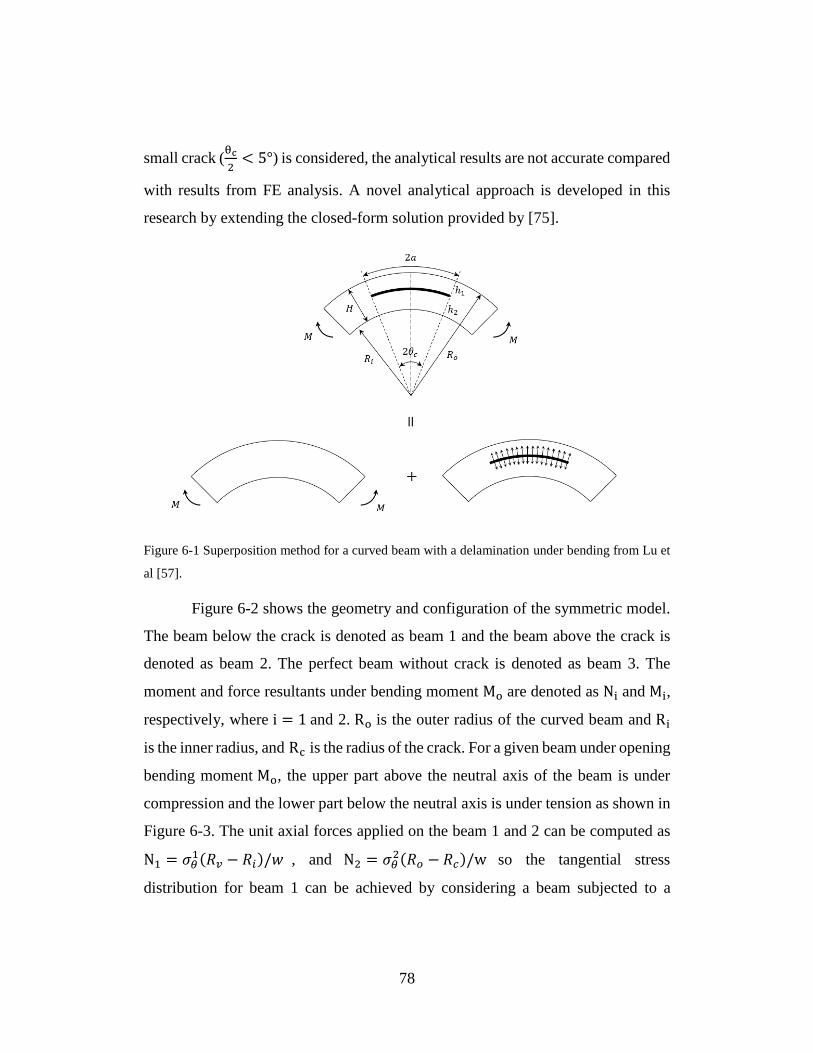
78

small crack (θc

2< 5°) is considered, the analytical results are not accurate compared

with results from FE analysis. A novel analytical approach is developed in this

research by extending the closed-form solution provided by [75].

Figure 6-1 Superposition method for a curved beam with a delamination under bending from Lu et

al [57].

Figure 6-2 shows the geometry and configuration of the symmetric model.

The beam below the crack is denoted as beam 1 and the beam above the crack is

denoted as beam 2. The perfect beam without crack is denoted as beam 3. The

moment and force resultants under bending moment Mo are denoted as Ni and Mi,

respectively, where i = 1 and 2. Ro is the outer radius of the curved beam and Ri

is the inner radius, and Rc is the radius of the crack. For a given beam under opening

bending moment Mo, the upper part above the neutral axis of the beam is under

compression and the lower part below the neutral axis is under tension as shown in

Figure 6-3. The unit axial forces applied on the beam 1 and 2 can be computed as

N1 = 𝜎𝜃1(𝑅𝑣 − 𝑅𝑖)/𝑤 , and N2 = 𝜎𝜃

2(𝑅𝑜 − 𝑅𝑐)/w so the tangential stress

distribution for beam 1 can be achieved by considering a beam subjected to a

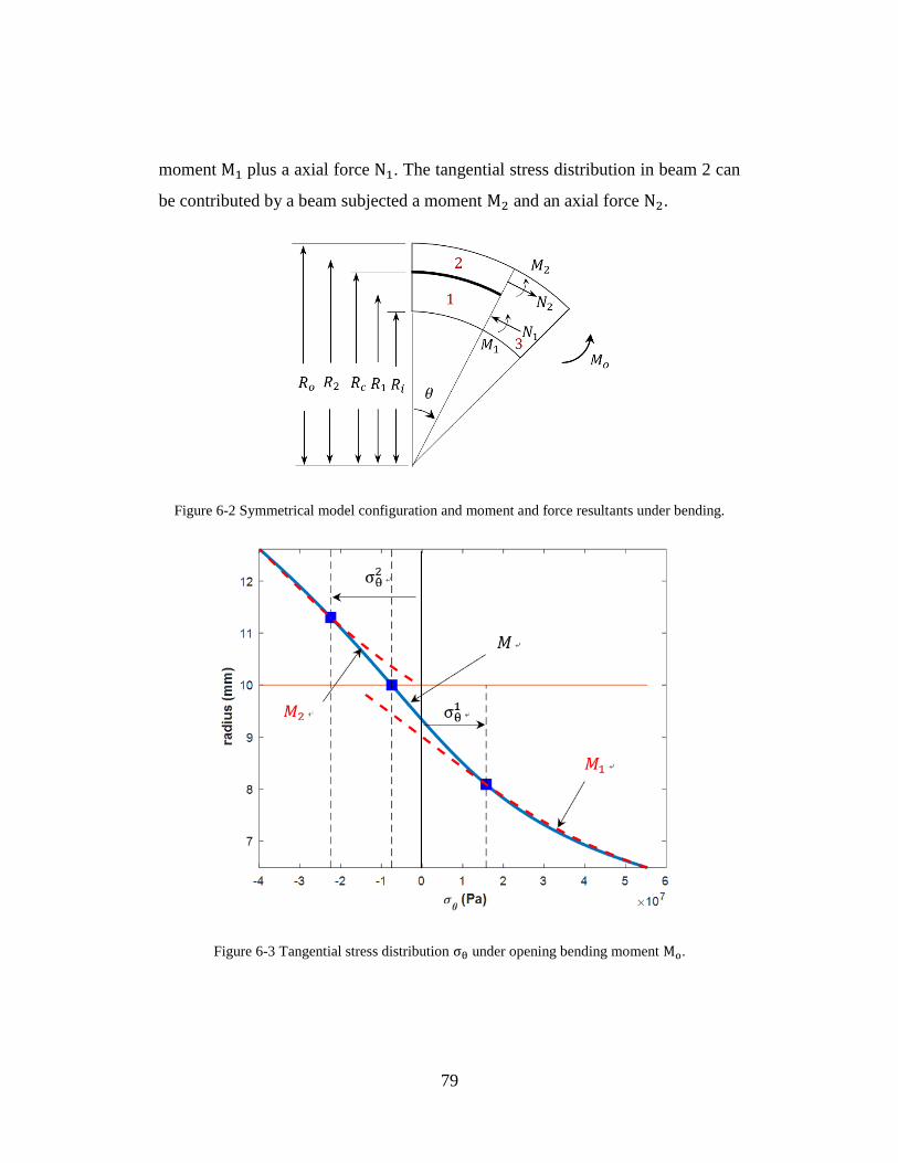
79

moment M1 plus a axial force N1. The tangential stress distribution in beam 2 can

be contributed by a beam subjected a moment M2 and an axial force N2.

Figure 6-2 Symmetrical model configuration and moment and force resultants under bending.

Figure 6-3 Tangential stress distribution σθ under opening bending moment Mo.

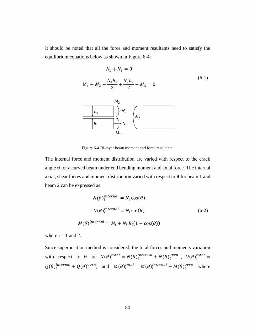
80

It should be noted that all the force and moment resultants need to satisfy the

equilibrium equations below as shown in Figure 6-4:

𝑁1 + 𝑁2 = 0

M1 +𝑀2 −𝑁1ℎ12

+𝑁2ℎ22

−𝑀3 = 0

(6-1)

Figure 6-4 Bi-layer beam moment and force resultants.

The internal force and moment distribution are varied with respect to the crack

angle θ for a curved beam under end bending moment and axial force. The internal

axial, shear forces and moment distribution varied with respect to θ for beam 1 and

beam 2 can be expressed as

𝑁(𝜃)𝑖𝑖𝑛𝑡𝑒𝑟𝑛𝑎𝑙 = 𝑁𝑖 cos(𝜃)

𝑄(𝜃)𝑖𝑖𝑛𝑡𝑒𝑟𝑛𝑎𝑙 = 𝑁𝑖 sin(𝜃)

𝑀(𝜃)𝑖𝑖𝑛𝑡𝑒𝑟𝑛𝑎𝑙 = 𝑀𝑖 + 𝑁𝑖 𝑅𝑖(1 − cos(𝜃))

(6-2)

where i = 1 and 2.

Since superposition method is considered, the total forces and moments variation

with respect to θ are 𝑁(𝜃)𝑖𝑡𝑜𝑡𝑎𝑙 = 𝑁(𝜃)𝑖

𝑖𝑛𝑡𝑒𝑟𝑛𝑎𝑙 + 𝑁(𝜃)𝑖𝑜𝑝𝑒𝑛

, 𝑄(𝜃)𝑖𝑡𝑜𝑡𝑎𝑙 =

𝑄(𝜃)𝑖𝑖𝑛𝑡𝑒𝑟𝑛𝑎𝑙 + 𝑄(𝜃)𝑖

𝑜𝑝𝑒𝑛, and 𝑀(𝜃)𝑖𝑡𝑜𝑡𝑎𝑙 = 𝑀(𝜃)𝑖

𝑖𝑛𝑡𝑒𝑟𝑛𝑎𝑙 +𝑀(𝜃)𝑖𝑜𝑝𝑒𝑛

where

81

𝑁(𝜃)𝑖𝑜𝑝𝑒𝑛, 𝑄(𝜃)𝑖

𝑜𝑝𝑒𝑛,𝑀(𝜃)𝑖𝑜𝑝𝑒𝑛

are axial force, shear force and moment due to

opening stress mentioned in Figure 6-1.

𝑁(𝜃)𝑖𝑜𝑝𝑒𝑛 = −𝑞𝑖 sin(𝜃/2)

𝑄(𝜃)𝑖𝑜𝑝𝑒𝑛 = 𝑞𝑖 cos(𝜃/2)

𝑀(𝜃)𝑖𝑜𝑝𝑒𝑛 = −𝑞𝑖𝑅𝑖 sin(𝜃/2 )

(6-2)

where 𝑞𝑖 = σr(𝑟) 𝑅𝑖𝜃, i = 1 and 2. σr(𝑟) can be found in Eqs. (4-16).

Thus, the total strain energy release rate can be obtained by following equation:

𝐺𝑇(𝜃) =1

2𝑅𝑐{𝑅1 (

𝑁(𝜃)1𝑡𝑜𝑡𝑎𝑙2

𝐸𝐴1+𝑀(𝜃)1

𝑡𝑜𝑡𝑎𝑙2

𝐸𝐼1+𝑄(𝜃)1


𝐺𝐴1)

+ 𝑅2 (𝑁(𝜃)2






𝐺𝐴2)

− 𝑅3 (𝑀𝑜2

𝐸𝐼3)}

(6-3)

where EA, EI, and GA are effective axial stiffness, bending stiffness, and shear

stiffness in Eqs. (4-5) and (4-6). It should be noticed unit forces and unit moment

are assumed in Eqs. (6-3). However, Eqs. (6-3) cannot accurately predict total strain

ERR. Therefore, a modified equation 𝐺𝑇𝑚(𝜃) based on non-dimensional

coefficients is proposed by comparing results obtained from Eqs. (6-3) and results

obtained from FE analysis.

82

𝐺𝑇𝑚(𝜃) = 𝛼 𝛽 𝐺𝑇(𝜃) (6-4)

The coefficient α is a parameter related to radial effect of crack location and the

coefficient β is a parameter related to crack length effect.

𝛼 = −25.254𝑅𝑝5 + 90.6𝑅𝑝4 − 101.29𝑅𝑝

3 + 36.879𝑅𝑝2 − 1.5689𝑅𝑝 + 3.5294

β =−(𝑦1) log(𝜃) + (𝑦2)

𝑦3

(6-5)

where

y1 = (0.007006𝑡2 + 0.6156356𝑡 − 0.2455147) (6-6)

y2 = 0.26848𝑡2 + 1.102285𝑡 + 4.3770866

y3 = −(𝑦1) log(16.6) + (𝑦2)

and t is the total thickness of composite curved beam in the unit of (mm). θ is the

crack angle in the unit of (degree), and Rp is the crack location ratio where Rp =

(𝑅𝑐 − 𝑅𝑖)/(𝑅𝑜 − 𝑅𝑖)

6-2 Unsymmetrical Model Formulation

The configuration of unsymmetrical model is shown in Figure 6-5. θh is the

hoop angle locating with respect to the middle length of the crack. The angle of left

crack tip is denoted as θs. The angle of right crack tip is denoted as θe, where s is

start angle, and e is end angle of the crack where θh = (𝜃𝑠 + 𝜃𝑒)/2. The lower part

of the beam is denoted as beam 1, and the upper part of the beam is denoted as

beam 2. Beam 3 and 4 are beams without crack as shown in Figure 6-5. Considering

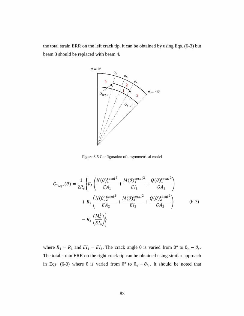
83

the total strain ERR on the left crack tip, it can be obtained by using Eqs. (6-3) but

beam 3 should be replaced with beam 4.

Figure 6-5 Configuration of unsymmetrical model

𝐺𝑇𝑙𝑒𝑓𝑡(𝜃) =1

2𝑅𝑐{𝑅1 (

𝑁(𝜃)1𝑡𝑜𝑡𝑎𝑙2





𝐺𝐴1)

+ 𝑅2 (𝑁(𝜃)2






𝐺𝐴2)

− 𝑅4 (𝑀𝑜2

𝐸𝐼4)}

(6-7)

where 𝑅4 = 𝑅3 and 𝐸𝐼4 = 𝐸𝐼3. The crack angle θ is varied from 0° to θh − 𝜃𝑠 .

The total strain ERR on the right crack tip can be obtained using similar approach

in Eqs. (6-3) where θ is varied from 0° to θe − 𝜃ℎ . It should be noted that

84

regularized model is applied for a curved beam with a small initial curvature only.

The stress distribution for a curved composite beam under bending is assumed to

be independent of θ if regularized model is considered. However, if moderate and

large initial curvatures are considered for a curved beam under bending, non-

regularized model has to be applied. The stress distribution of non-regularized

model is assumed to be independent of θ within a certain range. According to

González [82], the non-regularized angle θnr = 23.32° is introduced for a

composite curved beam where the radius to thickness ratio is 1.5. This ratio is

similar to the ratio applied in the present approach, which is 1.51. Based on their

model, a linear equation to describe reduced σr which is a function of crack angle

θck is introduced as

σr𝑛𝑒𝑤 = 𝜎𝑟 P

P = (−2.29277 θ𝑐𝑘 + 148.174)/100

(6-8)

where P is the percentage, θck is the crack angle in the unit of degree. According to

their σr results, for a given interface but varied with hoop angle, σr remains

constant until θ = θnr, and starts to decrease 52 % when θ = 45°. Linear variation

of P is assumed as shown in Eqs. (6-8).

The strain ERR based on beam 1, 2, and 4 has higher value compared to the

one in the right composed by beam 1, 2, and 3 under end bending moment. The

equivalent force per unit width due to opening stress σr within the region where

θs < 𝜃 < 𝜃ℎ and θs > 𝜃𝑛𝑟 can be written as

𝑞𝑖𝑙𝑒𝑓𝑡 = σrleft𝑛𝑒𝑤 𝑅𝑖𝜃 (6-9)

where θ is varied from 0° to θh − 𝜃𝑠 , i = 1 and 2. σrleft𝑛𝑒𝑤 = 𝜎𝑟 𝑃 , where

θck is (θs+θh)/2. The equivalent force per unit width due to opening stress σr

within the region where θh < 𝜃 < 𝜃𝑒 and θs > 𝜃𝑛𝑟 can be written as

85

𝑞𝑖𝑟𝑖𝑔ℎ𝑡 = σr𝑟𝑖𝑔ℎ𝑡𝑛𝑒𝑤 𝑅𝑖𝜃 (6-10)

where θ is varied from 0° to θe − 𝜃ℎ , i = 1 and 2. σr𝑟𝑖𝑔ℎ𝑡𝑛𝑒𝑤 = 𝜎𝑟 𝑃 , where

θck is (θh + θe)/2. Once reduced 𝑞𝑖 is obtained, the total strain ERR for a crack

locates in any hoop location is obtained using Eqs. (6-2) to (6-4).

6-3 Finite Element Analysis

An ABAQUS based non-linear FE analysis is developed to simulate structural

response of a composite curved beam with a crack. The failure load under bending,

and the strain ERR in Mode I and II are investigated. A unidirectional laminated

curved beam is considered. The inner radius of the curved beam is 6.4 mm and the

outer radius 12.7 mm. The width of the beam is 12.7 mm. IM7/8552 carbon-epoxy

composite material properties are implemented.

6.3.1. Model Formulation

Delamination is located at the interface between upper and lower laminates.

Thus, two sub-laminate system is implemented in order to simulate delamination

using Virtual Crack Closure Technique (VCCT) [85]. The upper surface of the

lower beam is chosen as the master surface and the lower surface of the upper beam

is chosen as the slave surface as shown in Figure 6-6. Discrete material orientation

is considered since unidirectional laminated beam is implemented as shown in

Figure 6-6, where 1 is the fiber direction. During mesh process, it should be noticed

that element numbers between slave surface and master surface has to be identical

because nodes on the master and slave surfaces will be bonded. The bonded node

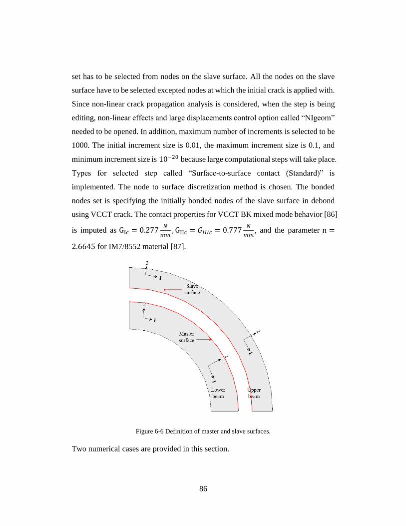
86

set has to be selected from nodes on the slave surface. All the nodes on the slave

surface have to be selected excepted nodes at which the initial crack is applied with.

Since non-linear crack propagation analysis is considered, when the step is being

editing, non-linear effects and large displacements control option called “NIgeom”

needed to be opened. In addition, maximum number of increments is selected to be

1000. The initial increment size is 0.01, the maximum increment size is 0.1, and

minimum increment size is 10−20 because large computational steps will take place.

Types for selected step called “Surface-to-surface contact (Standard)” is

implemented. The node to surface discretization method is chosen. The bonded

nodes set is specifying the initially bonded nodes of the slave surface in debond

using VCCT crack. The contact properties for VCCT BK mixed mode behavior [86]

is imputed as GIc = 0.277𝑁

𝑚𝑚, GIIc = 𝐺𝐼𝐼𝐼𝑐 = 0.777

𝑁

𝑚𝑚, and the parameter n =

2.6645 for IM7/8552 material [87].

Figure 6-6 Definition of master and slave surfaces.

Two numerical cases are provided in this section.

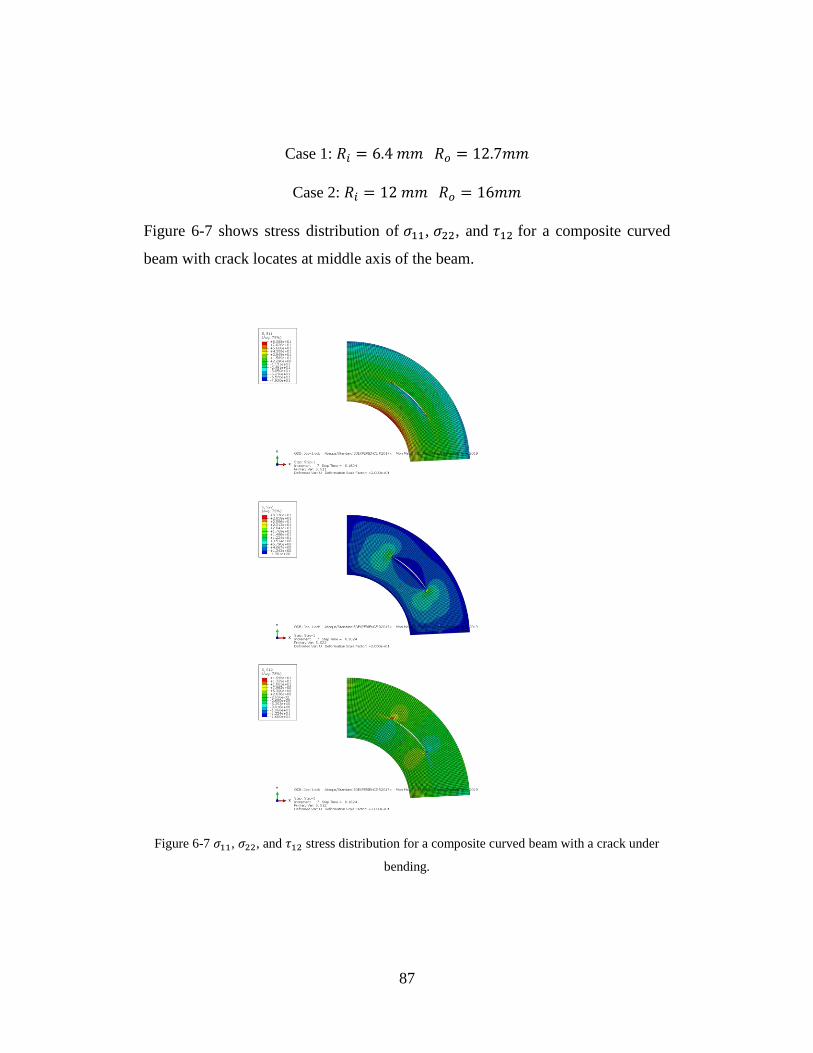
87

Case 1: 𝑅𝑖 = 6.4 𝑚𝑚 𝑅𝑜 = 12.7𝑚𝑚

Case 2: 𝑅𝑖 = 12 𝑚𝑚 𝑅𝑜 = 16𝑚𝑚

Figure 6-7 shows stress distribution of 𝜎11, 𝜎22, and 𝜏12 for a composite curved

beam with crack locates at middle axis of the beam.

Figure 6-7 𝜎11, 𝜎22, and 𝜏12 stress distribution for a composite curved beam with a crack under

bending.

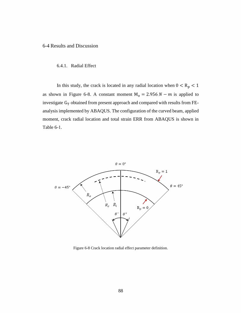
88


6.4.1. Radial Effect

In this study, the crack is located in any radial location when 0 < Rp < 1

as shown in Figure 6-8. A constant moment Mo = 2.956 𝑁 −𝑚 is applied to

investigate GT obtained from present approach and compared with results from FE-

analysis implemented by ABAQUS. The configuration of the curved beam, applied

moment, crack radial location and total strain ERR from ABAQUS is shown in

Table 6-1.

Figure 6-8 Crack location radial effect parameter definition.

89

Table 6-1 Crack location radial effect parameters and strain ERR results obtained from FE analysis

(case 1).

𝜃+ 𝜃− 𝑅𝑖 𝑅𝑜 𝑅𝑐 𝑅𝑝 𝑀𝑜 𝐺𝐼𝐹𝐸 𝐺𝐼𝐼

𝐹𝐸 𝐺𝐼𝐹𝐸

𝐺𝐼𝐼𝐹𝐸 𝐺𝑇

𝐹𝐸

16.2 -16.2 6.4 12.7 7.03 10% 2956 134.167 3.68 2.74% 137.85

16.2 -16.2 6.4 12.7 7.66 20% 2956 201.85 8.8 4.36% 210.65

16.2 -16.2 6.4 12.7 8.29 30% 2956 244.512 14.04 5.74% 258.55

16.2 -16.2 6.4 12.7 8.92 40% 2956 260.695 18.15 6.96% 278.85

16.2 -16.2 6.4 12.7 9.55 50% 2956 245.735 20.36 8.29% 266.10

16.2 -16.2 6.4 12.7 10.18 60% 2956 204.205 20.78 10.18% 224.99

16.2 -16.2 6.4 12.7 10.81 70% 2956 148.029 20.28 13.70% 168.31

16.2 -16.2 6.4 12.7 11.44 80% 2956 89.06 19.96 22.41% 109.02

16.2 -16.2 6.4 12.7 12.07 90% 2956 33.65 20.52 60.98% 54.17

where the unit of radius is mm, the unit of moment is N-mm, the unit of θ is in

degree, and the unit of strain ERR is 𝑁/𝑚.

The total strain ERR comparison between present method and results

obtained from ABAQUS is tabulated in Table 6-2. 𝐺𝑇𝑝

is the total strain ERR

obtained from present method, and 𝐺𝑇𝐹𝐸 is the total strain ERR using FE analysis

implemented by ABAQUS. The comparison is also shown in Figure 6-9. All the

results obtained from present method have excellent agreement with ABAQUS’s

results except when Rp = 0.1.

The geometry and applied moment in second case are tabulated in Table

6-3. The comparison between the total strain ERR results obtained from the present

method and ABAQUS are tabulated in Table 6-4 and is shown in Figure 6-10. The

total strain energy increase as Rp increases. It reaches to maximum when Rp ≅

0.33. It should be more pronounced that the crack is located near the neutral axis

of the curved beam. In conclusion, the present method has excellent accuracy at

90

predicting the total strain ERR results where the crack can be located in any radial

interface.

Table 6-2 Total strain ERR comparison between present method and ABAQUS (case 1).

𝜃+ 𝜃− 𝑅𝑖 𝑅𝑜 𝑅𝑐 𝑅𝑝 𝑀𝑜 𝐺𝑇𝑝

𝐺𝑇𝐹𝐸 % Diff.

16.2 -16.2 6.4 12.7 7.03 10% 2956 137.85 125 9.32%

16.2 -16.2 6.4 12.7 7.66 20% 2956 210.65 213 -1.12%

16.2 -16.2 6.4 12.7 8.29 30% 2956 258.55 252 2.53%

16.2 -16.2 6.4 12.7 8.92 40% 2956 278.85 269 3.53%

16.2 -16.2 6.4 12.7 9.55 50% 2956 266.10 253 4.92%

16.2 -16.2 6.4 12.7 10.18 60% 2956 224.99 219 2.66%

16.2 -16.2 6.4 12.7 10.81 70% 2956 168.31 164 2.56%

16.2 -16.2 6.4 12.7 11.44 80% 2956 109.02 116 -6.40%

16.2 -16.2 6.4 12.7 12.07 90% 2956 54.17 56.3 -3.93%

Figure 6-9 GT comparison between present method and ABAQUS (case 1).

91

Table 6-3 Crack location radial effect parameters and strain ERR results obtained from FE analysis

(case 2).

𝜃+ 𝜃− 𝑅𝑖 𝑅𝑜 𝑅𝑐 𝑅𝑝 𝑀𝑜 𝐺𝐼𝐹𝐸 𝐺𝐼𝐼



𝐹𝐸

16.2 -16.2 12 16 12.4 10% 1497 89.764 3.51 3.91% 93.27

16.2 -16.2 12 16 12.8 20% 1497 199.933 4.52 2.26% 204.45

16.2 -16.2 12 16 13.2 30% 1497 255.985 9.24 3.61% 265.23

16.2 -16.2 12 16 13.6 40% 1497 268.702 16.15 6.01% 290.24

16.2 -16.2 12 16 14 50% 1497 246.51 23.63 9.59% 277.14

16.2 -16.2 12 16 14.4 60% 1497 200.662 30.82 15.36% 231.48

16.2 -16.2 12 16 14.8 70% 1497 142.296 37.56 26.40% 179.86

16.2 -16.2 12 16 15.2 80% 1497 79.48 43.35 54.54% 122.83

16.2 -16.2 12 16 15.6 90% 1497 18.77 39.23 209.00% 58.00


𝜃+ 𝜃− 𝑅𝑖 𝑅𝑜 𝑅𝑐 𝑅𝑝 𝑀𝑜 𝐺𝑇𝑝

𝐺𝑇𝐹𝐸 % Diff.

16.2 -16.2 12 16 12.4 10% 1497 103 93.27 -10.43%

16.2 -16.2 12 16 12.8 20% 1497 206 204.45 -0.76%

16.2 -16.2 12 16 13.2 30% 1497 265 265.23 0.08%

16.2 -16.2 12 16 13.6 40% 1497 299 290.24 -3.02%

16.2 -16.2 12 16 14 50% 1497 285 277.14 -2.84%

16.2 -16.2 12 16 14.4 60% 1497 243 231.48 -4.98%

16.2 -16.2 12 16 14.8 70% 1497 177 179.86 1.59%

16.2 -16.2 12 16 15.2 80% 1497 120 122.83 2.30%

16.2 -16.2 12 16 15.6 90% 1497 55.5 58.00 4.31%

92

Figure 6-10 GT comparison between present method and ABAQUS (case 2).

6.4.2. Length Effect

For case 1, the crack radius is 10 mm. A constant moment Mo = 2 𝑁 −𝑚

is applied to investigate GT obtained from present approach and compared with

results from FE-analysis implemented by ABAQUS. The configuration of the

curved beam, applied moment, crack radial location and total strain ERR from

ABAQUS is shown in Table 6-5. The total strain ERR comparison between present

method and results obtained from ABAQUS is tabulated in Table 6-6. 𝐺𝑇𝑝 is the total

strain ERR obtained from present method, and 𝐺𝑇𝐹𝐸 is the total strain ERR using FE

analysis implemented by ABAQUS. The comparison is also shown in Figure 6-11Figure

93

6-9. All the results obtained from present method have excellent agreement with

ABAQUS’s results especially for small crack.

Table 6-5 Crack length effect parameters and strain ERR results obtained from FE analysis (case 1).

𝜃+ 𝜃− 𝑅𝑖 𝑅𝑜 𝑅𝑐 𝑀𝑜 𝐺𝐼𝐹𝐸 𝐺𝐼𝐼



𝐹𝐸

2.70 -2.70 6.4 12.7 10 2000 17.61 0 0.00% 17.61

5.40 -5.40 6.4 12.7 10 2000 37.6 0.46 1.22% 38.06

8.10 -8.10 6.4 12.7 10 2000 56.86 1.51 2.66% 58.37

10.80 -10.80 6.4 12.7 10 2000 74.74 3.55 4.75% 78.29

13.50 -13.50 6.4 12.7 10 2000 89.87 6.8 7.57% 96.67

16.20 -16.20 6.4 12.7 10 2000 101 11.3 11.19% 112.3


𝜃+ 𝜃− 𝑅𝑖 𝑅𝑜 𝑅𝑐 𝑀𝑜 𝐺𝑇𝑝 𝐺𝑇

𝐹𝐸 % Diff.

2.70 -2.70 6.4 12.7 10 2000 17.2 17.61 2.33%

5.40 -5.40 6.4 12.7 10 2000 37.4 38.06 1.73%

8.10 -8.10 6.4 12.7 10 2000 60.7 58.37 -3.99%

10.80 -10.80 6.4 12.7 10 2000 82.4 78.29 -5.25%

13.50 -13.50 6.4 12.7 10 2000 99.7 96.67 -3.13%

16.20 -16.20 6.4 12.7 10 2000 110 112.3 2.05%

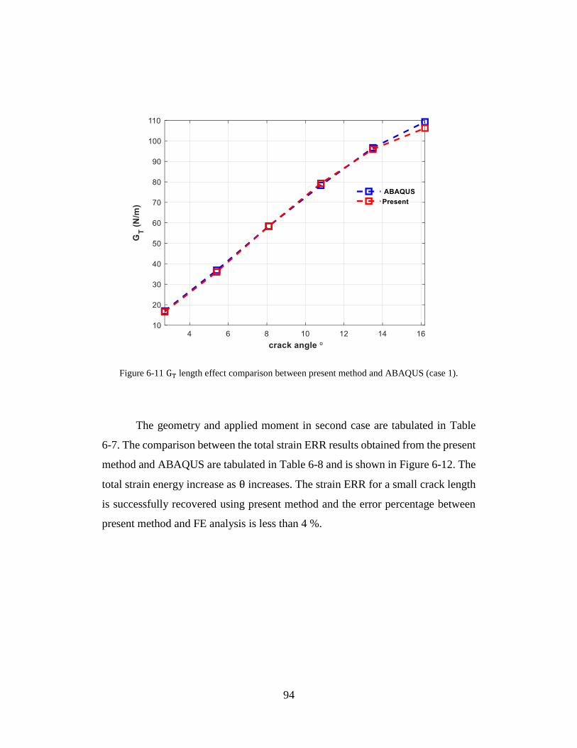
94

Figure 6-11 GT length effect comparison between present method and ABAQUS (case 1).

The geometry and applied moment in second case are tabulated in Table

6-7. The comparison between the total strain ERR results obtained from the present

method and ABAQUS are tabulated in Table 6-8 and is shown in Figure 6-12. The

total strain energy increase as θ increases. The strain ERR for a small crack length

is successfully recovered using present method and the error percentage between

present method and FE analysis is less than 4 %.

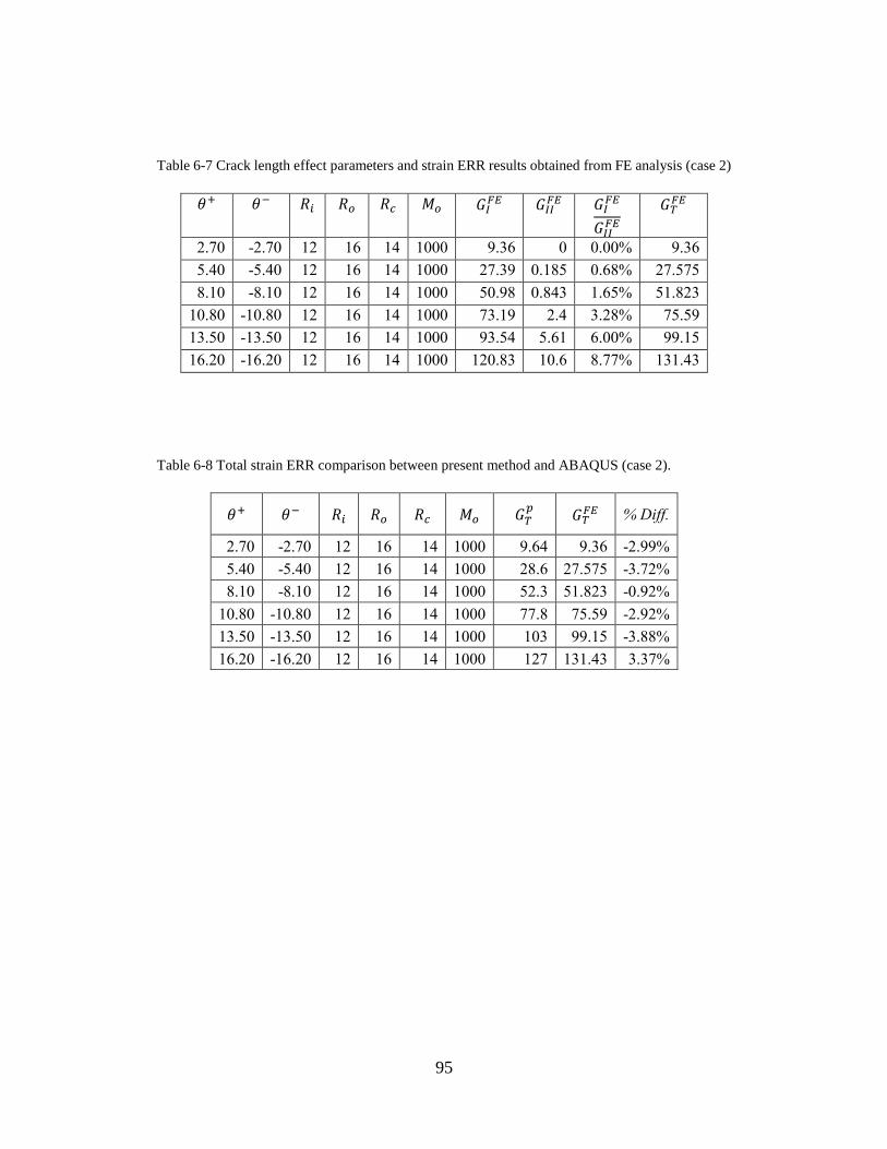
95

Table 6-7 Crack length effect parameters and strain ERR results obtained from FE analysis (case 2)

𝜃+ 𝜃− 𝑅𝑖 𝑅𝑜 𝑅𝑐 𝑀𝑜 𝐺𝐼𝐹𝐸 𝐺𝐼𝐼


𝐺𝐼𝐼𝐹𝐸

𝐺𝑇𝐹𝐸

2.70 -2.70 12 16 14 1000 9.36 0 0.00% 9.36

5.40 -5.40 12 16 14 1000 27.39 0.185 0.68% 27.575

8.10 -8.10 12 16 14 1000 50.98 0.843 1.65% 51.823

10.80 -10.80 12 16 14 1000 73.19 2.4 3.28% 75.59

13.50 -13.50 12 16 14 1000 93.54 5.61 6.00% 99.15

16.20 -16.20 12 16 14 1000 120.83 10.6 8.77% 131.43


𝜃+ 𝜃− 𝑅𝑖 𝑅𝑜 𝑅𝑐 𝑀𝑜 𝐺𝑇𝑝 𝐺𝑇

𝐹𝐸 % Diff.

2.70 -2.70 12 16 14 1000 9.64 9.36 -2.99%

5.40 -5.40 12 16 14 1000 28.6 27.575 -3.72%

8.10 -8.10 12 16 14 1000 52.3 51.823 -0.92%

10.80 -10.80 12 16 14 1000 77.8 75.59 -2.92%

13.50 -13.50 12 16 14 1000 103 99.15 -3.88%

16.20 -16.20 12 16 14 1000 127 131.43 3.37%

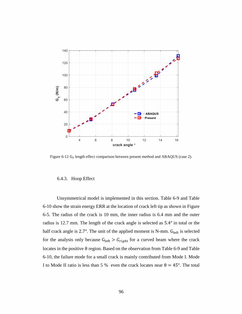
96

Figure 6-12 GT length effect comparison between present method and ABAQUS (case 2).

6.4.3. Hoop Effect

Unsymmetrical model is implemented in this section. Table 6-9 and Table

6-10 show the strain energy ERR at the location of crack left tip as shown in Figure

6-5. The radius of the crack is 10 mm, the inner radius is 6.4 mm and the outer

radius is 12.7 mm. The length of the crack angle is selected as 5.4° in total or the

half crack angle is 2.7°. The unit of the applied moment is N-mm. Gleft is selected

for the analysis only because Gleft > 𝐺𝑟𝑖𝑔ℎ𝑡 for a curved beam where the crack

locates in the positive θ region. Based on the observation from Table 6-9 and Table

6-10, the failure mode for a small crack is mainly contributed from Mode I. Mode

I to Mode II ratio is less than 5 % even the crack locates near θ = 45°. The total

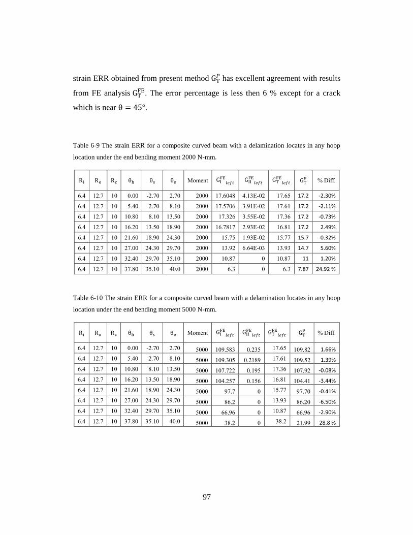
97

strain ERR obtained from present method GT𝑃 has excellent agreement with results

from FE analysis GTFE. The error percentage is less then 6 % except for a crack

which is near θ = 45°.

Table 6-9 The strain ERR for a composite curved beam with a delamination locates in any hoop

location under the end bending moment 2000 N-mm.

Ri Ro Rc θh θs θe Moment GIFE𝑙𝑒𝑓𝑡

GIIFE𝑙𝑒𝑓𝑡

GTFE𝑙𝑒𝑓𝑡

GT𝑝

% Diff.

6.4 12.7 10 0.00 -2.70 2.70 2000 17.6048 4.13E-02 17.65 17.2 -2.30%

6.4 12.7 10 5.40 2.70 8.10 2000 17.5706 3.91E-02 17.61 17.2 -2.11%

6.4 12.7 10 10.80 8.10 13.50 2000 17.326 3.55E-02 17.36 17.2 -0.73%

6.4 12.7 10 16.20 13.50 18.90 2000 16.7817 2.93E-02 16.81 17.2 2.49%

6.4 12.7 10 21.60 18.90 24.30 2000 15.75 1.93E-02 15.77 15.7 -0.32%

6.4 12.7 10 27.00 24.30 29.70 2000 13.92 6.64E-03 13.93 14.7 5.60%

6.4 12.7 10 32.40 29.70 35.10 2000 10.87 0 10.87 11 1.20%

6.4 12.7 10 37.80 35.10 40.0 2000 6.3 0 6.3 7.87 24.92 %

Table 6-10 The strain ERR for a composite curved beam with a delamination locates in any hoop

location under the end bending moment 5000 N-mm.

Ri Ro Rc θh θs θe Moment GIFE𝑙𝑒𝑓𝑡

GIIFE𝑙𝑒𝑓𝑡

GTFE𝑙𝑒𝑓𝑡

GT𝑝

% Diff.

6.4 12.7 10 0.00 -2.70 2.70 5000 109.583 0.235 17.65 109.82 1.66%

6.4 12.7 10 5.40 2.70 8.10 5000 109.305 0.2189 17.61 109.52 1.39%

6.4 12.7 10 10.80 8.10 13.50 5000 107.722 0.195 17.36 107.92 -0.08%

6.4 12.7 10 16.20 13.50 18.90 5000 104.257 0.156 16.81 104.41 -3.44%

6.4 12.7 10 21.60 18.90 24.30 5000 97.7 0 15.77 97.70 -0.41%

6.4 12.7 10 27.00 24.30 29.70 5000 86.2 0 13.93 86.20 -6.50%

6.4 12.7 10 32.40 29.70 35.10 5000 66.96 0 10.87 66.96 -2.90%

6.4 12.7 10 37.80 35.10 40.0 5000 38.2 0 38.2 21.99 28.8 %

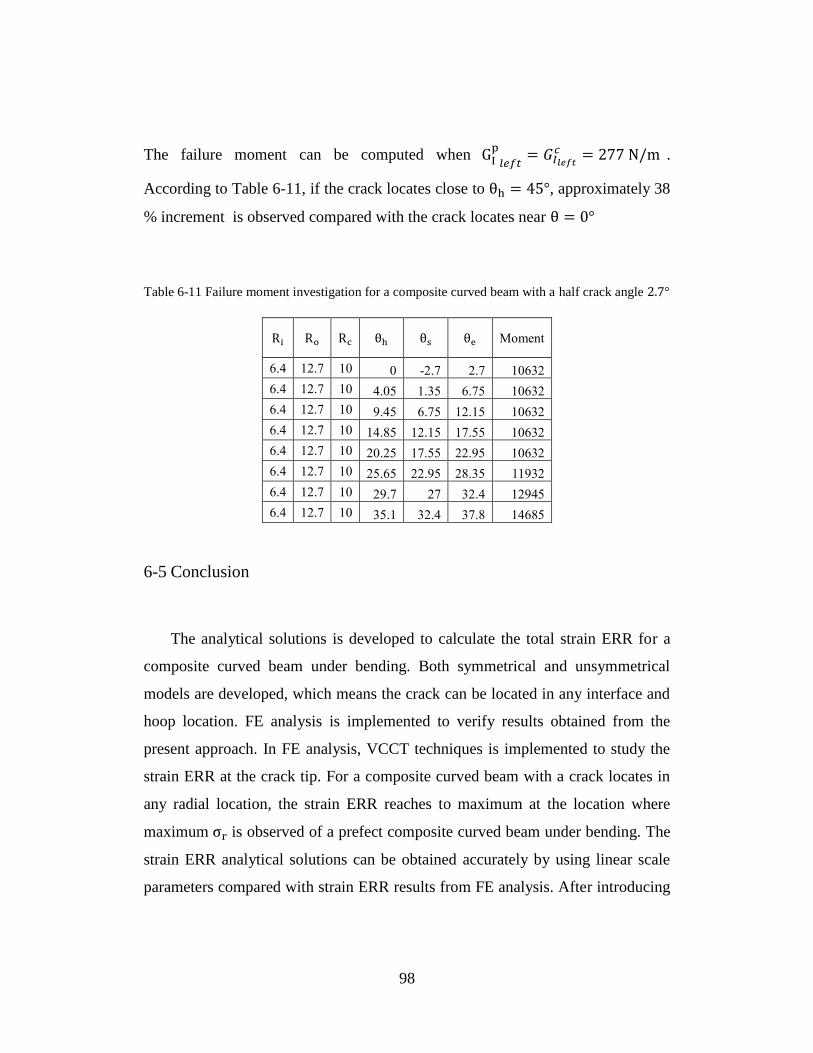
98

The failure moment can be computed when GIp

𝑙𝑒𝑓𝑡= 𝐺𝐼𝑙𝑒𝑓𝑡

𝑐 = 277 N/m .

According to Table 6-11, if the crack locates close to θh = 45°, approximately 38

% increment is observed compared with the crack locates near θ = 0°

Table 6-11 Failure moment investigation for a composite curved beam with a half crack angle 2.7°

Ri Ro Rc θh θs θe Moment

6.4 12.7 10 0 -2.7 2.7 10632

6.4 12.7 10 4.05 1.35 6.75 10632

6.4 12.7 10 9.45 6.75 12.15 10632

6.4 12.7 10 14.85 12.15 17.55 10632

6.4 12.7 10 20.25 17.55 22.95 10632

6.4 12.7 10 25.65 22.95 28.35 11932

6.4 12.7 10 29.7 27 32.4 12945

6.4 12.7 10 35.1 32.4 37.8 14685

6-5 Conclusion

The analytical solutions is developed to calculate the total strain ERR for a

composite curved beam under bending. Both symmetrical and unsymmetrical

models are developed, which means the crack can be located in any interface and

hoop location. FE analysis is implemented to verify results obtained from the

present approach. In FE analysis, VCCT techniques is implemented to study the

strain ERR at the crack tip. For a composite curved beam with a crack locates in

any radial location, the strain ERR reaches to maximum at the location where

maximum σr is observed of a prefect composite curved beam under bending. The

strain ERR analytical solutions can be obtained accurately by using linear scale

parameters compared with strain ERR results from FE analysis. After introducing

99

scale parameters, the present strain ERR has good agreement with FE analysis

result. In addition, strain ERR increases when the total crack length increases. That

is, higher moment can be applied on the shorter crack. If the total crack angle

increases from 5.4° to 32.4°, the applied moment significantly reduce from 8.356

N-m to 3.287 N-m for a composite curved beam with inner radius is 6.4 mm, outer

radius is 12.7 mm, and the crack radius is 10 mm composite curved beam. The

effect of crack hoop location is also investigated. If crack locates near θh = 40°,

the applied moment is 38 % higher than the crack locates at θh = 0°. In conclusion,

the present successfully aim the void where previous authors couldn’t predict

accurately for a composite curved beam with a small crack. Moreover, this study

allows the crack can be located in any interface and hoop locations, which provides

a feasible way to efficiently analyze composite curved beam with a crack and the

total strain ERR results can be predicted accurately even when the radius to total

thickness ratio is small.

100

TORSIONAL AND WARPING STIFFNESS OF COMPOSITE Z-

STIFFENERS

7-1 Introduction

Composite materials have been applied in aircraft structure components for its

performance efficiency. In applications, thin walled beams of composite structures

with an open cross-section, such Z-section are widely used for stiffeners or stringers

as load carrying members. Analysis of composite beams has been extensively

studied in the past. Several books containing composite beam analysis were

published [88-92]. Among these books [88, 89], analysis of the composite beams

only employed the properties in the beam axis. Other books [90-92] include the

effect due to transverse shear in the beam structural response. Their formulations,

though rigorous, were complicated and not handy and efficient enough for

practicing engineers to use in their design. In engineering design practice, there is

a need of simple closed form expressions for quick but accurate evaluation of

sectional properties and ply stresses/strains, which can be easily used for parametric

study and optimal design.

In analysis of composite beams, Wu and Sun [93] formulated a general

expression of the constitutive equation by using thin-walled shell theory. Both

warping and shear deformation of the beam are also included. Yu et al. [94]

presented a generalized Vlasov Theory of composite thin-walled structures. In 2012,

Yu et al. [95] used the varied asymptotic method to determine the sectional

properties of composite beams. Drummond and Chan [96] analytically and

experimentally investigated I-beam under bending. Their expression for evaluating

101

bending stiffness included the stiffness due to flanges, web and the spandrels at the

intersection corners of flange and web. In the analysis of I-beam under bending and

torsion, Jung and Lee [97] included the elastic coupling, shell wall thickness,

transverse shear deformation, torsion warping, and constrained warping. Rios and

Chan [98] presented a unified analysis of stiffener reinforced composite beams. In

their study, a general analytical method was presented for evaluating the structural

response of composite laminated beams. For beams with both open- and closed-

sections, Parambil et al. [99] and Sanghavi and Chan [100], using structural

characteristics of narrow composite beam, developed a closed-form expression for

evaluation of bending, torsion and warping stiffness as well as ply stresses/strains for

I-beam.

On the other hand, analysis of composite beams is often conducted by using

smeared properties of laminate and then employing into conventional structural

analysis. In this simplified approach, the sectional properties of composite beams

such as bending and torsional stiffness (ExI and GxyJ), are obtained by using

equivalent axial and shear moduli of the cross-sectional laminate (Ex and Gxy) times

the moments of inertia, I and J which are purely geometric parameters. In so doing,

the stiffness due to effect of un-symmetric layup of laminate is included but the

coupling stiffness due to effect of un-symmetric configuration of cross-section is

ignored. Syed and Chan [101] found that this conventional approach for evaluating

sectional stiffness results in a significant difference from the Finite Element (FE)

results.

The main objective of this paper is to present a novel analytical method for

conducting stress analysis for Z-sectioned beam which is made of laminated

composites. Analytical closed-form expressions for determining the torsional and

wrapping stiffness as well as locations of shear center in term of laminate properties

were developed based upon a modified lamination theory. The similar approach to

102

this was successfully used for analyzing the ply stresses of composite I-beams

under bending and torsion loads [100].

7-2 Constitutive Equation of Isotropic Z-Stiffener

Thin wall structurers are using often in aircraft applications ranged from the

single cell closed section fuselage to multi-cellular wings, which are subjected to

bending, shear, axial and torsional loads. Several shapes including channel, T -, I -,

or Z -sections are used to stiffen the structures by providing supports for internal

loads. Thin wall structures contain high load capacity but have relatively small

thickness [102]. The twisting rigidity is quite significant so it can be considered

with stiffer than a beam of comparable span and thickness. Thin wall structures are

classified as open and closed section. For a thin wall section is considered as closed

section, the centerline of its walls is a closed curve. For open section, the centerline

of its walls is not a closed curve such as I -, T-, and Z – sections.

7.2.1. Torsional Stiffness of Isotropic Z-Stiffener

Figure 7-1 shows the geometry of Z-stiffener. Three family members are

considered, which are the top (𝑓1) and bottom (𝑓2) laminates, and the web (𝑤). 𝑊

is the width for the laminate and ℎ is the thickness of the laminate. For St. Venant’s

Torsion,

103

Figure 7-1 Family member and geometry definition of Z-stiffener.

𝑇𝑠𝑣 = GK𝑑𝜃𝑠𝑣𝑑𝑥

(7-1)

where G = shear modulus, θsv= total angle of twist in free torsion case, and K =

torsion constant, so-called polar moment of inertia. For open cross section

structures, torsion constant K can be taken as the sum of the torsional constants of

each rectangular cross section’s K. Three different method are provided in this work.

For method 1, 2, and 3, 𝐾1, 𝐾2, [108] and 𝐾3 [103] can be expressed as

K1 =𝑊𝑓1ℎ𝑓1

3 +𝑊𝑤ℎ𝑤3 +𝑊𝑓2ℎ𝑓2

3

3

K2 =𝜇𝑓1𝑊𝑓1ℎ𝑓1

3 + 𝜇𝑤𝑊𝑤ℎ𝑤3 + 𝜇𝑓2𝑊𝑓2ℎ𝑓2

3

3

(7-2)

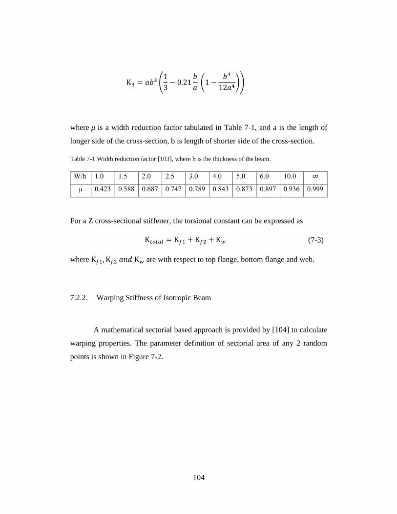
104

K3 = 𝑎𝑏3 (1

3− 0.21

𝑏

𝑎 (1 −

𝑏4

12𝑎4))

where 𝜇 is a width reduction factor tabulated in Table 7-1, and a is the length of

longer side of the cross-section, b is length of shorter side of the cross-section.

Table 7-1 Width reduction factor [103], where h is the thickness of the beam.

W/h 1.0 1.5 2.0 2.5 3.0 4.0 5.0 6.0 10.0 ∞

μ 0.423 0.588 0.687 0.747 0.789 0.843 0.873 0.897 0.936 0.999

For a Z cross-sectional stiffener, the torsional constant can be expressed as

K𝑡𝑜𝑡𝑎𝑙 = K𝑓1 + K𝑓2 + K𝑤 (7-3)

where K𝑓1, K𝑓2 𝑎𝑛𝑑 K𝑤 are with respect to top flange, bottom flange and web.

7.2.2. Warping Stiffness of Isotropic Beam

A mathematical sectorial based approach is provided by [104] to calculate

warping properties. The parameter definition of sectorial area of any 2 random

points is shown in Figure 7-2.

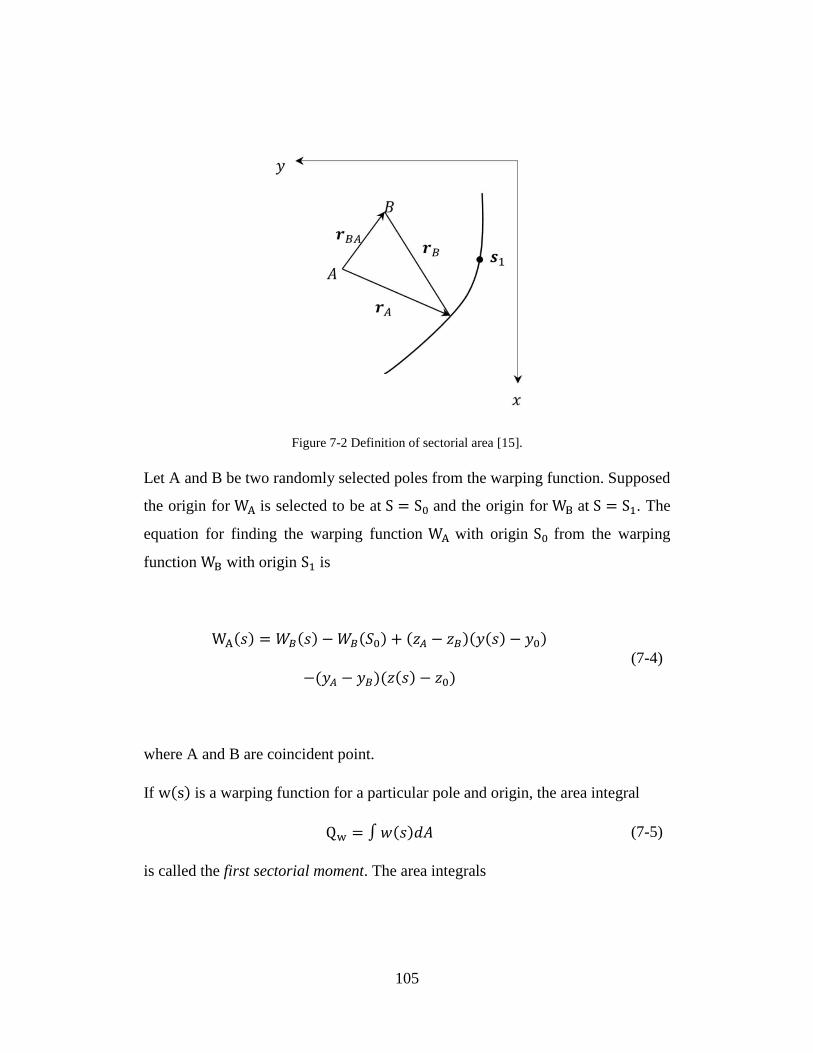
105

Figure 7-2 Definition of sectorial area [15].

Let A and B be two randomly selected poles from the warping function. Supposed

the origin for WA is selected to be at S = S0 and the origin for WB at S = S1. The

equation for finding the warping function WA with origin S0 from the warping

function WB with origin S1 is

WA(𝑠) = 𝑊𝐵(𝑠) −𝑊𝐵(𝑆0) + (𝑧𝐴 − 𝑧𝐵)(𝑦(𝑠) − 𝑦0)

−(𝑦𝐴 − 𝑦𝐵)(𝑧(𝑠) − 𝑧0) (7-4)

where A and B are coincident point.

If w(s) is a warping function for a particular pole and origin, the area integral

Qw = ∫𝑤(𝑠)𝑑𝐴 (7-5)

is called the first sectorial moment. The area integrals

106

𝐼𝑦𝑤 = ∫ 𝑦(𝑠)𝑤(𝑠)𝑑𝐴

𝐼𝑧𝑤 = ∫ 𝑧(𝑠)𝑤(𝑠)𝑑𝐴

(7-6)

are known as the sectorial products of area. Moreover, the definition of the first,

second, and product moments of area can be expressed as

𝑄𝑦 = ∫ 𝑧𝑑𝐴

𝑄𝑧 = ∫ 𝑦𝑑𝐴

𝐼𝑦 = ∫ 𝑧2𝑑𝐴

𝐼𝑧 = ∫ 𝑦2𝑑𝐴

𝐼𝑦𝑧 = ∫ 𝑦𝑧𝑑𝐴

(7-7)

The important concept here is when those sectorial products of area are both equal

zero, the pole is called principal pole, or shear center. By integrating both sides of

the results over the cross-section area and multiplying both sides, we can obtain

𝐼𝑦𝑤𝐴 = 𝐼𝑦𝑤𝐵 − 𝑤𝐵(𝑆0)𝑄𝑍 + (𝑧𝐴 − 𝑧𝐵)(𝐼𝑧 − 𝑦0𝑄𝑧)

− (𝑦𝐴 − 𝑦𝐵)(𝐼𝑦𝑧 − 𝑧0𝑄𝑧) (7-8)

Since the origin of the y, z axis is the centroid C of the cross section, the first

moments 𝑄𝑧 and 𝑄𝑦 are both zero. For the conditions for A to be a principal pole

𝐼𝑦𝑤𝐴 = 𝐼𝑧𝑤𝐴 = 0 (7-9)

Therefore,

𝑦𝐴 = 𝑦𝐵 +𝐼𝑧𝑤𝐵𝐼𝑧 − 𝐼𝑦𝑤𝐵𝐼𝑦𝑧

𝐼𝑦𝐼𝑧 − 𝐼𝑦𝑧2 (7-10)

107

𝑧𝐴 = 𝑧𝐵 +𝐼𝑧𝑤𝐵𝐼𝑦𝑧 − 𝐼𝑦𝑤𝐵𝐼𝑦

𝐼𝑦𝐼𝑧 − 𝐼𝑦𝑧2

If, for a given pole A, there is a sectorial origin 𝑠0 such that

𝑄𝑤𝐴 = ∫𝑤𝐴(𝑠) 𝑑𝐴 = 0 (7-11)

The point 𝑠0 is termed as a principal origin. Let B be a pole coincident with A but

with a known origin 𝑠1,

𝑤𝐴(𝑠) = 𝑤𝐵(𝑠) − 𝑤𝐵(𝑠0) (7-12)

Hence, for a given cross section, it is possible to find a pole A and an origin s0 so

that 𝑄𝑤𝐴, 𝐼𝑦𝑤𝐴, and 𝐼𝑧𝑊𝐴 are zero.

7.2.3. Warping Stiffness of Isotropic Z-Stiffener

Considering an isotropic beam with Z cross-section as shown in Figure 7-3,

the dimensions are:

𝑏1 = 𝑊𝑓1 −ℎ𝑤2 𝑏2 = 𝑊𝑓𝑤 −

ℎ𝑤2 ℎ = 𝑊𝑤 +

ℎ𝑓1

2+ℎ𝑓2

2 (7-13)

The centroid C is at a horizontal distance 𝑑 and a vertical distance e from the

intersection O of the lower flange and the web

𝑑 = ��𝑐 −ℎ𝑤2 𝑒 = ��𝑐 −

ℎ𝑓2

2 (7-14)

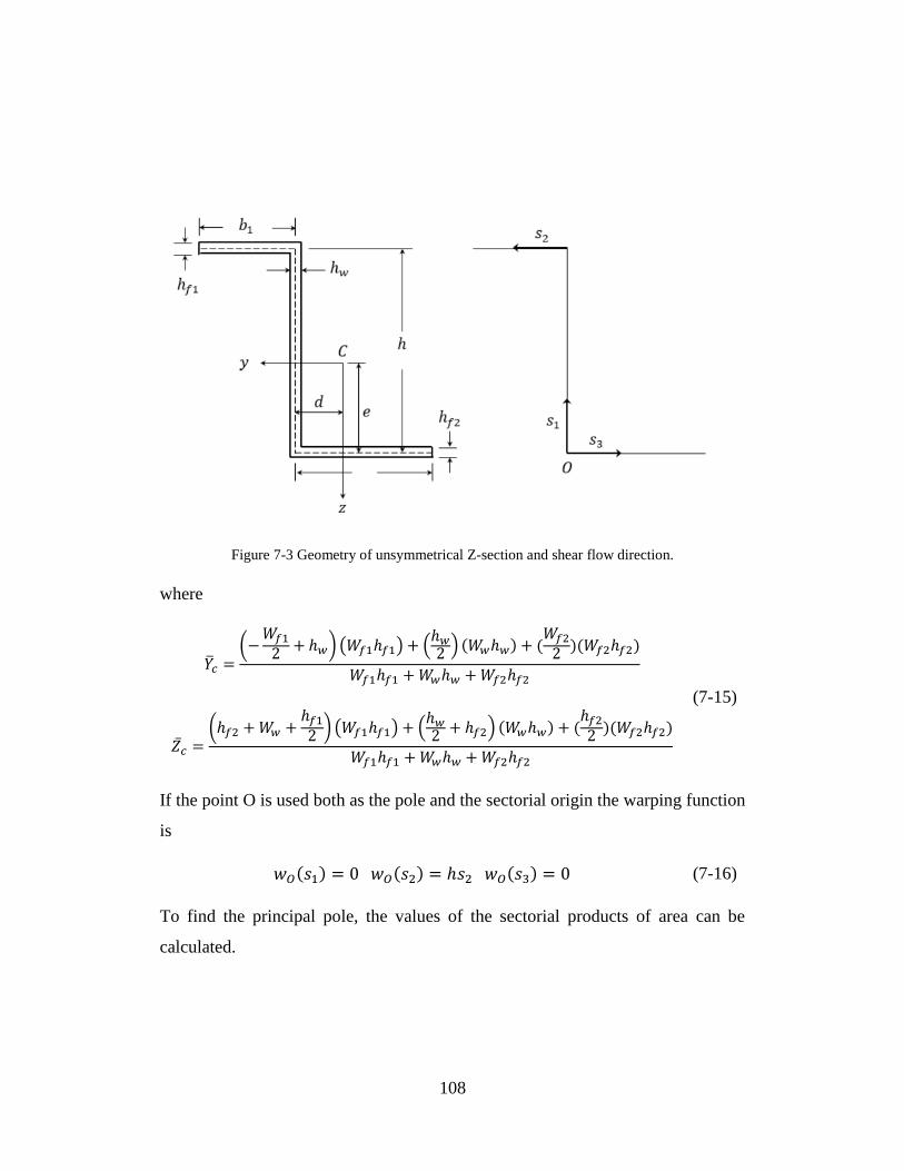
108

Figure 7-3 Geometry of unsymmetrical Z-section and shear flow direction.

where

��𝑐 =(−

𝑊𝑓12+ ℎ𝑤) (𝑊𝑓1ℎ𝑓1) + (

ℎ𝑤2) (𝑊𝑤ℎ𝑤) + (

𝑊𝑓22)(𝑊𝑓2ℎ𝑓2)

𝑊𝑓1ℎ𝑓1 +𝑊𝑤ℎ𝑤 +𝑊𝑓2ℎ𝑓2

��𝑐 =(ℎ𝑓2 +𝑊𝑤 +

ℎ𝑓12 ) (𝑊𝑓1ℎ𝑓1) + (

ℎ𝑤2 + ℎ𝑓2) (𝑊𝑤ℎ𝑤) + (

ℎ𝑓22 )(𝑊𝑓2ℎ𝑓2)

𝑊𝑓1ℎ𝑓1 +𝑊𝑤ℎ𝑤 +𝑊𝑓2ℎ𝑓2

(7-15)

If the point O is used both as the pole and the sectorial origin the warping function

is

𝑤𝑂(𝑠1) = 0 𝑤𝑂(𝑠2) = ℎ𝑠2 𝑤𝑂(𝑠3) = 0 (7-16)

To find the principal pole, the values of the sectorial products of area can be

calculated.

109

𝐼𝑦𝑤𝑂 = ∫𝑦𝑤𝑂𝑑𝐴𝑦 = ∫(𝑑 + 𝑠2)𝑤𝑂(𝑠2)ℎ𝑓1𝑑𝑠2

𝑏1

0

𝐼𝑧𝑤𝑂 = ∫𝑧𝑤𝑂𝑑𝐴𝑦 = ∫ (−ℎ + 𝑒)𝑤𝑂(𝑠2)ℎ𝑓1𝑑𝑠2

𝑏1

0

(7-17)

The principal pole A or shear center can be expressed as

𝑌𝑠𝑜 = 𝑦𝐴 = 𝑦𝑂 −𝐼𝑧𝑤𝐵𝐼𝑧 − 𝐼𝑦𝑤𝐵𝐼𝑦𝑧


𝑍𝑠𝑜 = 𝑧𝐴 = 𝑧𝑂 −𝐼𝑧𝑤𝐵𝐼𝑦𝑧 − 𝐼𝑦𝑤𝐵𝐼𝑦


(7-18)

The warping function with principal pole A and origin O is

𝑤𝐴(𝑠1) = −(𝑦𝐴 − 𝑦𝑂)𝑠1

𝑤𝐴(𝑠2) = −(𝑦𝐴 − 𝑦𝑂)ℎ + (ℎ − 𝑧𝐴)𝑠2

𝑤𝐴(𝑠3) = 𝑧𝐴𝑠3

(7-19)

The first sectorial area moment is

𝑄𝑤𝐴 = ∫𝑤𝐴(𝑠1)ℎ𝑤𝑑𝑠1 +

ℎ

0

∫ 𝑤𝐴(𝑠2)ℎ𝑓1𝑑𝑠2 +

𝑏1

0

∫ 𝑤𝐴(𝑠3)ℎ𝑓2𝑑𝑠3

𝑏2

0

(7-20)

The condition for 𝑠0 to be a principal origin is

𝑤𝐴(𝑠0) =𝑄𝑤𝐴𝐴

(7-21)

where 𝐴 = 𝑊𝑓1ℎ𝑓1 +𝑊𝑤ℎ𝑤 +𝑊𝑓2ℎ𝑓2

The principal warping functions

110

𝑤(𝑠1) = 𝑤𝐴(𝑠1) − 𝑤𝐴(𝑠0)

𝑤(𝑠2) = 𝑤𝐴(𝑠2) − 𝑤𝐴(𝑠0)

𝑤(𝑠3) = 𝑤𝐴(𝑠3) − 𝑤𝐴(𝑠0)

(7-22)

Therefore, the warping constant 𝐼𝑤 (or Γ ) can be computed as

𝐼𝑤 = ∫𝑤(𝑠1)2ℎ𝑤𝑑𝑠1 +

ℎ

0

∫ 𝑤(𝑠2)2ℎ𝑓1𝑑𝑠2 +

𝑏1

0

∫ 𝑤(𝑠3)2ℎ𝑓2𝑑𝑠3 =

𝑏2

0

Γ (7-23)

The torque due to warping is

Tw = −𝐸Γ𝑑3𝜃

𝑑𝑥3 (7-24)

where E = Axial stiffness, Γ = Warping constant, EΓ = Warping stiffness.

The total torque will be resisted by St Venant’s shearing stresses and warping

torsion. The derivation is well documented in [100].

T = Tsv + 𝑇𝑤 = 𝐺𝐾𝑑𝜃

𝑑𝑥− 𝐸Γ

𝑑3𝜃

𝑑𝑥3 (7-25)

Rearranging and writing 𝜇2 =𝐺𝐾

𝐸𝛤 to solve

𝑑𝜃

𝑑𝑥, we have

𝑑3𝜃

𝑑𝑥3− 𝜇2

𝑑𝜃

𝑑𝑥= −𝜇2

𝑇

𝐺𝐾 (7-26)

Applying boundary conditions with

1. When x = 0, the slope of beam equals zero.

2. When x = L, the bending moment is zero.

111

𝑑𝜃

𝑑𝑥=

𝑇

𝐺𝐾(1 −

cosh 𝜇(𝐿 − 𝑥)

cosh 𝜇𝐿) (7-27)

Thus, θ can be solved.

𝜃𝑤𝑎𝑟𝑝 =𝑇

𝐺𝐾(𝑥 +

sinh𝜇(𝐿 − 𝑥)

𝜇 cosh 𝜇𝐿−

sinh𝜇𝐿

𝜇 cosh 𝜇𝐿) (7-28)

When x = L,

𝜃𝑤𝑎𝑟𝑝 =𝑇𝐿

𝐺𝐾(1 −

tanh𝜇𝐿

𝜇𝐿) (7-29)

Considering only free torsion case,

θsv =𝑇𝐿

𝐺𝐾 (7-30)

7-3 Constitutive Equation of Composite Z-Stiffener

7-3.1 Constitutive Equation of Laminated Composite Beam under Torsion

The foundation of beam analysis is based upon the one-dimensional moment-

curvature relationship along the longitudinal axis of the beam under bending and upon

the torque-twist angle relationship along the center axis of twist of the cross-section

for torsion. This approach for laminated composite beams is similar with the approach

used in isotropic beams. However, evaluation of the sectional properties is different.

These properties are not only dependent of the geometry of the cross-section but also

composite material properties and their stacking sequence. Composite material is

inherent with two-dimensional property. Hence, an equivalent one-dimensional

112

property of composite beam is needed. The equivalent one-dimensional property is

dependent of the structural response of the deformed beam and the structural response

of the beam is dependent on the ratio of the width to height of the beam cross-section.

Beam with general, wide, and narrow sections under axial and bending are discussed

in Chapter 4-2. The axial and bending stiffness under general, wide, and narrow

sections are shown in Eqs. (4-7), (4-9), and (4-15).

For the case of torsion, no axial strains, 𝜀𝑥0 and 𝜀𝑦

0 as well as 𝐾𝑥 exist. However,

a non-zero 𝑀𝑥 is induced for the laminate under torsion. The narrow laminate

constitutive equation subjected to torsion is given as

[𝑁𝑥𝑦𝑀𝑥𝑦

] = [𝐴𝑇∗ 𝐵𝑇

∗

𝐵𝑇∗ 𝐷𝑇

∗] [𝛾𝑥𝑦0

𝜅𝑥𝑦] 𝑎𝑛𝑑 [

𝐴𝑇∗ 𝐵𝑇

∗


∗] = [𝑎𝑇∗ 𝑏𝑇

∗

𝑏𝑇∗ 𝑑𝑇

∗ ]−1

(7-31)

where

𝑎𝑇∗ = (𝑎66 −

𝑏612

𝑑11) ; 𝑏𝑇

∗ = (𝑏66 − 𝑏61𝑑16𝑑11

) ; 𝑑𝑇∗ = (𝑑66 −

𝑑162

𝑑11) (7-32)

It should be noted that the properties with a subscript, T refer to laminate under

torsion. In general, b61 and b16 are not the same. The shear center, Zsc measuring

from the mid-plane of the laminate can be obtained by setting shear strain with

absence of 𝑁𝑥𝑦 .

𝑧𝑠𝑐 = −𝛾𝑥𝑦0

𝜅𝑥𝑦= −

𝑏𝑇∗

𝑑𝑇∗ (7-33)

The torsional stiffness of the laminate at the shear center, Zsc can be obtained by using

the parallel theorem as

𝐷𝑇𝑠𝑐∗ = 𝐷𝑇

∗ − 2𝑧𝑠𝑐𝐵𝑇∗ + 𝑧𝑠𝑐

2 𝐴𝑇∗ (7-34)

113

Like beam of isotropic material, an edge correction factor is needed to

accommodate the zero shear boundary condition. The torsional stiffness, 𝐺𝐾 is

modified by a correction factor, μ as shown below:

𝐺𝐾 = 4𝑏 𝜇 𝐷𝑇𝑠𝑐∗ (7-35)

In this analysis, the correction factor used for isotropic material as listed in [105] is

adopted. For a finite rectangular cross-section of the beam, the twist curvature is twice

of the rate of the twisting angle, 𝜙 and the torque, T is twice of total twisting moment

of the laminate, b*𝑀𝑥𝑦 where b is the width of laminate.

𝜙 = 𝑇

4𝑏 𝐷𝑇𝑠𝑐∗ (7-36)

7-3.2 Shear Center

The shear center for composite beam depends on the geometry of the cross-

section, material properties, and the stack sequence. It is an important sectional

property because the bending and torsion are uncoupled at the shear center.

Twisting will be induced if only torque is applied and vice versa. The axial and

bending stiffness for composite Z-stiffener are provided [106, 107] as shown below

��𝑥 = [𝑤𝑓1(𝐴1,𝑓1∗ ) + 𝑤𝑓2(𝐴1,𝑓2

∗ ) + 𝑤𝑤(𝐴𝑤∗ )] (7-37)

114

��𝑧 = {[𝐴1,𝑓1∗ [𝑦𝑐,𝑓1

2 𝑤𝑓1 + (𝑤𝑓13

12) ]]

+ [𝐴1,𝑓2∗ [𝑦𝑐,𝑓2

2 𝑤𝑓2 + (𝑤𝑓23

12) ]]

+ [𝐷𝑤∗ 𝑤𝑤 + 𝐴𝑤

∗ 𝑦𝑐,𝑤2 𝑤𝑤 + 2 𝐵𝑤

∗ 𝑦𝑐,𝑤 𝑤𝑤]}

��𝑦𝑧 = {(𝐴1,𝑓1∗ 𝑤𝑓1 𝑦𝑐,𝑓1 𝑧𝑐,𝑓1 + 𝐵1,𝑓1

∗ 𝑤𝑓1 𝑦𝑐,𝑓1)

+ (𝐴1,𝑓2 ∗ 𝑤𝑓2 𝑦𝑐,𝑓2 𝑧𝑐,𝑓2 + 𝐵1,𝑓2

∗ 𝑤𝑓2 𝑦𝑐,𝑓2)

+ (𝐵𝑤∗ 𝑤𝑤 𝑧𝑐,𝑤 + 𝐴𝑤

∗ 𝑤𝑤 𝑧𝑐,𝑤 𝑦𝑐,𝑤)}

��𝑦 = [𝑤𝑓1 𝐷1,𝑓1∗ +𝑤𝑓1 𝐴1,𝑓1

∗ 𝑧𝑐,𝑓12 + 2 𝑤𝑓1 𝐵1,𝑓1

∗ 𝑧𝑐,𝑓1 + 𝑤𝑓2 𝐷1,𝑓2∗

+𝑤𝑓2 𝐴1,𝑓2∗ 𝑧𝑐,𝑓2

2 + 2 𝑤𝑓2 𝐵1,𝑓2 ∗ 𝑧𝑐,𝑓2

+ 𝐴1,𝑤∗ [𝑧𝑐,𝑤

2 𝑤𝑤 + (𝑤𝑤3

12) ]]

Curvatures for a composite Z-stiffener under bending can be expressed as

𝐾𝑦 =��𝑦

��𝑦��𝑧 − ��𝑦𝑧2 𝐾𝑧 =

��𝑧

��𝑦��𝑧 − ��𝑦𝑧2 𝐾𝑦𝑧 =

��𝑦𝑧

��𝑦��𝑧 − ��𝑦𝑧2 (7-38)

Curvature at centroid can be written as

𝐾𝑦𝑐 = ��𝑦𝐾𝑧 − ��𝑧𝐾𝑦𝑧 𝐾𝑧

𝑐 = ��𝑧𝐾𝑦 − ��𝑧𝐾𝑦𝑧 (7-39)

115

Figure 7-4 Geometry of composite Z-stiffener and load components.

Distances from top flange, lower flange and web to the origin and loading

schematic is shown in Figure 7-4. Strain of the top flange can be expressed as

𝜀𝑥𝑓10 = 𝜀𝑥

0 + 𝑦𝐾𝑧𝑐 + 𝑧𝐾𝑦

𝑐 (7-40)

where

𝜀𝑥0 =

𝑁𝑥

��𝑥 (7-41)

Relationship between applied moment/force and induced shearing force along y

and z-direction can be expressed as

𝜕𝑁𝑥𝜕𝑥

= 0 𝜕��𝑧

𝜕𝑥= 𝑉𝑦

𝜕��𝑦

𝜕𝑥= 𝑉𝑧 (7-42)

Substituting Eqs. (7-41) into (7-42), the following equation can be obtained.

𝜕𝑁𝑥𝑓1𝜕𝑥

= 𝐴1𝑓1∗ [𝑦(𝑉𝑦𝐾𝑦 − 𝑉𝑧𝐾𝑦𝑧) − 𝑧(𝑉𝑧𝐾𝑧 − 𝑉𝑦𝐾𝑦𝑧)] (7-43)

116

If there is no load applied in the axial direction, the equilibrium equation can be

expressed as

𝜕𝑞

𝜕𝑠+𝜕𝑁𝑥𝜕𝑥

= 0 (7-44)

where q = Shear flow, s = The flow direction, Nx = Total force in x-direction (lb/in).

Rearranging Eqs. (7-44), we can obtained:

𝜕𝑞𝑓1

𝜕𝑠1= −

𝜕𝑁𝑥𝑓1𝜕𝑥

= −𝐴1𝑓1∗ [𝑦(𝑉𝑦𝐾𝑦 − 𝑉𝑧𝐾𝑦𝑧) − 𝑧(𝑉𝑧𝐾𝑧 − 𝑉𝑦𝐾𝑦𝑧)] (7-45)

The shear flow on the top flange after integration can be written as

𝑞𝑓1 = ∫ −𝐴1𝑓1∗ [𝑦(𝑉𝑦𝐾𝑦 − 𝑉𝑧𝐾𝑦𝑧) − 𝑧(𝑉𝑧𝐾𝑧 − 𝑉𝑦𝐾𝑦𝑧)]𝑑𝑠1

𝑠1

0

(7-46)

Due to unsymmetrical cross-section, both shear force 𝑉𝑦 and 𝑉𝑧 has necessary to be

applied. The shear flow on top flange due to 𝑉𝑦 and 𝑉𝑧 applied at the shear center

are

𝑞𝑓1𝑦= −(𝑉𝑦𝐾𝑦)∫ 𝐴1𝑓1

∗ 𝑦𝑑𝑠1 − (−𝑉𝑦𝐾𝑦𝑧)∫ 𝐴1𝑓1∗ 𝑧𝑑𝑠1

𝑠1

0

𝑠1

0

𝑞𝑓1𝑧= −(𝑉𝑧𝐾𝑦𝑧)∫ 𝐴1𝑓1

∗ 𝑦𝑑𝑠1 − (𝑉𝑧𝐾𝑧)∫ 𝐴1𝑓1∗ 𝑧𝑑𝑠1

𝑠1

0

𝑠1

0

(7-47)

where y = −Wf1 + ℎ𝑤 − ��𝑐 + 𝑠1 and z = 𝑧𝑐𝑓1.

The shear forces acting on the top flange are introduced as

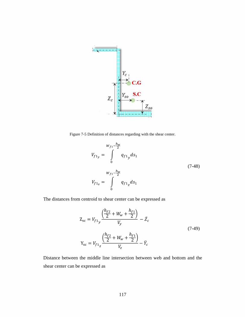
117

Figure 7-5 Definition of distances regarding with the shear center.

𝑉𝑓1𝑦 = ∫ 𝑞𝑓1𝑦𝑑𝑠1

𝑊𝑓1−ℎ𝑤2

0

𝑉𝑓1𝑧 = ∫ 𝑞𝑓1𝑧𝑑𝑠1


0

(7-48)

The distances from centroid to shear center can be expressed as

Zsc = 𝑉𝑓1𝑦

(ℎ𝑓22 +𝑊𝑤 +

ℎ𝑓12 )

𝑉𝑦 − ��𝑐

Ysc = 𝑉𝑓1𝑧

(ℎ𝑓22 +𝑊𝑤 +

ℎ𝑓12 )

𝑉𝑧− ��𝑐

(7-49)

Distance between the middle line intersection between web and bottom and the

shear center can be expressed as

118

Zso = 𝑍𝑠𝑐 + ��𝑐

Yso = 𝑌𝑠𝑐 + ��𝑐 (7-50)

7-3.3 Torsional Stiffness of Composite Z-Stiffener

Based on CLT, the relationship for a thin rectangular cross-section can be

shown as

[ 𝜀𝑥0

𝜀𝑦0

𝛾𝑥𝑦0

𝑘𝑥𝑘𝑦𝑘𝑥𝑦]

=

[ 𝑎11 𝑎12 𝑎16 𝑏11 𝑏12 𝑏16𝑎12 𝑎22 𝑎26 𝑏21 𝑏22 𝑏26𝑎16 𝑎26 𝑎66 𝑏61 𝑏62 𝑏66𝑏11 𝑏21 𝑏61 𝑑11 𝑑12 𝑑16𝑏12 𝑏22 𝑏62 𝑑12 𝑑22 𝑑26𝑏16 𝑏26 𝑏66 𝑑16 𝑑26 𝑑66]

[ 𝑁𝑥𝑁𝑦𝑁𝑥𝑦𝑀𝑥

𝑀𝑦

𝑀𝑥𝑦]

(7-51)

At shear center, bending and twisting are decoupled. On the other hand, for

torsional center or we called center of twist, it does not move when the member

twist. That is, twisting and shearing are decoupled at torsional center. However, if

beam subjects only to torsion, it is surprise that the center of twist is identical as

shear center. That is, the bending-torsion-shear are decoupled. Thus, for a thin

rectangular composite section under a torque, Eqs. (7-51) will be reduced to

[

𝛾𝑥𝑦0

𝑘𝑥𝑘𝑥𝑦

] = [

𝑎66 𝑏61 𝑏66𝑏61 𝑑11 𝑑16𝑏66 𝑑16 𝑑66

] [

𝑁𝑥𝑦𝑀𝑥

𝑀𝑥𝑦

] (7-52)

If pure torque subjected to the shear center is considered, the curvature in x-

direction is equal to zero.

𝑘𝑥 = 𝑏61𝑁𝑥𝑦 + 𝑑11𝑀𝑥 + 𝑑16𝑀𝑥𝑦 = 0 (7-53)

119

Solving for Eqs. (7-52),

𝑀𝑥 = −(𝑏61𝑑11

𝑁𝑥𝑦 +𝑑16𝑑11

𝑀𝑥𝑦) (7-54)

Substituting Eqs. (7-54) to (7-52), the mid-plane shear strain and curvature are

obtained.

γxy0 = (𝑎66 −

𝑏612

𝑑11)𝑁𝑥𝑦 + (𝑏66 −

𝑏61𝑑16𝑑11

)𝑀𝑥𝑦

𝑘𝑥𝑦 = (𝑏66 −𝑏61𝑑16𝑑11

)𝑁𝑥𝑦 + (𝑑66 −𝑑162

𝑑11)𝑀𝑥𝑦

(7-55)

The constitutive equation for a beam under pure torsion can be expressed as

[𝛾𝑥𝑦0

𝑘𝑥𝑦] = [

𝑎𝑇∗ 𝑏𝑇

∗


∗ ] [𝑁𝑥𝑦𝑀𝑥𝑦

] (7-56)

where

𝑎𝑇∗ = (𝑎66 −

𝑏612

𝑑11) 𝑏𝑇

∗ = (𝑏66 −𝑏61𝑑16𝑑11

) 𝑑𝑇∗ = (𝑑66 −

𝑑162

𝑑11) (7-57)

Under pure torsion assumption, the mid-plane shear strain can curvature are

simplified as

γxy0 = 𝑏𝑇

∗𝑀𝑥𝑦

kxy = 𝑑𝑇∗𝑀𝑥𝑦

(7-58)

It should be noted that the shear strain at the shear center is equal to zero.

γxy = 0 = 𝛾𝑥𝑦0 + 𝜌𝑠𝑐𝑘𝑥𝑦 (7-59)

120

Solving for Eqs. (7-59),

ρsc = −𝛾𝑥𝑦0

𝑘𝑥𝑦= −

𝑏𝑇∗

𝑑𝑇∗ (7-60)

The effective stiffness are

[𝐴𝑇∗ 𝐵𝑇

∗


∗] = [𝑎𝑇∗ 𝑏𝑇

∗


∗ ]−1

(7-61)

Stiffness should all shift to the location of center of twist by a distance ρsc

AT𝑠𝑐∗ = 𝐴𝑇

∗

BT𝑠𝑐∗ = 𝐵𝑇

∗ − 𝜌𝑠𝑐𝐴𝑇∗

DTsc∗ = 𝐷𝑇

∗ − 2𝜌𝑠𝑐𝐵𝑇∗ + 𝜌𝑠𝑐

2 𝐴𝑇∗

(7-62)

Due to twisting and bending decoupled at the shear center, BTsc∗ = 0. Definition for

curvature and moment in x-y direction can be written as

𝑘𝑥𝑦 = −2𝜕2𝑤

𝜕𝑥𝜕𝑦= −2

𝜕𝜕𝑤𝜕𝑦

𝜕𝑥= −2

𝜕𝜃𝑇𝜕𝑥

= −2𝜙𝑇

Mxy = −𝑇

2𝑏

(7-63)

where 𝜙𝑇 = rate of twist = 𝜕𝜃𝑇

𝜕𝑥, 𝑇 is the applied torque and 𝑏 is the width of the

laminate. Substituting Eqs. (7-63) to (7-62), the rate of twist is

𝜙𝑇 =𝑇

4𝑏𝐷𝑇𝑠𝑐∗ (7-64)

Therefore, for a rectangular cross-section, the torsion stiffness is

121

𝐺𝐾 = 4𝑏𝐷𝑇𝑠𝑐∗ (7-65)

The torsion stiffness for a composite rectangular cross-section depends on material

properties, stack sequence, and ply orientation of the laminate. Considering Z-

section geometry, since it belongs open thin wall sections, the torsion stiffness can

be approximated added together, which is similar to isotropic cases. Three different

method discussed in [108] are implemented in order to compute overall torsional

stiffness for a composite Z-stiffener as shown below.

𝐺𝐾1 = 𝐺𝐾𝑓1 + 𝐺𝐾𝑓2 + 𝐺𝐾𝑤 = 4𝑤𝑓1𝐷𝑇𝑠𝑐𝑓1∗ + 4𝑤𝑓2𝐷𝑇𝑠𝑐𝑓2

∗ + 4𝑤𝑤𝐷𝑇𝑠𝑐𝑤∗

𝐺𝐾2 = 𝐺𝐾𝑓1 + 𝐺𝐾𝑓2 + 𝐺𝐾𝑤 =4𝑤𝑓1

𝑑66𝑓1+4𝑤𝑓2

𝑑66𝑓2+4𝑤𝑤𝑑66𝑤

𝐺𝐾3 = 𝐺𝐾𝑓1 + 𝐺𝐾𝑓2 + 𝐺𝐾𝑤 = 𝜇𝑓14𝑤𝑓1𝐷𝑇𝑠𝑐𝑓1∗ + 𝜇𝑓24𝑤𝑓2𝐷𝑇𝑠𝑐𝑓2

∗ + 𝜇𝑤4𝑤𝑤𝐷𝑇𝑠𝑐𝑤∗

(7-66)

where 𝐺𝐾𝑓1 = Torsion stiffness of top flange. 𝐺𝐾𝑓2 = Torsion stiffness of bottom

flange. 𝐺𝐾𝑤 = Torsion stiffness of web.

7-3.4 Warping Stiffness of Composite Z-Stiffener

The warping stiffness of an isotropic beam is function of modulus E and

thickness h [109]. The 𝐸ℎ is related to the axial force (per unit length) inside the

wall can be shown as follow,

𝑁x = ℎ𝜎𝑥 = 𝐸ℎεx0 (7-67)

For a beam with orthotropic layup,

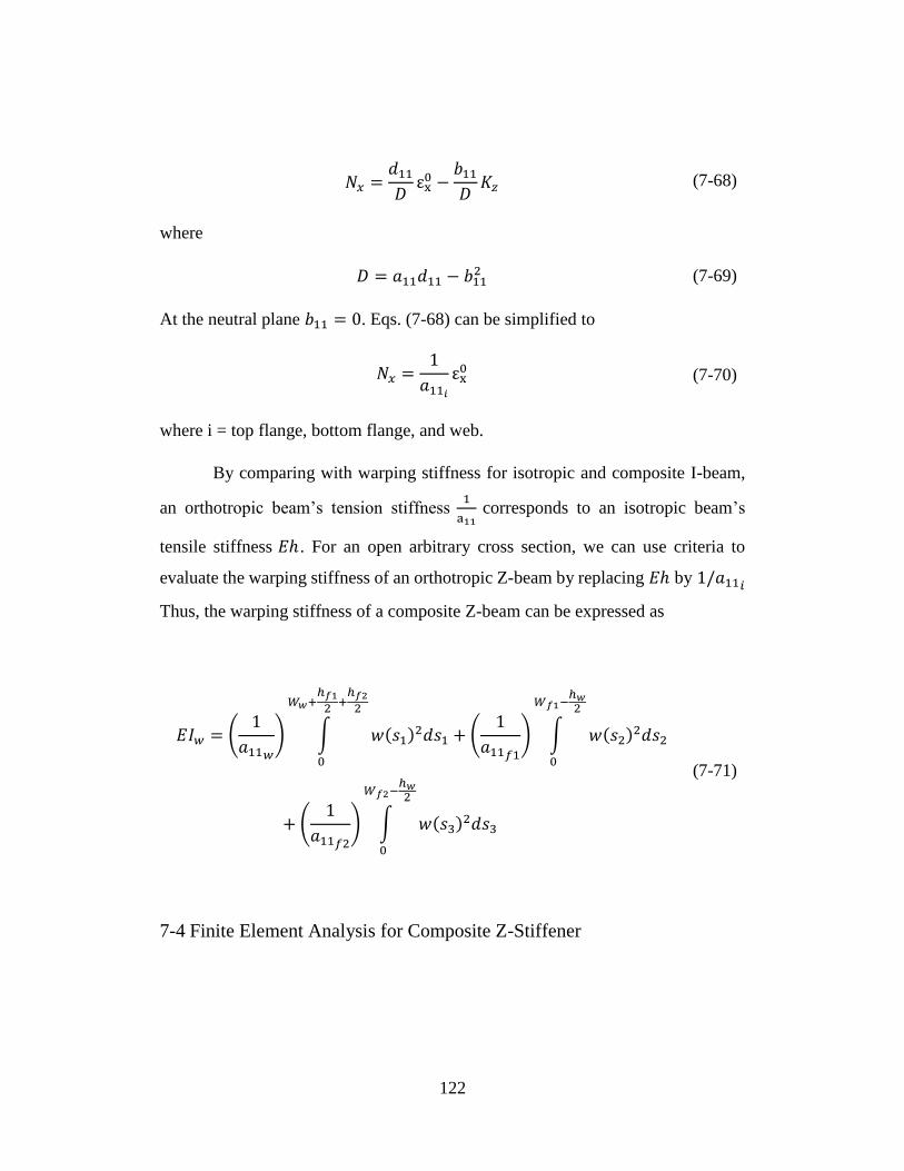
122

𝑁𝑥 =𝑑11𝐷εx0 −

𝑏11𝐷𝐾𝑧 (7-68)

where

𝐷 = 𝑎11𝑑11 − 𝑏112 (7-69)

At the neutral plane 𝑏11 = 0. Eqs. (7-68) can be simplified to

𝑁𝑥 =1

𝑎11𝑖εx0 (7-70)

where i = top flange, bottom flange, and web.

By comparing with warping stiffness for isotropic and composite I-beam,

an orthotropic beam’s tension stiffness 1

a11 corresponds to an isotropic beam’s

tensile stiffness 𝐸ℎ . For an open arbitrary cross section, we can use criteria to

evaluate the warping stiffness of an orthotropic Z-beam by replacing 𝐸ℎ by 1/𝑎11𝑖

Thus, the warping stiffness of a composite Z-beam can be expressed as

𝐸𝐼𝑤 = (1

𝑎11𝑤) ∫ 𝑤(𝑠1)

2𝑑𝑠1 + (1

𝑎11𝑓1) ∫ 𝑤(𝑠2)

2𝑑𝑠2


0

𝑊𝑤+ℎ𝑓12+ℎ𝑓22

0

+ (1

𝑎11𝑓2) ∫ 𝑤(𝑠3)

2𝑑𝑠3


0

(7-71)

7-4 Finite Element Analysis for Composite Z-Stiffener

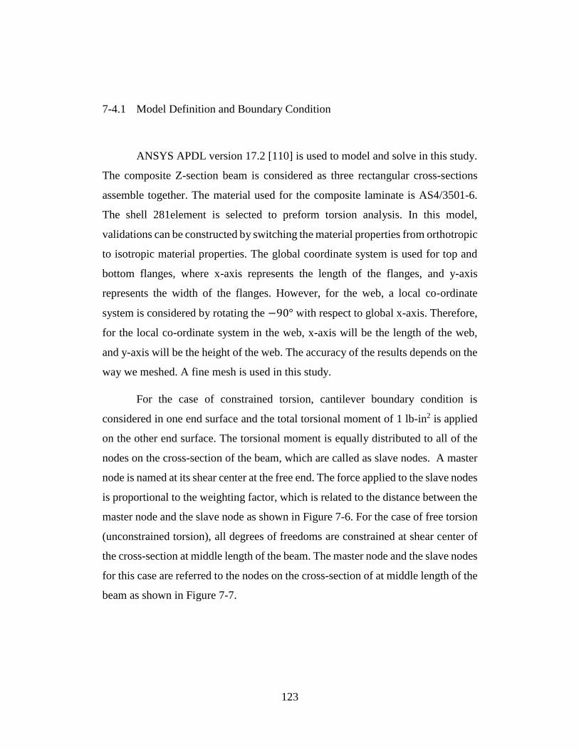
123

7-4.1 Model Definition and Boundary Condition

ANSYS APDL version 17.2 [110] is used to model and solve in this study.

The composite Z-section beam is considered as three rectangular cross-sections

assemble together. The material used for the composite laminate is AS4/3501-6.

The shell 281element is selected to preform torsion analysis. In this model,

validations can be constructed by switching the material properties from orthotropic

to isotropic material properties. The global coordinate system is used for top and

bottom flanges, where x-axis represents the length of the flanges, and y-axis

represents the width of the flanges. However, for the web, a local co-ordinate

system is considered by rotating the −90° with respect to global x-axis. Therefore,

for the local co-ordinate system in the web, x-axis will be the length of the web,

and y-axis will be the height of the web. The accuracy of the results depends on the

way we meshed. A fine mesh is used in this study.

For the case of constrained torsion, cantilever boundary condition is

considered in one end surface and the total torsional moment of 1 lb-in2 is applied

on the other end surface. The torsional moment is equally distributed to all of the

nodes on the cross-section of the beam, which are called as slave nodes. A master

node is named at its shear center at the free end. The force applied to the slave nodes

is proportional to the weighting factor, which is related to the distance between the

master node and the slave node as shown in Figure 7-6. For the case of free torsion

(unconstrained torsion), all degrees of freedoms are constrained at shear center of

the cross-section at middle length of the beam. The master node and the slave nodes

for this case are referred to the nodes on the cross-section of at middle length of the

beam as shown in Figure 7-7.

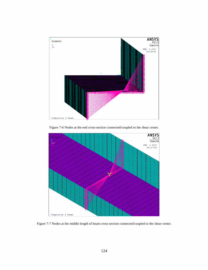
124

Figure 7-6 Nodes at the end cross-section connected/coupled to the shear center.

Figure 7-7 Nodes at the middle length of beam cross-section connected/coupled to the shear center.

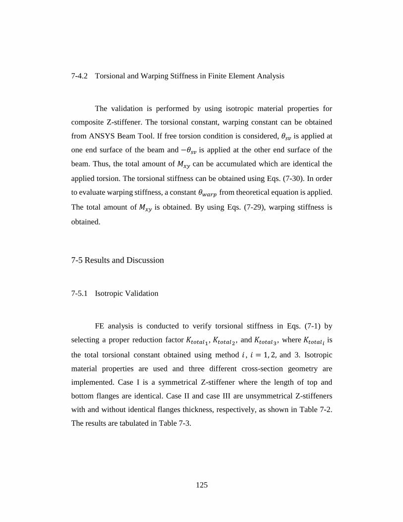
125

7-4.2 Torsional and Warping Stiffness in Finite Element Analysis

The validation is performed by using isotropic material properties for

composite Z-stiffener. The torsional constant, warping constant can be obtained

from ANSYS Beam Tool. If free torsion condition is considered, 𝜃𝑠𝑣 is applied at

one end surface of the beam and −𝜃𝑠𝑣 is applied at the other end surface of the

beam. Thus, the total amount of 𝑀𝑥𝑦 can be accumulated which are identical the

applied torsion. The torsional stiffness can be obtained using Eqs. (7-30). In order

to evaluate warping stiffness, a constant 𝜃𝑤𝑎𝑟𝑝 from theoretical equation is applied.

The total amount of 𝑀𝑥𝑦 is obtained. By using Eqs. (7-29), warping stiffness is

obtained.


7-5.1 Isotropic Validation

FE analysis is conducted to verify torsional stiffness in Eqs. (7-1) by

selecting a proper reduction factor 𝐾𝑡𝑜𝑡𝑎𝑙1, 𝐾𝑡𝑜𝑡𝑎𝑙2, and 𝐾𝑡𝑜𝑡𝑎𝑙3, where 𝐾𝑡𝑜𝑡𝑎𝑙𝑖 is

the total torsional constant obtained using method 𝑖 , 𝑖 = 1, 2, and 3. Isotropic

material properties are used and three different cross-section geometry are

implemented. Case I is a symmetrical Z-stiffener where the length of top and

bottom flanges are identical. Case II and case III are unsymmetrical Z-stiffeners

with and without identical flanges thickness, respectively, as shown in Table 7-2.

The results are tabulated in Table 7-3.

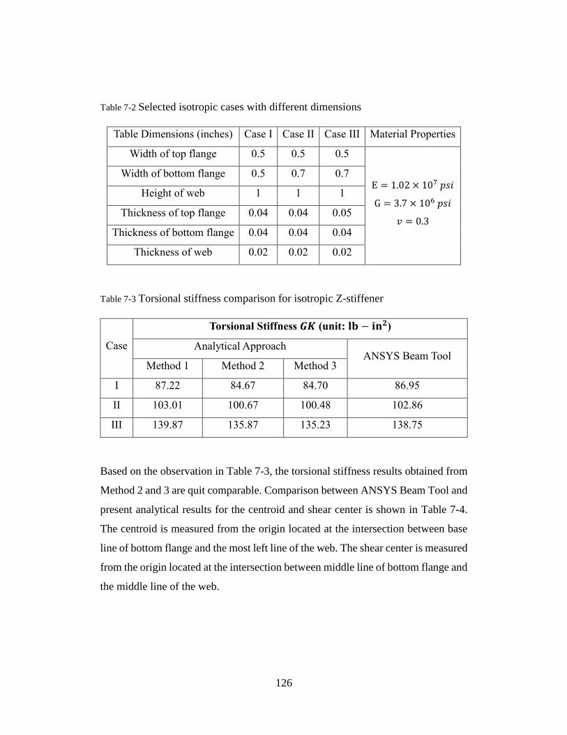
126

Table 7-2 Selected isotropic cases with different dimensions

Table Dimensions (inches) Case I Case II Case III Material Properties

Width of top flange 0.5 0.5 0.5

E = 1.02 × 107 𝑝𝑠𝑖

G = 3.7 × 106 𝑝𝑠𝑖

𝑣 = 0.3

Width of bottom flange 0.5 0.7 0.7

Height of web 1 1 1

Thickness of top flange 0.04 0.04 0.05

Thickness of bottom flange 0.04 0.04 0.04

Thickness of web 0.02 0.02 0.02

Table 7-3 Torsional stiffness comparison for isotropic Z-stiffener

Case

Torsional Stiffness 𝑮𝑲 (unit: 𝐥𝐛 − 𝐢𝐧𝟐)

Analytical Approach ANSYS Beam Tool

Method 1 Method 2 Method 3

I 87.22 84.67 84.70 86.95

II 103.01 100.67 100.48 102.86

III 139.87 135.87 135.23 138.75

Based on the observation in Table 7-3, the torsional stiffness results obtained from

Method 2 and 3 are quit comparable. Comparison between ANSYS Beam Tool and

present analytical results for the centroid and shear center is shown in Table 7-4.

The centroid is measured from the origin located at the intersection between base

line of bottom flange and the most left line of the web. The shear center is measured

from the origin located at the intersection between middle line of bottom flange and

the middle line of the web.

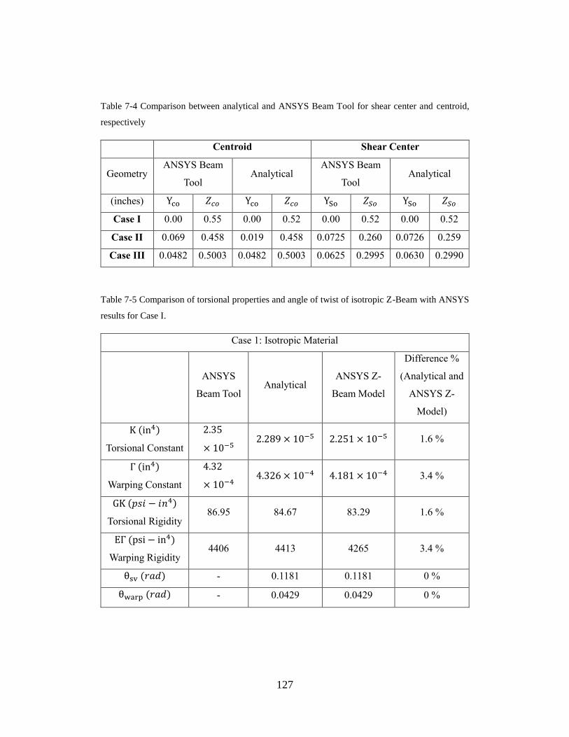
127

Table 7-4 Comparison between analytical and ANSYS Beam Tool for shear center and centroid,

respectively

Centroid Shear Center

Geometry ANSYS Beam

Tool Analytical

ANSYS Beam

Tool Analytical

(inches) Yco 𝑍𝑐𝑜 Yco 𝑍𝑐𝑜 YSo 𝑍𝑆𝑜 YSo 𝑍𝑆𝑜

Case I 0.00 0.55 0.00 0.52 0.00 0.52 0.00 0.52

Case II 0.069 0.458 0.019 0.458 0.0725 0.260 0.0726 0.259

Case III 0.0482 0.5003 0.0482 0.5003 0.0625 0.2995 0.0630 0.2990

Table 7-5 Comparison of torsional properties and angle of twist of isotropic Z-Beam with ANSYS

results for Case I.

Case 1: Isotropic Material

ANSYS

Beam Tool Analytical

ANSYS Z-

Beam Model

Difference %

(Analytical and

ANSYS Z-

Model)

K (in4)

Torsional Constant

2.35

× 10−5 2.289 × 10−5 2.251 × 10−5 1.6 %

Γ (in4)

Warping Constant

4.32

× 10−4 4.326 × 10−4 4.181 × 10−4 3.4 %

GK (𝑝𝑠𝑖 − 𝑖𝑛4)

Torsional Rigidity 86.95 84.67 83.29 1.6 %

EΓ (psi − in4)

Warping Rigidity 4406 4413 4265 3.4 %

θsv (𝑟𝑎𝑑) - 0.1181 0.1181 0 %

θwarp (𝑟𝑎𝑑) - 0.0429 0.0429 0 %

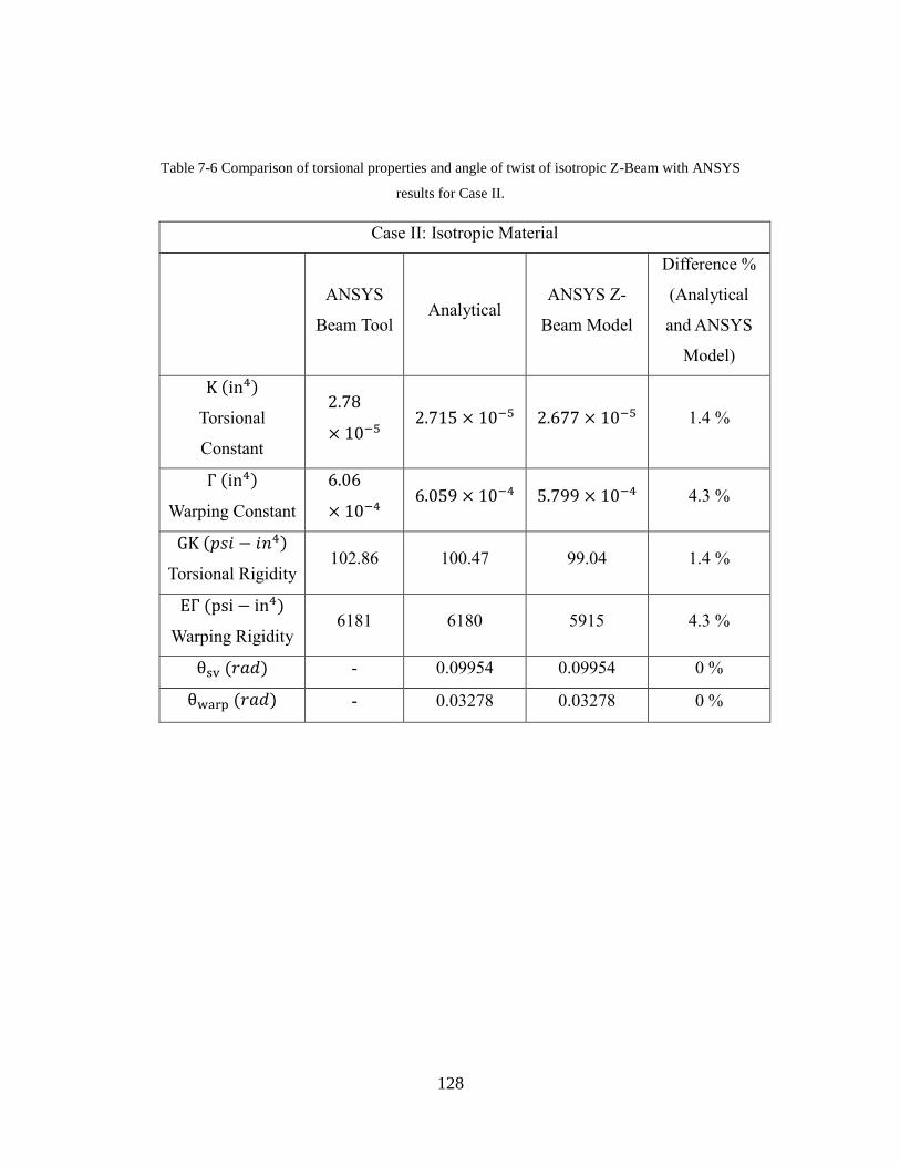
128


results for Case II.

Case II: Isotropic Material

ANSYS


ANSYS Z-

Beam Model

Difference %

(Analytical

and ANSYS

Model)

K (in4)

Torsional

Constant

2.78

× 10−5 2.715 × 10−5 2.677 × 10−5 1.4 %

Γ (in4)

Warping Constant

6.06

× 10−4 6.059 × 10−4 5.799 × 10−4 4.3 %


Torsional Rigidity 102.86 100.47 99.04 1.4 %

EΓ (psi − in4)


θsv (𝑟𝑎𝑑) - 0.09954 0.09954 0 %

θwarp (𝑟𝑎𝑑) - 0.03278 0.03278 0 %

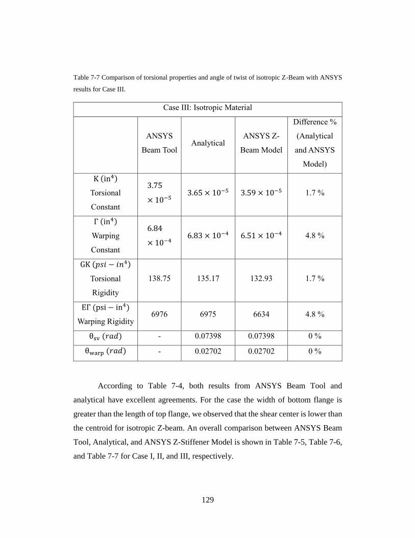
129


results for Case III.

Case III: Isotropic Material

ANSYS


ANSYS Z-

Beam Model

Difference %

(Analytical

and ANSYS

Model)

K (in4)

Torsional

Constant

3.75

× 10−5 3.65 × 10−5 3.59 × 10−5 1.7 %

Γ (in4)

Warping

Constant

6.84

× 10−4 6.83 × 10−4 6.51 × 10−4 4.8 %


Torsional

Rigidity

138.75 135.17 132.93 1.7 %

EΓ (psi − in4)


θsv (𝑟𝑎𝑑) - 0.07398 0.07398 0 %

θwarp (𝑟𝑎𝑑) - 0.02702 0.02702 0 %

According to Table 7-4, both results from ANSYS Beam Tool and

analytical have excellent agreements. For the case the width of bottom flange is

greater than the length of top flange, we observed that the shear center is lower than

the centroid for isotropic Z-beam. An overall comparison between ANSYS Beam

Tool, Analytical, and ANSYS Z-Stiffener Model is shown in Table 7-5, Table 7-6,

and Table 7-7 for Case I, II, and III, respectively.

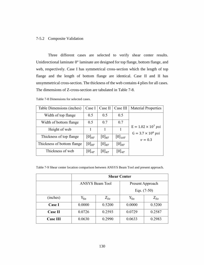
130

7-5.2 Composite Validation

Three different cases are selected to verify shear center results.

Unidirectional laminate 0° laminate are designed for top flange, bottom flange, and

web, respectively. Case I has symmetrical cross-section which the length of top

flange and the length of bottom flange are identical. Case II and II has

unsymmetrical cross-section. The thickness of the web contains 4 plies for all cases.

The dimensions of Z-cross-section are tabulated in Table 7-8.

Table 7-8 Dimensions for selected cases.

Table Dimensions (inches) Case I Case II Case III Material Properties

Width of top flange 0.5 0.5 0.5

E = 1.02 × 107 𝑝𝑠𝑖

G = 3.7 × 106 𝑝𝑠𝑖

𝑣 = 0.3

Width of bottom flange 0.5 0.7 0.7

Height of web 1 1 1

Thickness of top flange [0]8𝑇 [0]8𝑇 [0]10𝑇

Thickness of bottom flange [0]8𝑇 [0]8𝑇 [0]8𝑇

Thickness of web [0]4𝑇 [0]4𝑇 [0]4𝑇

Table 7-9 Shear center location comparison between ANSYS Beam Tool and present approach.

Shear Center

ANSYS Beam Tool Present Approach

Eqs. (7-50)

(inches) YSo 𝑍𝑆𝑜 YSo 𝑍𝑆𝑜

Case I 0.0000 0.5200 0.0000 0.5200

Case II 0.0726 0.2593 0.0729 0.2587

Case III 0.0630 0.2990 0.0633 0.2983

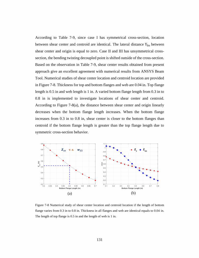
131

According to Table 7-9, since case I has symmetrical cross-section, location

between shear center and centroid are identical. The lateral distance YSo between

shear center and origin is equal to zero. Case II and III has unsymmetrical cross-

section, the bending twisting decoupled point is shifted outside of the cross-section.

Based on the observation in Table 7-9, shear center results obtained from present

approach give an excellent agreement with numerical results from ANSYS Beam

Tool. Numerical studies of shear center location and centroid location are provided

in Figure 7-8. Thickness for top and bottom flanges and web are 0.04 in. Top flange

length is 0.5 in and web length is 1 in. A varied bottom flange length from 0.3 in to

0.8 in is implemented to investigate locations of shear center and centroid.

According to Figure 7-8(a), the distance between shear center and origin linearly

decreases when the bottom flange length increases. When the bottom flange

increases from 0.3 in to 0.8 in, shear center is closer to the bottom flanges than

centroid if the bottom flange length is greater than the top flange length due to

symmetric cross-section behavior.

Figure 7-8 Numerical study of shear center location and centroid location if the length of bottom

flange varies from 0.3 in to 0.8 in. Thickness in all flanges and web are identical equals to 0.04 in.

The length of top flange is 0.5 in and the length of web is 1 in.

𝒁𝒔𝒐 𝐯. 𝐬. 𝒘𝒇𝟐

(a) (b)

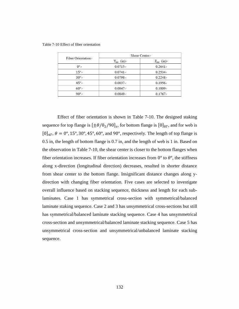
132

Table 7-10 Effect of fiber orientation

Effect of fiber orientation is shown in Table 7-10. The designed staking

sequence for top flange is [±𝜃/02/90]𝑠, for bottom flange is [0]8𝑇, and for web is

[0]4𝑇, 𝜃 = 0°, 15°, 30°, 45°, 60°, and 90°, respectively. The length of top flange is

0.5 in, the length of bottom flange is 0.7 in, and the length of web is 1 in. Based on

the observation in Table 7-10, the shear center is closer to the bottom flanges when

fiber orientation increases. If fiber orientation increases from 0° to 𝜃°, the stiffness

along x-direction (longitudinal direction) decreases, resulted in shorter distance

from shear center to the bottom flange. Insignificant distance changes along y-

direction with changing fiber orientation. Five cases are selected to investigate

overall influence based on stacking sequence, thickness and length for each sub-

laminates. Case 1 has symmetrical cross-section with symmetrical/balanced

laminate staking sequence. Case 2 and 3 has unsymmetrical cross-sections but still

has symmetrical/balanced laminate stacking sequence. Case 4 has unsymmetrical

cross-section and unsymmetrical/balanced laminate stacking sequence. Case 5 has

unsymmetrical cross-section and unsymmetrical/unbalanced laminate stacking

sequence.

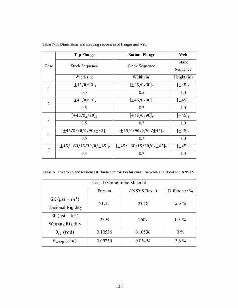
133

Table 7-11 Dimensions and stacking sequences of flanges and web.

Case

Top Flange Bottom Flange Web

Stack Sequence Stack Sequence Stack

Sequence

Width (in) Width (in) Height (in)

1 [±45/0/90]𝑠 [±45/0/90]𝑠 [±45]𝑠

0.5 0.5 1.0

2 [±45/0/90]𝑠 [±45/0/90]𝑠 [±45]𝑠

0.5 0.7 1.0

3 [±45/02/90]𝑠 [±45/0/90]𝑠 [±45]𝑠

0.5 0.7 1.0

4 [±45/0/90/0/90/±45]𝑇 [±45/0/90/0/90/±45]𝑇 [±45]𝑠

0.5 0.7 1.0

5 [±45/−60/15/30/0/±45]𝑇 [±45/−60/15/30/0/±45]𝑇 [±45]𝑠

0.5 0.7 1.0

Table 7-12 Warping and torsional stiffness comparison for case 1 between analytical and ANSYS.

Case 1: Orthotropic Material

Present ANSYS Result Difference %


Torsional Rigidity 91.18 88.85 2.6 %

EΓ (psi − in4)

Warping Rigidity 2598 2607 0.3 %

θsv (𝑟𝑎𝑑) 0.10536 0.10536 0 %

θwarp (𝑟𝑎𝑑) 0.05259 0.05454 3.6 %

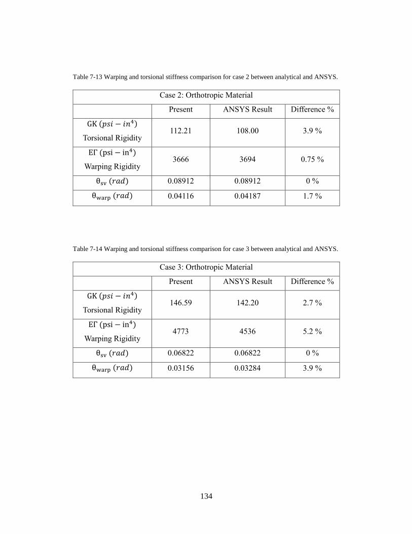
134






EΓ (psi − in4)


θsv (𝑟𝑎𝑑) 0.08912 0.08912 0 %

θwarp (𝑟𝑎𝑑) 0.04116 0.04187 1.7 %






EΓ (psi − in4)


θsv (𝑟𝑎𝑑) 0.06822 0.06822 0 %

θwarp (𝑟𝑎𝑑) 0.03156 0.03284 3.9 %

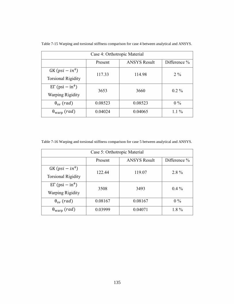
135





Torsional Rigidity 117.33 114.98 2 %

EΓ (psi − in4)


θsv (𝑟𝑎𝑑) 0.08523 0.08523 0 %

θwarp (𝑟𝑎𝑑) 0.04024 0.04065 1.1 %






EΓ (psi − in4)


θsv (𝑟𝑎𝑑) 0.08167 0.08167 0 %

θwarp (𝑟𝑎𝑑) 0.03999 0.04071 1.8 %

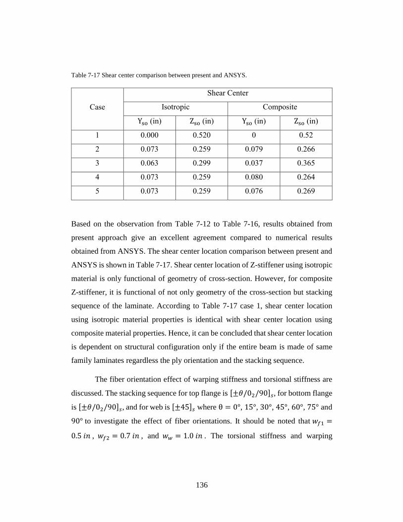
136

Table 7-17 Shear center comparison between present and ANSYS.

Case

Shear Center

Isotropic Composite

Yso (in) Zso (in) Yso (in) Zso (in)

1 0.000 0.520 0 0.52

2 0.073 0.259 0.079 0.266

3 0.063 0.299 0.037 0.365

4 0.073 0.259 0.080 0.264

5 0.073 0.259 0.076 0.269

Based on the observation from Table 7-12 to Table 7-16, results obtained from

present approach give an excellent agreement compared to numerical results

obtained from ANSYS. The shear center location comparison between present and

ANSYS is shown in Table 7-17. Shear center location of Z-stiffener using isotropic

material is only functional of geometry of cross-section. However, for composite

Z-stiffener, it is functional of not only geometry of the cross-section but stacking

sequence of the laminate. According to Table 7-17 case 1, shear center location

using isotropic material properties is identical with shear center location using

composite material properties. Hence, it can be concluded that shear center location

is dependent on structural configuration only if the entire beam is made of same

family laminates regardless the ply orientation and the stacking sequence.

The fiber orientation effect of warping stiffness and torsional stiffness are

discussed. The stacking sequence for top flange is [±𝜃/02/90]𝑠, for bottom flange

is [±𝜃/02/90]𝑠, and for web is [±45]𝑠 where θ = 0°, 15°, 30°, 45°, 60°, 75° and

90° to investigate the effect of fiber orientations. It should be noted that 𝑤𝑓1 =

0.5 𝑖𝑛 , 𝑤𝑓2 = 0.7 𝑖𝑛 , and 𝑤𝑤 = 1.0 𝑖𝑛 . The torsional stiffness and warping

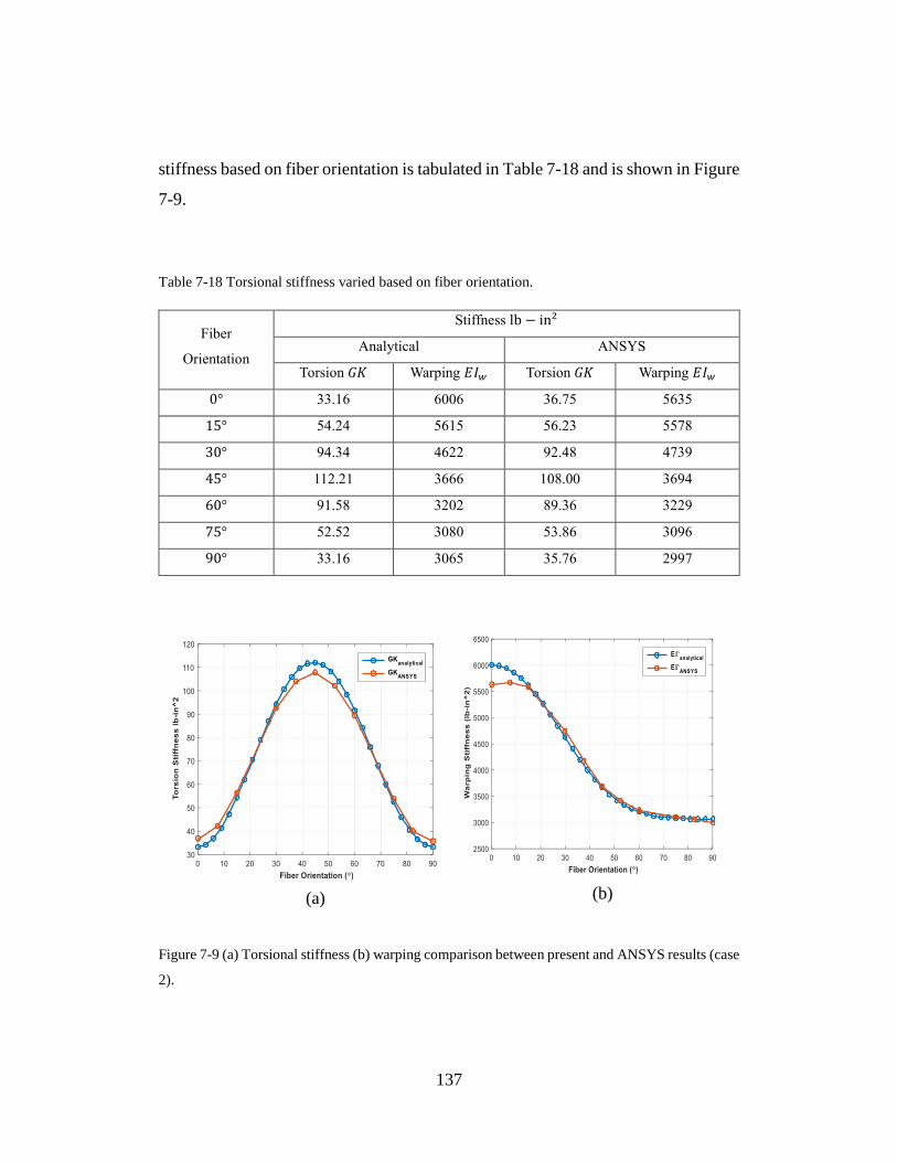
137

stiffness based on fiber orientation is tabulated in Table 7-18 and is shown in Figure

7-9.

Table 7-18 Torsional stiffness varied based on fiber orientation.

Fiber

Orientation

Stiffness lb − in2

Analytical ANSYS

Torsion 𝐺𝐾 Warping 𝐸𝐼𝑤 Torsion 𝐺𝐾 Warping 𝐸𝐼𝑤

0° 33.16 6006 36.75 5635

15° 54.24 5615 56.23 5578

30° 94.34 4622 92.48 4739

45° 112.21 3666 108.00 3694

60° 91.58 3202 89.36 3229

75° 52.52 3080 53.86 3096

90° 33.16 3065 35.76 2997

Figure 7-9 (a) Torsional stiffness (b) warping comparison between present and ANSYS results (case

2).

(a) (b)

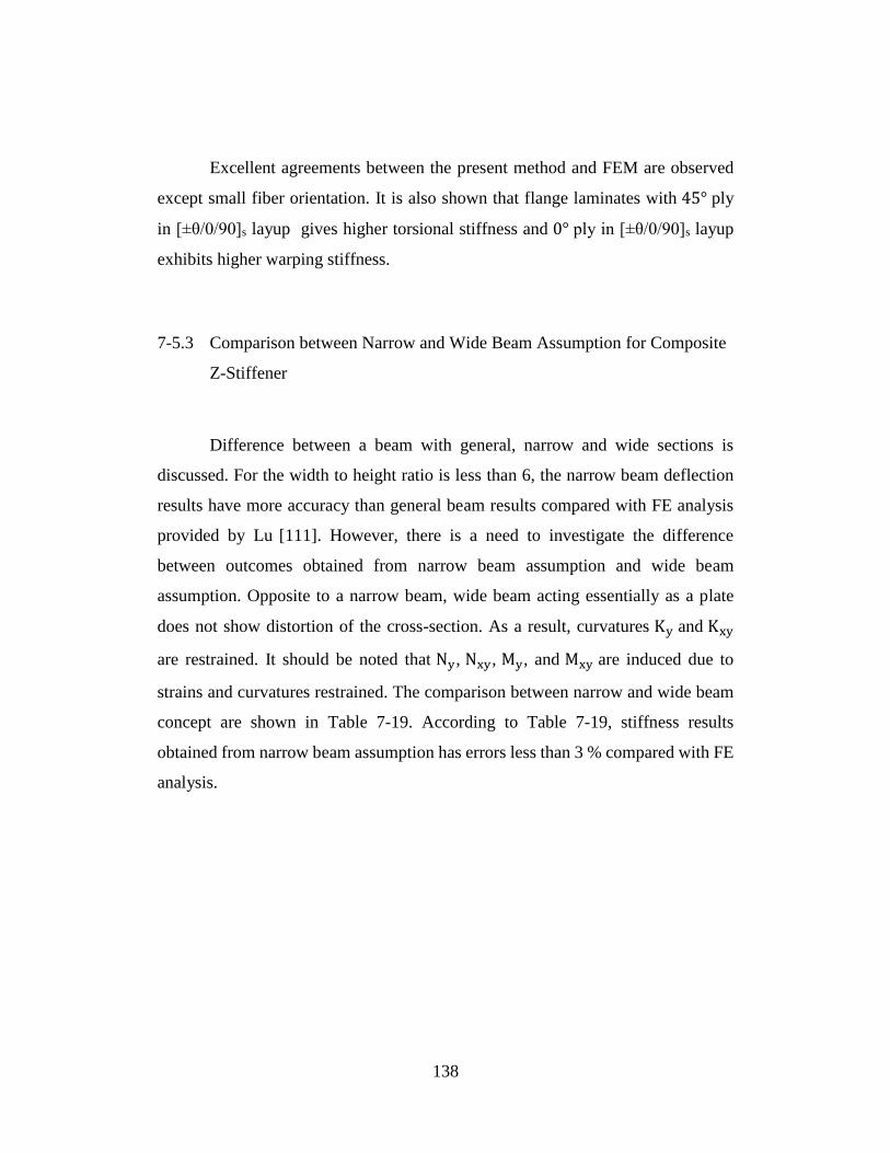
138

Excellent agreements between the present method and FEM are observed

except small fiber orientation. It is also shown that flange laminates with 45° ply

in [±θ/0/90]s layup gives higher torsional stiffness and 0° ply in [±θ/0/90]s layup

exhibits higher warping stiffness.

7-5.3 Comparison between Narrow and Wide Beam Assumption for Composite

Z-Stiffener

Difference between a beam with general, narrow and wide sections is

discussed. For the width to height ratio is less than 6, the narrow beam deflection

results have more accuracy than general beam results compared with FE analysis

provided by Lu [111]. However, there is a need to investigate the difference

between outcomes obtained from narrow beam assumption and wide beam

assumption. Opposite to a narrow beam, wide beam acting essentially as a plate

does not show distortion of the cross-section. As a result, curvatures Ky and Kxy

are restrained. It should be noted that Ny, Nxy, My, and Mxy are induced due to

strains and curvatures restrained. The comparison between narrow and wide beam

concept are shown in Table 7-19. According to Table 7-19, stiffness results

obtained from narrow beam assumption has errors less than 3 % compared with FE

analysis.

139

Table 7-19 Comparison between narrow and wide beam assumptions.

Case 2 Case 3

Ax Ky𝑐 Kz

𝑐 Ax Ky𝑐 Kz

𝑐

Narrow 4.436E5 2.951E-06 3.771E-06 5.787E5 2.248E-6 2.730E-6

Wide 5.397E5 2.395E-6 3.052E-6 6.758E5 1.909E-6 2.329E-6

ANSYS 4.424E5 2.953E-06 3.777E-06 5.779E5 2.233E-6 2.728E-6

% Diff.

(Narrow) -0.25 0.07 0.16 -0.13 0.67 0.07

% Diff.

(Wide) 21.93 18.89 19.16 -17.12 -14.51 -14.63

Case 4 Case 5

Ax Ky𝑐 Kz

𝑐 Ax Ky𝑐 Kz

𝑐

Narrow 4.430E5 2.953E-6 3.774E-6 4.222E5 3.002E-6 3.805E-6

Wide 5.398E5 2.395E-6 3.050E-6 5.973E5 2.173E-6 2.772E-6

ANSYS 4.423E5 2.955E-6 3.746E-6 4.223E5 3.11E-6 3.875E-6

% Diff.

(Narrow) -0.19 0.07 -0.75 0.03 2.99 1.29

% Diff.

(Wide) 22.04 -18.95 -18.58 41.44 -30.13 -28.46

140

7-6 Conclusion for Composite Z-Stiffener

An analytical method is developed to calculate the sectional properties and ply

stresses of the z-beam under torsion. The sectional properties include shear center,

equivalent torsional and wrapping stiffness of a laminated composite beam with Z

cross-section. The developed expression takes into consideration of the structural

deformation characteristics of composite beam with narrow section. The difference

between beams with narrow and wide sections is studied. The sectional properties

and the ply stresses of flanges and web laminates are computed for composite Z-

stiffener torsional loads. The present results give excellent agreement with the

results obtained from ANSYS™. A parametric study of shear center and centroid

with various layup sequences ranging from the combination of

symmetric/unsymmetrical and balanced/unbalanced laminates was performed

using the present solution. It is found that the sectional properties of a composite

Z-stiffener structure are dependent on the laminate material properties and stacking

sequence besides its structural configuration if the flange and web laminates are

made of different family of laminates. However, the sectional properties are

dependent on structural configuration only if the entire beam is made of same

family laminates regardless the ply orientation and the stacking sequence. It is

concluded that the present approach for analyzing a composite z-stiffener is a viable

and efficient method for composite z-stiffener design.

141

CONCLUSION AND FURTURE WORK

This research fundamentally provides the analytical development of simple

closed-form solutions for accurately predicting key structural characteristics such

as equivalent axial stiffness, bending stiffness, and ply-stress variations for a

composite curved beam under bending. A closed-form analytical solution is

developed for analyzing laminated composite beam with and without curvature and

fiber waviness, respectively. The explicit expression for evaluating axial and

bending stiffness are formulated based on consideration of structural deformation

of beam with narrow cross-section. Closed-form solutions are also provided to

predict overall structural stiffness behavior for a composite curved beam with in-

plane fiber waviness or out-of-plane fiber waviness. FE analysis is conducted for

verifying the analytical results. The present stiffness and stress variation results

have excellent agreement with numerical results obtained from ABAQUS.

Significant stiffness reduction is observed when fiber waviness ratio 𝑅 varies from

0 to 0.3. A specific ratio when 𝑅 = 0.72 is introduced, where Young’s modulus

along the x-direction and y-direction are identical. If the ratio is over 0.72, the

stiffness along the y-direction is greater than the stiffness along the x-direction

because larger portion of fiber now align in the y-direction, which contributes the

most stiffness for the structure. In curved laminate stage, both axial stiffness and

bending stiffness decrease for a composite curved beam with fiber waviness. It is

more pronounced for axial stiffness since significant axial stiffness reduction is

observed when the amplitude of fiber waviness increases. However, fiber waviness

has less impact on the bending stiffness of plies which is affected by fiber wariness

near the middle axis of the composite curved beam. The maximum radial stress for

142

a composite curved beam with fiber waviness under bending is discussed. The

maximum radial stress increases about 25 % when a fiber waviness is present and

the fiber waviness amplitude is equal to 10 % of the total thickness of the beam. It

is concluded that the present approach can provide an efficient method for

analyzing laminated composite curved beam with in-plane and out-of-plane fiber

waviness.

The analytical closed-form solution is developed to calculate the total strain

ERR for a composite curved beam under bending. The crack is allowed to locate in

any arbitrary interface and location in the present research. Symmetrical model and

unsymmetrical model are developed to capture the total strain ERR. Linear scaling

parameters are provided to predict the total strain ERR in the present approach to

aim the void where inaccurate strain ERR is obtained for a given small crack. FE

analysis is implemented to verify analytical results, VCCT techniques is

implemented and the total strain ERR in the crack tips are studied. If the total crack

angle is 5.4°, a bending moment 8.356 N-m can be applied on the composite curved

beam without failure. However, if the total crack angle 32.4° is considered, only a

moment 3.287 N-m can be applied on the composite curved beam without failure.

Significant failure loading reduction is observed when crack angle increases

from 5.4° to 32.4°. The total strain ERR also varies with the radius of crack. The

strain ERR reaches to maximum at the location where maximum σr is observed of

a prefect composite curved beam under bending. The effect of crack hoop location

is also investigated. If crack locates near θh = 40°, the applied moment is 38 %

higher than the crack locates at θh = 0°. In conclusion, the present successfully

fills the void where previous authors couldn’t predict accurately for a composite

curved beam with a small crack. Moreover, this study allows the crack can be

located in any interface and hoop locations, which provides a feasible way to

efficiently analyze composite curved beam with a crack and the total strain ERR

143

results can be predicted accurately for the type of curved beam where Rm/𝑡 ratio is

less than 3.5.

The last chapter discussed of composite Z-stiffener which is the application of

composite curved beam. An analytical method is developed to calculate the

sectional properties and ply stresses of the z-beam under torsion. The sectional

properties include shear center, equivalent torsional and wrapping stiffness of a

laminated composite beam with Z cross-section. Narrow beam assumption has to

be applied if a thin-walled structures is considered. The equivalent stiffness

comparison between NB and WB assumptions is provided. The present results give

excellent agreement with the results obtained from ANSYS™. A parametric study

of shear center and centroid with various layup sequences ranging from the

combination of symmetric/unsymmetrical and balanced/unbalanced laminates was

performed using the present solution. It is found that the sectional properties of a

composite Z-stiffener structure are dependent on the laminate material properties

and stacking sequence besides its structural configuration if the flange and web

laminates are made of different family of laminates. However, the sectional

properties are dependent on structural configuration only if the entire beam is made

of same family laminates regardless the ply orientation and the stacking sequence.

In conclusion, the present research provides an overall study of composite

curved beam with fiber waviness and delamination under bending. Equivalent

stiffness closed-form solutions to calculate axial and bending stiffness are provided

for a composite curved beam with/without curvature and fiber waviness,

respectively. The closed-form analytical solution for analyzing composite curved

beam with delamination is developed. Torsional stiffness and warping stiffness are

also studied for a composite Z-stiffener. It is concluded that the present approach

is a viable and efficient method for composite beam design with and without fiber

144

waviness and delamination. The research initiated in this study provides further

motivation to the following topics:

• Shear stress prediction for a composite curved beam with an out-of-plane

fiber waviness.

• 3-D numerical modeling of investigation in composite curved beam with a

void using VCCT.

• Stress concentration factor of voids and stress intensity factor of cracks

inside the composite curved beam under bending.

• Extend present approach to study “Spring-in” and “Spring-out” effects

where data is provided from [112].

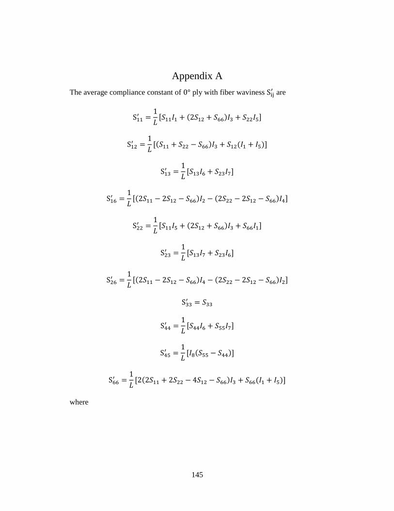
145

Appendix A

The average compliance constant of 0° ply with fiber waviness Sij′ are

S11′ =

1

𝐿[𝑆11𝐼1 + (2𝑆12 + 𝑆66)𝐼3 + 𝑆22𝐼5]

S12′ =

1

𝐿[(𝑆11 + 𝑆22 − 𝑆66)𝐼3 + 𝑆12(𝐼1 + 𝐼5)]

S13′ =

1

𝐿[𝑆13𝐼6 + 𝑆23𝐼7]

S16′ =

1

𝐿[(2𝑆11 − 2𝑆12 − 𝑆66)𝐼2 − (2𝑆22 − 2𝑆12 − 𝑆66)𝐼4]

S22′ =

1

𝐿[𝑆11𝐼5 + (2𝑆12 + 𝑆66)𝐼3 + 𝑆66𝐼1]

S23′ =

1

𝐿[𝑆13𝐼7 + 𝑆23𝐼6]

S26′ =

1

𝐿[(2𝑆11 − 2𝑆12 − 𝑆66)𝐼4 − (2𝑆22 − 2𝑆12 − 𝑆66)𝐼2]

S33′ = 𝑆33

S44′ =

1

𝐿[𝑆44𝐼6 + 𝑆55𝐼7]

S45′ =

1

𝐿[𝐼8(𝑆55 − 𝑆44)]

S66′ =

1

𝐿[2(2𝑆11 + 2𝑆22 − 4𝑆12 − 𝑆66)𝐼3 + 𝑆66(𝐼1 + 𝐼5)]

where

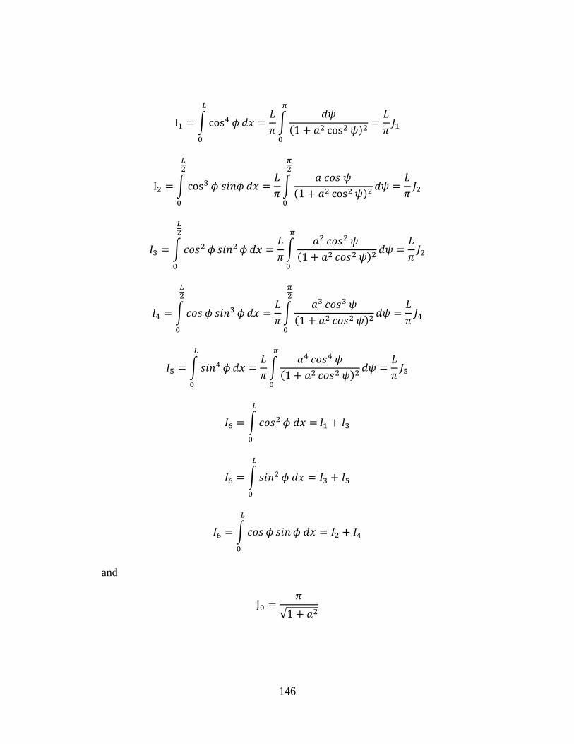
146

I1 = ∫cos4 𝜙𝑑𝑥 =

𝐿

𝜋∫

𝑑𝜓

(1 + 𝑎2 cos2𝜓)2=𝐿

𝜋𝐽1

𝜋

0

𝐿

0

I2 = ∫cos3 𝜙 𝑠𝑖𝑛𝜙 𝑑𝑥 =

𝐿

𝜋∫

𝑎 𝑐𝑜𝑠 𝜓

(1 + 𝑎2 cos2𝜓)2𝑑𝜓 =

𝐿

𝜋𝐽2

𝜋2

0

𝐿2

0

𝐼3 = ∫𝑐𝑜𝑠2 𝜙 𝑠𝑖𝑛2𝜙 𝑑𝑥 =

𝐿

𝜋∫

𝑎2 𝑐𝑜𝑠2𝜓

(1 + 𝑎2 𝑐𝑜𝑠2𝜓)2𝑑𝜓 =

𝐿

𝜋𝐽2

𝜋

0

𝐿2

0

𝐼4 = ∫𝑐𝑜𝑠 𝜙 𝑠𝑖𝑛3 𝜙𝑑𝑥 =

𝐿

𝜋∫


(1 + 𝑎2 𝑐𝑜𝑠2𝜓)2𝑑𝜓 =

𝐿

𝜋𝐽4

𝜋2

0

𝐿2

0

𝐼5 = ∫𝑠𝑖𝑛4 𝜙𝑑𝑥 =𝐿

𝜋∫


(1 + 𝑎2 𝑐𝑜𝑠2𝜓)2𝑑𝜓 =

𝐿

𝜋𝐽5

𝜋

0

𝐿

0

𝐼6 = ∫𝑐𝑜𝑠2 𝜙 𝑑𝑥 =

𝐿

0

𝐼1 + 𝐼3

𝐼6 = ∫𝑠𝑖𝑛2 𝜙 𝑑𝑥 = 𝐼3 + 𝐼5

𝐿

0

𝐼6 = ∫𝑐𝑜𝑠 𝜙 𝑠𝑖𝑛 𝜙 𝑑𝑥 = 𝐼2 + 𝐼4

𝐿

0

and

J0 =𝜋

√1 + 𝑎2

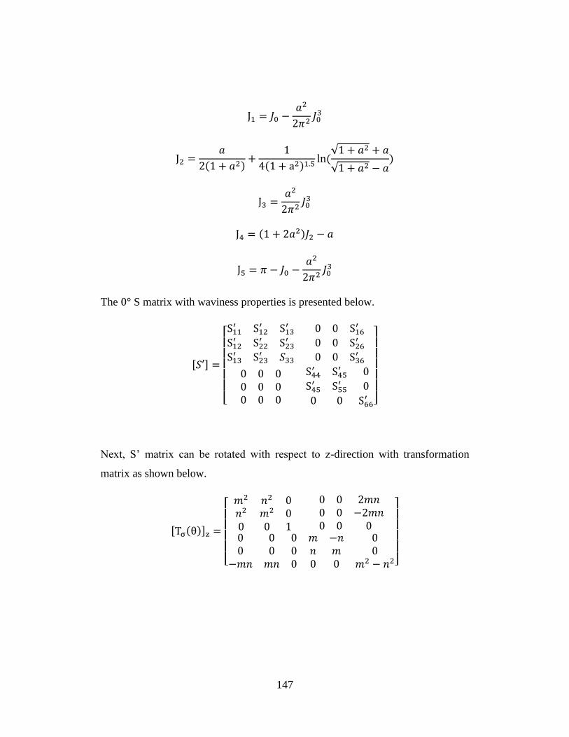
147

J1 = 𝐽0 −𝑎2

2𝜋2𝐽03

J2 =𝑎

2(1 + 𝑎2)+

1

4(1 + a2)1.5ln (√1 + 𝑎2 + 𝑎

√1 + 𝑎2 − 𝑎)

J3 =𝑎2

2𝜋2𝐽03

J4 = (1 + 2𝑎2)𝐽2 − 𝑎

J5 = 𝜋 − 𝐽0 −𝑎2

2𝜋2𝐽03

The 0° S matrix with waviness properties is presented below.

[𝑆′] =

[ S11′ S12

′ S13′

S12′ S22

′ S23′

S13′ S23

′ 𝑆33

0 0 S16′

0 0 S26′

0 0 S36′

0 0 00 0 00 0 0

S44′ S45

′ 0

S45′ S55

′ 0

0 0 S66′ ]

Next, S’ matrix can be rotated with respect to z-direction with transformation

matrix as shown below.

[Tσ(θ)]z =

[ 𝑚2 𝑛2 0𝑛2 𝑚2 00 0 1

0 0 2𝑚𝑛0 0 −2𝑚𝑛0 0 0

0 0 00 0 0

−𝑚𝑛 𝑚𝑛 0

𝑚 −𝑛 0𝑛 𝑚 00 0 𝑚2 − 𝑛2]

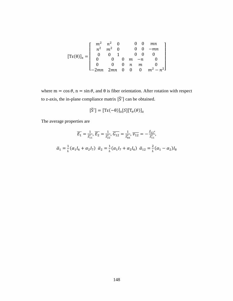
148

[Tε(θ)]z =

[

𝑚2 𝑛2 0𝑛2 𝑚2 00 0 1

0 0 𝑚𝑛0 0 −𝑚𝑛0 0 0

0 0 00 0 0

−2𝑚𝑛 2𝑚𝑛 0

𝑚 −𝑛 0𝑛 𝑚 00 0 𝑚2 − 𝑛2]

where m = cos 𝜃, n = sin 𝜃, and θ is fiber orientation. After rotation with respect

to z-axis, the in-plane compliance matrix [S′] can be obtained.

[S′] = [Tε(−θ)]z[𝑆][Tσ(𝜃)]z

The average properties are

𝐸1 =1

��11′ , 𝐸2 =

1

��22′ , 𝐺12 =

1

��66′ , 𝑣12 = −

��12′

��11′ ,

��1 =1

𝐿(𝛼1𝐼6 + 𝛼2𝐼7) ��2 =

1

𝐿(𝛼1𝐼7 + 𝛼2𝐼6) ��12 =

2

𝐿(𝛼1 − 𝛼2)𝐼8

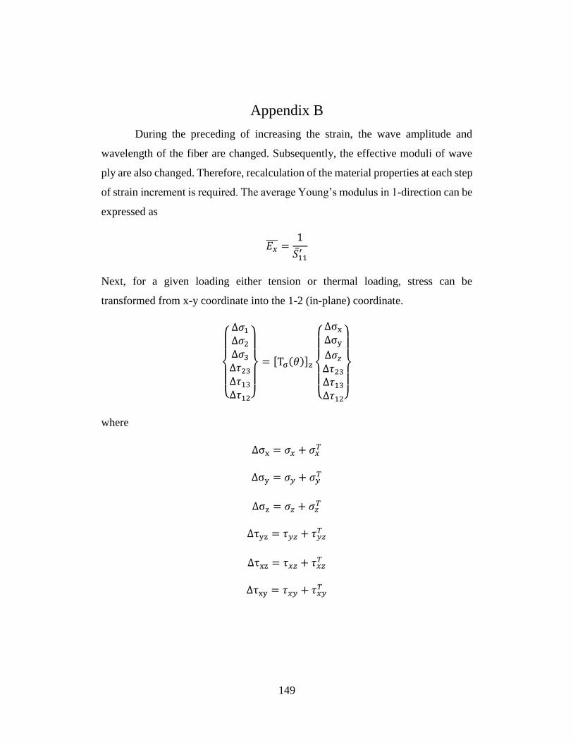
149

Appendix B

During the preceding of increasing the strain, the wave amplitude and

wavelength of the fiber are changed. Subsequently, the effective moduli of wave

ply are also changed. Therefore, recalculation of the material properties at each step

of strain increment is required. The average Young’s modulus in 1-direction can be

expressed as

𝐸𝑥 =1

𝑆11′

Next, for a given loading either tension or thermal loading, stress can be

transformed from x-y coordinate into the 1-2 (in-plane) coordinate.

{

Δ𝜎1Δ𝜎2Δ𝜎3Δ𝜏23Δ𝜏13Δ𝜏12}

= [Tσ(𝜃)]z

{

ΔσxΔσyΔ𝜎𝑧Δ𝜏23Δ𝜏13Δ𝜏12}

where

Δσx = 𝜎𝑥 + 𝜎𝑥𝑇

Δσy = 𝜎𝑦 + 𝜎𝑦𝑇

Δσz = 𝜎𝑧 + 𝜎𝑧𝑇

Δτyz = 𝜏𝑦𝑧 + 𝜏𝑦𝑧𝑇

Δτxz = 𝜏𝑥𝑧 + 𝜏𝑥𝑧𝑇

Δτxy = 𝜏𝑥𝑦 + 𝜏𝑥𝑦𝑇

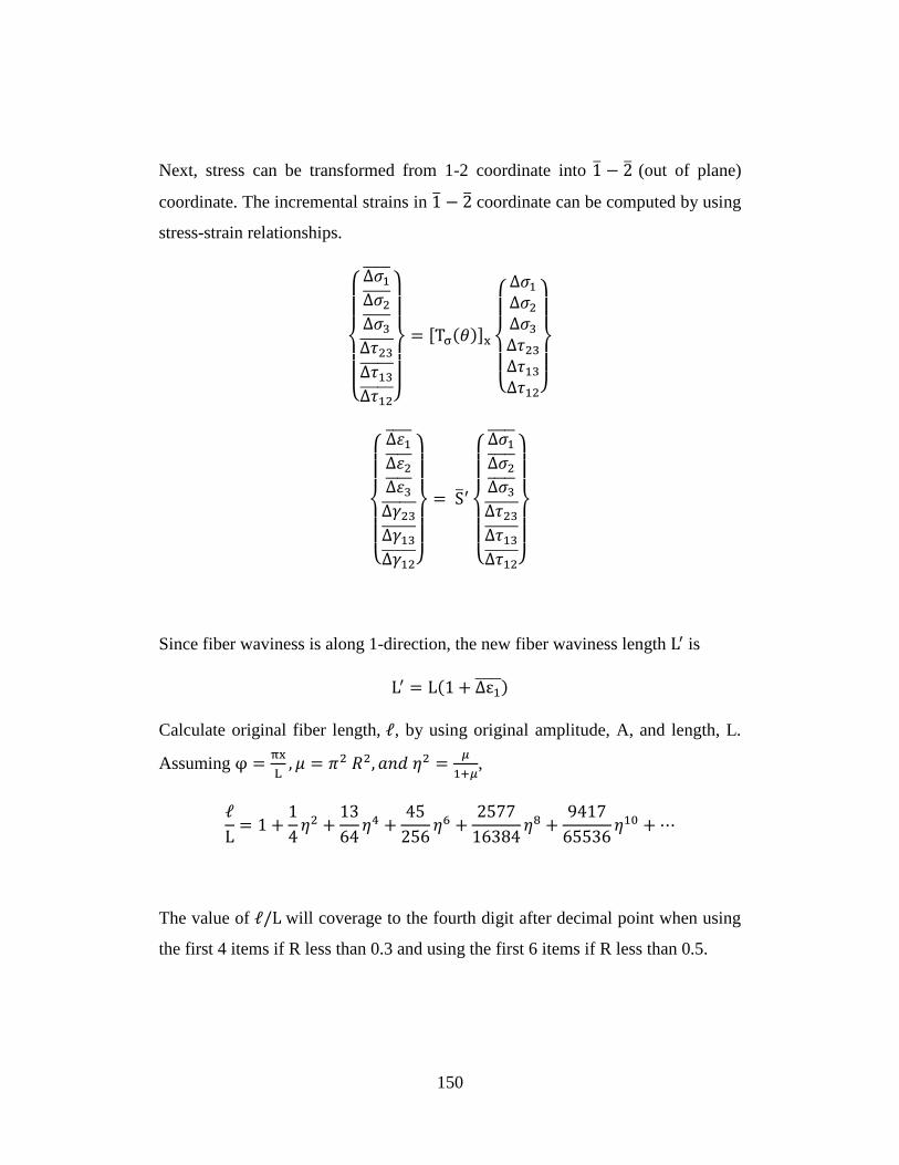
150

Next, stress can be transformed from 1-2 coordinate into 1 − 2 (out of plane)

coordinate. The incremental strains in 1 − 2 coordinate can be computed by using

stress-strain relationships.

{

Δ𝜎1

Δ𝜎2

Δ𝜎3

Δ𝜏23

Δ𝜏13

Δ𝜏12 }

= [Tσ(𝜃)]x

{


{

Δ𝜀1

Δ𝜀2

Δ𝜀3

Δ𝛾23

Δ𝛾13

Δ𝛾12 }

= S′

{

Δ𝜎1

Δ𝜎2

Δ𝜎3

Δ𝜏23

Δ𝜏13

Δ𝜏12 }

Since fiber waviness is along 1-direction, the new fiber waviness length L′ is

L′ = L(1 + Δε1 )

Calculate original fiber length, ℓ, by using original amplitude, A, and length, L.

Assuming φ =πx

L, 𝜇 = 𝜋2 𝑅2, 𝑎𝑛𝑑 𝜂2 =

𝜇

1+𝜇,

ℓ

L= 1 +

1

4𝜂2 +

13

64𝜂4 +

45

256𝜂6 +

2577

16384𝜂8 +

9417

65536𝜂10 +⋯

The value of ℓ/L will coverage to the fourth digit after decimal point when using

the first 4 items if R less than 0.3 and using the first 6 items if R less than 0.5.

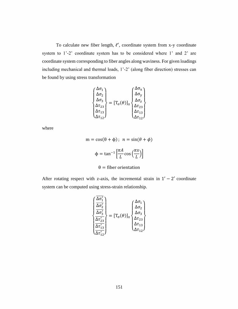
151

To calculate new fiber length, ℓ′, coordinate system from x-y coordinate

system to 1’-2’ coordinate system has to be considered where 1’ and 2’ are

coordinate system corresponding to fiber angles along waviness. For given loadings

including mechanical and thermal loads, 1’-2’ (along fiber direction) stresses can

be found by using stress transformation

{


= [Tσ(𝜃)]z

{

ΔσxΔσyΔ𝜎𝑧Δ𝜏23Δ𝜏13Δ𝜏12}

where

m = cos(θ + ϕ) ; 𝑛 = sin(𝜃 + 𝜙)

ϕ = tan−1 [𝜋𝐴

𝐿cos (

𝜋𝑥

𝐿)]

θ = fiber orientation

After rotating respect with z-axis, the incremental strain in 1′ − 2′ coordinate

system can be computed using stress-strain relationship.

{

Δ𝜎1

′

Δ𝜎2′

Δ𝜎3′

Δ𝜏23′

Δ𝜏13′

Δ𝜏12′ }

= [Tσ(𝜃)]z

{


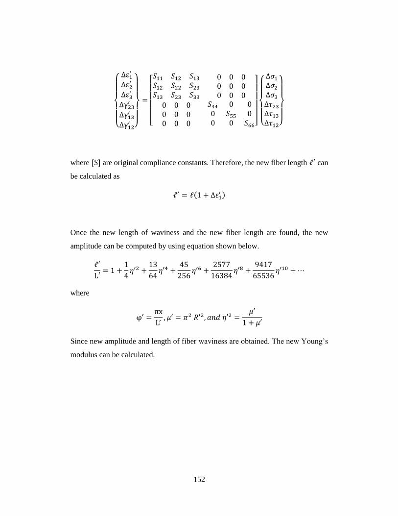
152

{

Δε1

′

Δε2′

Δε3′

Δγ23′

Δγ13′

Δγ12′ }

=

[ 𝑆11 𝑆12 𝑆13𝑆12 𝑆22 𝑆23𝑆13 𝑆23 𝑆33

0 0 00 0 00 0 0

0 0 00 0 00 0 0

𝑆44 0 00 𝑆55 00 0 𝑆66]

{


where [S] are original compliance constants. Therefore, the new fiber length ℓ′ can

be calculated as

ℓ′ = ℓ(1 + Δε1′ )

Once the new length of waviness and the new fiber length are found, the new

amplitude can be computed by using equation shown below.

ℓ′

L′= 1 +

1

4𝜂′2 +

13

64𝜂′4 +

45

256𝜂′6 +

2577

16384𝜂′8 +

9417

65536𝜂′10 +⋯

where

φ′ =πx

L′, 𝜇′ = 𝜋2 𝑅′2, 𝑎𝑛𝑑 𝜂′2 =

𝜇′

1 + 𝜇′

Since new amplitude and length of fiber waviness are obtained. The new Young’s

modulus can be calculated.

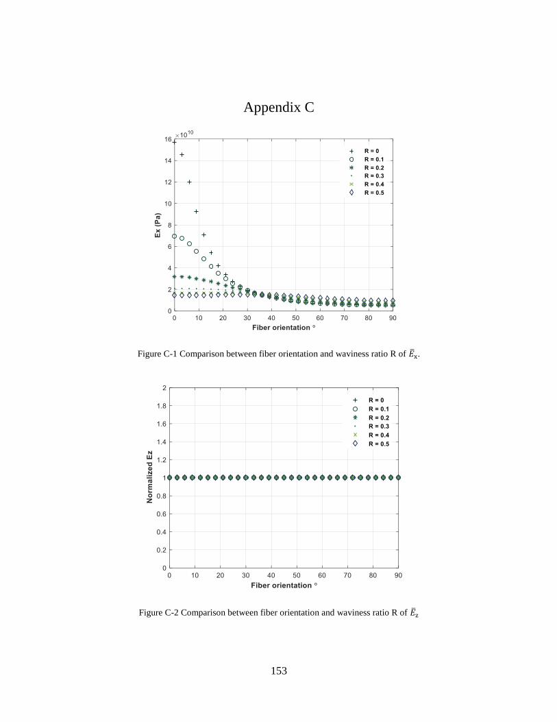
153

Appendix C

Figure C-1 Comparison between fiber orientation and waviness ratio R of ��x.

Figure C-2 Comparison between fiber orientation and waviness ratio R of ��z

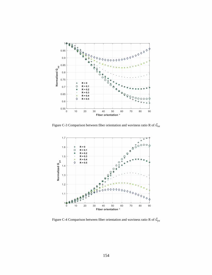
154

Figure C-3 Comparison between fiber orientation and waviness ratio R of ��xz

Figure C-4 Comparison between fiber orientation and waviness ratio R of ��yz

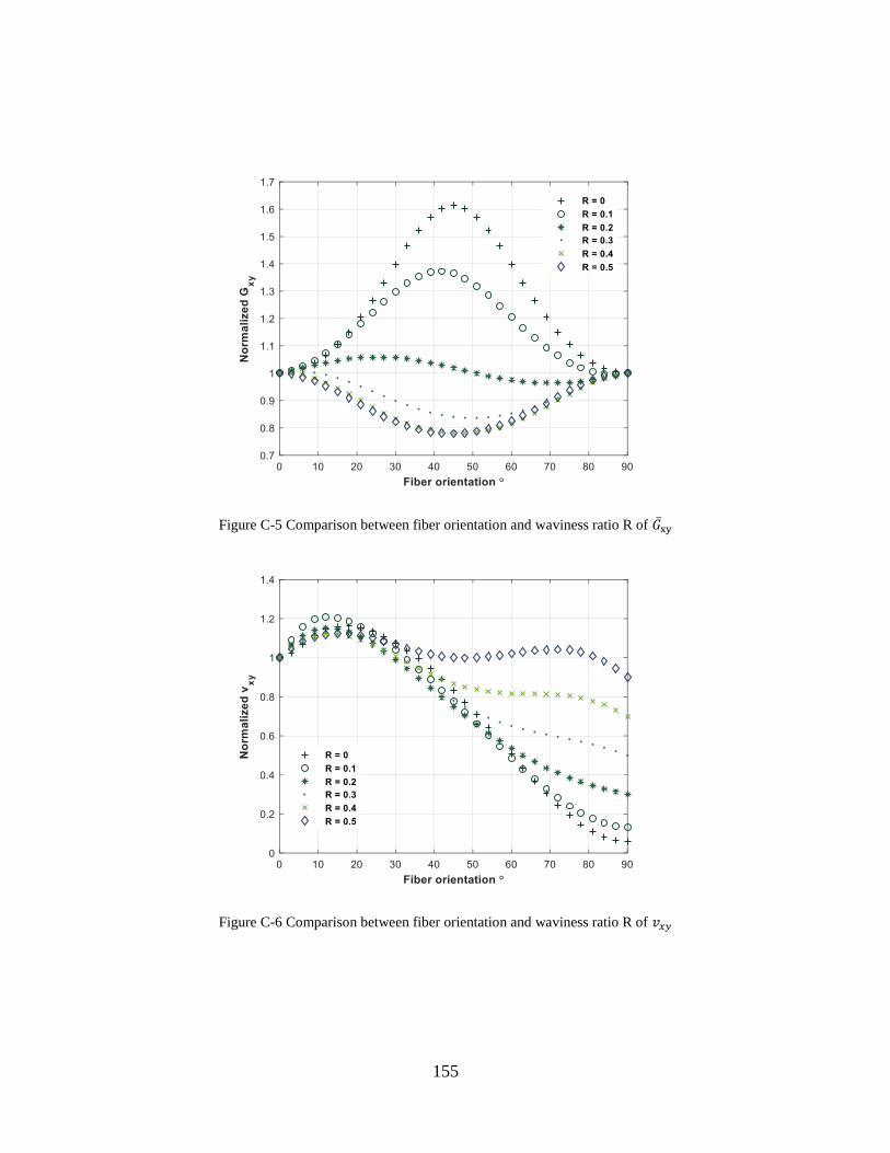
155

Figure C-5 Comparison between fiber orientation and waviness ratio R of ��xy

Figure C-6 Comparison between fiber orientation and waviness ratio R of 𝑣𝑥𝑦

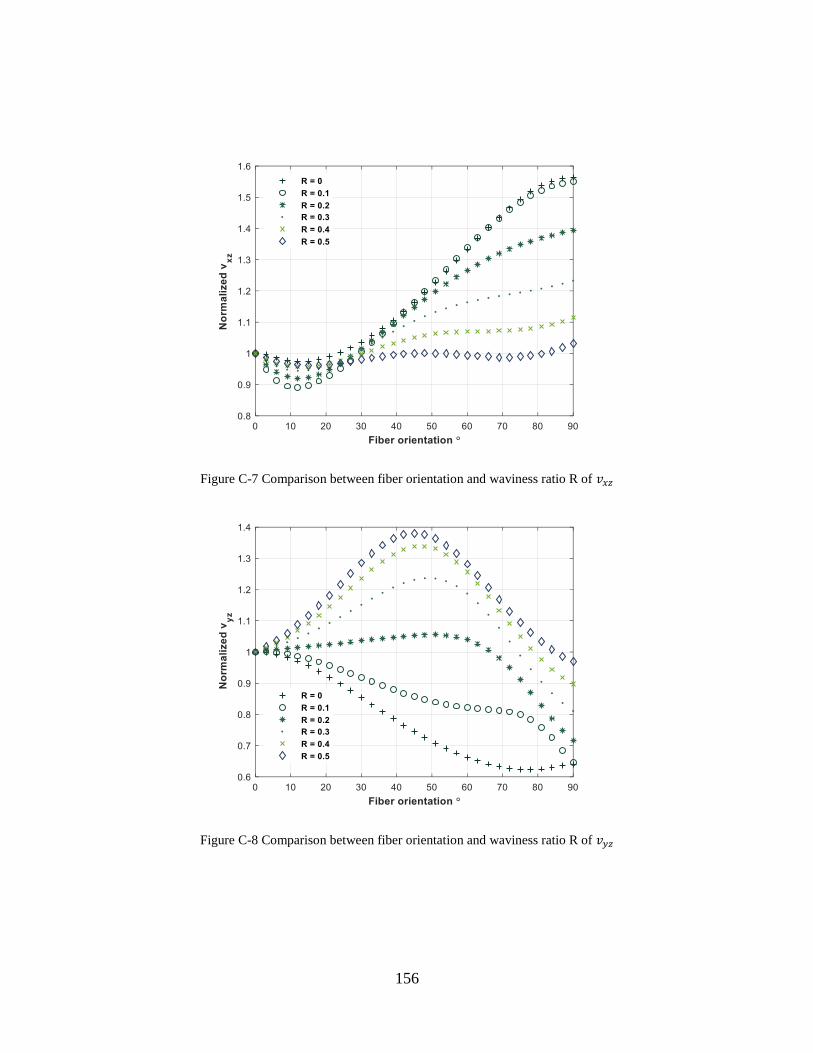
156

Figure C-7 Comparison between fiber orientation and waviness ratio R of 𝑣𝑥𝑧

Figure C-8 Comparison between fiber orientation and waviness ratio R of 𝑣𝑦𝑧

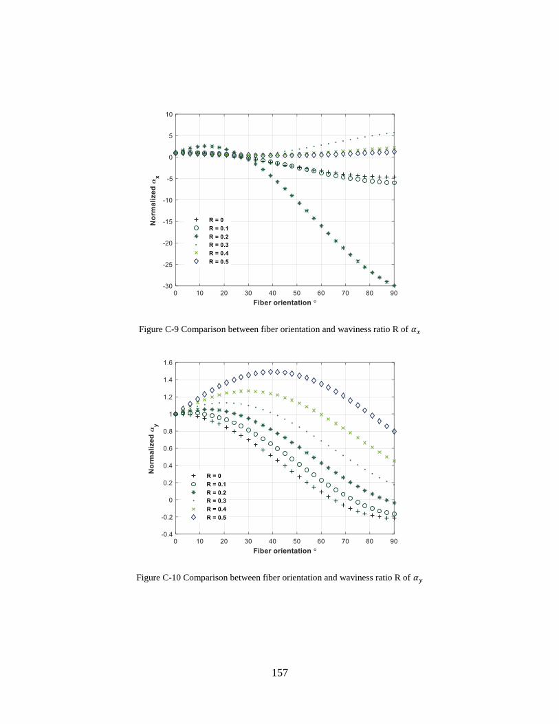
157

Figure C-9 Comparison between fiber orientation and waviness ratio R of 𝛼𝑥

Figure C-10 Comparison between fiber orientation and waviness ratio R of 𝛼𝑦

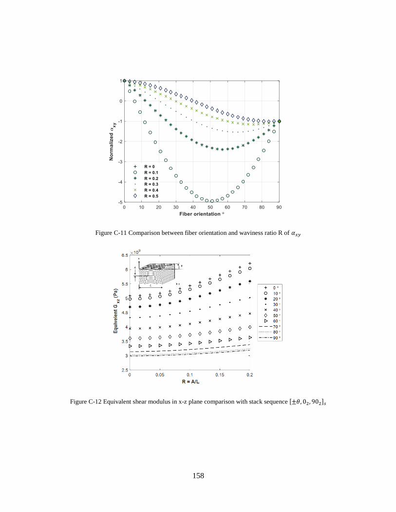
158

Figure C-11 Comparison between fiber orientation and waviness ratio R of 𝛼𝑥𝑦

Figure C-12 Equivalent shear modulus in x-z plane comparison with stack sequence [±𝜃, 02, 902]𝑠

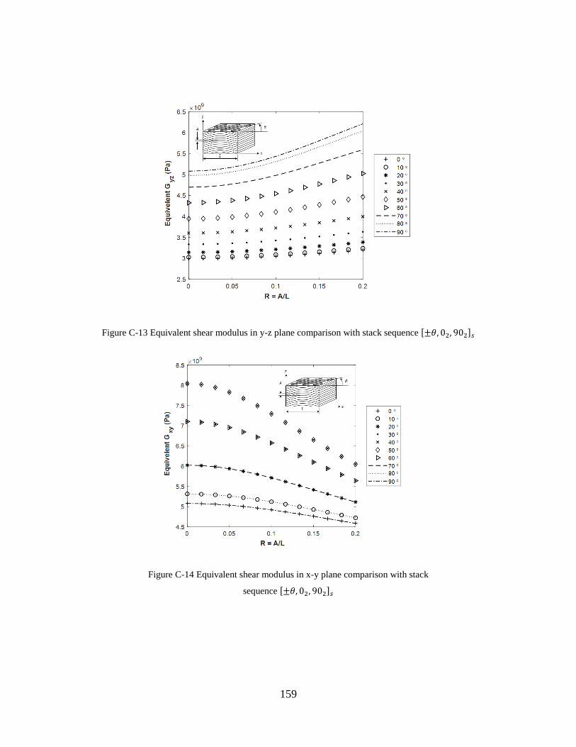
159

Figure C-13 Equivalent shear modulus in y-z plane comparison with stack sequence [±𝜃, 02, 902]𝑠

Figure C-14 Equivalent shear modulus in x-y plane comparison with stack


160

REFERENCE

1. Love, A. E. H. (1888). The small free vibrations and deformation of a thin elastic shell.

Philosophical Transactions of the Royal Society of London. A, 179, 491-546.

2. Timoshenko, S. P., 1921, On the correction factor for shear of the differential equation for

transverse vibrations of bars of uniform cross-section, Philosophical Magazine, p. 744.

3. TIMOSHENKSO.., A N D J . N. GOODIER.1 951. Theory of elasticity. 2nd ed. McGraw-

Hill, N.Y. Pp.

4. ODEN. T. J. 1967. Mechanics of elastic structures. McGraw-Hill, N.Y.

5. Lekhnitskii, S. G. (1968). Anisotropic plates (No. FTD-HT-23-608-67). Foreign Technology

Div Wright-Patterson Afb Oh.

6. Cheung, C. K., & Sorensen, H. C. (1982). Effect of axial loads on radial stress in curved

beams. Wood and Fiber Science, 15(3), 263-275.

7. Tolf, G. (1983). Stresses in a curved laminated beam. Fibre Science and Technology, 19(4),

243-267.

8. Ko, W. L. (1988). Delamination stresses in semicircular laminated composite bars.

9. Shenoi, R. A., & Wang, W. (2001). Through-thickness stresses in curved composite

laminates and sandwich beams. Composites Science and Technology, 61(11), 1501-1512.

10. Ko, W. L., & Jackson, R. H. (1989). Multilayer theory for delamination analysis of a

composite curved bar subjected to end forces and end moments. In Composite structures 5

(pp. 173-198). Springer, Dordrecht.

11. Wang, W., & Shenoi, R. A. (2004). Analytical solutions to predict flexural behavior of

curved sandwich beams. Journal of Sandwich Structures & Materials, 6(3), 199-216.

12. Ko, W. L., & Jackson, R. H. (1989). Multilayer theory for delamination analysis of a

composite curved bar subjected to end forces and end moments. In Composite structures 5

(pp. 173-198). Springer, Dordrecht.

13. Nguyen, T. (2010). Effects of Curvature on the Stresses of a Curved Laminated Beams

subjected to Bending.

14. Sushanta G. & Kashinath S. (2017). A review on stress and deformation analysis of cirved

beams under large deflection. International Journal of Engineering and Technologies.

15. Qatu, M. S. (1993). Theories and analyses of thin and moderately thick laminated composite

curved beams. International Journal of Solids and Structures, 30(20), 2743-2756.

16. Erkmen, R. E., & Bradford, M. A. (2009). Nonlinear elastic analysis of composite beams

curved in-plan. Engineering Structures, 31(7), 1613-1624.

17. Aggarwal, M. (2016). Analysis of curved composite beam. West Virginia University.

18. Tan, E. L., & Uy, B. (2009). Experimental study on curved composite beams subjected to

combined flexure and torsion. Journal of Constructional Steel Research, 65(8-9), 1855-1863.

19. Yu, W., Hodges, D. H., Volovoi, V., & Cesnik, C. E. (2002). On Timoshenko-like modeling

of initially curved and twisted composite beams. International Journal of Solids and

Structures, 39(19), 5101-5121.

20. Zhang, Y., Hou, Z., Li, Y., & Wang, Y. (2015). Torsional behaviour of curved composite

beams in construction stage and diaphragm effects. Journal of Constructional Steel Research,

108, 1-10.

21. Lee, J., & Soutis, C. (2007) A study on the compressive strength of thick carbon fibre-epoxy

laminates. Composite science and technology, 67(10), 2015-2026.

161

22. Kantharaju, H. (2012). Analysis of fiber waviness in laminated composite subjected to

compressive loads (Doctoral dissertation, Wichita State University).

23. Kugler, D., & Moon, T. J. (2002). Identification of the most significant processing

parameters on the development of fiber waviness in thin laminates. Journal of Composite

Materials, 36(12), 1451-1479.

24. Yousaf, Z. (2014). Investigation of deformation behaviour of dry textiles under forming

forces by computed tomography(Doctoral dissertation, University of Manchester).

25. Masters, J. E., Naik, R., & Minguet, P. J. (1995). Effects of preform architecture on modulus

and strength of 2-D triaxially braided textile composites

26. Minguet, P. (1994, July). A comparison of graphite/epoxy tape laminates and 2-D braided

composites mechanical properties. In 36th Structures, Structural Dynamics and Materials

Conference (p. 1158).

27. Jackson, W. C., & Portanova, M. A. (1995). Out-of-plane properties.

28. Whitcomb, J., & Srirengan, K. (1996). Effect of various approximations on predicted

progressive failure in plain weave composites. Composite structures, 34(1), 13-20.

29. Mahadik, Y., & Hallett, S. R. (2011). Effect of fabric compaction and yarn waviness on 3D

woven composite compressive properties. Composites Part A: Applied Science and

Manufacturing, 42(11), 1592-1600.

30. Yushanov, S. P., & Bogdanovich, A. E. (2000). Fiber waviness in textile composites and its

stochastic modeling. Mechanics of Composite materials, 36(4), 297-318.

31. Bolotin, V. V. (1966). Theory of a reinforced layered medium with random initial

irregularities. Polymer mechanics, 2(1), 7-11.

32. Tarnopol'skii, Y. M., Portnov, G. G., & Zhigun, I. G. (1967). Effect of fiber curvature on the

modulus of elasticity for unidirectional glass-reinforced plastics in tension. Polymer

Mechanics, 3(2), 161-166.

33. Bažant, Z. P. (1968). Effect of Curvature of the Reinforcing Fibers on the Moduli of

Elasticity and Strength of Composites. Polymer Mechanics, 4(2), 251-258.

34. Lin, K. Y., & Zhang, X. J. (1992). Effect of fiber waviness on the compressive strength of

laminated composites. In The Second International Symposium on Composite Materials and

Structures(pp. 120-125).

35. Wisnom, M. R. (1990). The effect of fibre misalignment on the compressive strength of

unidirectional carbon fibre/epoxy. Composites, 21(5), 403-407.

36. Camponeschi, E. T. (1991). Lamina waviness levels in thick composites and its effect on

their compression strength. Composites.

37. Lo, K. H., & Chim, E. M. (1992). Compressive strength of unidirectional

composites. Journal of Reinforced Plastics and Composites, 11(8), 838-896.

38. O'Hare Adams, D., & Hyer, M. W. (1993). Effects of layer waviness on the compression

strength of thermoplastic composite laminates. Journal of Reinforced Plastics and

Composites, 12(4), 414-429.

39. Rai, H. G., Rogers, C. W., & Crane, D. A. (1992). Mechanics of curved fiber

composites. Journal of reinforced plastics and composites, 11(5), 552-566.

40. Bogetti, T. A., Gillespie Jr, J. W., & Lamontia, M. A. (1992). Influence of ply waviness on

the stiffness and strength reduction on composite laminates. Journal of Thermoplastic

Composite Materials, 5(4), 344-369.

162

41. Bogetti, T. A., Gillespie Jr, J. W., & Lamontia, M. A. (1994). The influence of ply waviness

with nonlinear shear on the stiffness and strength reduction of composite laminates. Journal

of Thermoplastic Composite Materials, 7(2), 76-90.

42. Chan, W. S., & Wang, J. S. (1994). Influence of fiber waviness on the structural response of

composite laminates. Journal of Thermoplastic Composite Materials, 7(3), 243-260.

43. Chan, W. S., & Chou, C. J. (1995). Effects of delamination and ply fiber waviness on

effective axial and bending stiffnesses in composite laminates. Composite structures, 30(3),

299-306.

44. Garnich, M. R., & Karami, G. (2005). Localized fiber waviness and implications for failure

in unidirectional composites. Journal of composite materials, 39(14), 1225-1245.

45. Hsiao, H. M., & Daniel, I. M. (1996). Effect of fiber waviness on stiffness and strength

reduction of unidirectional composites under compressive loading. Composites science and

technology, 56(5), 581-593.

46. Hsiao, H. M., & Daniel, I. M. (1996). Nonlinear elastic behavior of unidirectional

composites with fiber waviness under compressive loading. Journal of Engineering Materials

and Technology, 118(4), 561-570.

47. Hsiao, H. M., & Daniel, I. M. (1996). Elastic properties of composites with fiber

waviness. Composites Part A: Applied Science and Manufacturing, 27(10), 931-941.

48. Seon, G. (2009). Finite element-based failure models for carbon/epoxy tape

composites (Doctoral dissertation, Georgia Institute of Technology).

49. Nikishkov, Y., Makeev, A., & Seon, G. (2013). Progressive fatigue damage simulation

method for composites. International Journal of Fatigue, 48, 266-279.

50. Evans, F. J. (1969). U.S. Patent No. 3,485,706. Washington, DC: U.S. Patent and Trademark

Office.

51. Sainsbury-Carter JB. Braided composites: a material form providing low cost fabrication

techniques. In: National SAMPE symposium and exhibition (proceedings), vol. 30; 1985. p.

1486–97.

52. Masters, J. E., Naik, R., & Minguet, P. J. (1995). Effects of preform architecture on modulus

and strength of 2-D triaxially braided textile composites

53. Minguet, P. (1994, July). A comparison of graphite/epoxy tape laminates and 2-D braided

composites mechanical properties. In 36th Structures, Structural Dynamics and Materials

Conference (p. 1158).

54. Jackson, W. C., & Portanova, M. A. (1995). Out-of-plane properties.

55. Whitcomb, J., & Srirengan, K. (1996). Effect of various approximations on predicted

progressive failure in plain weave composites. Composite structures, 34(1), 13-20.

56. Yushanov, S. P., & Bogdanovich, A. E. (2000). Fiber waviness in textile composites and its

stochastic modeling. Mechanics of Composite materials, 36(4), 297-318.

57. Tarnopol'skii, Y. M. (1991). Spatially reinforced composites. CRC Press.

58. Bogdanovich, A., Pastore, C. M., & Pastore, C. (1996). Mechanics of textile and laminated

composites: with applications to structural analysis. Springer Science & Business Media.

59. Arumugam, V., Kumar, C. S., Santulli, C., Sarasini, F., & Stanley, A. J. (2013).

Identification of failure modes in composites from clustered acoustic emission data using

pattern recognition and wavelet transformation. Arabian Journal for Science and

Engineering, 38(5), 1087-1102.

163

60. O'Brien, T. K. (1984). Interlaminar Fracture of Composites (No. NASA-TM-85768).

NATIONAL AERONAUTICS AND SPACE ADMINISTRATION HAMPTON VA

LANGLEY RESEARCH CEN TER.

61. King, Y. (1991). Delamination analysis of a laminated composite tapered beam. Texas

Univ., Arlington, TX (United States).

62. Wilkins, D. J., Eisenmann, J. R., Camin, R. A., Margolis, W. S., & Benson, R. A. (1982).

Characterizing delamination growth in graphite-epoxy. In Damage in Composite Materials:

Basic Mechanisms, Accumulation, Tolerance, and Characterization. ASTM International.

63. Lagace, P., Brewer, J. O. H. N., & Kassapoglou, C. (1987). The effect of thickness on

interlaminar stresses and delamination in straight-edged laminates. Journal of Composites,

Technology and Research, 9(3), 81-87.

64. O'Brien, T. K. (1984). Mixed-mode strain-energy-release rate effects on edge delamination

of composites. In Effects of defects in composite materials. ASTM International.

65. Wang, A. S. D., & Crossman, F. W. (1977). Some new results on edge effect in symmetric

composite laminates. Journal of Composite Materials, 11(1), 92-106.

66. Pipes, R. B., & Pagano, N. J. (1994). Interlaminar stresses in composite laminates under

uniform axial extension. In Mechanics of composite materials (pp. 234-245). Springer,

Dordrecht.

67. AC09036782, A. (Ed.). (2007). Standard test method for mode I interlaminar fracture

toughness of unidirectional fiber-reinforced polymer matrix composites. ASTM Internat..

68. WK22949, A. S. T. M. (2009). New Test Method for Determination of the Mode II

Interlaminar Fracture Toughness of Unidirectional Fiber-reinforced Polymer Matrix

Composites using the End-notched flexure (ENF) Test. American Society for Testing and

Materials, West Conshohocken.

69. Jain, L. K., & Mai, Y. W. (1995). Determination of mode II delamination toughness of

stitched laminated composites. Composites Science and Technology, 55(3), 241-253.

70. Massabo, R., & Cox, B. N. (1999). Concepts for bridged mode II delamination

cracks. Journal of the Mechanics and Physics of Solids, 47(6), 1265-1300.

71. Massabò, R., Mumm, D. R., & Cox, B. (1998). Characterizing mode II delamination cracks

in stitched composites. International Journal of Fracture, 92(1), 1-38.

72. Song, S. J., & Waas, A. M. (1995). Energy-based mechanical model for mixed mode failure

of laminated composites. AIAA journal, 33(4), 739-745.

73. Lu, T. J., Xia, Z. C., & Hutchinson, J. W. (1994). Delamination of beams under transverse

shear and bending. Materials Science and Engineering: A, 188(1-2), 103-112.

74. Martin, R. H., & Jackson, W. C. (1993). Damage prediction in cross-plied curved composite

laminates. In Composite Materials: Fatigue and Fracture, Fourth Volume. ASTM

International.

75. Massabò, R., & Cox, B. N. (1999). Bridged Delamination Cracks in Curved Beams and

Mixed-Mode Bending Specimens. Proc. ICCM12, Paris.

76. Bruno, D., Carpino, R., Greco, F., & Lonetti, P. (2006). Energy release rate and mode

partition for interlaminar crack in circular laminated beams. International journal of solids

and structures, 43(5), 1201-1223.

77. Shams, S. (2016). Experimental, Analytical and Numerical Characterization of Effects of

Fiber Waviness Defects in Laminated Composites.

78. Chun, H. J. (2002). Evaluation of fiber waviness in thick composites by ultrasonic test. In

Recent Advances in Experimental Mechanics (pp. 433-442). Springer, Dordrecht.

164

79. Chun, H. J., Shin, J. Y., & Daniel, I. M. (2000). Nonlinear behavior of thick composites with

uniform fiber waviness. AIAA journal, 38(10), 1949-1955.

80. Ye, T., Jin, G., Ye, X., & Wang, X. (2015). A series solution for the vibrations of composite

laminated deep curved beams with general boundaries. Composite Structures, 127, 450-465.

81. González-Cantero, J. M., Graciani, E., Blázquez, A., & París, F. (2014, June). Analytic

evaluation of radial stresses in unfolding failure of composite materials. Comparison with

numerical solutions. In Proceedings of the 16th European Conference on Composite

Materials ECCM16 (pp. 22-26).

82. González Cantero, J. M. (2017). Study of the unfolding failure of curved composite

laminates.

83. Abaqus/Standard, V6.14-2, is a trademark of ABAQUS, Inc.

84. Makeev, A., Seon, G., Nikishkov, Y., Nguyen, D., Mathews, P., & Robeson, M. (2015).

Analysis Methods for Improving Confidence in Material Qualification for Laminated

Composites. Journal of the American Helicopter Society, 64(1), 1-13.

85. Rybicki, E. F., & Kanninen, M. F. (1977). A finite element calculation of stress intensity

factors by a modified crack closure integral. Engineering fracture mechanics, 9(4), 931-938.

86. Benzeggagh, M.L. and M. Kenane. 1996. "Measurement of Mixed-Mode Delamination

Fracture Toughness of Unidirectional Glass/Epoxy Composites with Mixed-Mode Bending

Apparatus." Comp Sci & Tech, 56(4):439-449.

87. Allegri, G., Wisnom, M. R., & Hallett, S. R. (2013). A new semi-empirical law for variable

stress-ratio and mixed-mode fatigue delamination growth. Composites Part A: Applied

Science and Manufacturing, 48, 192-200.

88. Vasiliev, V. V. and R. M., Jones. Chapter 4 in Mechanics of Composite Structures, Taylor &

Francis, Washington, DC, 1993.

89. Barbero, E.J. Chapter 8 in Introduction to Composite Materials Design, Taylor & Francis,

Washington, DC., 1998.

90. Kollar, L. P. and G. S. Springer. Chapter 8 in Mechanics of Composite Structures,

Cambridge University Press, UK, 2003.

91. Liberscu, L. and O. Song. Thin-Walled Composite Beams-Theory and Application, Springer,

the Netherlands, 2006.

92. Hodges, D. Nonlinear Analysis of Composite Structures, Cambridge University Press, UK,

2008.

93. Wu, X.-X. and C. T. Sun. “Simplified Theory for Composite Thin-Walled Beams’ AIAA

Journal, 1992. Vol. 30, No. 12, pp 2945-2951.

94. Yu, W., D. H. Hodges, V. V. Volovoi, and D. F. Eduardo. "A Generalized Vlasov Theory of

Composite Beams," Thin-Walled Structures, vol. 43, no. 9, pp.1493-1511. 2005.

95. Yu, W.. J. C. Ho, and D. H. Hodges. "Variational Asymptotic Beam Sectional Analysis --

An Updated Version," International Journal of Engineering Science, vol. 59, pp. 40-64.

2012.

96. Drummond, J. A., and W. S. Chan. “Fabrication, Analysis, and Experimentation of a

Practically Constructed Laminated Composite I-Beam under Pure Bending”, Journal of

Thermoplastic Composite Materials, May Issue, pp. 177-187. 1999

97. Jung, S. N., and J. Y. Lee.“Closed-form Analysis of Thin-walled Composite I-beams

Considering Non-classical Effects”, Composite Structures Vol.60, 2003, pp. 9–17. 2003.

98. Rios, G. and W.S. Chan.“A Unified Analysis of Stiffener Reinforced Composite Beams”,

25th Annual Technical Conference of American Society for Composites. 2010.

165

99. Parambil, J.C., W.S. Chan., K.L. Lawrence, V. Sanghai.“Stress Analysis of Composite I-

Beam by a Non –Conventional Method”, Proceedings of the American Society for

Composites 26th Technical Conference, paper No. 1027. 2011.

100. Sanghai, V. and W.S. Chan. “Torsional Analysis of a Composite I-Beam”, Proceedings of

the American Society for Composites 28th Technical Conference. 2013.

101. Syed, K. A., and W. S. Chan. September 2006. “Analysis of Hat-Sectioned Reinforced

Composite Beams”, Proceedings of the 28th Technical Conference of American Society for

Composites, Paper No. 1055.

102. T.H.G. Megson, Aircraft Structures for engineering students, Third edition, Butterworth

Heinemann publications, 1999.

103. https://www.fxsolver.com/browse/formulas/Torsion+constant+%28Rectangle%29

104. Walter D. Pilkey and K. Kevent. “Notes on the Linear Analysis of Thins-walled Beams”.

University of Virginia, 1996.

105. Robert L. Ketter, George C. Lee and Sherwood P. Prawel, Jr., Structural Analysis and

design, McGraw-Hill Inc, 1979

106. Singh, S.“A Novel Stress Analysis Method For Laminated Composite Stiffener With

Asymmetric Z-Section Under Mechanical And Thermal Loading Conditions”, Master thesis

of Aerospace Engineering program, Department of Mechanical and Aerospace Engineering,

The University of Texas at Arlington. 2016.

107. Lu, W. T., Singh, S., & Chan, W. S. (2019). A novel stress analysis method for composite Z-

stiffeners under mechanical and thermal loads. Journal of Composite Materials,

0021998319846947.

108. Sanghavi, V. M. S. (2013). Torsional Analysis of a Composite I-beam.

109. Kollár, L. P., & Springer, G. S. (2003). Mechanics of composite structures.

110. ANSYS Academic Research, Release 17.2. 2017: Canonsburg, Pennsylvania Cambridge

university press.

111. Lu, W. T. “Effects Of Transverse Shear Deformation On Composite Beams With Various

Laminate Configurations And Boundary Conditions”. Master thesis of Aerospace

Engineering program, Department of Mechanical and Aerospace Engineering, The

University of Texas at Arlington. 2015

112. Gl aucio C. Pereira , P. Leboulluec , W. T. Lu , M. I. Yoshida, Ana P. Alves and Antˆonio.

F. Avila. ”Spring-Back Behavior on L-shaped Composite Structures: a statistical analysis of

angular recovery as a function of time and residual cure”, Composites Part A: Applied

Science and Manufacturing.

https://www.fxsolver.com/browse/formulas/Torsion+constant+%28Rectangle%29

Documents

ANALYSIS OF LAMINATED CURVED BEAM WITH AND WITHOUT …