Analysis of Linear and MonoclinalRiver Wave SolutionsMichael G. Ferrick and Nicholas J. Goodman January 1998

74ItT

Abstract: Linear dynamic wave and diffusion wave to arbitrarily large flow increases. As wave amplitudeanalytical solutions are obtained for a small, abrupt increases the monoclinal rating curve diverges fromflow increase from an initial to a higher steady flow. that for a linear wave, and the maximum Froude num-Equations for the celerities of points along the wave ber and energy gradient along the profile increase andprofiles are developed from the solutions and related move toward the leading edge. A monoclinal-diffu-to the kinematic wave and dynamic wave celerities. sion solution is developed for the diffusion wave equa-The linear solutions are compared systematically in a tions, and dynamic wave-diffusion wave compari-series of case studies to evaluate the differences sons are made over a range of amplitudes with thecaused by inertia. These comparisons use the celeri- same case studies used for linear waves. Generalties of selected profile points, the paths of these points dimensionless monoclinal-diffusion profiles exist foron the x-t plane, and complete profiles at selected each depth ratio across the wave, while correspond-times, indicating general agreement between the solu- ing monoclinal wave profiles exhibit minor, case-tions. Initial diffusion wave inaccuracies persist over specific Froude number dependence. Inertial effects onrelatively short time and distance scales that increase the monoclinal profiles occur near the leading edge,with both the wave diffusion coefficient and Froude increase with the wave amplitude and Froude number,number. The nonlinear monoclinal wave solution par- and are responsible for the differences between theallels that of the linear dynamic wave but is applicable dimensionless profiles.

Cover- Abrupt river wave moving downstream in the Sacandaga River (New York) near itsconfluence with the Hudson River. This surge was formed by a sudden flow increase ofStewarts Bridge Dam several kilometers upstream. (Photo by M Ferrick.)

How to get copies of CRREL technical publications:Department of Defense personnel and contractors may order reports through the Defense Technical Information Center:

DTIC-BR SUITE 09448725 JOHN J KINGMAN RDFT BELVOIR VA 22060-6218Telephone 1 800 225 3842E-mail help@dtic.mil

msorders@dtic.milWWW http://www.dtic.dla.mil/

All others may order reports through the National Technical Information Service:NTIS5285 PORT ROYAL RDSPRINGFIELD VA 22161Telephone 1 703 487 4650

1 703 487 4639 (TDD for the hearing-impaired)E-mail orders@ntis.fedworld.govWWW http://www.fedworld.gov/ntis/ntishome.html

A complete list of all CRREL technical publications is available fromUSACRREL (CECRL-LP)72 LYME RDHANOVER NH 03755-1290Telephone 1 603 646 4338E-mail techpubs@crrel.usace.army.mil

For information on all aspects of the Cold Regions Research and Engineering Laboratory, visit our World Wide Web site:http://www.crrel.usace.army.mil

US Arm Corp sof Eng~inyeers.Cold Regions Research &Engineering Laboratory

Analysis of Linear and MonoclinalRiver Wave SolutionsMichael G. Ferrick and Nicholas J. Goodman January 1998

Prepared far

OFFICE OF THE CHIEF OF ENGINEERS

Approved for public release: distribution is unlimited.

PREFACE

This report was prepared by Michael G. Ferrick, Hydrologist, and Nicholas J.Goodman, Physical Science Aid, Geological Sciences Division, Research and Engi-neering Directorate, U.S. Army Cold Regions Research and Engineering Labora-tory, Hanover, New Hampshire. Funding for this research was provided by DAProject DT 08, Bosnia Support, and by CWIS Project 7VC103, Water Resources of ColdRegions.

The authors thank S. Daly and Dr. K. O'Neill of CRREL, K. Newyear of theUniversity of Washington, Dr. G. Schohl of the Tennessee Valley Authority, andtwo anonymous reviewers for their thoughtful comments that helped to improvethis manuscript. They also thank Dr. Y. Nakano of CRREL for his independentderivation of eq 19.

ii

CONTENTS

P refa ce ................................................................................................................................... iiN om en clatu re ....................................................................................................................... vIn tro d u ction .......................................................................................................................... 1Linear river w ave equations ............................................................................................ 2Solutions for linear dynamic and linear diffusion waves ............................................ 4Nonlinear monoclinal and monoclinal-diffusion waves ........................................... 7Comparison of the linear solutions ................................................................................. 9Analysis of the monoclinal solutions ............................................................................ 14C on clu sion s .......................................................................................................................... 23L iteratu re cited ..................................................................................................................... 24A b stra ct ................................................................................................................................. 2 7

ILLUSTRATIONS

Figure1. Initial and upstream boundary conditions of the linear equations, and

dimensionless p profile development with dimensional distance and time. 42. Dimensionless celerities of selected linear diffusion wave and dynamic wave

p rofile poin ts ...................................................................................................... . . 103. Traces on the x-t plane of selected linear diffusion wave and dynamic wave

p rofile p oin ts ...................................................................................................... . . 114. Comparison between origin positions of the moving coordinate system in

the linear diffusion wave and dynamic wave models for all cases ............. 125. Linear diffusion wave and dynamic wave profiles and small-amplitude

monoclinal wave profile m ................................................................................. 136. Dimensionless monoclinal profile celerity and overrun discharge as a func-

tion of depth ratio ................................................................................................. 157. Evaluation of eq 41 as a function of depth ratio for selected dimensionless

depths on the monoclinal profile ....................................................................... 168. Case I monoclinal and monoclinal-diffusion profiles at two distance scales

for depth ratios ranging between 1.1 and 50 ................................................... 169. Case II monoclinal and monoclinal-diffusion profiles at two distance scales

for depth ratios ranging between 1.1 and 50 ................................................... 1710. Case III monoclinal and monoclinal-diffusion profiles at two distance scales

for depth ratios ranging between 1.1 and 5 ..................................................... 1711. Case IV monoclinal and monoclinal-diffusion profiles at two distance scales

for depth ratios ranging between 1.1 and 10 ................................................... 1812. Case V monoclinal and monoclinal-diffusion profiles at two distance scales

for depth ratios ranging between 1.1 and 35 ................................................... 1913. General monoclinal-diffusion profiles at two dimensionless distance scales

for depth ratios ranging between 1.1 and 50 ................................................... 19

iii

Figure14. Monoclinal profiles for all cases at two dimensionless distance scales for

depth ratios ranging between 1.1 and 10 ........................................................ 2015. Dimensionless monoclinal and steady state rating curves for depth ratios

ranging betw een 2 and 50 ................................................................................. 2116. Energy gradient and Froude number parameter E along the monoclinal

wave profile for selected depth ratios ............................................................. 2117. Energy gradient and Froude number parameter E as a function of depth

ratio for selected dimensionless depths along the profile ............................ 2218. Dimensionless depth and corresponding maximum E as functions of depth

ra tio ............................................................................................................................ 2 2

TABLE

Table1. Case studies used to compare solutions ................................................................. 9

iv

NOMENCLATURE

B monoclinal wave overrun unit discharge (m3 /s.m)

e dimensionless celerity

Cdif, Cdyn celerity of a point on the linear diffusion wave, dynamic wave solutionprofiles (m/s)

Ck kinematic wave celerity (m/s)

co celerity of a disturbance in still water at the initial uniform flow depth(m/s)

c+, c- dynamic wave celerity in the downstream, upstream directions (m/s)

C,, C dimensionless, dimensional (ml/ 2/s) Chezy conveyance coefficients

D noninertial or inertial wave diffusion coefficient (m2 /s)

E ratio of energy gradient to bed slope gradient

F, F0 Froude number, initial uniform flow Froude number

F(x,t,), Fx, Ft implicit form of linear dynamic wave solution and its derivatives

G(x,t,o), Gx, Gt implicit form of linear diffusion wave solution and its derivatives

g acceleration due to gravity (m/s)

l0, I zeroth-order, first-order modified Bessel functions of the first kind

Sf, So energy and channel bed gradients

t time (s)

U monoclinal profile celerity (m/s)

v, v0, vf flow velocity, initial uniform velocity, uniform velocity following thewave (m/s)

vl small increase in flow velocity from the initial uniform flow (m/s)

Vr ratio of final to initial uniform flow velocities

v', y' velocity derivative (1 /s), depth derivative with respect to X

x0, distance scale, dimensionless distance in dimensionless monoclinalwave equation (m)

x distance along the channel (m)

X distance in a coordinate system moving at speed U with the monoclinalwave (m)

y, yo, yf flow depth, initial uniform depth, and uniform depth following thewave (m)

Y, q1, qsteady dimensionless depth, monoclinal wave unit discharge, and steady unitdischarge

yi small increase in flow depth from the initial uniform flow (m)

Yr ratio of final to initial uniform flow depths

Ycr depth variable representing the inertia of the monoclinal wave (m)

Y monoclinal wave depth parameter (m)

0, 00, Of dependent variable, initial and final boundary values of linear waveequations

OPt, Ox, Ott, Oxt, Oxx first and second derivatives of 4 with respect to x and t

i parameter of linear dynamic wave equation (s)

A(x), C(x), parameters of the linear dynamic wave solutionH, z, ox, I

CI, C1, C2, C3, parameters of the monoclinal wave solutionC4, C5, C6, C7

v

Analysis of Linear and Monoclinal River Wave Solutions

MICHAEL G. FERRICK AND NICHOLAS J. GOODMAN

INTRODUCTION

Much effort over several years has gone into the development and application of numer-ical models for unsteady river flow problems. In particular, one-dimensional numericalmodels that solve either the nonlinear dynamic wave or diffusion wave equations have beenapplied over wide ranges of river and flow conditions. Criteria for choosing a model fromamong these and other alternatives for given conditions have been obtained from analysesof linearized equations (Ponce and Simons 1977, Ponce et al. 1978, Menendez and Norscini1982, Kundzewicz and Dooge 1989). Dimensionless parameters of the nonlinear equationshave also been used for model selection (Woolhiser and Liggett 1967, Ferrick 1985). Severalauthors have treated the diffusion wave-dynamic wave modeling decision as a choice be-tween simplicity and accuracy. However, Lighthill and Whitham (1955) argued thatdynamic waves are subordinated when the flow is "well subcritical," making the character-istics of the dynamic wave system unsuitable as a basis for computation. Numericaldynamic wave and diffusion wave models cannot be readily used to resolve relative accura-cy issues or to identify optimal model selection criteria.

The dynamic wave equations include flow inertia terms, and form a second-order hyper-bolic system with two sets of characteristics that trace the paths of dynamic waves on thex-t plane. The diffusion wave equations neglect the inertia terms as small, resulting in a para-bolic system that models a diffusing "mass wave." As the magnitude of the wave diffusionterm decreases, this system approaches a zero-diffusion limit, the kinematic wave equation.This first-order hyperbolic equation has a single set of characteristics, the subcharacteristicsof the dynamic wave equations, that trace the paths of kinematic waves on the x-t plane.Dynamic waves and kinematic waves are both present during unsteady river flow, and it isdifficult to conceptualize their respective roles in the dynamic wave and diffusion wavemodels. An improved understanding of these models would be an important step towardresolution of relative accuracy and model selection questions.

Linearized forms of the dynamic wave and diffusion wave equations have been solvedanalytically to obtain approximate river flows (Dooge and Harley 1967, Hayami 1951). Withvariable coefficients treated as constants, linear solutions are strictly valid only for smallflow disturbances. However, these solutions are valuable because of their common structurewith corresponding nonlinear solutions. The linear dynamic wave solution is the most gen-eral and provides a standard for comparison with simpler linear solutions, but systematiccomparisons have not been developed. Potential benefits include better definition of thecorrespondence between models, and resolution of the time and distance scales where dif-ferences are important. Relationships between dynamic wave and kinematic wave celeritiesand the downstream translation of linear wave profiles have not been quantified becauseequations for the celerity of points along these profiles are not available. Such celerity rela-tions would clarify the roles of characteristics and subcharacteristics and provide insightinto the structure of each solution.

Linear dynamic wave and diffusion wave solution comparisons cannot fully resolve therelationship between these models because large-amplitude flow increases of practicalinterest must be described by the nonlinear equations. This deficiency can be remedied inpart by considering the monoclinal rising wave, a nonlinear dynamic wave analytical solu-tion (Chow 1959, Henderson 1966, Whitham 1974, Hunt 1987, and Agsorn and Dooge1991). The monoclinal wave profile is an arbitrarily large transition between low steady,uniform flow downstream and high steady flow upstream. This profile represents the bal-ance between nonlinear wave steepening and diffusion, and has a known constant celeritythat increases with wave amplitude and the kinematic wave celerity. A comparison of acorresponding nonlinear diffusion wave equation solution with the monoclinal wavewould identify temporally persistent inertial effects. The monoclinal wave solution doesnot describe profile development nor provide the time and travel distance required toattain a steady form. However, the combination of linear wave and monoclinal wave analy-ses would quantify most aspects of relative dynamic wave-diffusion wave solutionbehavior.

The purpose of this report is to utilize analytical solutions to better understand the struc-ture and relative behavior of the dynamic wave and diffusion wave unsteady river flowmodels. An abrupt flow increase between initial and final steady flows is used as an up-stream boundary condition to maximize the contribution of inertia. We compare lineardynamic wave and diffusion wave solutions in a series of subcritical flow case studies.Equations for the celerity of points along each profile are derived for comparison and toexplore the relationships between these profile celerities and the dynamic wave and kine-matic wave celerities. This development provides the capability to trace selected profilepoints on the x-t plane, another means to compare the solutions. We also compare linearwave profiles to depict relative behavior through time, and give small-amplitude mono-clinal profiles to assess progress toward equilibrium. Our nonlinear monoclinal wave analysisuses the same case studies as for linear waves, but considers a range of wave amplitudes. Thenonlinear diffusion wave equations are solved to obtain monoclinal-diffusion profilesfor comparison with the monoclinal wave. Relative steepening near the leading edge of themonoclinal profile is caused by flow inertia that persists through time. Nonlinear effectsincrease with wave amplitude, progressively separating monoclinal profile shapes, celeri-ties, rating curves, and the Froude numbers and flow energy gradients along the profilefrom those of linear waves. Dimensionless dependent variables of the linear and monocli-nal solutions provide ease of comparison, while dimensional independent variables dis-tance and time complement physical intuition. For generality we also develop and com-pare fully dimensionless monoclinal and monoclinal-diffusion profiles.

LINEAR RIVER WAVE EQUATIONS

The continuity and momentum equations of unsteady flow in a wide rectangular openchannel with no lateral inflow or outflow are well known (Stoker 1957, Mahmood andYevjevich 1975):

3y 3Jy 3v(1D +vyx+ y =0 (1)

3Jv 3Jv 3y- +v + ay+g(sf -So)= 0 (2)

where depth y and cross-sectional average velocity v are dependent variables, Sf is the flow

2

energy gradient obtained from the Chezy equation with a constant conveyance coefficient,g is acceleration due to gravity, So is the channel bed slope, x is distance and t is time.

Lighthill and Whitham (1955) obtained a linear form of eq 1 and 2 by substituting for yand v

Y = YO + Y1

v = v0 + V1 (3)

where constant yo and v0 represent steady uniform flow in a channel with constant slopeand resistance, and Yi and v, represent small departures from that flow as

Dyl + y aYl + v1 =0 (4)at ax ax

av+ 3_v + g DY, + gSo2 Y0 - = 0. (5)at ax ax Vo Yo

The momentum equation (eq 5) describes linear dynamic waves. If we assume that theinertia terms of eq 5 are small relative to the other terms, the momentum equation for lineardiffusion waves is obtained:

aY1 +SO 2Val -Yl1=0. (6)ax- (° V0 Y0)

The momentum equation for linear kinematic waves can be obtained from eq 6 by assum-ing the depth gradient is small relative to the bed slope and can be neglected.

Following Lighthill and Whitham (1955) we combine eq 4 and 5 to eliminate either thedepth or velocity derivatives. The resulting second-order linear equations for depth or vel-ocity are the same, and equivalent to the original system of first-order equations:

Ottt+ 2 VO(xt +(Vo -_Co)(Vo +CO)Oxx + l(pt +Ck~x) = 0 (7)

where the dependent variable 0 represents either v, or yl, subscripts x and t indicate differ-entiation with respect to those variables, co = g_0 is the celerity of a disturbance in stillwater, Ck = 3vo/2 is the kinematic wave celerity, and Ti = vo/2gSo. Mendoza (1995) providedan historical perspective on the development and solution of this hyperbolic equation,which we call the linear dynamic wave equation. Higher-order dynamic waves travelalong two sets of characteristics described by

dx = fv0 + co = c+ (8)dt"Vo -co =c

where the product of c- and c÷, the dynamic wave celerities in the upstream (-) and down-stream (+) directions for subcritical flow, appears as a coefficient in eq 7.

If the lower-order terms of eq 7 were absent, corresponding to large ri, the general solu-tion would have the form

S= 041(x -c+t) +0 2(x-c-t) (9)

with a structure totally dependent on the dynamic waves. On the other hand, if the higher-order terms were absent, corresponding to ii -- 0, the general solution would have the form

0 = o(X-Ckt) (10)

3

depending only on lower-order kinematic waves, the subcharacteristics of eq 7. More gen-erally both these wave types occur together, with small disturbances traveling along thecharacteristics and the primary mass of the flow moving along the subcharacteristics.

The same procedure used in the development of eq 7 can be repeated with eq 6 replacing

eq 5, yielding

O~t + Ck(Ox = DO..x 11

where D = coil = voyo / 2SO is a noninertial diffusion coefficient. We call this parabolic ad-vective-diffusion equation the linear diffusion wave equation. The dynamic wave celeritiesthat appear explicitly in eq 7 depend on flow inertia, and are absent from eq 11. TheHayami (1951) solution of eq 11 is presented in Henderson (1966). Ferrick et al. (1984) de-veloped an equation from eq 7 with the same form as eq 11 that included higher-order x-derivatives. The presence of the inertia terms resulted in an inertial diffusion coefficientthat depends on the Froude number F0 = vo/co:

D=c2ri(1- F02/4). (12)

Dooge (1973), Whitham (1974) and Menendez (1993) also obtained this inertial diffusioncoefficient using different methods.

SOLUTIONS FOR LINEARDYNAMIC AND LINEAR 1.0DIFFUSION WAVES 0.9 -

We will examine the 0.7 tlinear dynamic wave andt0 t \A 2tdiffusion wave solutions 5 02at

for an instantaneous in-crease between steadystates 00 and of at the up- 0.3 -

stream boundary (x = 0)at t = 0. Before this in- 0.1

crease, steady-uniform 0.0flow conditions down- 0

stream at 00 are assumed. X (km)

This initial shock maxi- Figure 1. Initial and upstream boundary conditions of the linear equa-

mizes the importance of tions, and dimensionless 0 profile development with dimensional dis-tance and time.

inertia, the difference be-tween the dynamic wave and diffusion wave models. The solutions 'P(x,t) are required forpositive x and t, and for simplicity we define dimensionless -0 as

0-04° (13)Of - O

with 1 = 1 at the upstream boundary and a solution interval of zero to one. In the remain-der of this report we drop the tilde, but dimensionless 0 is implied. Dimensional (x,t) anddimensionless 0) are used in Figure 1 to depict the initial and upstream boundary condi-tions, and profile and shock development. Lines that trace the motion of constant 4) profilepoints, and profile celerity differences between these points, related to diffusion of the pro-file, are indicated. Nonlinear wave steepening that opposes diffusion can cause a shock tobe sustained, but it is not present here. As a result, the imposed shock attenuates and theprofile separating the steady states elongates with time and distance.

4

The Lighthill and Whitham (1955) subcritical flow (F0 < 1) solution of the linear dynamicwave equation (eq 7) for steady-uniform initial flow with a unit-step increase in C• at theupstream boundary is

t_xý 1/2 14

O(x,t) = x .A(x)f 0 (z/ 2 ) ett) 4(O,t,)dt +eHX (14)0 Zl

where

Z= - -_,z=(-t'•+)(t-t'- x)

- (1+F- /2)

p2Q

A(x) = eFox/4r1c°

(1-F)c

H= 1 (1-F0/2.2TqcOt I+F0 J

I, is a first-order modified Bessel function of the first kind, and 0(0,t) is the upstreamboundary condition that is equal to 0 for

tx<

C+

and equal to 1 otherwise.Given x and t we can obtain Cp with eq 14, but different dependent variable designations

would be helpful for studying the solution. For example, insights could be obtained fromwave profiles at specified times and from constant cp trajectory traces on the x-t plane. Also,it would be useful to calculate and relate the celerity of a point on the dynamic wave profileto the dynamic wave and kinematic wave celerities. To obtain these results we write eq 14as an implicit function:

F(x,tO) = x -A(x)f~ I1+ z1/)a(t- t') 0(0,t') dt' + e-Hx< O't - - - (x,t) = 0. (15)0 z1/2 +

The dynamic wave profile celerity of a point with constant 4 can be obtained by differenti-ating F(x,t,o) and setting the result to zero as

dx -Ft (16)Cdyn-�--~d F,

where F, and Ft are the partial derivatives of F(x,t,4) with respect to x and t, respectively.Dividing eq 16 by the kinematic wave celerity yields dimensionless profile celerity

~dy= Cdyn (17)Ck

The partial derivative Fx in eq 16 can be obtained from eq 15 ast-, Fox ý(~/)XZPJ@12)FxA•X~J0c+1+40 z-/ + 1•0(pzl/2)-• )

F. 0x) \. 41rjco) z1/2 z.?ax (2 Z/

e-a(t-t')dt' xC(x)} - H e-Hx (18)

where

C(x) = e2

and 10 is a zeroth-order modified Bessel function of the first kind. Similarly, the partialderivative Ft in eq 16 can be obtained from eq 15 as

C+-- Ii(@Z 1/2) 1a 11Z12Ft = l/z Z3t•,2 pZ- "2 -) e-(x(t-t')dt' .(19)Ft= x -A(x){C(x) + Jý [ z1/2 z Dt (~2 ' e('dtj.l)

In eq 18 and 19

xt- -x >__C+

and

are assumed.F(x,t,O), Fx and Ft can be computed using subroutines given by Press et al. (1992) for 10-

point Gauss-Legendre integration and for polynomial approximation of modified Besselfunctions. We obtain the dynamic wave profile at selected times by fixing 0 and t and calcu-lating the corresponding x using eq 15 and 18 in Newton's method. The half-intervalmethod can also be used to obtain these profiles if Newton's method fails to converge.Constant 0 trajectory traces on the x-t plane are obtained by specifying 4 and x, and findingthe corresponding t using Newton's method with eq 15 and 19.

Carslaw and Jaeger (1959) gave the solution of the linear diffusion wave equation (eq 11)subject to the initial and boundary conditions stated above, and we write it as an implicitfunction:

G(x,tO)=1erfc X.Ckt -2+exp( IX erfc( X+Ckt )- -(, )=0. (20)

In parallel with the dynamic wave development above, for a given constant 0, the partialderivative of G(x,t,o) with respect to x can be obtained from eq 20, and following simplifica-tion we obtain

-1 (p-(X-Ckt)2 + (ck erCk ( X+Ckt (1(• p•- 4Dt ) 2D -) D (D 2-/" (21)

The partial derivative Gt can be obtained from eq 20 and simplified as

= x exp-(X -C t)2. (22)t2t(Dt)12 4D "

We use the same development as above to obtain the dimensionless profile celerity for afixed value of 4) on the diffusion wave profile, which in simplified form is

dif-Gt / Gx x (23)FCk ckt(2X+--t T (tx•1/2

Ck Ckt[ 2 -Ck J 7 erfcI X+Ckt "x J(X+CktI (D (Dt( 2 )exP 4Dt

The forms of the linear diffusion wave and dynamic wave solutions have little apparentresemblance to each other. The kinematic wave celerity appears in each term of the diffu-

sion wave solution (eq 20), but not in the dynamic wave solution (eq 14). The dynamicwave celerities in the downstream c+ and upstream c- directions both appear in z of thedynamic wave solution, and c+ provides an upper bound on the speed of disturbancesmoving downstream. There is no similar restriction on disturbances traveling downstream

in the diffusion wave solution. The diffusion coefficient D is an important parameter of thediffusion wave solution, while ijc0 and rl are corresponding parameters of the dynamic

wave solution. The Froude number F0 appears often in the dynamic wave solution, but isabsent from the diffusion wave solution unless the inertial diffusion coefficient is used.

NONLINEAR MONOCLINAL AND MONOCLINAL-DIFFUSION WAVES

Nonlinear monoclinal wave solutions that are analogous to the linear dynamic waveand diffusion wave solutions will now be developed and compared. The term "monoclinalwave" refers to the classical solution, and "monoclinal-diffusion wave" is the solution de-veloped after neglecting the inertia terms of momentum equation (eq 2). A monoclinalwave profile does not exist for the kinematic wave equation because diffusion is notpresent to balance nonlinear steepening. For completeness we summarize the monoclinalwave development of Whitham (1974), emphasizing the contribution of inertia to the solu-tion.

We seek a solution that depends on a single variable X = x - Ut, where U is the constantprofile celerity, and rewrite eq 1 and 2 as

-Uy" + vy' + yv' = [y(U - v)] = 0 (24)

V2

(v- U)v' + gy'= gSo- 2 (25)

respectively, where Chezy conveyance coefficients, dimensionless C. and dimensional C,are related as

CC* = .

ýg

The first term on the left side of eq 25 follows from the inertia terms of eq 2. Integration ofeq 24 yields

y(U-v) = B (26)

where the constant of integration B represents a wave overrun unit discharge.The profile celerity U is obtained from eq 26 using the flow states on either side of the

wave as

U VfyfVOYO gC2 So 1/2 Y y312 _ Y31 + (27)

Yf - YO -Yo vf + +vo

7

where the alternate forms are developed by eliminating either y or v using the Chezy equa-tion. U in eq 27 is greater than vf, and hence all velocities along the profile. With eq 27 werewrite B in eq 26 as

B = yoyfVf -° (g C21o)/2 11lfY°I/2") -)' (28)

,Yf - Y0) Yf + YO0 + Vf

Both U and B can be expressed in dimensionless form as

U 2(Yr2"3/2 1(29)

Ck 3 Yr- 1 )

B _ yr(Yr 2 1) (30)VOYO (Yr - 1)

These parameters increase continuously with Yr from minimums of 1 and 1/2 at Yr = 1,respectively, and are related to each other by a change of scale as

U = 2 (vBy0 +11 (31)ck 3 vy

In eq 29 and 30 Vr = Vf / v0 can be substituted for Yr by using the Chezy equation to obtain

Vr= Y /2. (32)

Returning to the monoclinal wave equation development, we divide eq 25 by gSo, elim-inate v and v' from the inertia term using eq 24 and 26, and obtain

y' (I- B2 3)=1_-(v/vO)2 (33)

So gy3 j (Y/Yo) (

Equation 26 is used again to eliminate v from eq 33, which after rearranging becomes

y- gC2S° (B-Uy)21 - S(y-Yf)(Y- Y)(YY) (34)

Y3 _ 3 -3Y Ycr Y cr

wherey= YoYf(y1/2 yl)/2) 2 < YO

and y3 = B2/g represents the contribution of inertia.Rewriting eq 34 in terms of convenient dimensionless variables y, = y/yo and j = x/xo

yields

dy* (SOXj (Y - Yr)(Y0- (3-

8

where

Y Yr Ycr = FOYr "2/3

Yo (y1/ 2 +1)2 Y0 (y 2 +1

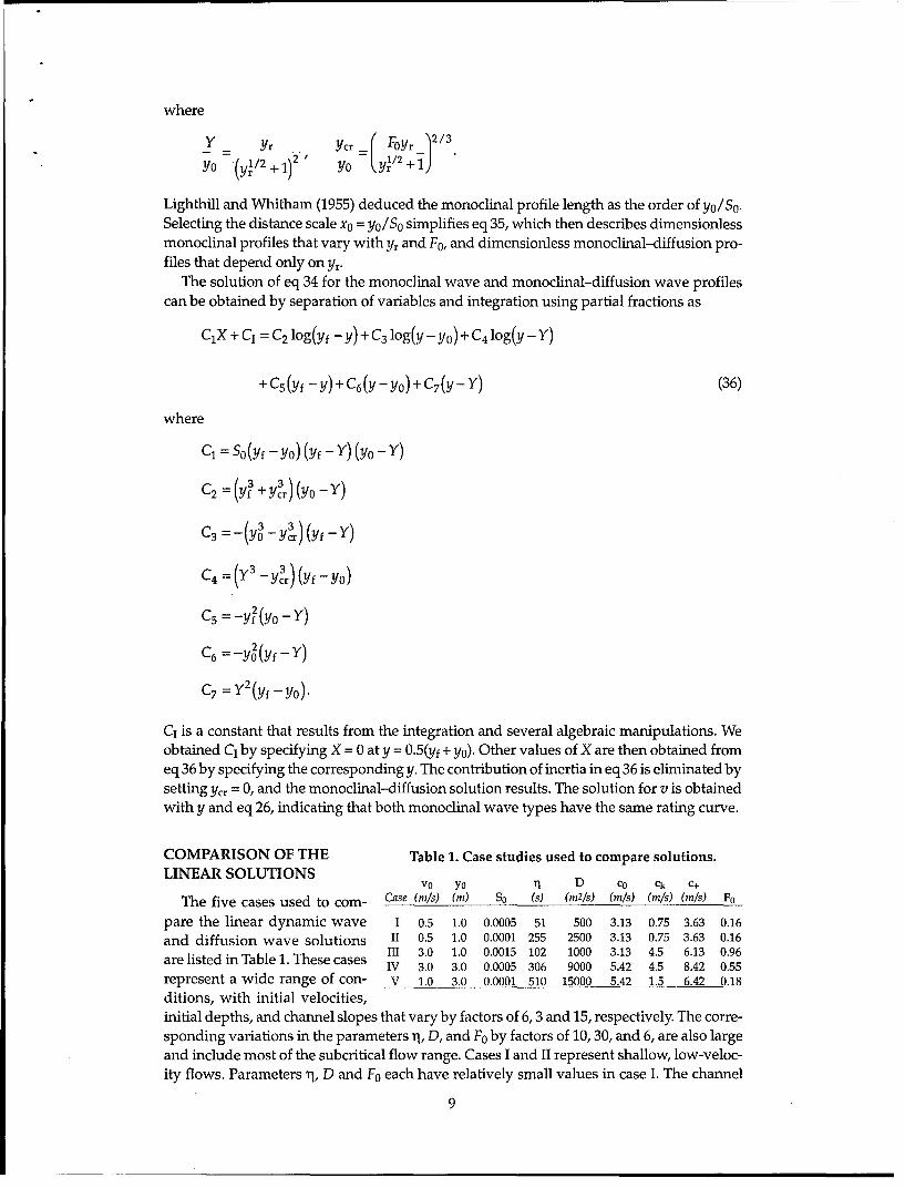
Lighthill and Whitham (1955) deduced the monoclinal profile length as the order of yo/So.Selecting the distance scale x0 = yo/So simplifies eq 35, which then describes dimensionlessmonoclinal profiles that vary with Yr and F0, and dimensionless monoclinal-diffusion pro-files that depend only on Yr

The solution of eq 34 for the monoclinal wave and monoclinal-diffusion wave profilescan be obtained by separation of variables and integration using partial fractions as

C1X + CI = C2 1og(yf -y) + C3 1og(y - Yo) + C4 1og(y -Y)

+Cs(Yf -Y)+C 6 (y-Yo)+C7 (y- Y) (36)

where

C1 = SO(Yf- Y0)(Yf- Y)(Yo - Y)

c2 fy yr)(y0-Y)

c4=+ 3 _Y3 )(Yfyo)3- - )

C5 =-y(yo-Y)

C6 = _y2 (yf_y)

C7 =y 2 (yf - YO)

CI is a constant that results from the integration and several algebraic manipulations. Weobtained CI by specifying X = 0 at y = 0.5(yf + yo). Other values of X are then obtained fromeq 36 by specifying the corresponding y. The contribution of inertia in eq 36 is eliminated bysetting Ycr = 0, and the monoclinal-diffusion solution results. The solution for v is obtainedwith y and eq 26, indicating that both monoclinal wave types have the same rating curve.

COMPARISON OF THE Table 1. Case studies used to compare solutions.LINEAR SOLUTIONS v0 yo r• D co Ck c+

The five cases used to com- Case (mis) (i) SO (s) (m2/s) (m/s) (mis) (mis) Fo

pare the linear dynamic wave I 0.5 1.0 0.0005 51 500 3.13 0.75 3.63 0.16

and diffusion wave solutions II 0.5 1.0 0.0001 255 2500 3.13 0.75 3.63 0.16III 3.0 1.0 0.0015 102 1000 3.13 4.5 6.13 0.96IV 3.0 3.0 0.0005 306 9000 5.42 4.5 8.42 0.55

represent a wide range of con- V 1.0 3.0 0.0001 510 15000 5.42 1.5 6.42 0.18

ditions, with initial velocities,initial depths, and channel slopes that vary by factors of 6, 3 and 15, respectively. The corre-sponding variations in the parameters T, D, and F0 by factors of 10, 30, and 6, are also largeand include most of the subcritical flow range. Cases I and II represent shallow, low-veloc-ity flows. Parameters il, D and F0 each have relatively small values in case I. The channel

9

slope for case II is decreased relative to case I, while other parameters remain unchanged,corresponding to significantly increased i1 and D, with constant F0. Case III is a shallowhigh velocity flow with channel slope and velocity increased relative to the first two cases.Parameters il and D are near those of the first case, but F0 is at the high end of the range.Case IV represents a deeper and higher velocity flow than case I at an equal channel slope,corresponding to large Tj and D, with a midrange F0.Finally, the flow in case V is deep andrelatively slow with the highest T1 and D, and F0 near that of cases I and II.

Dimensionless profile celerities of selected points (4) = 0.1, 0.3, 0.5,0.7,0.9) were obtainedwith eq 17 and 23 for dynamic waves and diffusion waves, respectively, and results for allcases are presented in Figure 2. In early time, the leading edge of the diffusion wave profilemoves downstream at a celerity that initially exceeds and later is less than the dynamicwave celerity c,. The dynamic wave and diffusion wave profile celerities of all points con-verge toward each other and the kinematic wave celerity with time. At the midpoint 4) = 0.5both profile celerities rapidly approach the kinematic wave celerity and then remain con-stant. Smaller 0) profile celerities remain higher than those of larger 4, and diffusion contin-ues beyond 30 km in all cases.

In case I the discrepancies between diffusion wave and dynamic wave profile celerities

Case I Case 1I- Diffusion Diffusion

- Dynanric Dynamic

0.1

0.3

-I .

020 30 10 20 30x (krn) x (km)

1.6 Case 111 1.6 Case III- Diffusion Modified Diffusion

- - -ya -10 ---- Dynarc

1.2 0. 1 .2 0.3

0.7

0.4 0.4 -

0 10 20 30 10 20 30x(km) x (krn)

-\Case IV - Case Y

Figure 2. Dimensionless celerities of selected linear diffusion wave and dynamic wave profile pointsfor all cases plus case III with the modified inertial diusion coefficient. Note the changes in the

celerity scale between panels.

10

are minor at all points after 1 km of travel distance. Initial differences between the profilecelerities in case II occur as a result of the shock in the dynamic wave solution for 0 up to

0.5, and some differences persist for 5 km downstream. Similar profile celerity disagree-ment is also evident in case III, but celerity convergence after shock attenuation is inexact,with a slightly larger range remaining in the diffusion wave solution. With the modifiedinertial diffusion coefficient (eq 12) all case III diffusion wave and dynamic wave profilecelerities converge by 6 km, the distance for shock attenuation below 0 = 0.1. The large D in

case IV causes leading edge diffusion wave profile celerities to greatly exceed the dynamic

wave celerity. The shock persists for 17 km downstream, again delaying profile celerityagreement. The profile celerity change in case IV with the inertial diffusion coefficient wasnegligible. The celerity comparisons for case V are similar to those of case IV, with larger

initial dimensionless profile celerities in both solutions, and celerity agreement at all pointsfollowing shock attenuation at 17 km.

Traces on the x-t plane of selected wave profile points in Figure 3 help to visualize the

effects of profile celerity differences. The time scales used for each case are related by thekinematic wave celerities given in Table 1. The dynamic wave f from the origin at t = 0,

termed the dynamic forerunner by Stoker (1957), carries the initial shock downstream at aconstant celerity c,. A positive value of F(x,t,o) immediately behind the forerunner indi-cates that a given q is on the forerunner. The 0-traces that successively separate from the

Case 11-iDiffusion

Diffusi-°n,-o

7' -00

th ynm orrnerffr l asspuscseIIwihte o e nrtaDiffusion coeiffiient Nifsote

S~Case III

Figure 3. Traces on the x-t plane of selected linear diff-usion wave and dynamic wave profile points andthe dynamic forerunner f for all cases plus case III with the modified inertial diffusion coefficient. Note

the changes in the time scale between panels.

11

dynamic forerunner indicate a progressively diminishing shock amplitude. Afterward,f sep-arates from the profile and no longer contributes to the solution. Overall, the x-t traces indi-cate general agreement between the dynamic wave and diffusion wave solutions followingattenuation of the initial shock.

The case I traces of all corresponding dynamic wave and diffusion wave profile points areessentially identical. The dynamic forerunnerf in case I begins to separate from the profile inthe first 5 km, and leads by increasing distances farther downstream. At early time in case IIthe diffusion profile celerity of the leading edge exceeds that off, causing minor differencesbetween the traces. These differences disappear about 5 km from the origin, and thereafter thetraces of all points are identical. The forerunner and profile in case II progressively separatebeyond 10 km from the origin. The high F0 in case III reduces the rate of spread of the dynamicprofile, causing the diffusion traces of the front half to lead and of the back half to lag thedynamic traces, and these trends persist. With the inertial diffusion coefficient the traces incase III agree closely beyond 8 km, and the profile progressively separates fromf beyond 15km. In case IV a shock amplitude of 0.1 is carried by the forerunner for 16 km, withfseparat-ing from the profile beyond 25 km. Excess profile spreading in the diffusion solution, causedby initial celerity differences and high diffusion coefficient, persists throughout and was notgreatly improved by the inertial diffusion coefficient. The case V dynamic wave and diffusionwave traces compare similarly to those of case IV, except that differences higher on the profiledo not persist.

We can compare dynamic wave and diffusion wave profiles through time on a single figureby using a moving x-coordinate system with origin at 4) = 0.5. Comparisons of these origin x-values through time (Xdyn, Xdif) are given in Figure 4. The origin traces of the dynamic wavemodel were similar for cases with the same kinematic wave celerity. The absolute value of thedifference in origin position between the dynamic wave and diffusion wave models was al-

600 E1.05 8 0 l li I I i i iII I 1,5 i i i I i I I ~ I I 1i l I

600

IzS400X X 0.90

"n" 0.85 -200

, 0.8 I 1t I , l , i 0I I)0.4 1.0 10 40"t (S( 10-3)

0.4 1.0 10 40 .t (sxl0-3)

X"

100 0.01Xd(km) 19 =1I .0

1.0 0.001

0,4' 0.00040.4 1.0 10 40 0.4 1.0 10 40t (Sx 10 -3) t(sx10-3)

Figure 4. Comparison between origin positions of the moving coordinate system in the linear diffusionwave (xdif) and dynamic wave (xdyn) models for all cases.

12

ways less than 800 m, and diminished to less than 4 % of Xdyn after 1 hour. The ratio of theseorigin positions rapidly approached 1 from below in all cases. Larger diffusion coefficientscorrespond to larger absolute differences in origin position early and generally larger ratiodifferences from 1.

Dynamic wave and diffusion wave profiles at selected times are compared in the movingcoordinate system in Figure 5. The dynamic wave solution includes the initial shock on theforerunner. At early time the leading edge of the diffusion profile always precedes that of thedynamic profile by a distance that increases with D or 1i and the Froude number. The profilesin case I rapidly converge and are nearly identical after 1200 s. In case II the shock front ispreserved for a longer time, and the profiles converge by 10,800 s. With high F0 in case III theprofiles tend to converge after the shock diminishes, but the dynamic wave profile retainsmore steepness than the diffusion wave profile. Case III profiles with the inertial diffusioncoefficient are nearly identical after 3600 s. In case IV the shock persists for a longer time, andprofile convergence requires more than 10,800 s. The minor differences in profile steepnessremaining at large times can be minimized with the inertial diffusion coefficient. The case Vprofile comparisons are similar to those of case IV, but with a low Froude number the inertialdiffusion coefficient is not needed for agreement at large times. Monoclinal wave profiles of

3600 Case 1 036 0 -1000 Case 11

0.8 10, 00 Diffusion 0.8 -10,800 - DiffuSIon36,000 - 36,000 - Dynanic

0.6 m_ , 0.6 -

0.4 - .

0.0.40.2 0.2 -

0 r I I I I f I-10 -8 -6 -4 -2 0 2 4 6 8 10 20 -16 -12 -8 -4 0 4 a 12 16 20

x (kM) x (KMn)

1.0 -- _ --- ----- I, Ca 111 1.0 12001 48 s --- DiffusDllo•300 1111 -. 'Case III3 M- DysnarIc - 36,00 1, 0 0 1 - 480 - Modified Diffusiono.8 . 0.8- - "- -_ ' \ \ \l-- ,,•-

00 -Dynam

0.6 - - 0.6 "

0.4 -- -- 0.4 -

0.2 0.2 -. • ••

I II I -

-20 -16 -12 -8 -4 0 4 8 12 16 20 0-20 -16 -12 -8 -4 0 4 8 12 16 20x (km) x (kM)

0. t- -- 0: 5 \ I•' I c- 0v 1 480 scase lY Case V

0.Diffusion Diffusion- DynaniC- DyTnarr~c

-30 -20 -10 0 10 20 30 - -30 -20 -10 0 10 20 30 40x (krn) x (km)

Figure 5. Linear diffusion wave and dynamic wave profiles and small-amplitude monoclinal wave profile m for allcases plus case III with the modified inertial diffusion coefficient. Note the changes in the distance scale between panels.

13

amplitude 0 .1yo, representing fully diffused linear wave profiles at large times, are alsogiven for each case in Figure 5. The most prominent feature of these solutions is the lowprofile slope, and the extended time indicated for the linear wave to attain this profile. Onlythe higher Froude number linear profiles at 36,000 s even approach the small-amplitudemonoclinal profiles.

ANALYSIS OF THE MONOCLINAL SOLUTIONS

The numerator of the depth gradient in eq 34 does not change sign along the profile, buta sign change in the denominator can result from the presence of inertia. This sign changeindicates a monoclinal wave profile that turns back upstream, becomes unstable, and formsa shock. In contrast, the monoclinal-diffusion profile cannot become unstable because Ycr isnot present. Initial monoclinal wave instability occurs at the toe of the profile when thedenominator goes to zero, and

Y=Yo = Ycr )1 3. (37)

Following Hunt (1987) we evaluate the stability limit eq 37 using eq 28, and after somealgebra, the depth ratio across the wave Yr is obtained as a function of F0

Yr _ 1 +,( +FO)J •2 (38)

The depth ratio range of stable monoclinal wave profiles decreases as Froude number in-creases toward 2. Conversely F0 can be obtained as a function of Yr with eq 35 as

F0 = (39)Yr

The stability limit in eq 37, evaluated using eq 26, yields U = vo+co as the maximumprofile celerity prior to instability. The range of stable profile celerities, bounded below bythe celerity of lower-order kinematic waves and bounded above by the celerity of higher-order dynamic waves, can be written in dimensionless form as

1 < 1 + 1. (40)Ck 31 Fo

Dimensionless profile celerity and overrun discharge given in Figure 6 increase continu-ously with wave amplitude from lower limits of 1 and 0.5, respectively, at Yr = Yf/Yo = 1. Theupper limits are indicated for selected values of F0 by dots that follow from eq 40.

The difference between the monoclinal and monoclinal-diffusion solutions can be para-meterized by considering the bracketed term in eq 33 rewritten using dimensionless vari-ables

(F0Yr21- B2 = 1_(Ycr3 =~1_ (r ) (41)

gy 3 [(RYr -- 1)9 + 1] 3

where dimensionless depth 9, defined analogously to ý in eq 13, varies between 0 and 1.

14

5-- a.

0FO 0.20. 5

Ck 3 -B

- .0.4

0.5

0 10 20 30 40 50

1.4 I I I I 1.1b. 30 5 0.9 BY

030

/ .1.1

0,9

ok 1.25 B1.2 - 0.8 0Vo

0 Y,

1.5 -0.7

2.0 -0.61.75

" i I i I ' 1!. 05

1.0 1.4 1.0 2.2 2.6 3.0Yf/Yo

Figure 6. Dimensionless monoclinal profile celerity and overrun dischargeas a function of depth ratio. The stable profile range spans a depth ratio rangefrom 1 to an upper bound, indicated by the dots, that decreases as the Froudenumber increases. Panel b is an expanded view of the shaded area of panel a.

For monoclinal-diffusion waves eq 41 has a value of 1, and the deviation from 1 indicatesthe relative importance of inertia. The same cases analyzed for linear waves are used todepict monoclinal waves, with time deleted from the parameters considered and depthratio across the wave representing amplitude added. Evaluations of eq 41 for each case arepresented in Figure 7 as a function of Yr for selected values of y, all with limit 1 - Fo2/ 4 at yr= 1. At low Froude numbers the part of the profile affected by inertia is very close to leadingedge (small 9), and then only when depth ratios are large. Differences between monoclinaland monoclinal-diffusion profiles near the leading edge increase with Yr and F0.Negativevalues of eq 41 indicate that the profile point y is located on a shock. Cases I and II have acalculated stability limit of Yr = 51, where the dimensionless shock amplitude is smallerthan 0.001. In case III with high F0 much more of the profile is affected by inertia, and largershocks occur at relatively small depth ratios. Case IV is intermediate between these condi-tions, and case V is similar to cases I and II.

Monoclinal and monoclinal-diffusion dimensionless depth profiles for case I, presentedin Figure 8, are in exact agreement except for the leading edge at Yr = 50, where the diffusionsolution leads. The front half of these profiles shorten and steepen as Yr increases to 10. AtYr = 50 the wave front lengthens, and the steepest portion continues forward to the leadingedge. The profile comparisons and trends for case II in Figure 9 are identical to those of caseI, except that profile lengths are significantly increased as a result of much higher diffusion.Case III, depicted in Figure 10, has monoclinal and monoclinal-diffusion profiles that pro-gressively separate below a dimensionless depth of about 0.4. The leading edge of thesteeper monoclinal profile lags behind that of the diffusion profile. At Yr = 5, outside thestable profile range, overrun of the leading edge of the monoclinal profile indicates shockformation up to a dimensionless depth of about 0.1. Case IV in Figure 11 is qualitatively

15

1.0 .

0.8 V .

0..0

0.4=

022

0.0.5 0.5 025

0.8 .1

0. =0.0010.

0.2j~ 0.0011 00.20

0.0 IOr 0 10 20 30 40 0 12 3 4 7

-.0 - 0.5 0.25ffsio

I0 1

x~0.1

0.Cas.01

0.12

~~Figure 8. Cvlain fe 1ase mounoclina andet moocia-ioffusletdiesionlprfil s atth twothmonclna pofdist eanc scal e oeth hnes forth depth ratios rangin between 1.1nadl50

0.16

Case It

0.8 -- Monoclnal- Monocliral-diffusion

- 50

-120 -80 -40 0 40 80 120x (km)

Case 11

O.- Monocilnal-MonocdinaI-diffuslori

10

-60 -40 -20 0 20 40 80x (km)

Figure 9. Case II monoclinal and monoclinal-diff-usion profiles at twodistance scales for depth ratios ranging between 1. 1 and 50.

- Case III

0.8- Monocinal-Monoclinal-ciffusion

0.6-m

Figur 10. Cae1.mnc1nladmnclnldfuio rflsa

tw0itne clsfrdet aisragn2ewen11ad517.

Case IV

-- Monoc¢inal. Monoclinal-diffusion

0.4-

I II

0.2-- .2.0 -

-30 -40 -20 0 20 40 60x(kmn)

Case 1Y --

--8 M oclInal

Figure 1 C oonoclnal-diffusion

p l

0.6-

t n fe 10.

0.2 w. A .0

10 -------

-0 - 20 - 10 0 10O 20 30x (kin)

Figure 11. Case IV monoclinal and monoclinal-diflusion profiles attwo distance scales for depth ratios ranging between 1.1 and 10.

similar to case III with distance scales substantially increased. At y, = 2 the profiles begin to

separate at a dimensionless depth of about 0.3, and an overrun of the leading edge occurs atYr = 10 up to a dimensionless depth of 0.03. Case V, presented in Figure 12, is qualitativelysimilar to cases I and I1 except that the largest diffusion coefficient produces the longest pro-files of all the cases.

General results from these comparisons are that monoclinal and monoclinal-diffusionprofiles agree for all values of Yr with F0 • 0.2, and that profile length increases with i1 or D.At small F0 the depth ratio needed to produce a shock is large, and the shock height andoverrun distance of the leading edge are small. These results agree with the Lighthill andWhitham (1955) contention that dynamic waves are subordinated at "well subcritical"Froude numbers. As F0 increases the monoclinal waves differ over a larger portion of theprofile, shocks occur at smaller depth ratios and their dimensionless amplitudes increase,and for a given ir the profile length decreases. General dimensionless monoclinal-diffusionprofiles for each depth ratio are given in Figure 13 as a function of t, and include the profilesof all cases as indicated by eq 35. Similar dimensionless monoclinal profile plots in Figure 14are almost as well-behaved, but differences near the leading edge occur for each Yr due totheir F0 dependence.

Steady flow rating curves relate river stage or mean depth at a given location to a uniquedischarge. The governing equation for linear waves holds with either v or y as the depen-dent variable, indicating a fixed steady flow rating. In unsteady flow the discharge relatingto a given stage generally varies from that for steady flow, depending on the rate of rise orfall of the hydrograph. We will develop and compare dimensionless monoclinal wave andsteady flow ratings. Using eq 26, an equation for the monoclinal wave unit discharge can bewritten in terms of depth and depth ratio as

18

Case V

0.8- - Monocldnal- Monoclinal-diffuslon

0.4--Y. .

-300 -200 -100 0 100 200 300

FiguresCase V o

1.0 I I I i I I

00. Monolinal- M onoclinal-Mfuslon

0.6

0.4-0

.00.2-0

0.0 I

- 150 100 -50 0 50 100 150x (km)

Figure 12. Case V monoclinal and monoclinal-diff-usion profiles attwo distance scales for depth ratios ranging between 1.1 and 35.

1.0 I

Yr- 2.

0.8 Yr= 50

0.6

0.4

0.2

F u 13Yr= 1.1

o

0.0 1 _ _ I I 1 y 2-60 -40 -10 201 40 60

1.01

0,8~ ~ ~Yr -- 2=-- y

0.6

0.4 ,

Yr 10

0.2

\5 Y yr=2Figure 13. General monoclinal-0. o , , , Yr= s diffusion profiles at two dimen-

-20 -10 0 10 20 sionless distance scales for depthS~ratios ranging between 1.1 and 50.

19

o Case I, II, V0.8 a Case III

-Case IV

0.6

0.4

0.2Yr- 1.1 Yr 5

0.0 I I 1-60 -40 -20 0 20 40 60 -20 -10 0 10 20Y 1.

1.0 i ' _ I I i I i

0.8

0.6

0.4

02 yr= 2 Yr= 10

0.0 I II-20 -10 0 10 20 -20 -10 0 10 20

Figure 14. Monoclinal profiles for all cases at two dimensionless distance scales for depthratios ranging between 1.1 and 10.

q _ vy (y/yo)(y 1/2 1yr(y /2y (412

qo voYo (Yr - )(42)

Defining dimensionless unit discharge with the same form as dimensionless depth, eq 2becomes

(43)

independent of the depth ratio. Using the Chezy equation we obtain a corresponding rela-tionship for dimensionless unit discharge in steady flow conditions as a function of depthratio

[(Yr - 1)y• + 1]3/2 _ 1 (44)qsteady = y 3r/2 -1

In the linear wave limit as Yr approaches 1, the rating curves represented by eq 43 and 44 areidentical. These rating curves, given in Figure 15, indicate that for a given dimensionlessdepth as Yr increases the monoclinal wave unit discharge also increases relative to that forsteady flow.

Froude number and energy gradient along a linear wave are unchanged from those ofthe initial steady flow. Large amplitude monoclinal waves with discharges along the pro-file that greatly exceed those of steady flow at comparable depths can have significantlylarger Sf and F. We define E - Sf/So, and with the Chezy equation and eq 26 obtain

E (viv0 ) 2 (F 2 (Yr/21)+1]2

Y/YO F [( -1)y+1]3(45)20

St.y 0ses 5

0.6-

0.4-

0.2

U 0.2 0.4 0.60.10

q

Figure 15. Dimensionless monoclinal and steady state rating curves fordepth ratios ranging between 2 and 50.

Figure 16 gives E as a function of 9 for selected values of Yr. The maximum E increases withYr and moves from near the midpoint of the profile toward the leading edge. Conversely,Figure 17 gives E as a function of Yr for selected values of Y. At small Yr the largest E islocated near the midpoint of the profile. As Yr increases E approaches a constant starting atthe midpoint of the profile and progressing toward the leading edge. At large depth ratiosE is inversely proportional to Y, increasing toward the leading edge.

a.

Yr 50

7 35

6

5

420

3 5 2See 'b -

2

10 YrlO b.

6.33

1 .5-

2.75

2.0

I I 1 1.1 1 -0 0.2 0.4 0.6 0.8 1.0

Figure 16. Energy gradient and Froude number parameter E along the monocli-nal wave profile for selected depth ratios. Panel b is an expanded view of the shadedarea in panel a.

21

a.

See "by 0.05

7-

6 -.

4- 0.2

See "b' 0.253 0

0.42

0.5

0 10 20 30 40 50

b.

0.2

2.0 - 0.3

E 0.4

0.5

1.5

2 4 6 8 10Yr

Figure 17. Energy gradient and Froude number parameter E as a function ofdepth ratio for selected dimensionless depths along the profile. Panel b is an ex-panded view of the shaded area in panel a.

0.5

0.4 -7

0.3 6

-5 Emax

0.2 4

-30.1

010 20 30 40 50

Yr

Figure 18. Dimensionless depth and corresponding maximum E as functions of depth ratio.

The dimensionless depth corresponding to maximum E for a given depth ratio can be

obtained by differentiating eq 45 with respect to 9 and setting the result to zero as

- 2 32=- 3/2 -1" (46)

Yr -1 yr2

22

The maximum E is then obtained by substituting eq 46 into 45 and simplifying

E4 =( y 3 / 2 _ 1 )

3

Emax (47)2 7 Yr(Yr -) 2 (yl/2-)

The location and value of Emax are given in Figure 18. Emax increases nearly linearly overthe Yr range, and its location rapidly approaches the leading edge as Yr increases from 1.Both energy gradient and Froude number vary continuously along the monoclinal waveprofile, with amplitudes proportional to Yr. Froude numbers that exceed 1 can occur onstable profiles when F0 is large, as in case III.

CONCLUSIONS

The presence or absence of the inertia terms distinguishes dynamic wave and diffusion

wave models of unsteady river flow. Analytical solutions of the linear dynamic wave anddiffusion wave equations were compared for a small instantaneous increase from an initialsteady, uniform flow condition throughout the channel to a higher steady flow velocity,and depth at the upstream boundary. The comparison used case studies that represented awide range of flow depth, velocity, channel slope, and wave diffusion coefficient, andspanned the range of subcritical Froude numbers. Analytical solutions were also obtainedfor nonlinear monoclinal wave and monoclinal-diffusion wave equations, and compari-sons were again made using the same case studies with a wide range of wave amplitudes.The linear solution comparisons focused on the evolution of the dynamic wave and diffu-sion wave profiles with time and distance, while the nonlinear solution comparisons inves-tigated the effects of wave amplitude and persistent inertia.

The linear solution comparisons included the celerity and the trace on the x-t plane ofselected points from the wave profile, and the complete dynamic and diffusion profiles atselected times. The initial shock traveled downstream with the dynamic forerunner at c+,the maximum celerity in subcritical flow. A limitation of the diffusion wave solution ispremature replacement of this shock by a profile having a range of point celerities thatexceed c+ near the leading edge. The diffusion wave and dynamic wave profiles remaindistinct until after the shock attenuates and their profile celerities converge. In cases wherethe Froude number approaches 1, this convergence requires a diffusion coefficient cor-rected for inertia. Points near the leading edge of each profile travel faster than those higheron the profile, causing diffusion. These differences diminish over time and distance, and alldynamic and diffusion profile celerities asymptotically approach that of a kinematic wave.General agreement of the linear diffusion wave and dynamic wave solutions after attenua-tion of the shock is indicated in all cases by common profile celerities and x-t traces, and byprofile covergence with time. The role of the characteristics in the linear solution becomesnegligible following shock attenuation at time and distance scales that increase with both iiand the Froude number.

The analysis of the nonlinear monoclinal wave solutions linked important inertial effectsat large time with increasing Froude number. As F0 increases corresponding monoclinaland monoclinal-diffusion profiles separate near the leading edge, and these differencesincrease with wave amplitude. Monoclinal profile instability occurs at higher F0, but mono-clinal-diffusion profiles are always stable. General dimensionless monoclinal-diffusionprofiles exist for each depth ratio with distance scaled by yo/So, but monoclinal profilesdeviate from these general profiles at higher F0 . Several effects of wave amplitude on mon-oclinal waves were also identified. The celerity of a small-amplitude monoclinal waveequals that of a kinematic wave, and it increases continuously from this lower limit with

23

wave amplitude. The steepness near the front of the monoclinal wave profile and the differ-ence between monoclinal and steady flow or linear wave rating curves both increase asamplitude increases. The energy gradient and Froude number at all points along the profilealso increase with wave amplitude, and the location of the maximum shifts continuouslytoward the leading edge.

LITERATURE CITED

Agsorn, S., and J.C.I. Dooge (1991) Numerical experiments on the monoclinal rising wave.Journal of Hydrology, 124: 293-306.Carslaw, H.S., and J.C. Jaeger (1959) Conduction of Heat in Solids. Oxford: Oxford UniversityPress, 2nd ed., p. 387-388.Chow, V.T. (1959) Open Channel Hydraulics. New York: McGraw-Hill, p. 528-537.Dooge, J.C.I. (1973) Linear theory of hydrologic systems. USDA Agricultural Research Ser-vice, Washington, D.C., Technical Bulletin no.1468.Dooge, J.C.I., and B.M. Harley (1967) Linear routing in uniform open channels, In Proceed-ings of the International Hydrology Symposium, Fort Collins, Colorado, 6-8 September, vol. 1, p.57-63.Ferrick, M.G. (1985) Analysis of river wave types. Water Resources Research, 21: 209-220.Ferrick, M.G., J. Bilmes, and S.E. Long (1984) Modeling rapidly varied flow in tailwaters.Water Resources Research, 20: 271-289.Hayami, S. (1951) On the propagation of flood waves. Disaster Prevention Research Insti-tute, Kyoto University, Japan, Bulletin no. 1.Henderson, EM. (1966) Open Channel Flow. New York: Macmillan Company.Hunt, B. (1987) A perturbation solution of the flood-routing problem. Journal of HydraulicResearch, 25: 215-234.Kundzewicz, Z.W., and J.C.I. Dooge (1989) Attenuation and phase shift in linear flood rout-ing. Hydrological Sciences Journal, 34: 21-40.Lighthill, M.J., and G.B. Whitham (1955) On kinematic waves. I: Flood movement in longrivers. Proceedings of the Royal Society (London) (A), 229: 281-316.Mahmood, K., and V. Yevjevich (Ed.) (1975) Unsteady Flow in Open Channels. Fort Collins,Colorado: Water Resources Publications, vol. I, p. 29-62.Mendoza, C. (1995) Discussion of "Identification of reservoir flood-wave models" by V.P.Singh and J. Li. Journal of Hydraulic Research, 33: 420-422.Menendez, A.N. (1993) The asymptotic wave form for a space-limited perturbation in openchannels. Journal of Hydraulic Research, 31: 635-650.Menendez, A.N., and R. Norscini (1982) Spectrum of shallow water waves: an analysis. Jour-nal of the Hydraulics Division, ASCE, 108: 75-94.Ponce, V.M., and D.B. Simons (1977) Shallow wave propagation in open channel flow. Jour-nal of the Hydraulics Division, ASCE, 103: 1461-1476.Ponce, V.M., R.M. Li, and D.B. Simons (1978) Applicability of kinematic and diffusion mod-els. Journal of the Hydraulics Division, ASCE, 104: 353-360.Press, W.H., S.A. Teukolsky, W.T. Vetterling, and B.P. Flannery (1992) Numerical Recipes inFORTRAN. New York: Cambridge University Press, second edition, p. 123-155,229-233.Stoker, J.J. (1957) Water Waves. New York: Wiley-Interscience, p. 482-509.Whitham, G.B. (1974) Linear and Nonlinear waves. New York: Wiley-Interscience, p. 87-91,339-350.Woolhiser, D.A., and J.A. Liggett (1967) Unsteady one-dimensional flow over a plane-Therising hydrograph. Water Resources Research, 3(3), 753-771.

24

REPORT DOCUMENTATION PAGE I Form ApprovedlI 0MB No. 0704-0188

Public reporting burden for this collection of information is estimated to average 1 hour per response, including the time for reviewing instructions, searching existing data sources, gathe-ri-ng 7ndmaintaining the data needed, and completing and reviewing the collection of information. Send comments regarding this burden estimate or any other aspect of this collection of information,including suggest ion for reducing this burden, to Washington Headquarters Services, Directorate for Information Operations and Reports, 1215 Jefferson Davis Highway, Suite 1204, Arlington,VA 22202-4302, and to the Office of Management and Budget, Paperwork Reduction Project (0704-0188), Washington, DC 20503.

1. AGENCY USE ONLY (Leave blank) 2. REPORT DATE 3. REPORT TYPE AND DATES COVERED

IJanuary 1998 I______________4. TITLE AND SUBTITLE S. FUNDING NUMBERS

Analysis of Linear and Monoclinal River Wave Solutions DA Project DT08CWIS Project 7VC103

6. AUTHORS

Michael G. Ferrick and Nicholas J. Goodman

7. PERFORMING ORGANIZATION NAME(S) AND ADDRESS(ES) 8. PERFORMING ORGANIZATIONREPORT NUMBER

U.S. Army Cold Regions Research and Engineering Laboratory72 Lyme Road CRREL Report 98-1Hanover, New Hampshire 03755-1290

9. SPONSORING/MONITORING AGENCY NAME(S) AND ADDRESS(ES) 10. SPONSORING/MONITORINGAGENCY REPORT NUMBER

Office of the Chief of EngineersWashington, D.C. 20314-1000

11. SUPPLEMENTARY NOTES For conversion of SI units to non-SI units of measurement consult Standard Practice for Use of theInternational System of Units (SI), ASTM Standard E380-93, published by the American Society for Testing and Materials,1916 Race St., Philadelphia, Pa. 19103.

12a. DISTRIBUTION/AVAILABILITY STATEMENT 12b. DISTRIBUTION CODE

Approved for public release; distribution is unlimited.

Available from NTIS, Springfield, Virginia 22161.

13. ABSTRACT (Maximum 200 words)Linear dynamic wave and diffusion wave analytical solutions are obtained for a small, abrupt flow increase froman initial to a higher steady flow. Equations for the celerities of points along the wave profiles are developed fromthe solutions and related to the kinematic wave and dynamic wave celerities. The linear solutions are comparedsystematically in a series of case studies to evaluate the differences caused by inertia. These comparisons use thecelerities of selected profile points, the paths of these points on the x-t plane, and complete profiles at selectedtimes, indicating general agreement between the solutions. Initial diffusion wave inaccuracies persist over rela-tively short time and distance scales that increase with both the wave diffusion coefficient and Froude number.The nonlinear monoclinal wave solution parallels that of the linear dynamic wave but is applicable to arbitrarilylarge flow increases. As wave amplitude increases the monoclinal rating curve diverges from that for a linearwave, and the maximum Froude number and energy gradient along the profile increase and move toward theleading edge. A monoclinal-diffusion solution is developed for the diffusion wave equations, and dynamic wave-diffusion wave comparisons are made over a range of amplitudes with the same case studies used for linearwaves. General dimensionless monoclinal-diffusion profiles exist for each depth ratio across the wave, while cor-responding monoclinal wave profiles exhibit minor, case-specific Froude number dependence. Inertial effects onthe monoclinal profiles occur near the leading edge, increase with the wave amplitude and Froude number, andare responsible for the differences between the dimensionless profiles. ____________

14. SUBJECT TERMS 15. NUMBER OF PAGESAnalytical solutions Flood routing River waves 30Diffusion wave Linear waves Unsteady flow 16. PRICE CODEDynamic wave Monoclinal waves

17. SECURITY CLASSIFICATION 18. SECURITY CLASSIFICATION 19. SECURITY CLASSIFICATION 20. LIMITATION OF ABSTRACTOF REPORT OF THIS PAGE OF ABSTRACT

UNCLASSIFIED UNCLASSIFIED UNCLASSIFIED ULINSIN 7540-01-280-5500 Standard Form 298 (Rev. 2-89)

Prescribed by ANSI Std. Z39-1 8298-1 02