Embed Size (px)
Citation preview
ANALYSIS OF MOVING MESH PARTIAL DIFFERENTIALEQUATIONS WITH SPATIAL SMOOTHING∗
WEIZHANG HUANG† AND ROBERT D. RUSSELL‡
SIAM J. NUMER. ANAL. c© 1997 Society for Industrial and Applied MathematicsVol. 34, No. 3, pp. 1106–1126, June 1997 013
Abstract. Two moving mesh partial differential equations (MMPDEs) with spatial smoothingare derived based upon the equidistribution principle. This smoothing technique is motivated by therobust moving mesh method of Dorfi and Drury [J. Comput. Phys., 69 (1987), pp. 175–195]. It isshown that under weak conditions the basic property of no node-crossing is preserved by the spatialsmoothing, and a local quasi-uniformity property of the coordinate transformations determined bythese MMPDEs is proven. It is also shown that, discretizing the MMPDEs using centered finitedifferences, these basic properties are preserved.
Key words. moving mesh PDE, spatial smoothing
AMS subject classifications. 65M50, 65L50, 65N50
PII. S0036142993256441
1. Introduction. For the numerical solution of time-dependent PDEs whichinvolve large solution variations, a variety of moving mesh methods have been shown togain significant improvements in accuracy and efficiency over conventional fixed meshmethods (e.g., see [GDM81], [AF86], [DD87], [FVZ90], [HGH91], and [HRR94b]). Forthese methods, mesh equations which involve node speeds are employed to move amesh (generally having a fixed number of nodes) in such a way that the nodes remainconcentrated in regions of rapid variation of the solution. For almost all of them,mesh equations are represented in discrete form.
To facilitate a better understanding of moving mesh equations and to allow for abetter investigation of their basic properties, several continuous moving mesh equa-tions (MMPDEs) based upon the equidistribution principle have recently been de-rived in [HRR94a]. Some basic properties, such as stability and the potential fornode-crossing, are also analyzed. While the MMPDEs are derived in such a waythat temporal mesh smoothing occurs, a spatial mesh smoothing is also generallynecessary, and it is employed when developing practical moving mesh methods basedupon these MMPDEs in [HRR94b]. Since the accuracy and error in the solutionmay depend upon the type of discretization, the quality of the mesh, the treatmentof boundary conditions, etc., there is generally no simple relationship between thesmoothness of the mesh and the error (cf. [VR92]). Nevertheless, for most problemsand most discretization methods, abrupt variations in the mesh will cause a deterio-ration in the convergence rate and an increase in the error [MTW85]. Moreover, mostdiscrete approximations of spatial differential operators have much larger conditionnumbers on an abruptly varying mesh than they do on a gradually varying one (e.g.,see [SHR96]), and these ill-conditioned approximations may result in stiffness in thetime integration for time-dependent problems. It is thus not surprising that mesh
∗Received by the editors September 30, 1993; accepted for publication (in revised form) September12, 1995. This work was supported by the Natural Science and Engineering Research Council ofCanada grant OGP-0008781.
http://www.siam.org/journals/sinum/34-3/25644.html†Department of Mathematics and Statistics, Simon Fraser University, Burnaby B.C. V5A 1S6,
Canada. Current address: Department of Mathematics, 405 Snow Hall, University of Kansas,Lawrence, KS 66045 ([email protected]).
‡Department of Mathematics and Statistics, Simon Fraser University, Burnaby B.C. V5A 1S6,Canada ([email protected]).
1106
MOVING MESH PDEs WITH SPATIAL SMOOTHING 1107
quality has become an increasingly important issue in the field of mesh generationand mesh adaption [MTW85].
The objective of the paper is to introduce and analyze a natural spatial smoothingfor the MMPDEs. The spatial smoothing technique is partially motivated by therobust moving mesh method of Dorfi and Drury [DD87] and by the enlighteninganalysis of it in [VBFZ89]. The spatial smoothing is shown to inherit the no node-crossing property of the unsmoothed methods and to produce a locally quasi-uniformcoordinate transformation (with discrete form corresponding to the well-known localquasi-uniformity property [KN82], which provides a good measure of the smoothnessquality of a mesh in one dimension).
An outline of this paper is as follows. In section 2 the MMPDEs with spatialsmoothing are derived. The spatial smoothing is incorporated into the mathematicalanalysis of the MMPDEs and some of their finite difference approximations in sections3 and 4, respectively. Two numerical examples are provided in section 5 to show thepreservation of the local quasi uniformity of the mesh. Section 6 contains conclusionsand comments.
2. Formulation of MMPDEs with spatial smoothing. We shall derive inthis section our basic MMPDEs which are based upon the equidistribution principleand which also have spatial smoothing.
Let x and ξ denote the physical and computational coordinates, respectively, bothof which are without loss of generality assumed to be the unit interval [0, 1]. A one-to-one coordinate transformation between these domains, which will be determinedby an MMPDE, is denoted by
x = x(ξ, t), ξ ∈ [0, 1](1)
with
x(0, t) = 0, x(1, t) = 1,(2)
where t denotes time. For a given monitor function M(x, t)(> 0) which provides somemeasure of the computational difficulty in the solution of the underlying physicaldifferential equations, the equidistribution principle can be expressed in differentialform (e.g., see [HRR94a]) as
∂
∂ξ
{M(x(ξ, t), t)
∂x
∂ξ(ξ, t)
}= 0.(3)
Given M(x, t) and an initial transformation x = x(ξ, 0), x = x(ξ, t) can be determinedfor t > 0 from (3) and the boundary conditions (2). Since the initial transformation isoften chosen as a very smooth function, such as the “uniform transformation” x(ξ, 0) =ξ, or as a function determined from M(x, 0), it is realistic to assume that its propertieslike smoothness are determined by M(x, t). However, for most problems which involvelarge solution variations, the monitor function is generally fairly nonsmooth in space,and some kind of smoothing of M(x, t) should be employed in (3) in order to makethe transformation smooth (see [VBFZ89], [FVZ90], and [HRR94b]). To do this weintroduce a PDE in ξ and t which involves an artificial diffusion term for smoothingM , viz., we define M to satisfy
M − λ−2∆M = M(4)
1108 WEIZHANG HUANG AND ROBERT D. RUSSELL
and the boundary conditions
∂M
∂ξ(0, t) =
∂M
∂ξ(1, t) = 0.(5)
Here, λ is a positive number and
∆ =∂2
∂ξ2 .(6)
Denoting by G the restriction of the operator I − λ−2∆ on the space of functionssatisfying the boundary conditions (5), the solution of (4) and (5) can be expressedby
M = G−1M.(7)
In the next section we show that G−1 exists and analyze the extra smoothness prop-erties of M . It is worth noting that the operator G and its inverse G−1 commute withthe time differentiation. Replacing M in (3) by M gives the “smoother” equidistri-bution principle
∂
∂ξ
{M(ξ, t)
∂x
∂ξ(ξ, t)
}= 0(8)
or
∂
∂ξ
{(G−1M)(ξ, t)
∂x
∂ξ(ξ, t)
}= 0.(9)
As discussed in [HRR94a], a quasi-static form like (9) is an idealized form ex-pressing exact equidistribution, and in practice it can produce nonsmooth trajectories.Mesh equations involving node speeds, or so-called MMPDEs, based upon (9) gener-ally produce much smoother mesh trajectories and are more suited for the numericalsolution of time-dependent problems. Following the approach in [HRR94a], we re-quire (9) to be satisfied at the later time t + τ (0 < τ � 1). Expanding the resultingequation in a Taylor series in this relaxation parameter τ and dropping higher-orderterms, we obtain
∂
∂ξ
{∂
∂t
(∂x
∂ξG−1M
)}= −1
τ
∂
∂ξ
{∂x
∂ξG−1M
}(10)
or
∂
∂ξ
{∂x
∂ξ
∂
∂t(G−1M) +
∂x
∂ξG−1M
}= −1
τ
∂
∂ξ
{∂x
∂ξG−1M
},(11)
where x denotes ∂x∂t |ξ fixed. In actual computation, the term ∂
∂t (G−1M) will be com-
plicated and difficult to compute. It may be argued [HRR94a] that it is reasonable todrop this term, giving the simplification
∂
∂ξ
{∂x
∂ξG−1M
}= −1
τ
∂
∂ξ
{∂x
∂ξG−1M
}.(12)
This can be regarded as a smooth version of MMPDE 4 in [HRR94a], and similararguments can be used to show that (10) is asymptotically stable in the sense thatits solution satisfies
∂
∂ξ
{∂x
∂ξG−1M
}(ξ, t) = e− t
τ∂
∂ξ
{∂x
∂ξG−1M
}(ξ, 0) .
MOVING MESH PDEs WITH SPATIAL SMOOTHING 1109
Although analogous stability properties have not as yet been proved for (12), numer-ical experiments indicate that its solution is stable and continues to approximatelyequidistribute the monitor function for all times if a relatively small value of τ is used(cf. [HRR94a]).
Thus, one way to obtain a mesh which is smooth in both space and time is tosolve
∂
∂ξ
{M
∂x
∂ξ
}= −1
τ
∂
∂ξ
{M
∂x
∂ξ
}(13)
and (4) together for x and M . However, in some respects it does not seem to be asuitable approach since an additional equation (4) is introduced for M , and it doesnot involve time derivatives. Thus, here we shall not consider this method further butintroduce an alternative method which is likely to be more efficient and appropriatefor time-dependent problems.
In (12), G−1 is an integral operator, and discretization produces a dense matrixsystem. To obtain an alternative form we integrate in ξ to give
(G−1M)(
∂x
∂ξ+
1τ
∂x
∂ξ
)= c(t),(14)
where c(t) is an integral constant, and rewrite this as
M = c(t)G
(1
∂x∂ξ + 1
τ∂x∂ξ
).(15)
Now, differentiating with respect to ξ, we obtain
∂
∂ξ
G
(1
∂x∂ξ + 1
τ∂x∂ξ
)M
= 0.(16)
Since G is defined on the space of functions satisfying (5), we require x = x(ξ, t) tosatisfy
∂
∂ξ
(1
∂x∂ξ + 1
τ∂x∂ξ
)= 0 at ξ = 0 and ξ = 1(17)
for all positive τ . If ∂x∂ξ > 0 (which will later be shown to be satisfied), then this is
equivalent to requiring
∂2x
∂ξ2 (0, t) =∂2x
∂ξ2 (1, t) = 0.(18)
Hence, x(ξ) can be determined by solving the smooth MMPDE in the form
∂
∂ξ
(I − λ−2∆)
(1
∂x∂ξ + 1
τ∂x∂ξ
)M
= 0(19)
together with the boundary conditions (2) and (18).
1110 WEIZHANG HUANG AND ROBERT D. RUSSELL
Alternatively, it is instructive to introduce the so-called concentration function
n(ξ, t) =1∂x∂ξ
(20)
and to derive a smooth MMPDE for x written in terms of n. If we assume that nn is
uniformly bounded for all ξ and t, then for small τ
1∂x∂ξ + 1
τ∂x∂ξ
= τn1− τn
n
= τn(1 + τn
n + · · ·)= τn + τ2n + O(τ3).
(21)
Substituting (21) into (16) and dropping higher-order terms gives
∂
∂ξ
{G(n + 1
τ n)M
}= 0,(22)
where the definition of G requires that n satisfy the boundary conditions
∂n
∂ξ(0, t) =
∂n
∂ξ(1, t) = 0.(23)
This MMPDE is
∂
∂ξ
{(I − λ−2∆)(n + 1
τ n)M
}= 0(24)
or, equivalently,
∂
∂ξ
(˙n
M
)= −1
τ
∂
∂ξ
(n
M
),(25)
where
n = Gn.(26)
Note that both (19) and (25) are fourth-order (in space) differential equations forx requiring four boundary conditions. As will be seen, a centered finite differencediscretization of (25) gives exactly the moving finite difference method developed byDorfi and Drury in [DD87] (see section 4). Indeed, their scheme provides the originalmotivation for our introducing smoothing with the diffusion term in (4). However, (25)(or (19)) is more general and useful due to its differential form, and it can be solvedby any of the standard numerical methods, such as a finite element, collocation, orspectral method. Furthermore, the role of τ is more transparent using this continuousMMPDE approach.
Notice that the MMPDE (25) is only slightly more complicated than the (non-smoothed) MMPDEs in [HRR94a]. In the same way that MMPDE6 is obtained fromMMPDE4 in [HRR94a], a simple alternative MMPDE can be obtained from (25) bytaking M = 1 on the left-hand side, giving
∂
∂ξ
(˙n)
= −1τ
∂
∂ξ
(n
M
).(27)
MOVING MESH PDEs WITH SPATIAL SMOOTHING 1111
The “smoothed” equidistribution principle (8) can be rewritten as
∂
∂ξ
(n
M
)= 0.(28)
Therefore, the right-hand side term
−1τ
∂
∂ξ
(n
M
)(29)
in (25) and (27) can be interpreted as a source for the mesh movement, as a stabi-lizing term, or as a mechanism to pull the mesh back toward equidistribution, in theanalogous manner to the nonsmooth MMPDE context in [HRR94a].
In actual computation, the MMPDE is normally discretized at N equally spacedpoints
ξi = ih, i = 0, 1, . . . , N,(30)
where h = 1N . Then, a mesh xi = x(ξi, t), i = 0, 1, . . . , N, is obtained by solving the
resulting discrete mesh equations.The spatial smoothing technique in [HRR94b] which uses a certain average of
monitor function values at 2p + 1 adjacent mesh points can be interpreted with ourapproach here. It is not difficult to see that if the value of λ is properly chosen, thisaverage is closely related to replacing G−1 by the approximation
I + λ−2∆ + (λ−2∆)2 + · · · + (λ−2∆)p(31)
and using centered differences to approximate ∆ (e.g., ∆Mi ≈ Mi+1−2Mi+Mi−1h2 ).
It is generally necessary that the mesh has no node-crossings and varies graduallyin space. The first condition is guaranteed if
xi+1(t) − xi(t) > 0, i = 0, 1, . . . , N − 1,(32)
and to satisfy the second condition the natural requirement is that the mesh be locallyquasi uniform, that is,
1K
≤ xi+1 − xi
xi − xi−1≤ K, i = 1, 2, . . . , N − 1,(33)
for some fixed constant K > 1. Continuous analogues of these are the so-called nonode-crossing condition (or mesh consistency condition)
∂x
∂ξ> 0(34)
and the local quasi-uniformity condition∣∣∣∣∣∂2x∂ξ2
∂x∂ξ
∣∣∣∣∣ ≤ λ(35)
for the mesh transformation.The discrete equivalent of (20) is
ni+ 12(t) =
h
xi+1(t) − xi(t).(36)
1112 WEIZHANG HUANG AND ROBERT D. RUSSELL
This is the familiar mesh concentration function used in [DD87] and frequently ap-pearing in the literature on moving mesh methods. In terms of the concentrationfunction n(ξ, t), no node-crossing and local quasi uniformity can be expressed by
n(ξ, t) > 0(37)
and ∣∣∣∣∣∂n∂ξ
n
∣∣∣∣∣ ≤ λ.(38)
In the next section, we shall show that the solutions of MMPDEs (19) and (25)have properties (34) and (35) or (37) and (38), respectively. After that, the finitedifference discretization of these MMPDEs will be shown to inherit these propertiesin the forms (32) and (33).
3. Analysis of MMPDEs. The spatial smoothing properties of the operatorG are described in the following simple lemma, whose proof is given for completeness.
LEMMA 3.1. Suppose that f(ξ) is a function defined on [0, 1] satisfying
0 < α ≤ f(ξ) ≤ β < ∞ for all ξ ∈ [0, 1].(39)
Then, the solution of{Gv ≡ (I − λ−2∆)v = f, 0 < ξ < 1,dvdξ (0) = dv
dξ (1) = 0(40)
exists for all λ > 0 (therefore, G has an inverse), and v(ξ) = G−1f has the followingproperties:
(i) v also satisfies
0 < α ≤ v(ξ) ≤ β < ∞ for all ξ ∈ [0, 1].
(ii) v satisfies the smoothness condition∣∣∣∣∣dvdξ
v
∣∣∣∣∣ ≤ λ.(41)
Proof. Letting w := dvdξ , (40) can be rewritten as{
dvdξ = w,dwdξ = λ2v − λ2f
(42)
with w(0) = w(1) = 0. Writing the solution of (42) in the form{v = c1(ξ)eλξ + c2(ξ)e−λξ,
w = λc1(ξ)eλξ − λc2(ξ)e−λξ(43)
leads to {eλξ dc1
dξ + e−λξ dc2dξ = 0,
eλξ dc1dξ − e−λξ dc2
dξ = −λf
MOVING MESH PDEs WITH SPATIAL SMOOTHING 1113
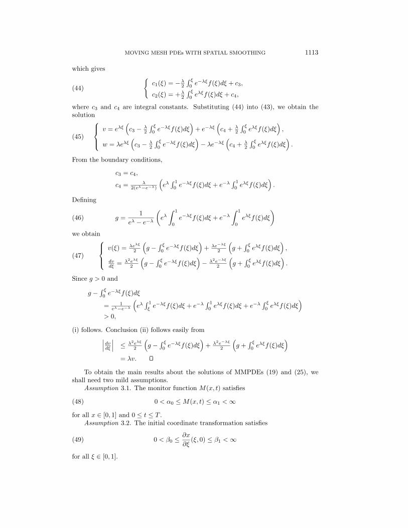
which gives {c1(ξ) = −λ
2
∫ ξ
0 e−λξf(ξ)dξ + c3,
c2(ξ) = +λ2
∫ ξ
0 eλξf(ξ)dξ + c4,(44)
where c3 and c4 are integral constants. Substituting (44) into (43), we obtain thesolution
v = eλξ(c3 − λ
2
∫ ξ
0 e−λξf(ξ)dξ)
+ e−λξ(c4 + λ
2
∫ ξ
0 eλξf(ξ)dξ)
,
w = λeλξ(c3 − λ
2
∫ ξ
0 e−λξf(ξ)dξ)
− λe−λξ(c4 + λ
2
∫ ξ
0 eλξf(ξ)dξ)
.(45)
From the boundary conditions,
c3 = c4,
c4 = λ2(eλ−e−λ)
(eλ∫ 10 e−λξf(ξ)dξ + e−λ
∫ 10 eλξf(ξ)dξ
).
Defining
g =1
eλ − e−λ
(eλ
∫ 1
0e−λξf(ξ)dξ + e−λ
∫ 1
0eλξf(ξ)dξ
)(46)
we obtainv(ξ) = λeλξ
2
(g − ∫ ξ
0 e−λξf(ξ)dξ)
+ λe−λξ
2
(g +
∫ ξ
0 eλξf(ξ)dξ)
,
dvdξ = λ2eλξ
2
(g − ∫ ξ
0 e−λξf(ξ)dξ)
− λ2e−λξ
2
(g +
∫ ξ
0 eλξf(ξ)dξ)
.(47)
Since g > 0 and
g − ∫ ξ
0 e−λξf(ξ)dξ
= 1eλ−e−λ
(eλ∫ 1
ξe−λξf(ξ)dξ + e−λ
∫ 10 eλξf(ξ)dξ + e−λ
∫ ξ
0 eλξf(ξ)dξ)
> 0,
(i) follows. Conclusion (ii) follows easily from∣∣∣dvdξ
∣∣∣ ≤ λ2eλξ
2
(g − ∫ ξ
0 e−λξf(ξ)dξ)
+ λ2e−λξ
2
(g +
∫ ξ
0 eλξf(ξ)dξ)
= λv.
To obtain the main results about the solutions of MMPDEs (19) and (25), weshall need two mild assumptions.
Assumption 3.1. The monitor function M(x, t) satisfies
0 < α0 ≤ M(x, t) ≤ α1 < ∞(48)
for all x ∈ [0, 1] and 0 ≤ t ≤ T .Assumption 3.2. The initial coordinate transformation satisfies
0 < β0 ≤ ∂x
∂ξ(ξ, 0) ≤ β1 < ∞(49)
for all ξ ∈ [0, 1].
1114 WEIZHANG HUANG AND ROBERT D. RUSSELL
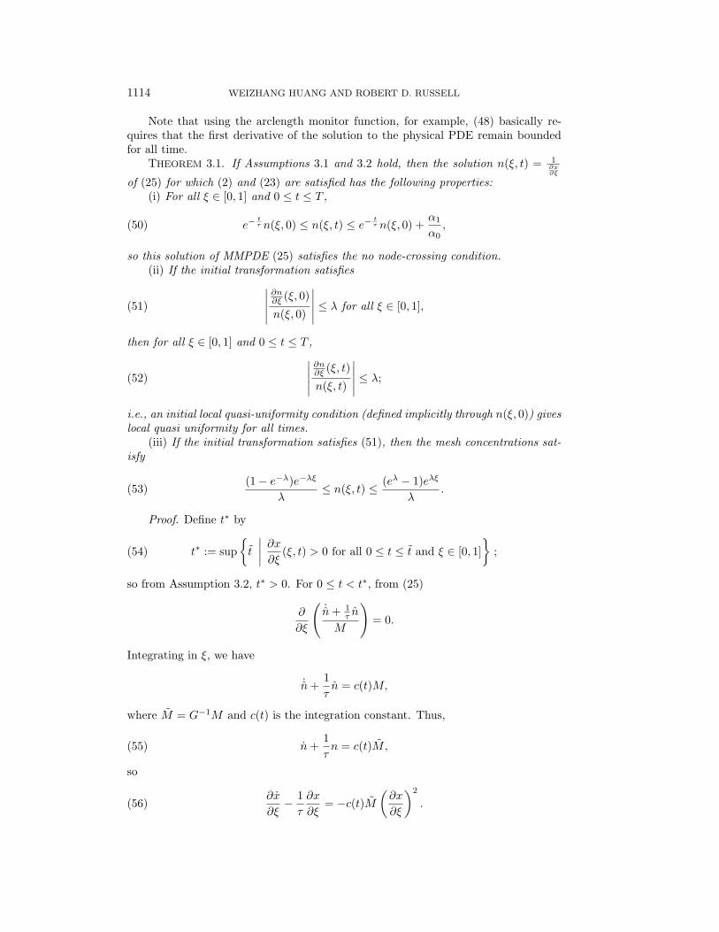
Note that using the arclength monitor function, for example, (48) basically re-quires that the first derivative of the solution to the physical PDE remain boundedfor all time.
THEOREM 3.1. If Assumptions 3.1 and 3.2 hold, then the solution n(ξ, t) = 1∂x∂ξ
of (25) for which (2) and (23) are satisfied has the following properties:(i) For all ξ ∈ [0, 1] and 0 ≤ t ≤ T ,
e− tτ n(ξ, 0) ≤ n(ξ, t) ≤ e− t
τ n(ξ, 0) +α1
α0,(50)
so this solution of MMPDE (25) satisfies the no node-crossing condition.(ii) If the initial transformation satisfies∣∣∣∣∣
∂n∂ξ (ξ, 0)
n(ξ, 0)
∣∣∣∣∣ ≤ λ for all ξ ∈ [0, 1],(51)
then for all ξ ∈ [0, 1] and 0 ≤ t ≤ T ,∣∣∣∣∣∂n∂ξ (ξ, t)
n(ξ, t)
∣∣∣∣∣ ≤ λ;(52)
i.e., an initial local quasi-uniformity condition (defined implicitly through n(ξ, 0)) giveslocal quasi uniformity for all times.
(iii) If the initial transformation satisfies (51), then the mesh concentrations sat-isfy
(1 − e−λ)e−λξ
λ≤ n(ξ, t) ≤ (eλ − 1)eλξ
λ.(53)
Proof. Define t∗ by
t∗ := sup{
t
∣∣∣∣ ∂x
∂ξ(ξ, t) > 0 for all 0 ≤ t ≤ t and ξ ∈ [0, 1]
};(54)
so from Assumption 3.2, t∗ > 0. For 0 ≤ t < t∗, from (25)
∂
∂ξ
(˙n + 1
τ n
M
)= 0.
Integrating in ξ, we have
˙n +1τ
n = c(t)M,
where M = G−1M and c(t) is the integration constant. Thus,
n +1τ
n = c(t)M,(55)
so
∂x
∂ξ− 1
τ
∂x
∂ξ= −c(t)M
(∂x
∂ξ
)2
.(56)

MOVING MESH PDEs WITH SPATIAL SMOOTHING 1115
From (2)
c(t) =
{τ
∫ 1
0M
(∂x
∂ξ
)2
dξ
}−1
.(57)
Since ∂x∂ξ > 0 for 0 ≤ t < t∗ and since M is a positive function satisfying (41) from
Lemma 3.1 and Assumption 3.1, we have
c(t) > 0 for 0 ≤ t < t∗.(58)
Integrating (55) in time gives
n(ξ, t) = e− tτ
(n(ξ, 0) +
∫ t
0c(t)e
tτ M(ξ, t)dt
),(59)
so that
n(ξ, t) ≥ e− tτ n(ξ, 0) for 0 ≤ t < t∗.(60)
The condition x(1, t) = 1 implies that∫ 1
0
1n(ξ, t)
dξ = 1;
hence, from (59) ∫ 1
0
dξ
n(ξ, 0) +∫ t
0 c(t)etτ M(ξ, t)dt
= e− tτ .(61)
From Assumptions 3.1 and 3.2 we have
e− tτ ≤ 1
1β1
+ α0∫ t
0 c(t)etτ dt
or
etτ
α0≥∫ t
0c(t)e
tτ dt.(62)
Now, (59) and (62) imply
n(ξ, t) ≤ e− tτ
(n(ξ, 0) + α1
∫ t
0 c(t)etτ dt)
≤ e− tτ
(n(ξ, 0) + α1e
tτ
α0
)= e− t
τ n(ξ, 0) + α1α0
.
Thus, we have obtained (50) for 0 ≤ t < t∗. From the continuity of n(ξ, t), (50) isalso true for t = t∗. If t∗ < T , then there exists at least one value of ξ, say ξ∗, suchthat ∂x
∂ξ (ξ∗, t∗) = 0. Since from (50) this is impossible, conclusion (i) holds.
1116 WEIZHANG HUANG AND ROBERT D. RUSSELL
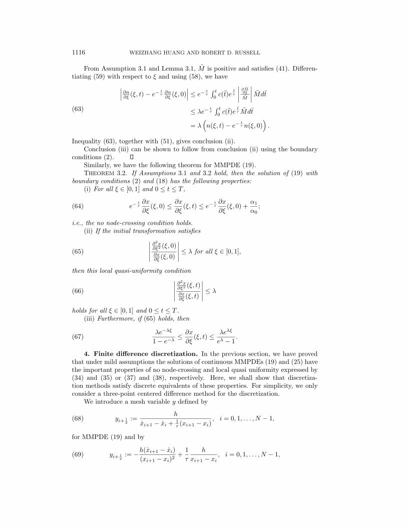
From Assumption 3.1 and Lemma 3.1, M is positive and satisfies (41). Differen-tiating (59) with respect to ξ and using (58), we have∣∣∣∂n
∂ξ (ξ, t) − e− tτ
∂n∂ξ (ξ, 0)
∣∣∣ ≤ e− tτ
∫ t
0 c(t)etτ
∣∣∣∣ ∂M∂ξ
M
∣∣∣∣ Mdt
≤ λe− tτ
∫ t
0 c(t)etτ Mdt
= λ(n(ξ, t) − e− t
τ n(ξ, 0))
.
(63)
Inequality (63), together with (51), gives conclusion (ii).Conclusion (iii) can be shown to follow from conclusion (ii) using the boundary
conditions (2).Similarly, we have the following theorem for MMPDE (19).THEOREM 3.2. If Assumptions 3.1 and 3.2 hold, then the solution of (19) with
boundary conditions (2) and (18) has the following properties:(i) For all ξ ∈ [0, 1] and 0 ≤ t ≤ T ,
e− tτ
∂x
∂ξ(ξ, 0) ≤ ∂x
∂ξ(ξ, t) ≤ e− t
τ∂x
∂ξ(ξ, 0) +
α1
α0;(64)
i.e., the no node-crossing condition holds.(ii) If the initial transformation satisfies∣∣∣∣∣
∂2x∂ξ2 (ξ, 0)∂x∂ξ (ξ, 0)
∣∣∣∣∣ ≤ λ for all ξ ∈ [0, 1],(65)
then this local quasi-uniformity condition∣∣∣∣∣∂2x∂ξ2 (ξ, t)∂x∂ξ (ξ, t)
∣∣∣∣∣ ≤ λ(66)
holds for all ξ ∈ [0, 1] and 0 ≤ t ≤ T .(iii) Furthermore, if (65) holds, then
λe−λξ
1 − e−λ≤ ∂x
∂ξ(ξ, t) ≤ λeλξ
eλ − 1.(67)
4. Finite difference discretization. In the previous section, we have provedthat under mild assumptions the solutions of continuous MMPDEs (19) and (25) havethe important properties of no node-crossing and local quasi uniformity expressed by(34) and (35) or (37) and (38), respectively. Here, we shall show that discretiza-tion methods satisfy discrete equivalents of these properties. For simplicity, we onlyconsider a three-point centered difference method for the discretization.
We introduce a mesh variable y defined by
yi+ 12
:=h
xi+1 − xi + 1τ (xi+1 − xi)
, i = 0, 1, . . . , N − 1,(68)
for MMPDE (19) and by
yi+ 12
:= −h(xi+1 − xi)(xi+1 − xi)2
+1τ
h
xi+1 − xi, i = 0, 1, . . . , N − 1,(69)
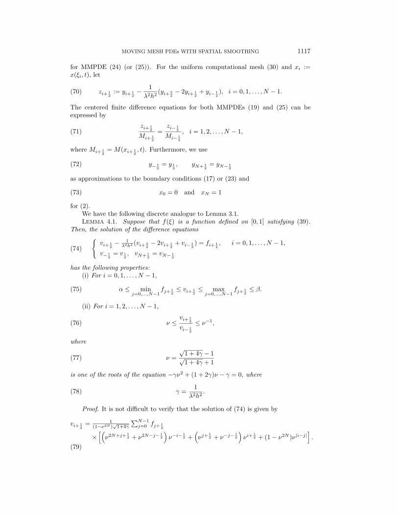
MOVING MESH PDEs WITH SPATIAL SMOOTHING 1117
for MMPDE (24) (or (25)). For the uniform computational mesh (30) and xi :=x(ξi, t), let
zi+ 12
:= yi+ 12
− 1λ2h2 (yi+ 3
2− 2yi+ 1
2+ yi− 1
2), i = 0, 1, . . . , N − 1.(70)
The centered finite difference equations for both MMPDEs (19) and (25) can beexpressed by
zi+ 12
Mi+ 12
=zi− 1
2
Mi− 12
, i = 1, 2, . . . , N − 1,(71)
where Mi+ 12
= M(xi+ 12, t). Furthermore, we use
y− 12
= y 12, yN+ 1
2= yN− 1
2(72)
as approximations to the boundary conditions (17) or (23) and
x0 = 0 and xN = 1(73)
for (2).We have the following discrete analogue to Lemma 3.1.LEMMA 4.1. Suppose that f(ξ) is a function defined on [0, 1] satisfying (39).
Then, the solution of the difference equations{vi+ 1
2− 1
λ2h2 (vi+ 32
− 2vi+ 12
+ vi− 12) = fi+ 1
2, i = 0, 1, . . . , N − 1,
v− 12
= v 12, vN+ 1
2= vN− 1
2
(74)
has the following properties:(i) For i = 0, 1, . . . , N − 1,
α ≤ minj=0,...,N−1
fj+ 12
≤ vi+ 12
≤ maxj=0,...,N−1
fj+ 12
≤ β.(75)
(ii) For i = 1, 2, . . . , N − 1,
ν ≤vi+ 1
2
vi− 12
≤ ν−1,(76)
where
ν =√
1 + 4γ − 1√1 + 4γ + 1
(77)
is one of the roots of the equation −γν2 + (1 + 2γ)ν − γ = 0, where
γ =1
λ2h2 .(78)
Proof. It is not difficult to verify that the solution of (74) is given by
vi+ 12
= 1(1−ν2N )
√1+4γ
∑N−1j=0 fj+ 1
2
×[(
ν2N+j+ 12 + ν2N−j− 1
2
)ν−i− 1
2 +(νj+ 1
2 + ν−j− 12
)νi+ 1
2 + (1 − ν2N )ν|i−j|].
(79)
1118 WEIZHANG HUANG AND ROBERT D. RUSSELL
The conclusions can now be easily obtained using (79) by noticing that
(80)
1(1−ν2N )
√1+4γ
×∑N−1j=0
[(ν2N+j+ 1
2 + ν2N−j− 12
)ν−i− 1
2 +(νj+ 1
2 + ν−j− 12
)νi+ 1
2 + (1 − ν2N )ν|i−j|]
= 1
for i = 0, 1, . . . , N − 1.The discrete analogue to Assumption 3.2 is as follows.Assumption 3.2′. The initial mesh satisfies
0 < β0 ≤ xi+1(0) − xi(0)h
≤ β1 < ∞, i = 0, 1, . . . , N − 1.(81)
Using Lemma 4.1 and following the approach in the proof of Theorem 3.1, thenext two theorems can be proven.
THEOREM 4.1. If Assumptions 3.1 and 3.2′ hold, then the solution of (71), (72),and (73) using (69) and (70) has the following properties:
(i) For i = 0, 1, . . . , N − 1 and 0 ≤ t ≤ T ,
e− tτ ni+ 1
2(0) ≤ ni+ 1
2(t) ≤ e− t
τ ni+ 12(0) +
α1
α0,(82)
where
ni+ 12(t) =
h
xi+1 − xi.(83)
(ii) If the initial mesh is locally quasi uniform
ν ≤ xi+1(0) − xi(0)xi(0) − xi−1(0)
≤ ν−1, i = 1, 2, . . . , N − 1,(84)
then the meshes are locally quasi uniform for all 0 ≤ t ≤ T , viz.,
ν ≤ xi+1(t) − xi(t)xi(t) − xi−1(t)
≤ ν−1, i = 1, 2, . . . , N − 1.(85)
(iii) If the initial mesh is locally quasi uniform, then
1 − ν
1 − νNνi ≤ xi+1(t) − xi(t) ≤ 1 − ν−1
1 − ν−Nν−i, i = 0, 1, . . . , N − 1.(86)
THEOREM 4.2. If Assumptions 3.1 and 3.2′ hold, then the solution of (71), (72),and (73) using (68) and (70) has the following properties:
(i) For i = 0, 1, . . . , N − 1 and 0 ≤ t ≤ T ,
e− tτ
xi+1(0) − xi(0)h
≤ xi+1(t) − xi(t)h
≤ e− tτ
xi+1(0) − xi(0)h
+α1
α0.(87)
(ii) If the initial mesh is locally quasi uniform
ν ≤ xi+1(0) − xi(0)xi(0) − xi−1(0)
≤ ν−1, i = 1, 2, . . . , N − 1,(88)

MOVING MESH PDEs WITH SPATIAL SMOOTHING 1119
then the meshes are locally quasi uniform for all 0 ≤ t ≤ T , viz.,
ν ≤ xi+1(t) − xi(t)xi(t) − xi−1(t)
≤ ν−1, i = 1, 2, . . . , N − 1.(89)
(iii) If the initial mesh is locally quasi uniform, then
1 − ν
1 − νNνi ≤ xi+1(t) − xi(t) ≤ 1 − ν−1
1 − ν−Nν−i, i = 0, 1, . . . , N − 1.(90)
We conclude this section with two observations about the discrete equations (71),(72), and (73) using (69) and (70). First, it is easy to verify that the mesh equationis exactly the one used in the Dorfi and Drury method if the parameter λ is chosensuch that γ = γ(1 + γ). Second, similar results to those in Theorem 4.1 have beenobtained in [VBFZ89]. The results in Theorem 4.1 are somewhat stronger than thosein [VBFZ89] since we obtain conclusions (ii) and (iii) without requiring that (71)be satisfied initially. More importantly, we interpret the method as a discretizationwhich inherits certain fundamental properties of a continuous transformation definedthrough the MMPDE (25).
5. Numerical examples. The capabilities of moving mesh methods have beenamply demonstrated elsewhere, so the MMPDEs are applied here to two simple prob-lems: a problem with solutions having derivative singularities and the well-knownBurgers equation with a smooth initial solution. The physical equations are firsttransformed into the computational coordinate and then discretized on the uniformmesh (30) by centered finite differences. The resulting finite difference equations, to-gether with the difference equations for MMPDE (19) or (25) (see (79)–(83)) and thecorresponding boundary conditions, constitute an ODE system which determines thephysical solution {ui(t)}N
i=0 and the mesh {xi(t)}Ni=0. The parameter λ in the spatial
smoothing process is determined by choosing γ in (78) as
γ = γ(γ + 1),(91)
where the values of γ will be given. Notice that γ = 0 corresponds to the case of nospatial smoothing.
This semidiscrete system is integrated in time by using the BDF code DASSL[Pet82], with approximate Jacobians being computed by the code internally via finitedifferences. For all computations the absolute and relative local time stepping errortolerances (in a root-mean-square norm) are taken as
atol = rtol = 10−7.(92)
The initial mesh is chosen as a uniform mesh and the value of the temporal smoothingparameter is taken as τ = 10−3. Note that DASSL normally requires {xi(0), ui(0)}and {xi(0), ui(0)} to be consistent. Since {xi(0), ui(0)} are unknown DASSL com-putes them internally. This often requires very small time stepsizes at the beginningof the time integration, and DASSL can sometimes fail altogether to find them. Inthe results presented, we measure the level of local quasi uniformity
L(t) = max{
xi+1(t) − xi(t)xi(t) − xi−1(t)
,xi(t) − xi−1(t)xi+1(t) − xi(t)
}(93)
and the level of global quasi uniformity
G(t) =max{xi+1(t) − xi(t)}min{xi+1(t) − xi(t)} .(94)

1120 WEIZHANG HUANG AND ROBERT D. RUSSELL
All computations are performed on a Silicon Graphics Indy workstation with adouble precision algorithm.
Example 5.1. A problem with solutions having derivative singularities. Our firstexample is
ut = uxx + f(x, t), x ∈ (0, 1), 0 < t ≤ 1,
u(0, t) = u(1, t) = 0, 0 < t ≤ 1,
u(x, 0) = 0, x ∈ [0, 1],(95)
where f(x, t) is chosen such that the exact solution is
u(x, t) = t(xα − x), α >12.(96)
The parameter α is assumed to be a noninteger number, so that the solution (96) hasa derivative singularity at x = 0, which models the singularity caused by corners of thedomain in two-dimensional problems. This type of singularity is thoroughly studiedin [GB86] for h, p, and h-p versions of the finite element method in one dimension, anda class of optimal meshes with respect to solution error in several norms is presented.
Interestingly, such optimal meshes can also be obtained using the equidistributionprinciple (3). Specifically, for the time-independent problem Carey and Dinh [CD85]show that if the monitor function is chosen as
M =[u(p+1)
]2/[2(p+1−m)+1],(97)
where the approximate solution u is a polynomial of degree p in each subinterval, thenthe solution error e is minimized in the Hm seminorm |•|m (where |e|2m :=
∫ 10 [e(m)]2dx)
and can be bounded by
|e|2m ≤ 1(πN)2(p+1−m)
1∫0
[u(p+1)]2
[ξ′]2(p+1−m) dx(1 + O(∆xmax)),(98)
where ξ′ denotes ∂ξ∂x . It is straightforward to show from (3) that the optimal coordinate
transformation (mesh) for the solution (96) is
x = ξ[2(p+1−m)+1]/[2α−2m+1],(99)
and for m = 1, (99) is precisely the so-called optimal radical mesh of Gui and Babuska[GB86].
The three-point centered finite difference approximation can be regarded as apolynomial approximation of degree p = 1 in x (cf. [CD85]). If the energy norm
|e|E(t) :=
1∫
0
∣∣∣∣ ∂e
∂x
∣∣∣∣2 dx
1/2
(100)
is used (i.e., m = 1), then the optimal monitor function is
M = [uxx]2/3,(101)
MOVING MESH PDEs WITH SPATIAL SMOOTHING 1121
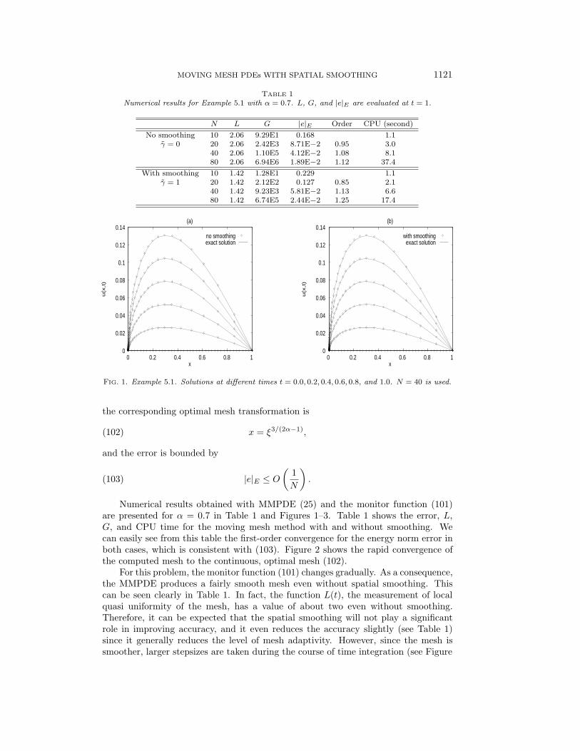
TABLE 1Numerical results for Example 5.1 with α = 0.7. L, G, and |e|E are evaluated at t = 1.
N L G |e|E Order CPU (second)No smoothing 10 2.06 9.29E1 0.168 1.1
γ = 0 20 2.06 2.42E3 8.71E−2 0.95 3.040 2.06 1.10E5 4.12E−2 1.08 8.180 2.06 6.94E6 1.89E−2 1.12 37.4
With smoothing 10 1.42 1.28E1 0.229 1.1γ = 1 20 1.42 2.12E2 0.127 0.85 2.1
40 1.42 9.23E3 5.81E−2 1.13 6.680 1.42 6.74E5 2.44E−2 1.25 17.4
0
0.02
0.04
0.06
0.08
0.1
0.12
0.14
0 0.2 0.4 0.6 0.8 1
u(x
,t)
x
(a)
no smoothingexact solution
0
0.02
0.04
0.06
0.08
0.1
0.12
0.14
0 0.2 0.4 0.6 0.8 1
u(x
,t)
x
(b)
with smoothingexact solution
FIG. 1. Example 5.1. Solutions at different times t = 0.0, 0.2, 0.4, 0.6, 0.8, and 1.0. N = 40 is used.
the corresponding optimal mesh transformation is
x = ξ3/(2α−1),(102)
and the error is bounded by
|e|E ≤ O
(1N
).(103)
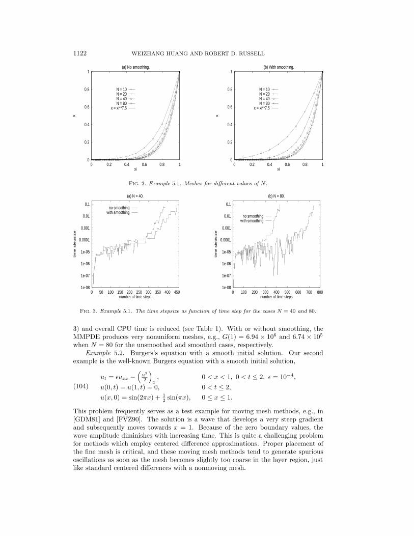
Numerical results obtained with MMPDE (25) and the monitor function (101)are presented for α = 0.7 in Table 1 and Figures 1–3. Table 1 shows the error, L,G, and CPU time for the moving mesh method with and without smoothing. Wecan easily see from this table the first-order convergence for the energy norm error inboth cases, which is consistent with (103). Figure 2 shows the rapid convergence ofthe computed mesh to the continuous, optimal mesh (102).
For this problem, the monitor function (101) changes gradually. As a consequence,the MMPDE produces a fairly smooth mesh even without spatial smoothing. Thiscan be seen clearly in Table 1. In fact, the function L(t), the measurement of localquasi uniformity of the mesh, has a value of about two even without smoothing.Therefore, it can be expected that the spatial smoothing will not play a significantrole in improving accuracy, and it even reduces the accuracy slightly (see Table 1)since it generally reduces the level of mesh adaptivity. However, since the mesh issmoother, larger stepsizes are taken during the course of time integration (see Figure
1122 WEIZHANG HUANG AND ROBERT D. RUSSELL
0
0.2
0.4
0.6
0.8
1
0 0.2 0.4 0.6 0.8 1xi
(a) No smoothing.
N = 10N = 20N = 40N = 80
x = xi**7.5
0
0.2
0.4
0.6
0.8
1
0 0.2 0.4 0.6 0.8 1
xx
xi
(b) With smoothing.
N = 10N = 20N = 40N = 80
x = xi**7.5
FIG. 2. Example 5.1. Meshes for different values of N .
1e-08
1e-07
1e-06
1e-05
0.0001
0.001
0.01
0.1
0 50 100 150 200 250 300 350 400 450
tim
e s
tep
siz
e
number of time steps
(a) N = 40.
no smoothingwith smoothing
1e-08
1e-07
1e-06
1e-05
0.0001
0.001
0.01
0.1
0 100 200 300 400 500 600 700 800
tim
e s
tep
siz
e
number of time steps
(b) N = 80.
no smoothingwith smoothing
FIG. 3. Example 5.1. The time stepsize as function of time step for the cases N = 40 and 80.
3) and overall CPU time is reduced (see Table 1). With or without smoothing, theMMPDE produces very nonuniform meshes, e.g., G(1) = 6.94 × 10⁶ and 6.74 × 10⁵
when N = 80 for the unsmoothed and smoothed cases, respectively.Example 5.2. Burgers’s equation with a smooth initial solution. Our second
example is the well-known Burgers equation with a smooth initial solution,
ut = εuxx −(
u2
2
)x
, 0 < x < 1, 0 < t ≤ 2, ε = 10−4,
u(0, t) = u(1, t) = 0, 0 < t ≤ 2,
u(x, 0) = sin(2πx) + 12 sin(πx), 0 ≤ x ≤ 1.
(104)
This problem frequently serves as a test example for moving mesh methods, e.g., in[GDM81] and [FVZ90]. The solution is a wave that develops a very steep gradientand subsequently moves towards x = 1. Because of the zero boundary values, thewave amplitude diminishes with increasing time. This is quite a challenging problemfor methods which employ centered difference approximations. Proper placement ofthe fine mesh is critical, and these moving mesh methods tend to generate spuriousoscillations as soon as the mesh becomes slightly too coarse in the layer region, justlike standard centered differences with a nonmoving mesh.
MOVING MESH PDEs WITH SPATIAL SMOOTHING 1123
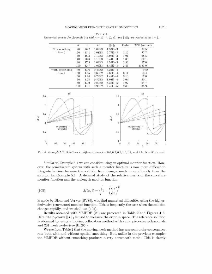
TABLE 2Numerical results for Example 5.2 with ε = 10−4. L, G, and ||e||1 are evaluated at t = 2.
N L G ||e||1 Order CPU (second)No smoothing 40 26.2 1.09E3 7.37E−3 32.5
γ = 0 50 31.1 1.08E3 5.77E−3 1.10 47.760 18.3 1.10E3 4.07E−3 1.91 68.570 20.6 1.10E3 3.44E−3 1.09 87.180 17.3 1.09E3 2.52E−3 2.33 97.0100 12.7 1.06E3 1.46E−3 2.45 1183.0
With smoothing 40 1.96 9.46E2 5.24E−4 9.58γ = 1 50 1.95 9.69E2 2.62E−4 3.11 13.4
60 1.94 9.79E2 1.48E−4 3.13 17.070 1.93 9.85E2 1.08E−4 2.04 20.180 1.92 9.89E2 8.36E−5 1.92 24.7100 1.91 9.93E2 4.40E−5 2.88 35.9
-1
-0.5
0
0.5
1
1.5
0 0.2 0.4 0.6 0.8 1
u(x
,t)
x
(a)
no smoothingref solution
-1
-0.5
0
0.5
1
1.5
0 0.2 0.4 0.6 0.8 1
u(x
,t)
x
(b)
with smoothingref solution
FIG. 4. Example 5.2. Solutions at different times t = 0.0, 0.2, 0.6, 1.0, 1.4, and 2.0. N = 80 is used.
Similar to Example 5.1 we can consider using an optimal monitor function. How-ever, the semidiscrete system with such a monitor function is now more difficult tointegrate in time because the solution here changes much more abruptly than thesolution for Example 5.1. A detailed study of the relative merits of the curvaturemonitor function and the arclength monitor function
M(x, t) =
√1 +
(∂u
∂x
)2
(105)
is made by Blom and Verwer [BV89], who find numerical difficulties using the higher-derivative (curvature) monitor function. This is frequently the case when the solutionchanges rapidly, and we shall use (105).
Results obtained with MMPDE (25) are presented in Table 2 and Figures 4–6.Here, the L1-norm || • ||1 is used to measure the error in space. The reference solutionis obtained by using a moving collocation method with cubic piecewise polynomialsand 201 mesh nodes (see [HR96]).
We see from Table 2 that the moving mesh method has a second-order convergencerate both with and without spatial smoothing. But, unlike in the previous example,the MMPDE without smoothing produces a very nonsmooth mesh. This is clearly
1124 WEIZHANG HUANG AND ROBERT D. RUSSELL
1
10
100
1000
0 0.2 0.4 0.6 0.8 1 1.2 1.4 1.6 1.8 2
L(t
)
t
(a)
no smoothingwith smoothing
1
10
100
1000
10000
0 0.2 0.4 0.6 0.8 1 1.2 1.4 1.6 1.8 2
G(t
)
t
(b)
no smoothingwith smoothing
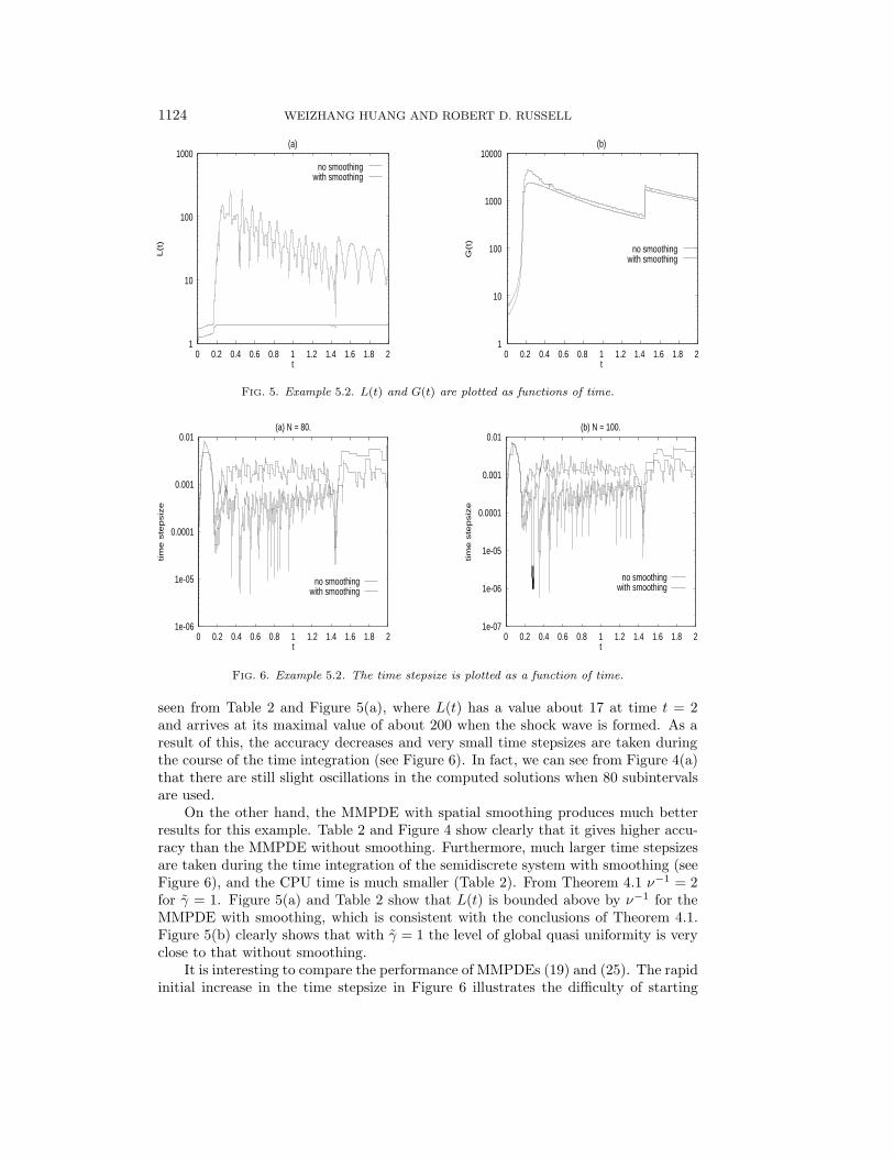
FIG. 5. Example 5.2. L(t) and G(t) are plotted as functions of time.
1e-06
1e-05
0.0001
0.001
0.01
0 0.2 0.4 0.6 0.8 1 1.2 1.4 1.6 1.8 2
tim
e s
tepsiz
e
t
(a) N = 80.
no smoothingwith smoothing
1e-07
1e-06
1e-05
0.0001
0.001
0.01
0 0.2 0.4 0.6 0.8 1 1.2 1.4 1.6 1.8 2
tim
e s
tepsiz
e
t
(b) N = 100.
no smoothingwith smoothing
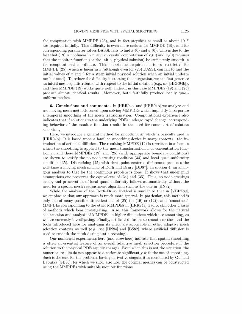
FIG. 6. Example 5.2. The time stepsize is plotted as a function of time.
seen from Table 2 and Figure 5(a), where L(t) has a value about 17 at time t = 2and arrives at its maximal value of about 200 when the shock wave is formed. As aresult of this, the accuracy decreases and very small time stepsizes are taken duringthe course of the time integration (see Figure 6). In fact, we can see from Figure 4(a)that there are still slight oscillations in the computed solutions when 80 subintervalsare used.
On the other hand, the MMPDE with spatial smoothing produces much betterresults for this example. Table 2 and Figure 4 show clearly that it gives higher accu-racy than the MMPDE without smoothing. Furthermore, much larger time stepsizesare taken during the time integration of the semidiscrete system with smoothing (seeFigure 6), and the CPU time is much smaller (Table 2). From Theorem 4.1 ν−1 = 2for γ = 1. Figure 5(a) and Table 2 show that L(t) is bounded above by ν−1 for theMMPDE with smoothing, which is consistent with the conclusions of Theorem 4.1.Figure 5(b) clearly shows that with γ = 1 the level of global quasi uniformity is veryclose to that without smoothing.
It is interesting to compare the performance of MMPDEs (19) and (25). The rapidinitial increase in the time stepsize in Figure 6 illustrates the difficulty of starting
MOVING MESH PDEs WITH SPATIAL SMOOTHING 1125
the computation with MMPDE (25), and in fact stepsizes as small as about 10−9
are required initially. This difficulty is even more serious for MMPDE (19), and forcorresponding parameter values DASSL fails to find xi(0) and ui(0). This is due to thefact that (19) is nonlinear in x, and successful computation of xi(0) and ui(0) requiresthat the monitor function (or the initial physical solution) be sufficiently smooth inthe computational coordinate. This smoothness requirement is less restrictive forMMPDE (25), which is linear in x (although even for (25) DASSL can fail to find theinitial values of x and u for a steep initial physical solution when an initial uniformmesh is used). To reduce the difficulty in starting the integration, we can first generatean initial mesh equidistributed with respect to the initial solution (e.g., see [HRR94b]),and then MMPDE (19) works quite well. Indeed, in this case MMPDEs (19) and (25)produce almost identical results. Moreover, both faithfully produce locally quasi-uniform meshes.
6. Conclusions and comments. In [HRR94a] and [HRR94b] we analyze anduse moving mesh methods based upon solving MMPDEs which implicitly incorporatea temporal smoothing of the mesh transformation. Computational experience alsoindicates that if solutions to the underlying PDEs undergo rapid change, correspond-ing behavior of the monitor function results in the need for some sort of solutionsmoothing.
Here, we introduce a general method for smoothing M which is basically used in[HRR94b]. It is based upon a familiar smoothing device in many contexts—the in-troduction of artificial diffusion. The resulting MMPDE (12) is rewritten in a form inwhich the smoothing is applied to the mesh transformation x or concentration func-tion n, and these MMPDEs (19) and (25) (with appropriate boundary conditions)are shown to satisfy the no node-crossing condition (34) and local quasi-uniformitycondition (35). Discretizing (25) with three-point centered differences produces thewell-known moving mesh scheme of Dorfi and Drury [DD87]. In section 4, an analo-gous analysis to that for the continuous problem is done. It shows that under mildassumptions one preserves the equivalents of (34) and (35). Thus, no node-crossingsoccur, and preservation of local quasi uniformity follows automatically without theneed for a special mesh readjustment algorithm such as the one in [KN82].
While the analysis of the Dorfi–Drury method is similar to that in [VBFZ89],we emphasize that our approach is much more general. In particular, this method isonly one of many possible discretizations of (25) (or (19) or (12)), and “smoothed”MMPDEs corresponding to the other MMPDEs in [HRR94a] lead to still other classesof methods which bear investigating. Also, this framework allows for the naturalconstruction and analysis of MMPDEs in higher dimensions which use smoothing, aswe are currently investigating. Finally, artificial diffusion to smooth meshes and thetools introduced here for analyzing its effect are applicable in other adaptive meshselection contexts as well (e.g., see [HN84] and [BS82], where artificial diffusion isused to smooth the mesh during static rezoning).
Our numerical experiments here (and elsewhere) indicate that spatial smoothingis often an essential feature of an overall adaptive mesh selection procedure if thesolution to the physical PDE rapidly changes. Even when this is not the situation, thenumerical results do not appear to deteriorate significantly with the use of smoothing.Such is the case for the problems having derivative singularities considered by Gui andBabuska [GB86], for which we show also how the optimal meshes can be constructedusing the MMPDEs with suitable monitor functions.
1126 WEIZHANG HUANG AND ROBERT D. RUSSELL
REFERENCES
[AF86] S. ADJERID AND J. E. FLAHERTY, A moving finite element method with error es-timation and refinement for one-dimensional time dependent partial differentialequations, SIAM J. Numer. Anal., 23 (1986), pp. 778–795.
[BS82] J. U. BRACKBILL AND J. S. SALTZMAN, Adaptive zoning for singular problems in twodimensions, J. Comput. Phys., 46 (1982), pp. 342–368.
[BV89] J. G. BLOM AND J. G. VERWER, On the Use of the Arclength and Curvature Monitorin a Moving Grid Method which is Based on the Method of Lines, Tech. reportNM-N8902, CWI, Amsterdam, 1989.
[CD85] G. F. CAREY AND H. T. DINH, Grading functions and mesh redistribution, SIAM J.Numer. Anal., 22 (1985), pp. 1028–1040.
[DD87] E. A. DORFI AND L. O’C. DRURY, Simple adaptive grids for 1-D initial value problems,J. Comput. Phys., 69 (1987), pp. 175–195.
[FVZ90] R. M. FURZELAND, J. G. VERWER, AND P. A. ZEGELING, A numerical study of threemoving grid methods for one-dimensional partial differential equations which arebased on the method of lines, J. Comput. Phys., 89 (1990), pp. 349–388.
[GB86] W. GUI AND I. BABUSKA, The h, p and h-p versions of the finite element method in onedimension, Part 1: The error analysis of the p-version; Part 2: The error analysisof the h and h-p version; Part 3: The adaptive h-p version, Numer. Math., 40(1986), pp. 577–612, pp. 613–657, pp. 659–683.
[GDM81] R. J. GELINAS, S. K. DOSS, AND K. MILLER, The moving finite element method:application to general partial differential equations with multiple large gradients,J. Comput. Phys., 40 (1981), pp. 202–249.
[HGH91] D. F. HAWKEN, J. J. GOTTLIEB, AND J. S. HANSEN, Review of some adaptive node-movement techniques in finite element and finite difference solutions of PDEs,J. Comput. Phys., 95 (1991), pp. 254–302.
[HN84] J. M. HYMAN AND M. J. NAUGHTON, Static rezone methods for tensor-product grids,in Proc. SIAM–AMS Conference on Large Scale Computation in Fluid Mechanics,SIAM, Philadelphia, PA, 1984.
[HR96] W. HUANG AND R. D. RUSSELL, A moving collocation method for the numerical so-lution of time dependent partial differential equations, Appl. Numer. Math., 20(1996), pp. 101–116.
[HRR94a] W. HUANG, Y. REN, AND R. D. RUSSELL, Moving mesh partial differential equations(MMPDEs) based on the equidistribution principle, SIAM J. Numer. Anal., 31(1994), pp. 709–730.
[HRR94b] W. HUANG, Y. REN, AND R. D. RUSSELL, Moving mesh methods based upon movingmesh partial differential equations, J. Comput. Phys., 113 (1994), pp. 279–290.
[KN82] J. KAUTSKY AND N. K. NICHOLS, Smooth regrading of discretized data, SIAM J. Sci.Statist. Comput., 3 (1982), pp. 145–159.
[MTW85] C. W. MASTIN, J. F. THOMPSON, AND Z. U. A. WARSI, Numerical Grid Generation:Foundations and Applications, Elsevier, New York, North–Holland, Amsterdam,1985.
[Pet82] L. R. PETZOLD, A Description of DASSL: A Differential/Algebraic System Solver,Tech. report SAND82-8637, Sandia Labs, Livermore, CA, 1982.
[SHR96] W. SUN, W. HUANG, AND R. D. RUSSELL, Finite difference preconditioning for solvingorthogonal collocation equations for boundary value problems, SIAM J. Numer.Anal., 33 (1996), pp. 2268–2285.
[VBFZ89] J. G. VERWER, J. G. BLOM, R. M. FURZELAND, AND P. A. ZEGELING, A movinggrid method for one-dimensional PDEs based on the method of lines, in AdaptiveMethods for Partial Differential Equations, J. E. Flaherty, P. J. Paslow, M. S.Shephard, and J. D. Vasilakis, eds., SIAM, Philadelphia, PA, 1989, pp. 160–175.
[VR92] A. E. P. VELDMON AND K. RINZEMA, Playing with nonuniform grids, J. Engrg. Math.,26 (1992), p. 119.