Embed Size (px)
Citation preview
Analysis of Network Quality Using Non-Intrusive Methods
from an End-User Perspective in LTE
Pedro Miguel Alves Venâncio
Thesis to obtain the Master of Science Degree in
Electrical and Computer Engineering
Supervisor: Prof. Luís Manuel de Jesus Sousa Correia
Examination Committee
Chairperson: Prof. Fernando Duarte Nunes
Supervisor: Prof. Luís Manuel de Jesus Sousa Correia
Members of the Committee: Prof. António José Castelo Branco Rodrigues
Eng. Chiara Bedini
June 2014

ii

iii
To my parents and sister

iv

v
Acknowledgements
Acknowledgements
First of all, I would like to thank Professor Luís M. Correia for giving me the opportunity to write this
thesis under his supervision, and for his guidance, discipline and constant support throughout the
development of this work. The experience was exceptional, allowing me to absorb priceless advices
from someone who has such a great academic and professional knowledge.
I would also like to thank Ericsson Portugal for allowing me to work inside a real telecommunications
business environment, and especially to Eng. Chiara Bedini for her constant assistance, guidance,
and technical support, that were essential throughout this journey.
To my fellow M.Sc. colleagues, for their companionship in the months we work together, and
especially to Pedro Ganço, Pedro Dinis and Bruno Pires for their motivation, advices, and inspired
conversations we shared during that time.
To all the members of Confraria, for their fellowship throughout the years, that taught me so much and
allowed me to become a better person. One could not ask for better friends. Also, to my friend Pedro
Lourenço for his tips and remarkable reviews, that helped me improve the quality of this thesis.
To my parents and sister, for their love, kindness and lifelong support. Without them I wouldn’t be
where I am today.
And to my girlfriend Rita, for her love and friendship all along these years, and for having the patience
to put up with her stubborn boyfriend in the times that he mostly needed.
For all of this and much more, I humbly say to all of you, thank you.

vi
vii
Abstract
Abstract
The main objective of this thesis was to analyse real network data, for both UMTS and LTE, and to fit
statistical distributions that enable the identification of worst sites within a network, regarding two
parameters: delay variation and packet loss. Both parameters were measured in the link between the
network site and its controller, which can be a microwave or an optical fibre one. Possible sources for
both these problems are also discussed along this work. The fitting of a statistical distribution to every
site, best representing the behaviour of each parameter, is an effort to predict their behaviour
throughout time. For this, a program in MATLAB© was developed, contains an algorithm to process
and evaluate data samples; in its core, it is a Chi-Square goodness-of-fit test, to ascertain which
distribution better fits the investigated parameters from a pre-defined group of distributions. For the
used scenario, it is concluded that one can model, with a significance level of 95%, 60% of the UMTS
NodeB’s delay variation via the Generalised Extreme Value distribution, while regarding packet loss,
56% can be model through the Log-logistic one. As for LTE, the Weibull and the Generalised Extreme
Value distributions describe best the behaviour of the same parameters, for 75% of all the sites
analysed for both cases. It is also found that link capacity and traffic volume are the aspects that have
more influence in the parameters studied.
Keywords
UMTS, LTE, Delay Variation, Packet Loss, Statistical Distributions, Goodness-of-Fit.
viii
Resumo
Resumo O principal objetivo desta tese consistiu em analisar dados reais de uma rede UMTS e LTE,
fornecidos pela Ericsson Portugal, e ajustar distribuições estatísticas que permitem identificar os
piores nós constituintes da rede relativamente a dois parâmetros: variação do atraso e perda de
pacotes. Possíveis fontes destes problemas são também discutidas. O ajuste de uma distribuição
estatística em cada nó, que melhor represente o andamento dos dois parâmetros, contribui para
prever os seus comportamentos ao longo do tempo. Para tal, foi desenvolvido um programa em
MATLAB© que contém um algoritmo para processar e avaliar as amostras dos dados, em que no seu
núcleo se encontra o teste Chi-Square Goodness-of-fit, para determinar de um pré-determinado grupo
de distribuições a que melhor represente os parâmetros investigados. Para o cenário usado, conclui-
se que, para UMTS é possível modelar a variação do atraso e a perda de pacotes através das
distribuições Generalised Extreme Value e Log-logistic, respetivamente em 60% e 56% das
situações, com uma confiança de 95%, enquanto que para o LTE, são as distribuições Weibull e
Generalised Extreme Value que melhor descrevem o comportamento dos mesmos parâmetros, em
75% das situações. Foi também concluído que a capacidade de ligação e o volume de trafego são os
aspetos que têm maior influência nos dois parâmetros estudados.
Palavras-chave
UMTS, LTE, Variação de Atraso, Perda de Pacotes, Distribuições Estatísticas, Goodness-of-Fit

ix
Table of Contents
Table of Contents
Acknowledgements ................................................................................. v
Abstract ................................................................................................. vii
Resumo ................................................................................................ viii
Table of Contents ................................................................................... ix
List of Figures ....................................................................................... xii
List of Tables ........................................................................................ xiv
List of Acronyms .................................................................................. xvi
List of Symbols ..................................................................................... xix
List of Software .................................................................................... xxii
1 Introduction ........................................................................................ 1
1.1 Overview ........................................................................................................ 2
1.2 Motivation and Contents ................................................................................ 5
2 Fundamental Concepts and State of the Art ....................................... 7
2.1 UMTS ............................................................................................................. 8
2.1.1 Network Architecture ...................................................................................................... 8
2.1.2 Radio Interface ............................................................................................................... 9
2.2 LTE .............................................................................................................. 10
2.2.1 Network Architecture .................................................................................................... 10
2.2.2 Radio Interface ............................................................................................................. 13
2.2.3 Coexistence with UMTS ............................................................................................... 15
2.3 Services and Applications ............................................................................ 17
2.4 Performance Monitoring............................................................................... 19
2.5 State of the Art ............................................................................................. 21
3 Performance Analysis Model ............................................................ 25
3.1 Performance Parameters ............................................................................. 26
x
3.2 Statistical Distributions ................................................................................. 27
3.3 Goodness-of-fit ............................................................................................ 31
3.4 Data Analysis Model .................................................................................... 34
3.5 Network Link Model ..................................................................................... 39
3.5.1 Optical Fibre Link Model .............................................................................................. 39
3.5.2 Microwave Link Model .................................................................................................. 41
4 Results Analysis ............................................................................... 45
4.1 Scenario ....................................................................................................... 46
4.2 UMTS Data Analysis .................................................................................... 48
4.2.1 Delay Variation ............................................................................................................. 48
4.2.2 Packet Loss .................................................................................................................. 55
4.2.3 UMTS Overview ........................................................................................................... 61
4.3 LTE Data Analysis ....................................................................................... 63
4.3.1 Delay Variation ............................................................................................................. 63
4.3.2 Packet Loss .................................................................................................................. 67
4.3.3 LTE Overview ............................................................................................................... 70
4.4 Network Link Model Analysis ....................................................................... 71
5 Conclusions ..................................................................................... 75
A Annex A - Statistical Distributions .................................................... 79
B Annex B - Chi-Square Distribution Table ......................................... 85
C Annex C - Chi-Square GoF Example Test ....................................... 87
D Annex D - Sites List (Confidential) ................................................... 91
E Annex E - Counters and KPI’s (Confidential) ................................... 93
F Annex F - UMTS List of Worst Sites ................................................. 95
F.1 Delay Variation ............................................................................................ 96
F.1.1 Weekday ...................................................................................................................... 96
F.1.2 Weekend ...................................................................................................................... 98
F.2 Packet Loss ............................................................................................... 100
F.2.1 Weekday .................................................................................................................... 101
F.2.2 Weekend .................................................................................................................... 103
G Annex G - UMTS Network Performance Maps (Confidential) ........ 107
H Annex H - LTE Network Performance Maps (Confidential) ............ 109
xi
References.......................................................................................... 111
xii
List of Figures
List of Figures Figure 1.1. Global mobile devices (extracted from [Cisc13]). .................................................................. 2 Figure 1.2. Evolution of 3GPP mobile communication standards (extracted from [SeTB11]). ................ 3 Figure 1.3. Predicted mobile data traffic (extracted from [Cisc13]). ......................................................... 3 Figure 1.4. Peak data rate in 3GPP standards (extracted from [HoTo09]). ............................................. 4 Figure 1.5. Evolution of LTE beyond LTE-A (extracted from [Eric13]). .................................................... 4 Figure 2.1. UMTS network architecture (extracted from [HoTo07]). ........................................................ 8 Figure 2.2. LTE network architecture (extracted from [AlLu11]). ...........................................................11 Figure 2.3. LTE time-domain structure (extracted from [DaPS11]). .......................................................14 Figure 2.4. Combined UMTS and LTE networks with 3G interfaces (adapted from [4GAm11]). ..........16 Figure 2.5. Combined UMTS and LTE networks with S interfaces (adapted from [4GAm11]). .............16 Figure 2.6. Mobile Backhaul for LTE and UMTS (adapted from [Eric13b]). ...........................................17 Figure 2.7. Service OAM and Link OAM (extracted from [Eric13d]). .....................................................21 Figure 3.1. Data analysis model – part 1. ...............................................................................................35 Figure 3.2. Data analysis model – part 2. ...............................................................................................36 Figure 3.3. Detailed Chi-Square test block. ............................................................................................37 Figure 3.4. Detailed distribution optimisation block. ...............................................................................38 Figure 3.5. Optical link model. ................................................................................................................40 Figure 3.6. Microwave link model. ..........................................................................................................42 Figure 4.1. Peak analysis for delay variation in UMTS. .........................................................................49 Figure 4.2. SiteID_8 over weekdays. .....................................................................................................50 Figure 4.3. SiteID_8 over the weekend. .................................................................................................50 Figure 4.4. Fitting distributions to SiteID_8’s delay variation data. ........................................................51 Figure 4.5. Resulting distributions considering mean value of its parameters. ......................................54 Figure 4.6. Peak analysis for packet loss in UMTS. ...............................................................................55 Figure 4.7. SiteID_25 behaviour during weekdays. ...............................................................................56 Figure 4.8. SiteID_82 behaviour during the weekend. ...........................................................................57 Figure 4.9. Overlapping of packet loss average values on all the worst sites, throughout the 24
hour day, for both scenarios. ........................................................................................57 Figure 4.10. Resulting distributions considering the average value of its parameters with
different number of hops, during the weekdays scenario. ............................................60 Figure 4.11. Resulting distributions considering the average value of its parameters with
different number of hops, during the weekend scenario...............................................61 Figure 4.12. Peak analysis for delay variation in LTE. ...........................................................................63 Figure 4.13. SiteID_107 delay variation, for LTE, during weekdays. .....................................................64 Figure 4.14. Fitting the distributions to SiteID_107’s delay variation data. ............................................65 Figure 4.15. Resulting distributions considering average value of its parameters. ................................67 Figure 4.16. LTE packet loss peaks during weekdays. ..........................................................................68 Figure 4.17. SiteID_107 packet loss values, for LTE, during weekdays. ...............................................68 Figure 4.18. SiteID_11 packet loss values, for LTE, during the weekend. ............................................69 Figure 4.19. All packet loss samples extracted, for all eNBs during weekdays. ....................................69 Figure A.1. Gamma distribution. .............................................................................................................80
xiii
Figure A.2. Generalised Extreme Value distribution. .............................................................................80 Figure A.3. Inverse Gaussian distribution. .............................................................................................80 Figure A.4. Logistic distribution. .............................................................................................................81 Figure A.5. Log-logistic distribution. .......................................................................................................81 Figure A.6. Log-normal distribution. .......................................................................................................81 Figure A.7. Nakagami distribution. .........................................................................................................82 Figure A.8. Rayleigh distribution. ...........................................................................................................82 Figure A.9. Rice distribution. ..................................................................................................................82 Figure A.10. Weibull distribution. ............................................................................................................83
Figure B.1. The shaded area is equal to φ for χ2 = χ1-φ2. ...................................................................86 Figure F.1. Behaviour of SiteID_8, in terms of delay variation, during weekdays. .................................96 Figure F.2. Behaviour of SiteID_51, in terms of delay variation, during weekdays. ...............................97 Figure F.3. Behaviour of SiteID_57, in terms of delay variation, during weekdays. ...............................97 Figure F.4. Behaviour of SiteID_59, in terms of delay variation, during weekdays. ...............................97 Figure F.5. Behaviour of SiteID_102, in terms of delay variation, during weekdays..............................98 Figure F.6. Behaviour of SiteID_8, in terms of delay variation, during the weekend. ............................99 Figure F.7. Behaviour of SiteID_51, in terms of delay variation, during the weekend. ..........................99 Figure F.8. Behaviour of SiteID_59, in terms of delay variation, during the weekend. ..........................99 Figure F.9. Behaviour of SiteID_107, in terms of delay variation, during the weekend. ......................100 Figure F.10. Behaviour of SiteID_57, in terms of delay variation, during the weekend. ......................100 Figure F.11. Behaviour of SiteID_25, in terms of packet loss, during weekdays. ................................102 Figure F.12. Behaviour of SiteID_34, in terms of packet loss, during weekdays. ................................102 Figure F.13. Behaviour of SiteID_75, in terms of packet loss, during weekdays. ................................102 Figure F.14. Behaviour of SiteID_82, in terms of packet loss, during weekdays. ................................103 Figure F.15. Behaviour of SiteID_29, in terms of packet loss, during weekdays. ................................103 Figure F.16. Behaviour of SiteID_82, in terms of packet loss, on the weekend. .................................104 Figure F.17. Behaviour of SiteID_81, in terms of packet loss, on the weekend. .................................105 Figure F.18. Behaviour of SiteID_34, in terms of packet loss, on the weekend. .................................105 Figure F.19. Behaviour of SiteID_75, in terms of packet loss, on the weekend. .................................105 Figure F.20. Behaviour of SiteID_29, in terms of packet loss, on the weekend. .................................106
xiv
List of Tables
List of Tables Table 2.1. Fundamental properties in 3GPP Release 99, 5, 6 and 7 (adapted from [Mart12]). ............10 Table 2.2. Service classes and requirements for UMTS QoS (extracted from [Corr13]). ......................18 Table 2.3. Standardised QoS Class Identifiers (extracted from [3GPP13b]). ........................................19 Table 3.1. Statistical distributions assessed – parameters and PDF [MatL14]. .....................................29 Table 3.2. Statistical distributions assessed – mean value and standard deviation [MatL14]. ..............30 Table 4.1. Number of sites analysed. .....................................................................................................46 Table 4.2. Number of sites with a specific number of hops....................................................................46 Table 4.3. Days evaluated in both scenarios. ........................................................................................47 Table 4.4. Number of samples for each parameter for all the scenarios analysed. ...............................47 Table 4.5. Worst average delay variation values, for NodeB’s in both UMTS scenarios. ......................49 Table 4.6. Chi-square test, correlation and MSE values for SiteID_8. ...................................................51 Table 4.7. Number of distributions, before the optimisation. ..................................................................52 Table 4.8. Total distributions for all evaluated NodeBs, for both scenarios, after the optimisation. ......53 Table 4.9. Total distributions vs. number of hops to RNC. .....................................................................53 Table 4.10. Distribution parameters vs. number of hops to RNC...........................................................54 Table 4.11. Worst packet loss average values, for NodeBs in both UMTS scenarios. ..........................56 Table 4.12. Representative distributions for packet loss in UMTS. .......................................................58 Table 4.13. Distributions vs. number of hops - weekdays scenario. ......................................................58 Table 4.14. Distributions vs. number of hops - weekend scenario. .......................................................58 Table 4.15. Packet loss distribution parameters vs. number of hops to RNC - weekdays. ...................59 Table 4.16. Packet loss distribution parameters vs. number of hops to RNC - weekend. .....................60 Table 4.17. Number of sites above the threshold, for both scenarios. ...................................................62 Table 4.18. Worst average delay variation values, for eNBs in both LTE scenarios. ............................64 Table 4.19. Number of sites represented by the respective distribution, before and after the
optimisation, for LTE in both scenarios.........................................................................65 Table 4.20. Distributions vs. number of hops - weekdays scenario. ......................................................66 Table 4.21. Distribution parameters vs. number of hops to the MME. ...................................................66 Table 4.22. Worst packet loss average values, for eNBs in both LTE scenarios. .................................68 Table 4.23. Representative distributions for packet loss in both LTE scenarios....................................70 Table 4.24. Number of sites above the threshold, for both scenarios. ...................................................70 Table B.1. Chi Square distribution table. ................................................................................................86 Table C.1. Example data set. .................................................................................................................88 Table C.2. Information regarding the example data set. ........................................................................88 Table C.3. Intermediate values for the Chi-Square GoF test .................................................................88 Table F.1. Complete list of delay variation worst sites, for UMTS during weekdays. ............................96 Table F.2. Complete list of delay variation worst sites, for UMTS during the weekend. ........................98 Table F.3. Complete list of packet loss worst sites, for UMTS during weekdays. ................................101 Table F.4. Complete list of packet loss worst sites, for UMTS during the weekend - part 1. ...............103 Table F.5. Complete list of packet loss worst sites, for UMTS during the weekend - part 2. ...............104

xv

xvi
List of Acronyms
List of Acronyms 1G 1𝑠𝑡 Generation
2.5G 21/2 Generation
2G 2𝑛𝑑 Generation
3.5G 31/2 Generation
3G 3𝑟𝑑 Generation
3GPP 3𝑟𝑑 Generation Partnership Project
4G 4𝑟𝑑 Generation
ARP Allocation and Retention Priority
AS Application Server
CA Carrier Aggregation
CDF Cumulative Distribution Function
CN Core Network
CP Control Plane
DeNB Donor eNB
DF Degrees of Freedom
DHCP Dynamic Host Configuration Protocol
DL Downlink
E-RAB E-UTRAN Radio Access Bearer
E-UTRAN Evolved Universal Terrestrial Radio Access Network
EDFA Erbium Doped Fibre Amplifier
EDGE Enhancement Data rates for GSM Evolution
eNB eNodeB
EPC Evolved Packet Core
EPS Evolved Packet System
ESAT Ericsson Stats Analysis Tool
FDD Frequency Division Duplexing
GBR Guaranteed Bit Rate
GoF Goodness of Fit
GPRS General Packet Radio Systems
GSM Global System for Mobile communication
HSDPA High Speed Downlink Packet Access
HSPA+ HSPA Evolution
HSS Home Subscription Service

xvii
HSUPA High Speed Uplink Packet Access
ICIC Inter-Cell Interference Communication
IF Intermediate Frequency
IMT International Mobile Telecommunication
IP Internet Protocol
ISI Inter Symbol Interference
ITU International Telecommunication Union
KPI Key Performance Indicators
LTE Long Term Evolution
LTE-A LTE Advanced
MBR Maximum Bit Rate
MIMO Multiple Input Multiple Output
MME Mobility Management Entity
MODEM Modulator-Demodulator
MSE Mean Square Error
MULDEM Multiplexer-Demultiplexer
NTP Network Time Protocol
OFDM Orthogonal Frequency Division Multiplexing
OFDMA Orthogonal Frequency Division Multiple Access
P-GW Packet Data network Gateway
PAPR Peak-to-Average Power Ratio
PCC Policy and Charging Control
PCEF Policy Control Enforcement Function
PCRF Policy and Charging Resource Function
PDF Probability Density Function
PDN Packet Data Networks
QCI QoS Class Identifier
QoE Quality of Experience
QoS Quality of Service
RAN Radio Access Network
RB Resource Block
RE Resource Element
RF Radio Frequency
RLC Radio Link Control
RN Relay Nodes
RRM Radio Resource Management
S-GW Serving Gateway
SC-FDMA Single Carrier Frequency Division Multiple Access
SIM Subscriber Identity Module
SMS Short Message Service
xviii
SNR Signal-to-Noise Ratio
TDD Time Division Duplexing
UE User Equipment
UL Uplink
UMTS Universal Mobile Telecommunication Services
UP User Plane
VoIP Voice over IP

xix
List of Symbols
List of Symbols
𝛼 Inverse Gaussian scale parameter
𝛼𝑖 Attenuation of the fibre section 𝑖
𝛽 Inverse Gaussian shape parameter
Γ Gamma function
𝛥𝑇 Packet delay
𝛿 Packet delay variation
휀2 Mean square error
휀 Logistic location parameter
𝜂 Log-normal shape parameter
𝜃 Gamma scale parameter
𝜆 Weibull scale parameter
𝜇 Distribution mean value
𝜇𝑒𝑥 Average value of the data sample set
𝜉 Generalised Extreme Value shape parameter
𝜌 Logistic scale parameter
𝜎 Distribution standard deviation
𝜎𝑒𝑥 Standard deviation of the data sample set
𝜏 Log-logistic scale parameter
𝜐 Log-logistic shape parameter
𝜙 Log-normal scale parameter
𝜑 Significance level
𝜒2 Resultant Chi-Square value
𝜓 Rayleigh scale parameter
𝛺 Nakagami spread parameter
𝑎 Rice noncentrality parameter
𝑏 Rice noncentrality parameter
𝑐𝑜𝑟𝑟 Correlation value
𝑑 Weibull shape parameter
𝑑𝑙𝑖𝑛𝑘 Distance between the transmitting and receiving antennas
𝑒 Euler’s constant
𝑒𝑖 Expected number of data points in a subinterval 𝑖
𝑓 Frequency of the signal transmitted
𝐹 Generalised Extreme Value scale parameter

xx
𝐺𝐸 Emitter antenna gain
𝐺𝑅 Receiver antenna gain
𝑔 Generalised Extreme Value location parameter
𝐼0 Bessel function
𝑘 Gamma shape parameter
𝐿0 Free-svariation attenuation
𝐿𝐶 Attenuation per connector
𝐿𝐸𝑚𝑖 Attenuation in the emitter waveguide
𝐿𝑞 Laguerre polynomial
𝐿𝑅 Packet loss from the point of view of the receiver
𝐿𝑅𝑒𝑐 Attenuation in the receiver waveguide
𝐿𝑆 Attenuation per splice
𝐿𝑇 Packet loss from the point of view of the transmitter
𝐿𝑇𝑓𝑖𝑏𝑒𝑟 Total attenuation suffered by the optical signal
𝐿𝑇𝑟𝑎𝑑𝑖𝑜 Total attenuation suffered by the microwave signal
𝑙𝑠𝑡 Interval standardised endpoint
𝑙 Interval endpoint
𝑙𝑖 Length of the fibre section 𝑖
𝑚 Nakagami shape parameter
𝑁𝐶 Number of connector in the link
𝑁𝑖 Number of fibre link sections
𝑁𝐿 Number of packets that were non correctly received by the node
𝑁𝑅 Number of packets received by the node
𝑁𝑅𝑒𝑠𝑒𝑛𝑡 Number of packets resent to the peer node
𝑁𝑆 Number of splices in the link
𝑁𝑆𝑒𝑛𝑡 Number of packets sent to the peer node
𝑁 Number of samples of each variable
𝑛𝑒𝑝 Number of estimated distribution parameters
𝑜𝑖 Observed number of data points in a subinterval 𝑖
𝑃𝑅 Average power that reaches the receiver
𝑃�� Average power that leaves the transmitter
𝑠 Total number of subintervals in the range of the data
𝑡𝑅𝑒𝑐 Receiving time of the packet
𝑡𝑇𝑟𝑎𝑛𝑠 Transmitting time of the packet
�� Mean of the variable 𝑥 to correlate
𝑥𝑖 Variable 𝑥 to correlate
��𝑖 Estimated value for the PDF
𝑌𝑖 Value of the histogram cell 𝑖
�� Mean of the variable 𝑦 to correlate

xxi
𝑦𝑖 Variable 𝑦 to correlate

xxii
List of Software
List of Software Adobe Photoshop Graphics edition program
ESAT Ericsson statistics analysis tool
MATLAB Numerical computing environment
Microsoft Excel Spread sheet editor tool
Microsoft Word Text editor tool
Omnigraffle Diagramming application for flow charts and illustrations

1
Chapter 1
Introduction
1 Introduction
The present chapter gives a brief overview of this thesis. A contextual perspective of the theme is
given. Furthermore, the motivation for the work is established. At the end of the chapter, the structure
of the dissertation is presented.
2
1.1 Overview
Mobile communications have become an everyday commodity. In the last couple of decades, it has
changed from being an expensive technology only reserved for a few, to being one of the most used
services worldwide. The rapid development of the technology used in telecommunication systems,
consumer electronics, and mobile devices has been remarkable in the past 20 years. The continuing
evolution of processor performance, as predicted by Moore’s law, along with cheaper methods of
fabrication and large-scale economies, resulted in very low-cost equipment available to everyone,
spreading the mobile phone everywhere in the world. With it, a new multitude of mobile devices
appears, with electronic tablets, laptops and a whole new range of “smarter” phones being the front-
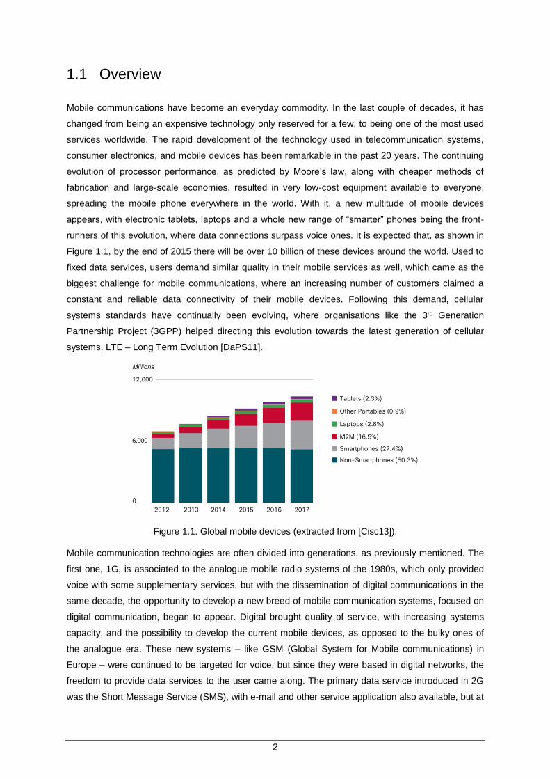
runners of this evolution, where data connections surpass voice ones. It is expected that, as shown in
Figure 1.1, by the end of 2015 there will be over 10 billion of these devices around the world. Used to
fixed data services, users demand similar quality in their mobile services as well, which came as the
biggest challenge for mobile communications, where an increasing number of customers claimed a
constant and reliable data connectivity of their mobile devices. Following this demand, cellular
systems standards have continually been evolving, where organisations like the 3rd Generation
Partnership Project (3GPP) helped directing this evolution towards the latest generation of cellular
systems, LTE – Long Term Evolution [DaPS11].
Figure 1.1. Global mobile devices (extracted from [Cisc13]).
Mobile communication technologies are often divided into generations, as previously mentioned. The
first one, 1G, is associated to the analogue mobile radio systems of the 1980s, which only provided
voice with some supplementary services, but with the dissemination of digital communications in the
same decade, the opportunity to develop a new breed of mobile communication systems, focused on
digital communication, began to appear. Digital brought quality of service, with increasing systems
capacity, and the possibility to develop the current mobile devices, as opposed to the bulky ones of
the analogue era. These new systems – like GSM (Global System for Mobile communications) in
Europe – were continued to be targeted for voice, but since they were based in digital networks, the
freedom to provide data services to the user came along. The primary data service introduced in 2G
was the Short Message Service (SMS), with e-mail and other service application also available, but at

3
a low data rate of 9.6 kbit/s [DaPS11]. Packet data over cellular systems became a reality in the mid-
1990s, with the introduction by 3GPP of General Packet Radio Systems (GPRS) in GSM, and later
near the end of the decade with its Enhancement Data rates for GSM Evolution (EDGE), as illustrated
in Figure 1.2. This technology is common referred to as 2.5G.
Figure 1.2. Evolution of 3GPP mobile communication standards (extracted from [SeTB11]).
The success of these services gave a very clear indication of the potential for applications over packet
data in mobile systems, even with the low data rates practiced at the time and with voice traffic being
clearly dominant. So, consequently, a new generation has emerged, 3G, with a whole new
possibilities for a new range of services. 3GPP defined Universal Mobile Telecommunication Services
(UMTS) in 1999, and it was the European and Japanese standard for 3G, commercially released only
in 2002. But it was only when its add-ons High Speed Downlink Packet Access (HSDPA) and High
Speed Uplink Packet Access (HSUPA) were commercially released in the mid-2000s that data usage
in mobile networks boosted, in many cases exceeding voice traffic volume and becoming the
predominant communication type [SeTB11]. Applications such as audio and video streaming,
interactive gaming, file sharing and applications that require constant synchronism with the Internet,
are invading the market. Hence, data traffic has grown in the last years, with predictions showing that
it will keep on with an exponential grow over the next years, as shown in Figure 1.3.
Figure 1.3. Predicted mobile data traffic (extracted from [Cisc13]).

4
HSPA Evolution (HSPA+) brought faster data rates when it became publicly available in 2008, being
the standard for 3.5G. Approved in 2008 by 3GPP, but released only in late 2009, with first
deployments in Stockholm and Oslo, LTE shattered its predecessors in terms of peak data rate, being
capable of reaching 150 Mbit/s in the downlink. The evolution of data rates provided by 3GPP
standards is pictured in Figure 1.4, being possible to observe that since the development of EDGE
almost 15 years ago, peak data rates has grown more than 600 times.
Figure 1.4. Peak data rate in 3GPP standards (extracted from [HoTo09]).
LTE is often called “4G”, but many also claim that LTE Release 10, also called LTE-Advanced (LTE-
A), is the true evolutionary step, with the LTE Release 8 being labelled as “3.9G”. The specification for
LTE Release 8 formulates an all Internet Protocol (IP) network, with no voice service per se, with
voice calls being performed through Voice over IP (VoIP). Release 9 added minor enhancements to
LTE, namely in the system architecture, but Release 10 brought vast improvements with LTE-A.
Improved spectrum flexibility through Carrier Aggregation (CA) and enhanced downlink Multiple Input
Multiple Output (MIMO), which allows the system to achieve the International Mobile
Telecommunications (IMT) Advanced 4G requirements (such as 1Gbit/s downlink), uplink MIMO,
enhanced Inter-Cell Interference Communication (ICIC), and relaying functionality, where the
possibility of using LTE radio access not only for the network-to-terminal link, but also as a solution for
wireless backhauling, were some of the new upgrades. 3GPP is currently in the concluding stage of
LTE Release 11. In addition to further tuning some of the features of the previous standard, Release
11 includes enhancement support for heterogeneous systems, in other words, the deployment of low-
power network nodes under the coverage of macro-cells [Eric13]. The further evolution of LTE – LTE
Release 12 and beyond – is sometimes referred as LTE-B, as shown in Figure 1.5.
Figure 1.5. Evolution of LTE beyond LTE-A (extracted from [Eric13]).

5
1.2 Motivation and Contents
Since LTE is still being deployed, the traffic load for the network is not very high at the moment. Due
to the low number of current subscribers, performance assessment is not very clear, because many
services are running in very favourable conditions. Sometimes performance can be assessed from
the UMTS network, since both LTE and UMTS have some elements in common. From the user
perspective, it is the end-to-end quality that needs to be classified, or in other terms, the Quality of
Experience (QoE), that involves data rate and delay. On the operator side, other parameters need to
be taken into account, like packet drop and delay variation. Since packet loss can result in highly
noticeable performance issues, while for interactive real-time applications, like VoIP, delay variation
stands out as the main problematic concern, both of these parameters are of the greatest importance
inside the network. Thus, the goal of this work was to model these parameters through statistical
distributions, and to predict their behaviours thought time,
Although one can analyse packet loss and delay variation between two points anywhere inside the
network, it is in the link between the NodeB or eNodeB and the RNC or MME, respectively, that
packet loss and delay variation are most problematic. Due to the capacity issues that sometimes
affect this part of the network, which in a connection between controllers do not occur, the analysis of
both parameters is focused only on these type of links. An identification of the problem source is also
needed, aimed to help the operator tracing to where they are, so that they can take the proper steps
to mitigate them.
In terms of contents, this thesis is divided into five chapters, followed by a set of annexes that add
extra information to the main work done.
In Chapter 2, some fundamental aspects regarding this work are introduced. The basics on how the
systems work are presented, where the network architecture and radio interface of UMTS and LTE,
and how both systems interact with each other, are also shown. A brief analysis is done on the
services and applications both systems are capable of providing, and the various types of parameters
that change accordingly to a specific type of service or application. Also, it is observed how
performance measurements is done, specifically focusing on measurements regarding delay variation
and packet loss. To conclude this chapter, the state of the art of performance measurements and
packet loss and delay variation modelling is presented.
Chapter 3 begins by showing how both parameters are actually calculated. Section 3.2 describes the
statistical distributions that were used to try to model the network sites, and why they were selected,
while Section 3.3 depicts in detail how the goodness-of-fit tests work, and why they are relevant to be
used within the scope of this thesis. Section 3.4 elaborates on the model established to analyse data.
Also in this section, the program developed is detailed and represented with a series of flow charts
that show how its intrinsic mechanics relate to one another, and how the sequential flow of different
analysis steps is processed. Lastly, in Section 3.5, the models for the two types of network links that
connect the sites, microwave and fibre optics, are presented, being accompanied by another group of
diagrams that embrace the basics of the model developed.
6
In Chapter 4, the scenario in which the developed models were applied is presented in the first
section. Both UMTS and LTE network assumptions are made in this section, together with the
definition of parameters to be used within the model. Section 4.2 shows the results of the UMTS
analysis, being divided into three subsections: the first one focus on the results for delay variation, the
second on packet loss, and the third shows an analysis that merges the previous two results into one
single outcome. Section 4.3 shares the same structure of the previous one, but in this case the results
address the LTE network scenario. Section 4.4 contains the theoretical results of the different types of
link model that were used with the scenario provided, and the relationship with the previous delay
variation and packet loss results obtained in the two preceding subsections.
Chapter 5 contains the main conclusions of this thesis, an analysis of the overall obtained results, and
suggestions on future work and different paths that can be taken to improve the analysis done with
this work.
.

7
Chapter 2
Fundamental Concepts and
State of the Art
2 Fundamental Concepts and State of the Art
Chapter 2 gives an overview of the fundamental concepts used in this thesis. Sections 2.1 and 2.2
present the architectural design and radio interfaces of UMTS and LTE, respectively. Section 2.3
elaborates on the services and applications possible within these networks. Section 2.4 gives a
detailed view on how to monitor a network, and the metrics focused on this work, and Section 2.5
concludes the chapter, by providing the state of the art.
8
2.1 UMTS
UMTS principles are presented in this section, where the main contents for both network architecture
and radio interface are based on [HoTo07].
2.1.1 Network Architecture
The UMTS network consists of a number of logical elements. In terms of functionality, two groups
stand out: the Radio Access Network (RAN), which is called UMTS Terrestrial RAN (UTRAN),
handling all the radio-related functions; and the Core Network (CN), which is responsible for switching
and routing calls and data connections to external networks. In order to complete the system, the User
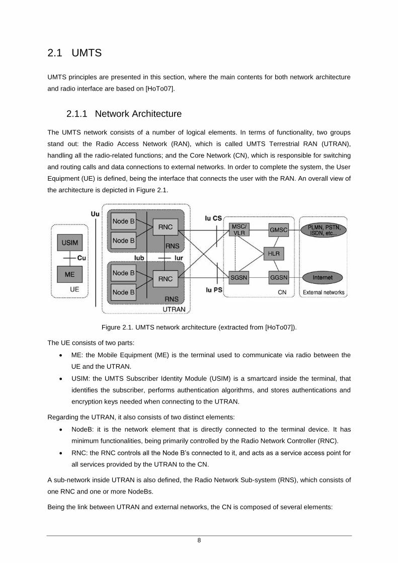
Equipment (UE) is defined, being the interface that connects the user with the RAN. An overall view of
the architecture is depicted in Figure 2.1.
Figure 2.1. UMTS network architecture (extracted from [HoTo07]).
The UE consists of two parts:
ME: the Mobile Equipment (ME) is the terminal used to communicate via radio between the
UE and the UTRAN.
USIM: the UMTS Subscriber Identity Module (USIM) is a smartcard inside the terminal, that
identifies the subscriber, performs authentication algorithms, and stores authentications and
encryption keys needed when connecting to the UTRAN.
Regarding the UTRAN, it also consists of two distinct elements:
NodeB: it is the network element that is directly connected to the terminal device. It has
minimum functionalities, being primarily controlled by the Radio Network Controller (RNC).
RNC: the RNC controls all the Node B’s connected to it, and acts as a service access point for
all services provided by the UTRAN to the CN.
A sub-network inside UTRAN is also defined, the Radio Network Sub-system (RNS), which consists of
one RNC and one or more NodeBs.
Being the link between UTRAN and external networks, the CN is composed of several elements:
9
HLR: the Home Location Register (HLR) is a database where the operator stores the user’s
service profile, e.g., information on allowed services or forbidden roaming areas. When a new
user subscribes to the system, a new entry in the HLR is created, and it remains stored there
as long as the subscription is active.
MSC/VLR: the Mobile Service Switching Centre/Visitor Location Register is the switch (MSC)
and the database (VLR) that serves the UE in its current location for Circuit Switched (CS)
services.
GMSC: the Gateway MSC (GMSC) is the switch where the CN is attached to external CS
networks, with all incoming and outgoing CS connections being handle in this element.
SGSN: the Serving GPRS Support Node (SGSN) functionality is similar of that of MSC/VLR
but for Packet Switch (PS) services instead.
GGSN: the Gateway GPRS Support Node (GGSN) acts similarly to the GMSC but for PS.
Concerning the interfaces linking the elements in the network, UMTS has standards defined as well,
as presented in Figure 2.1. The Cu interface is an electrical interface between the USIM smartcard
and the ME, inside the UE. The radio communication between the UE and the Node B is done through
the Uu interface, while the Iu interface is responsible for connecting the RNC to the CN, for both CS
(RNC to MSC/VLR with IuCS) and PS (RNC to SGSN with IuPS) services. Inside UTRAN, the Iur
interface allows handover between RNCs, while the Iub interface connects the Node Bs to its
responsible RNC.
2.1.2 Radio Interface
UMTS uses Wideband Code Division Multiple Access (WCDMA) as the radio interface, working in the
[1920, 1980] MHz band for Up-Link (UL) and [2110, 2170] MHz for Down-Link (DL). WCDMA is a
wideband Direct-Sequence Code Division Multiple Access (DS-CDMA) system, where user
information bits are spread over a wide bandwidth, by multiplying user data with pre-defined bits called
chips, derived from CDMA spreading codes.
WCDMA uses two types of codes for spreading and multiple access: channelisation codes, where the
signal is spread by extending the occupied bandwidth in accordance to the basic principles of CDMA,
and scrambling codes that help distinguish users and cells. The latter are Orthogonal Variable
Spreading Factor codes, which allow the Spreading Factor to be changed but keeping the
orthogonally between code intact.
With a maximum chip rate of 3.84 Mcps, leading to a carrier bandwidth of 5 MHz, WCDMA supports
highly variable data rates. Each user is allocated with 10 ms frames, during which the user data rate is
kept constant, being able to change only from frame to frame.
The former aspects are common in Releases 99, 5 and 6, although, in order to implement Release 5
and 6, HSDPA and HSUPA respectively, changes were introduced, namely in modulation and SF.
Release 99 uses Quadrature Phase Shift Keying (QPSK) for DL and Binary Phase Shift Keying
(BPSK) for UL, while in HSDPA the modulation is no longer fixed. Adaptive Modulation and Coding
10
(AMC) is used, providing flexibility to match the channel conditions for each user, leading to a constant
transmitted signal power over a frame interval. A summary of the fundamental properties is shown in
Table 2.1.
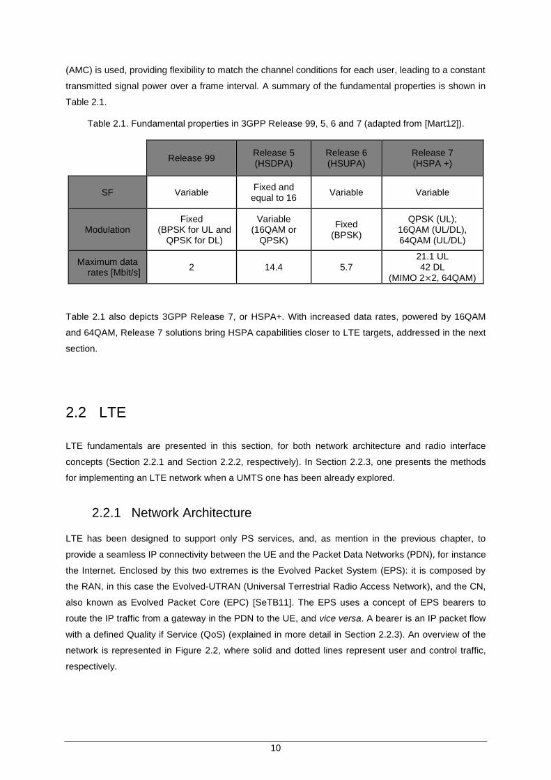
Table 2.1. Fundamental properties in 3GPP Release 99, 5, 6 and 7 (adapted from [Mart12]).
Release 99 Release 5 (HSDPA)
Release 6 (HSUPA)
Release 7 (HSPA +)
SF Variable Fixed and
equal to 16 Variable Variable
Modulation Fixed
(BPSK for UL and QPSK for DL)
Variable (16QAM or
QPSK)
Fixed (BPSK)
QPSK (UL); 16QAM (UL/DL), 64QAM (UL/DL)
Maximum data rates [Mbit/s]
2 14.4 5.7 21.1 UL 42 DL
(MIMO 2×2, 64QAM)
Table 2.1 also depicts 3GPP Release 7, or HSPA+. With increased data rates, powered by 16QAM
and 64QAM, Release 7 solutions bring HSPA capabilities closer to LTE targets, addressed in the next
section.
2.2 LTE
LTE fundamentals are presented in this section, for both network architecture and radio interface
concepts (Section 2.2.1 and Section 2.2.2, respectively). In Section 2.2.3, one presents the methods
for implementing an LTE network when a UMTS one has been already explored.
2.2.1 Network Architecture
LTE has been designed to support only PS services, and, as mention in the previous chapter, to
provide a seamless IP connectivity between the UE and the Packet Data Networks (PDN), for instance
the Internet. Enclosed by this two extremes is the Evolved Packet System (EPS): it is composed by
the RAN, in this case the Evolved-UTRAN (Universal Terrestrial Radio Access Network), and the CN,
also known as Evolved Packet Core (EPC) [SeTB11]. The EPS uses a concept of EPS bearers to
route the IP traffic from a gateway in the PDN to the UE, and vice versa. A bearer is an IP packet flow
with a defined Quality if Service (QoS) (explained in more detail in Section 2.2.3). An overview of the
network is represented in Figure 2.2, where solid and dotted lines represent user and control traffic,
respectively.
11
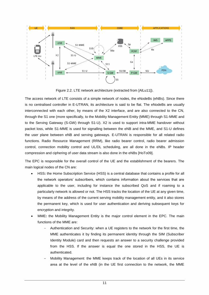
Figure 2.2. LTE network architecture (extracted from [AlLu11]).
The access network of LTE consists of a simple network of nodes, the eNodeBs (eNBs). Since there
is no centralised controller in E-UTRAN, its architecture is said to be flat. The eNodeBs are usually
interconnected with each other, by means of the X2 interface, and are also connected to the CN,
through the S1 one (more specifically, to the Mobility Management Entity (MME) through S1-MME and
to the Serving Gateway (S-GW) through S1-U). X2 is used to support intra-MME handover without
packet loss, while S1-MME is used for signalling between the eNB and the MME, and S1-U defines
the user plane between eNB and serving gateways. E-UTRAN is responsible for all related radio
functions. Radio Resource Management (RRM), like radio bearer control, radio bearer admission
control, connection mobility control and UL/DL scheduling, are all done in the eNBs. IP header
compression and ciphering of user data stream is also done in the eNBs [HoTo09].
The EPC is responsible for the overall control of the UE and the establishment of the bearers. The
main logical nodes of the CN are:
HSS: the Home Subscription Service (HSS) is a central database that contains a profile for all
the network operators’ subscribers, which contains information about the services that are
applicable to the user, including for instance the subscribed QoS and if roaming to a
particularly network is allowed or not. The HSS tracks the location of the UE at any given time,
by means of the address of the current serving mobility management entity, and it also stores
the permanent key, which is used for user authentication and deriving subsequent keys for
encryption and integrity.
MME: the Mobility Management Entity is the major control element in the EPC. The main
functions of the MME are:
- Authentication and Security: when a UE registers to the network for the first time, the
MME authenticates it by finding its permanent identity through the SIM (Subscriber
Identity Module) card and then requests an answer to a security challenge provided
from the HSS. If the answer is equal the one stored in the HSS, the UE is
authenticated.
- Mobility Management: the MME keeps track of the location of all UEs in its service
area at the level of the eNB (in the UE first connection to the network, the MME

12
creates a new entry for the UE and signal the location to the HSS). The MME controls
the setting up and release of resources based on UE’s activity mode changes (active
or idle).
- Managing Subscription Profile and Service Connectivity: when the UE connects to the
network, the MME is responsible for retrieving its subscription profile from the HSS,
and stores this information as long as it is responsible for that UE. The MME will
automatically set up the default bearer, which gives the UE the basic IP connectivity,
and after inspecting the user profile may need to set up more dedicated bearers to
accommodate higher treatment services.
The MME operates exclusively in the CP (Control Plane), processing only signalling
information, and it is not involved in path of UP (User Plane) data, as seen in Figure 2.2.
PCRF: the Policy and Charging Resource Function (PCRF) module is responsible for making
the decisions on how to handle the services in terms of QoS, and provides information to the
Policy Control Enforcement Function (PCEF), that resides in the P-GW, so that appropriate
bearers and policing can be set up.
P-GW: the Packet Data Network Gateway (P-GW) is the element that communicates with the
outside world. It allocates the IP address to the UE, by performing the required DHCP
(Dynamic Host Configuration Protocol) functionality, and filters user IP packets into the
different QoS-based bearers. It also has the functionality for monitoring data traffic flow for
accounting purposes. The P-GW sets up bearers based on request either from the Policy and
Charging Resource Function (PCRF) or the Serving Gateway, which relays information from
the MME.
S-GW: the main function of the Serving Gateway (S-GW) is IP tunnel management and
switching (it acts like a router between eNB and P-GW). It has a minor role in control
functions, as it is only responsible for its own resources and to allocate them based on
requests from the MME, P-GW or the PCRF. During handover between eNBs, the S-GW acts
as the local mobility anchor, as the MME commands the S-GW to switch the bearer from one
eNB to another.
OSS-RC: not showed in Figure 2.2, the Operation Support System for Radio and Core (OSS-
RC) gives a consolidated view of network information (alarms, configurations and performance
indicators). Operators in network management centres use OSS-RC to perform network
management tasks.
The communication between each one of these EPC modules is done through designated interfaces
(all presented in Figure 2.2). The MME uses interface S6a to retrieve subscriber data from the HSS,
S11 to bearer establishment in S-GW, and S10 to support MME changes. S5 is used to establish
bearers between S-GW and P-GW, or between S-GWs, and S8 is analogous to S5 but it is only used
in roaming situations. SGi is the interface in which the UE IP address becomes visible to the PDNs.
Gx is used by PCRF to enforce policy rules to the P-GW, while Rx is used by applications to convey
policy data to the PCRF [AlLu11]. As the same as the OSS-RC, not showing in Figure 2.2 is the Mul
interface, which connects the OSS-RC node to the RAN, carrying operation and maintenance data.
13
2.2.2 Radio Interface
In LTE, the multiple-access technique is based on Orthogonal Frequency Division Multiplexing
(OFDM). ODFM is a special case of multi-carrier transmission, where the large number of narrowband
sub-carriers that compose the main channel are overlapping but orthogonal. The orthogonality
principle provides that at the sampling instant of each individual sub-carrier, the neighbouring sub-
carriers have zero value, avoiding the need to have guard-bands to separate the carriers, therefore
making OFDM highly spectrally efficient [SeTB11]. Although, there is a constant frequency difference
between sub-carriers, which in LTE has been chosen to be 15 kHz, it gives a large enough tolerance
for Doppler shifts due to velocity and for implementation imperfections.
An extension of OFDM is actually used, the Orthogonal Frequency Division Multiple Access (OFDMA),
where different sub-carriers are assigned to different users at the same time, so that each one of them
can be scheduled to receive data simultaneously. OFDMA has been chosen for LTE due to its good
performance in frequency selective fading channels, low complexity of baseband receivers, good
spectral proprieties, handling of multiple bandwidths, frequency domain scheduling, compatibility with
advanced receiver and transmitter technologies, e.g., MIMO [HoTo09], and also because it is suited
for very high data rates and has low sensitivity to fast fading [Corr13].
The DL signal is done through OFDMA. It possesses dimension of time, frequency and svariation,
where the spatial dimension is measured in layers, by means of multiple antenna ports at the eNB.
The time-domain resources for each transmit antenna port are subdivided according to the following
structure: the largest unit of time is the 10 ms radio frame, which is subdivided into ten 1 ms sub-
frames, each of which is split into two 0.5 ms slots. Each slot contains seven OFDM symbols, in case
of the normal cyclic prefix length, or six if the extended cyclic prefix is configured. The cyclic prefix is a
guard period inserted in the beginning of each OFDM symbol, generated by duplicating the last
samples of the symbol and add them to the beginning, designed to avoid Inter-Symbol Interference
(ISI) by ensuring that the delay spread resulted from signal multipath is contained within the cyclic
prefix [SeTB11].
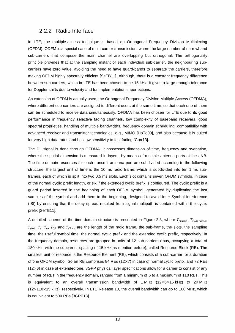
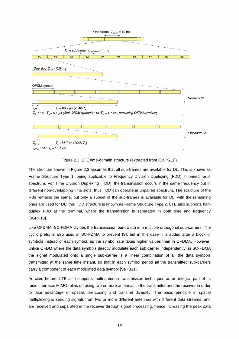
A detailed scheme of the time-domain structure is presented in Figure 2.3, where 𝑇𝑓𝑟𝑎𝑚𝑒 , 𝑇𝑠𝑢𝑏𝑓𝑟𝑎𝑚𝑒,
𝑇𝑠𝑙𝑜𝑡, 𝑇𝑠, 𝑇𝑢, 𝑇𝐶𝑃 and 𝑇𝐶𝑃−𝑒 are the length of the radio frame, the sub-frame, the slots, the sampling
time, the useful symbol time, the normal cyclic prefix and the extended cyclic prefix, respectively. In
the frequency domain, resources are grouped in units of 12 sub-carriers (thus, occupying a total of
180 kHz, with the subcarrier spacing of 15 kHz as mention before), called Resource Block (RB). The
smallest unit of resource is the Resource Element (RE), which consists of a sub-carrier for a duration
of one OFDM symbol. So an RB comprises 84 REs (12×7) in case of normal cyclic prefix, and 72 REs
(12×6) in case of extended one. 3GPP physical layer specifications allow for a carrier to consist of any
number of RBs in the frequency domain, ranging from a minimum of 6 to a maximum of 110 RBs. This
is equivalent to an overall transmission bandwidth of 1 MHz (12×6×15 kHz) to 20 MHz
(12×110×15 kHz), respectively. In LTE Release 10, the overall bandwidth can go to 100 MHz, which
is equivalent to 500 RBs [3GPP13].
14
Figure 2.3. LTE time-domain structure (extracted from [DaPS11]).
The structure shown in Figure 2.3 assumes that all sub-frames are available for DL. This is known as
Frame Structure Type 1, being applicable to Frequency Division Duplexing (FDD) in paired radio
spectrum. For Time Division Duplexing (TDD), the transmission occurs in the same frequency but in
different non-overlapping time slots, thus TDD can operate in unpaired spectrum. The structure of the
RBs remains the same, but only a subset of the sub-frames is available for DL, with the remaining
ones are used for UL; this TDD structure is known as Frame Structure Type 2. LTE also supports half-
duplex FDD at the terminal, where the transmission is separated in both time and frequency
[3GPP13].
Like OFDMA, SC-FDMA divides the transmission bandwidth into multiple orthogonal sub-carriers. The
cyclic prefix is also used in SC-FDMA to prevent ISI, but in this case it is added after a block of
symbols instead of each symbol, as the symbol rate takes higher values than in OFDMA. However,
unlike OFDM where the data symbols directly modulate each sub-carrier independently, in SC-FDMA
the signal modulated onto a single sub-carrier is a linear combination of all the data symbols
transmitted at the same time instant, so that in each symbol period all the transmitted sub-carriers
carry a component of each modulated data symbol [SeTB11].
As cited before, LTE also supports multi-antenna transmission techniques as an integral part of its
radio interface. MIMO relies on using two or more antennas in the transmitter and the receiver in order
to take advantage of spatial, pre-coding and transmit diversity. The basic principle in spatial
multiplexing is sending signals from two or more different antennas with different data streams, and
are received and separated in the receiver through signal processing, hence increasing the peak data

15
rates by a factor of two or more, depending on the configuration of the antennas. In pre-coding,
signals transmitted from the different antennas are weighted with the objective of maximising the
Signal-to-Noise Ratio (SNR). Finally, transmit diversity relies on sending the same signal from multiple
antennas with some code to exploit the gains from independent fading between antennas [HoTo09].
In terms of spectrum, 3GPP has specified 29 FDD and 12 TDD operating bands for the radio access
in LTE [3GPP13c], which covers the main frequency bands from 700 MHz to 900 MHz, 1500 MHz to
2100 MHz, and also the 2500 MHz, 2600 MHz, 3500 MHz and 3600 MHz bands. In Portugal, the
bands chosen by the Portuguese Telecommunication Authority ANACOM for the three main
Portuguese operators (VODAFONE, PT and NOS) were the 800 MHz, 1800 MHz and 2600 MHz
bands [ANAC11].
2.2.3 Coexistence with UMTS
The content of this subsection is based on [4GAm11] and [Moto09].
Being two fundamentally different systems, migrating from UMTS to LTE involves a major change in
networking technologies, moving from a CS network to an all-IP technology. As with any technology
evolution, the question is how to address the impact of new network elements, defined for LTE, on the
legacy network.
In case the 3G RNC and SGSN are not being upgraded, connection with the new LTE elements is
done using the existing interfaces and mobility mechanisms. The GTP based Gn interface used to
connect the SGSN to the GGSN and also other SGSN, is also used to communicate with the EPC
elements, connecting the SGSN to the MME and P-GW. With this, the SGSN sees the new EPC
nodes as simply other UMTS elements. Hence, all adaptations are made in the LTE/EPC side alone,
where the MME and the P-GW both support the Gn interface towards the SGSN.
Sessions from an LTE capable UE are always anchored on the P-GW. Inter-access sessions mobility
is possible when the UE moves between the UTRAN and E-UTRAN coverage area with the help of
the Gn interface between the SGSN and the MME and the PG-W. In terms of subscribers’ database,
both HLR and HSS are combined together, so both SGSN and MME have access to it.
The benefit with this implementation is that no upgrades are required in the existing networks, and it is
viable until the operator decides to upgrade to S3/S4 network interfaces. A schematic of this type of
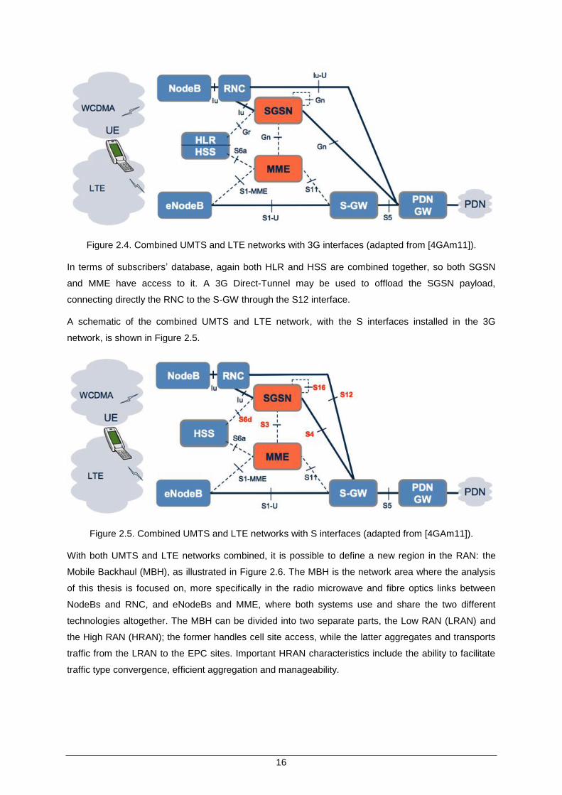
combined UMTS and LTE networks is shown in Figure 2.4.
In the case that the SGSN has been upgraded to support LTE defined “S” interfaces, S3, S4, and S12,
one could use the S-GW as the common anchor for all the 3GPP access technologies, leading to a
simplified network architecture. Inter-access session mobility is possible when the UE moves between
the UTRAN and E-UTRAN coverage area by the S3 interface, connecting the SGSN to the MME, and
the S4 interface, connecting the SGSN to the S-GW.
16
Figure 2.4. Combined UMTS and LTE networks with 3G interfaces (adapted from [4GAm11]).
In terms of subscribers’ database, again both HLR and HSS are combined together, so both SGSN
and MME have access to it. A 3G Direct-Tunnel may be used to offload the SGSN payload,
connecting directly the RNC to the S-GW through the S12 interface.
A schematic of the combined UMTS and LTE network, with the S interfaces installed in the 3G
network, is shown in Figure 2.5.
Figure 2.5. Combined UMTS and LTE networks with S interfaces (adapted from [4GAm11]).
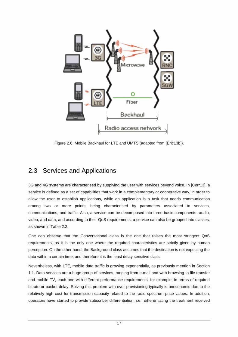
With both UMTS and LTE networks combined, it is possible to define a new region in the RAN: the
Mobile Backhaul (MBH), as illustrated in Figure 2.6. The MBH is the network area where the analysis
of this thesis is focused on, more specifically in the radio microwave and fibre optics links between
NodeBs and RNC, and eNodeBs and MME, where both systems use and share the two different
technologies altogether. The MBH can be divided into two separate parts, the Low RAN (LRAN) and
the High RAN (HRAN); the former handles cell site access, while the latter aggregates and transports
traffic from the LRAN to the EPC sites. Important HRAN characteristics include the ability to facilitate
traffic type convergence, efficient aggregation and manageability.
17
Figure 2.6. Mobile Backhaul for LTE and UMTS (adapted from [Eric13b]).
2.3 Services and Applications
3G and 4G systems are characterised by supplying the user with services beyond voice. In [Corr13], a
service is defined as a set of capabilities that work in a complementary or cooperative way, in order to
allow the user to establish applications, while an application is a task that needs communication
among two or more points, being characterised by parameters associated to services,
communications, and traffic. Also, a service can be decomposed into three basic components: audio,
video, and data, and according to their QoS requirements, a service can also be grouped into classes,
as shown in Table 2.2.
One can observe that the Conversational class is the one that raises the most stringent QoS
requirements, as it is the only one where the required characteristics are strictly given by human
perception. On the other hand, the Background class assumes that the destination is not expecting the
data within a certain time, and therefore it is the least delay sensitive class.
Nevertheless, with LTE, mobile data traffic is growing exponentially, as previously mention in Section
1.1. Data services are a huge group of services, ranging from e-mail and web browsing to file transfer
and mobile TV, each one with different performance requirements, for example, in terms of required
bitrate or packet delay. Solving this problem with over-provisioning typically is uneconomic due to the
relatively high cost for transmission capacity related to the radio spectrum price values. In addition,
operators have started to provide subscriber differentiation, i.e., differentiating the treatment received

18
by different subscriber groups for the same service. These groups can be defined in any way suitable
to the operator, like corporate versus private subscribers, or privilege groups, e.g., police or fire-
fighters.
Table 2.2. Service classes and requirements for UMTS QoS (extracted from [Corr13]).
Service Class Conversational Streaming Interactive Background
Real Time Yes Yes No No
Symmetric Yes No No No
Switching CS CS PS PS
Guaranteed Bit
Rate Yes Yes No No
Affordable
Delay Minimum (Fixed)
Minimum
(Variable)
Moderate
(Variable) High (Variable)
Buffer No Yes Yes Yes
Bursty No No Yes Yes
Example Voice Video-clip WWW E-mail
There is a need to standardise simple and effective QoS mechanisms that allow the operator to
enable service and subscriber differentiation and to control the performance experienced by the
packet traffic of a certain service and subscriber group. In order to solve this problem, 3GPP specified
for the EPS the concept of EPS bearer. A bearer uniquely identifies packet flows that receive common
QoS treatment, providing different management for traffic with different QoS requirements, by
associating them a packet flow defined by a five-tuple-based packet filter (source and destination IP
address, source and destination port number, and protocol ID). Broadly, bearers can be classified into
two main categories based on the QoS they provide:
Minimum Guaranteed Bit Rate (GBR) bearers: these have associated GBR value for which
dedicated transmission resources are permanently allocated. Bit rates higher than the GBR
may be offered if the resources are available at the time. In those cases, a Maximum Bit Rate
(MBR) parameter sets up an upper limit to the bit rate value the bearer can accommodate.
Non-GBR bearers: non-GRB bearers do not guarantee any specific bit rate, and no bandwidth
resources are permanently allocated to it.
Also, each bearer has an associated QoS Class Identifier (QCI) and an Allocation and Retention
Priority (ARP). The QCI is an index number that identifies a set of pre-defined parameter values for
four QoS attributes (resource type, priority, delay and loss rate) while ARP indicates the priority of the
bearer compared to other bearers, aiding in the decision of which bearer to drop in case of congestion
situation. Nine QCI classes have been standardised, as seen in Table 2.3. The parameters of these
QCI classes are:
Resource type: indicates which classes will have GBR associated to them;
Priority: defines the priority for the packet scheduling of the radio interface;

19
Delay Budget: helps the packet scheduler to maintain sufficient scheduling rate to meet the
delay requirements for the bearer;
Loss Rate: helps to use appropriate Radio Link Control (RLC) settings, i.e., number of re-
transmissions.
Table 2.3. Standardised QoS Class Identifiers (extracted from [3GPP13b]).
QCI Resource
Type Priority
Packet Delay
Budget [ms]
Packet Error
Loss Rate Example Services
1
GBR
2 100 10−2 Conversational voice
2 4 150 10−3 Conversational voice (live streaming)
3 3 50 10−3 Real-time gaming
4 5 300 10−6 Non-conversational video (buffered
streaming)
5
Non-GBR
1 100 10−6 IMS signalling
6 6 300 10−6 Video (buffered streaming), TCP-
based (e.g. www, e-mail, chat, FTP)
7 7 100 10−3 Voice, video (live streaming),
interactive gaming
8 8 300 10−6
Video (buffered streaming), TCP-
based (e.g. www, e-mail, chat, FTP) 9 9
In addition, operators can create new classes, besides the ones presented, to implement inside their
own network if they seem necessary.
2.4 Performance Monitoring
The content of this section is based on [ESAT], [ITUT08] and [Eric13d]. A brief description on
performance monitoring relationships is given, as well as a typical process on how to measure the
parameters focused on this work.
Monitoring and statistical measures is a very important part of the Operation and Maintenance (OAM)
of a network. The radio network statistic and recording functions can be used for monitoring and
optimisation of the radio network performance, evaluation and optimisation of the radio network
features, dimensioning of the radio network, and troubleshooting.
Nonetheless this procedures being valid, the OAM solution enhances network management
capabilities, supporting the main requirements for good backhaul performance. Regardless of the
specific service in question, OAM adds monitoring in terms of the performance management of the

20
integrity, accessibility and retainability of such services. The OAM solution for mobile backhaul
consists of several entities, such as Ethernet OAM and IP OAM. Ethernet OAM provides remote
monitoring of Ethernet networks, delivering two major features for Ethernet services: Connectivity
Fault Management and Performance Management.
This section provides a description of the two main types of Ethernet OAM: Link OAM and Service
OAM). Link OAM is limited to a physical link and Service OAM is for a service purpose. There are no
dependencies between the two, either one or both OAM types may be used within the same Ethernet
network.
Link OAM, based on IEEE 802.3ah protocol [Eric13d], is a slow protocol, in contrast to Service OAM,
with frames being exchanged at a rate no faster than 10 per second. Link OAM is especially suited for
edge devices with limited computational resources, supporting features such as discovering remote
devices, querying the configurations of remote devices and reporting link statistics.
On the other hand, Service OAM means end-to-end management of Ethernet services. Two main
standard exist: ITU-T Y.1731 and IEEE 802.1ag [Eric13d]. Both define an OAM framework for
Ethernet based networks and define OAM function for fault management and performance monitoring.
The concepts and entities of Service OAM, defined by the protocols, are:
ME: The Maintenance Entity represents an entity that requires management and is a
relationship between two maintenance entity group end points (MEP).
MEG: An ME Group includes different MEs that exists in the same administrative boundary or
have the same MD Level.
MEP: An MEG End Point marks the end point of a MEG, which is capable of initiating and
terminating OAM frames for performance monitoring. These are distinct from the transit
Ethernet flows, but always follow the path of the data streams that they relate.
DOWN MEP: An MEP operating on and in the direction out from an interface.
UP MEP: An MEP operating on an interface in the direction toward the internal bridge
component.
MD Level: a Maintenance Domain Level manages a collection of Maintenance Associations
(MA) for which faults in connectivity are managed and end-to-end performances can also be
measured.
MIP: a Maintenance Intermediate Point is an intermediate point in an MEG. It is capable of
reacting to some on-demand OAM frames, allowing more precise diagnosis of connectivity
failure locations.
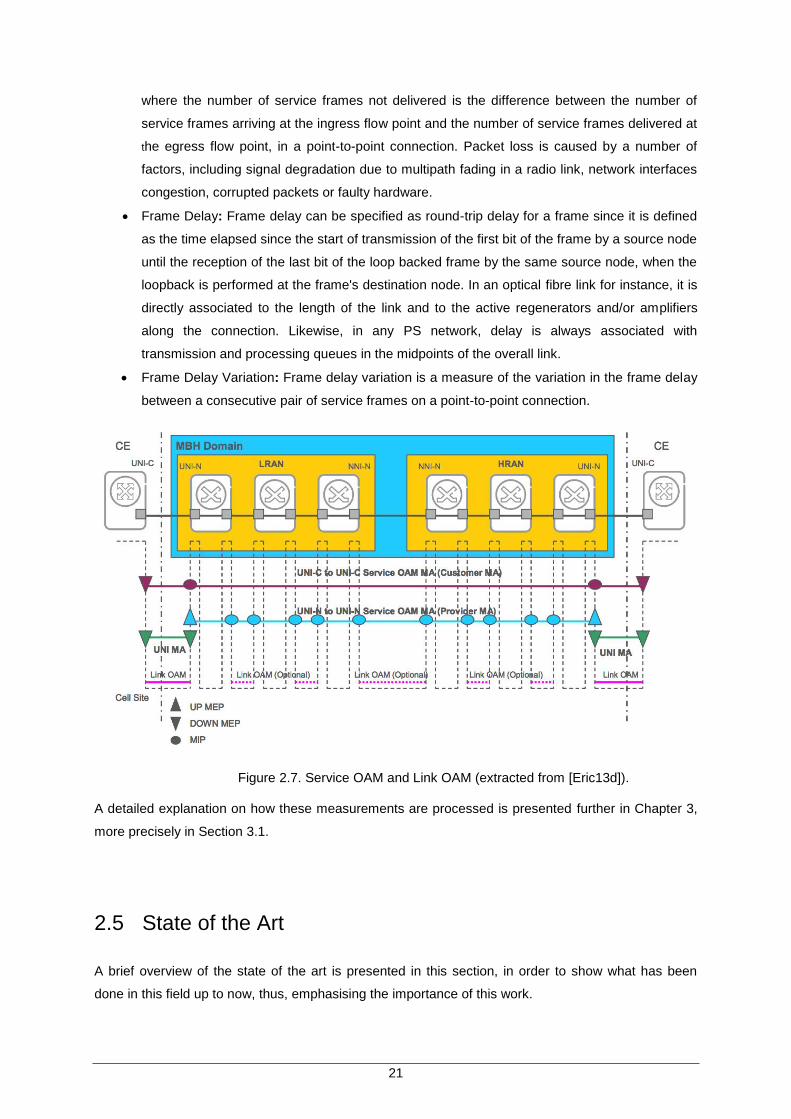
A comparison between Service OAM and Link OAM, as well as the entities of Service OAM, is
illustrated in Figure 2.7.
As said before, OAM functions for performance monitoring allow measurements of different
performance parameters. This thesis focuses on:
Frame Loss Ratio: Frame loss ratio is defined as a ratio between the number of service
frames not delivered divided by the total number of service frames during a time interval,
21
where the number of service frames not delivered is the difference between the number of
service frames arriving at the ingress flow point and the number of service frames delivered at
the egress flow point, in a point-to-point connection. Packet loss is caused by a number of
factors, including signal degradation due to multipath fading in a radio link, network interfaces
congestion, corrupted packets or faulty hardware.
Frame Delay: Frame delay can be specified as round-trip delay for a frame since it is defined
as the time elapsed since the start of transmission of the first bit of the frame by a source node
until the reception of the last bit of the loop backed frame by the same source node, when the
loopback is performed at the frame's destination node. In an optical fibre link for instance, it is
directly associated to the length of the link and to the active regenerators and/or amplifiers
along the connection. Likewise, in any PS network, delay is always associated with
transmission and processing queues in the midpoints of the overall link.
Frame Delay Variation: Frame delay variation is a measure of the variation in the frame delay
between a consecutive pair of service frames on a point-to-point connection.
Figure 2.7. Service OAM and Link OAM (extracted from [Eric13d]).
A detailed explanation on how these measurements are processed is presented further in Chapter 3,
more precisely in Section 3.1.
2.5 State of the Art
A brief overview of the state of the art is presented in this section, in order to show what has been
done in this field up to now, thus, emphasising the importance of this work.
22
Regarding the frame delay measurement, in [LSRM12] a comparison between one-way delays in
HSPA and LTE networks is made, adopting a measurement methodology that is a hybrid between
active probing and passive monitoring. Probe packets are injected into the network and captured at an
intermediate interface at the edges of the CN. In this way, besides comparing one-way delays
separately for the UL and DL directions, there is also the possibility to split the total delay into its RAN
and CN components. Ensuring a fair comparison between both networks, by transmitting packets
following the same sending patterns with the same modem connected to base stations located at the
same site, and synchronising all the devices involved, the authors found that, for DL, LTE displays
roughly half of the one-way delay compared to HSPA. For the UL, the one-way delay of HSPA
depends strongly on the data rate and packet size, where at low rates with large packet sizes the UL
delay of HSPA is higher than LTE, while for all other settings it is sensibly lower. Lastly, considering a
fixed average data rate, the authors found that the LTE latency is insensitive to packet size. Instead,
for HSPA there is a strong positive correlation between packet size and one-way delay.
In [PHJI07], the authors use the QoSMeT tool and measure application performance over 3G
networks, focusing mainly on delay behaviour, which is critical for conversational applications like
VoIP. QoSMeT is a passive QoS measurement tool, capable of monitoring QoS performance and
enables end-to-end real-time quality measurements of any networking applications in both
communicating directions, and it is based on data link level measurements, i.e., it sniffs both the
departing and arriving packets directly from the network interface device. In this way, QoSMeT records
essential packet information, including accurate arrival and departure times of the packets (time
stamps). For packet loss, QoSMeT calculates it by considering lost each packet that does not get an
acknowledgement (corresponding arrival timestamp) by the control packet from the peer node.
Regarding the delay, QoSMeT measures the total end-to-end delay experienced by individual packets,
thus including all the possible delay components (e.g., propagation, queuing, and transmission
delays), where clock synchronisation problems are overcome through authors own GPS drivers.
In [ArFi10], the authors elaborate on the influence of packet size on the one-way delay, using an
entirely passive measurement technique that will not affect any part of the network. In this case, the
synchronisation problem is overcome using NTP. The authors conclude, as previously stated, that the
packet size has pronounced influence on the one-way delay.
Considering a manufacturer approach, Ericsson has the IP Probe System [Eric12], which is an active
QoS and performance-monitoring system based on distributed measurement probes, with centralised
configuration, management and reporting. The system is intended for both 24/7 network supervision or
fault localisation activities, utilising both fixed installation and light-weight portable probes. The active
probes are populated into the network, where the measurements should be carried out, generating
and sending small traffic streams through the network that can be monitored afterwards. Although
being based on the Y.1731 protocol, it has the downside of requiring extra hardware to be
implemented in the network.
One last note on the state of the art of this work is that, usually, this type of information, regarding
performance measurements and monitoring, is confidential and restricted to mobile operators. So the

23
available information is scarce, since it is comprehensible that companies do not put publicly available
information that might be used by competitor entities to improve their performance monitoring
solutions.

24

25
Chapter 3
Performance Analysis Model
3 Performance Analysis Model
In Chapter 3, one can find all the information regarding the developed model. Section 3.1 presents the
parameters to be evaluated, Section 3.2 describes the distributions used to model the parameters,
while on Section 3.3 the test used to verify the quality of the model fitted is shown. The information
regarding the performance analysis program is in Section 3.4, and in Section 3.5 the model for the
network link is presented.
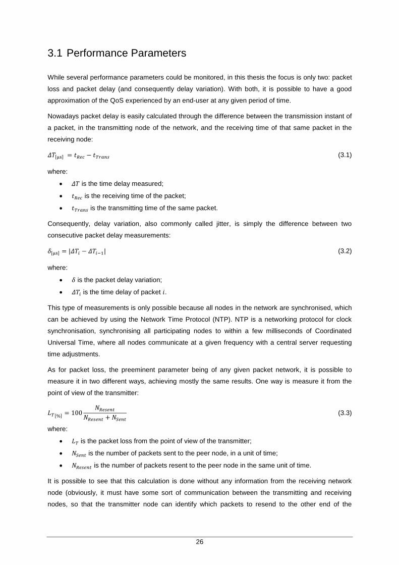
26
3.1 Performance Parameters
While several performance parameters could be monitored, in this thesis the focus is only two: packet
loss and packet delay (and consequently delay variation). With both, it is possible to have a good
approximation of the QoS experienced by an end-user at any given period of time.
Nowadays packet delay is easily calculated through the difference between the transmission instant of
a packet, in the transmitting node of the network, and the receiving time of that same packet in the
receiving node:
𝛥𝑇[μs] = 𝑡𝑅𝑒𝑐 − 𝑡𝑇𝑟𝑎𝑛𝑠 (3.1)
where:
𝛥𝑇 is the time delay measured;
𝑡𝑅𝑒𝑐 is the receiving time of the packet;
𝑡𝑇𝑟𝑎𝑛𝑠 is the transmitting time of the same packet.
Consequently, delay variation, also commonly called jitter, is simply the difference between two
consecutive packet delay measurements:
𝛿[μs] = |𝛥𝑇𝑖 − 𝛥𝑇𝑖−1| (3.2)
where:
𝛿 is the packet delay variation;
𝛥𝑇𝑖 is the time delay of packet 𝑖.
This type of measurements is only possible because all nodes in the network are synchronised, which
can be achieved by using the Network Time Protocol (NTP). NTP is a networking protocol for clock
synchronisation, synchronising all participating nodes to within a few milliseconds of Coordinated
Universal Time, where all nodes communicate at a given frequency with a central server requesting
time adjustments.
As for packet loss, the preeminent parameter being of any given packet network, it is possible to
measure it in two different ways, achieving mostly the same results. One way is measure it from the
point of view of the transmitter:
𝐿𝑇[%] = 100𝑁𝑅𝑒𝑠𝑒𝑛𝑡
𝑁𝑅𝑒𝑠𝑒𝑛𝑡 + 𝑁𝑆𝑒𝑛𝑡 (3.3)
where:
𝐿𝑇 is the packet loss from the point of view of the transmitter;
𝑁𝑆𝑒𝑛𝑡 is the number of packets sent to the peer node, in a unit of time;
𝑁𝑅𝑒𝑠𝑒𝑛𝑡 is the number of packets resent to the peer node in the same unit of time.
It is possible to see that this calculation is done without any information from the receiving network
node (obviously, it must have some sort of communication between the transmitting and receiving
nodes, so that the transmitter node can identify which packets to resend to the other end of the

27
network link, but that is not taken into account here).
The other way of measuring packet loss is through the perspective of the receiver network node,
which is calculated from:
𝐿𝑅[%] = 100𝑁𝐿
𝑁𝐿 +𝑁𝑅 (3.4)
where:
𝐿𝑅 is the packet loss from the point of view of the receiver;
𝑁𝑅 is the number of packets received by the node, in a unit of time;
𝑁𝐿 is the number of packets that were not correctly received by the node, or lost, in the same
unit of time, due to, e.g., wrong decoding, wrong header, wrong payload, or destroyed frames.
Likewise, the calculation is done without the packet transmitter intervention, just by the
acknowledgement by the receiver of the improper packets received.
It can be seen that the results obtained from 𝐿𝑇 and 𝐿𝑅 are intrinsically connected through the values
of 𝑁𝑅𝑒𝑠𝑒𝑛𝑡 and 𝑁𝐿, since the number of packets that are in need to be resented by the transmitter end
is equal to the number of packets that are in short, due to some sort of problem, in the receiver part of
the connection.
3.2 Statistical Distributions
In order to evaluate the performance of a site, one has to analyse the data originated from it. On the
other hand, if a prediction has to be made, based on the collected and analysed data, on whether the
same site will have performance problems in the future, regarding delay variation or packet loss, a
statistical model has to be developed to estimate the evolution of the concerned performance
parameters associated to the base station. One can accomplish this by finding the best statistical
distribution that fits the evaluated data, sharing its properties in terms of behaviour over time, average
value and standard deviation, which are all characteristic, and sometimes similar, for each distribution.
Of all the statistical distributions available, a small group was taken into account upon the
development of the model that is used in this thesis. The considered distributions were the following:
Gamma distribution;
Generalised Extreme Value distribution;
Inverse Gaussian distribution;
Logistic distribution;
Log-logistic distribution;
Log-normal distribution;
Nakagami distribution;
Rayleigh distribution;
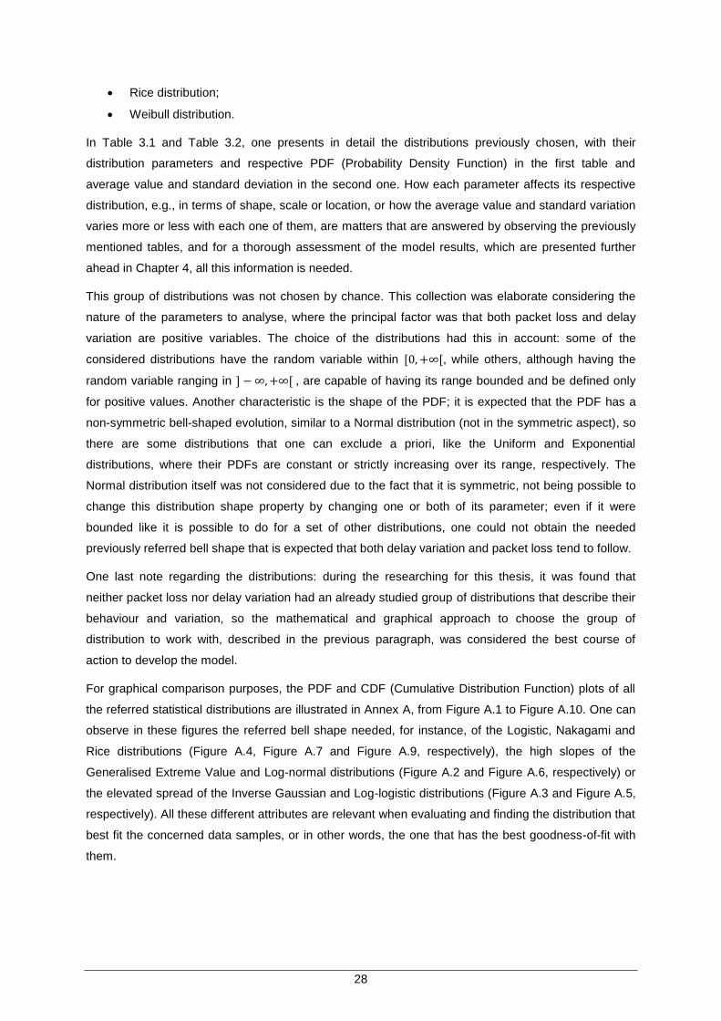
28
Rice distribution;
Weibull distribution.
In Table 3.1 and Table 3.2, one presents in detail the distributions previously chosen, with their
distribution parameters and respective PDF (Probability Density Function) in the first table and
average value and standard deviation in the second one. How each parameter affects its respective
distribution, e.g., in terms of shape, scale or location, or how the average value and standard variation
varies more or less with each one of them, are matters that are answered by observing the previously
mentioned tables, and for a thorough assessment of the model results, which are presented further
ahead in Chapter 4, all this information is needed.
This group of distributions was not chosen by chance. This collection was elaborate considering the
nature of the parameters to analyse, where the principal factor was that both packet loss and delay
variation are positive variables. The choice of the distributions had this in account: some of the
considered distributions have the random variable within [0, +∞[, while others, although having the
random variable ranging in ] − ∞,+∞[ , are capable of having its range bounded and be defined only
for positive values. Another characteristic is the shape of the PDF; it is expected that the PDF has a
non-symmetric bell-shaped evolution, similar to a Normal distribution (not in the symmetric aspect), so
there are some distributions that one can exclude a priori, like the Uniform and Exponential
distributions, where their PDFs are constant or strictly increasing over its range, respectively. The
Normal distribution itself was not considered due to the fact that it is symmetric, not being possible to
change this distribution shape property by changing one or both of its parameter; even if it were
bounded like it is possible to do for a set of other distributions, one could not obtain the needed
previously referred bell shape that is expected that both delay variation and packet loss tend to follow.
One last note regarding the distributions: during the researching for this thesis, it was found that
neither packet loss nor delay variation had an already studied group of distributions that describe their
behaviour and variation, so the mathematical and graphical approach to choose the group of
distribution to work with, described in the previous paragraph, was considered the best course of
action to develop the model.
For graphical comparison purposes, the PDF and CDF (Cumulative Distribution Function) plots of all
the referred statistical distributions are illustrated in Annex A, from Figure A.1 to Figure A.10. One can
observe in these figures the referred bell shape needed, for instance, of the Logistic, Nakagami and
Rice distributions (Figure A.4, Figure A.7 and Figure A.9, respectively), the high slopes of the
Generalised Extreme Value and Log-normal distributions (Figure A.2 and Figure A.6, respectively) or
the elevated spread of the Inverse Gaussian and Log-logistic distributions (Figure A.3 and Figure A.5,
respectively). All these different attributes are relevant when evaluating and finding the distribution that
best fit the concerned data samples, or in other words, the one that has the best goodness-of-fit with
them.
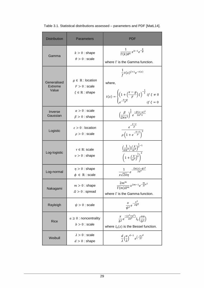
29
Table 3.1. Statistical distributions assessed – parameters and PDF [MatL14].
Distribution Parameters PDF
Gamma 𝑘 > 0 : shape
𝜃 > 0 : scale
1
Γ(𝑘)𝜃𝑘𝑥𝑘−1𝑒−
𝑘𝜃
where Γ is the Gamma function.
Generalised Extreme
Value
𝑔 ∈ ℝ : location
𝐹 > 0 : scale
𝜉 ∈ ℝ : shape
1
𝑓𝑡(𝑥)𝜉+1𝑒−𝑡(𝑥)
where,
𝑡(𝑥) = {(1 + (
𝑥 − 𝑔
𝐹) 𝜉)
−1𝜉 𝑖𝑓 𝜉 ≠ 0
𝑒−𝑥−𝑔𝐹 𝑖𝑓 𝜉 = 0
Inverse Gaussian
𝛼 > 0 : scale
𝛽 > 0 : shape (𝛽
2𝜋𝑥3)
12
𝑒−𝛽(𝑥−𝛼)2
2𝛼2𝑥
Logistic 휀 > 0 : location
𝜌 > 0 : scale
𝑒−𝑥−𝜀𝜌
𝜌 (1 + 𝑒−𝑥−𝜀𝜌 )
2
Log-logistic 𝜏 ∈ ℝ: scale
𝜐 > 0 : shape
(1𝜐𝑒𝜏
) (𝑥𝑒𝜏)
1𝜐−1
(1 + (𝑥𝑒𝜏)
1𝜐)
2
Log-normal 𝜂 > 0 : shape
𝜙 ∈ ℝ : scale
1
𝑥√2𝜋𝜂𝑒−(ln(𝑥)−𝜙)2
2𝜂2
Nakagami 𝑚 > 0 : shape
𝛺 > 0 : spread
2𝑚𝑚
Γ(𝑚)𝛺𝑚𝑥2𝑚−1𝑒−
𝑚𝛺𝑥2
where Γ is the Gamma function.
Rayleigh 𝜓 > 0 : scale 𝑥
𝜓2𝑒−𝑥2
2𝜓2
Rice 𝑎 ≥ 0 : noncentrality
𝑏 > 0 : scale
𝑥
𝑏2𝑒−(𝑥2+𝑎2)
2𝑏2 𝐼0 (𝑥𝑎
𝑏2)
where 𝐼0(𝑧) is the Bessel function.
Weibull 𝜆 > 0 : scale
𝑑 > 0 : shape
𝑑
𝜆(𝑥
𝜆)𝑑−1
𝑒(−𝑥𝜆)𝑑
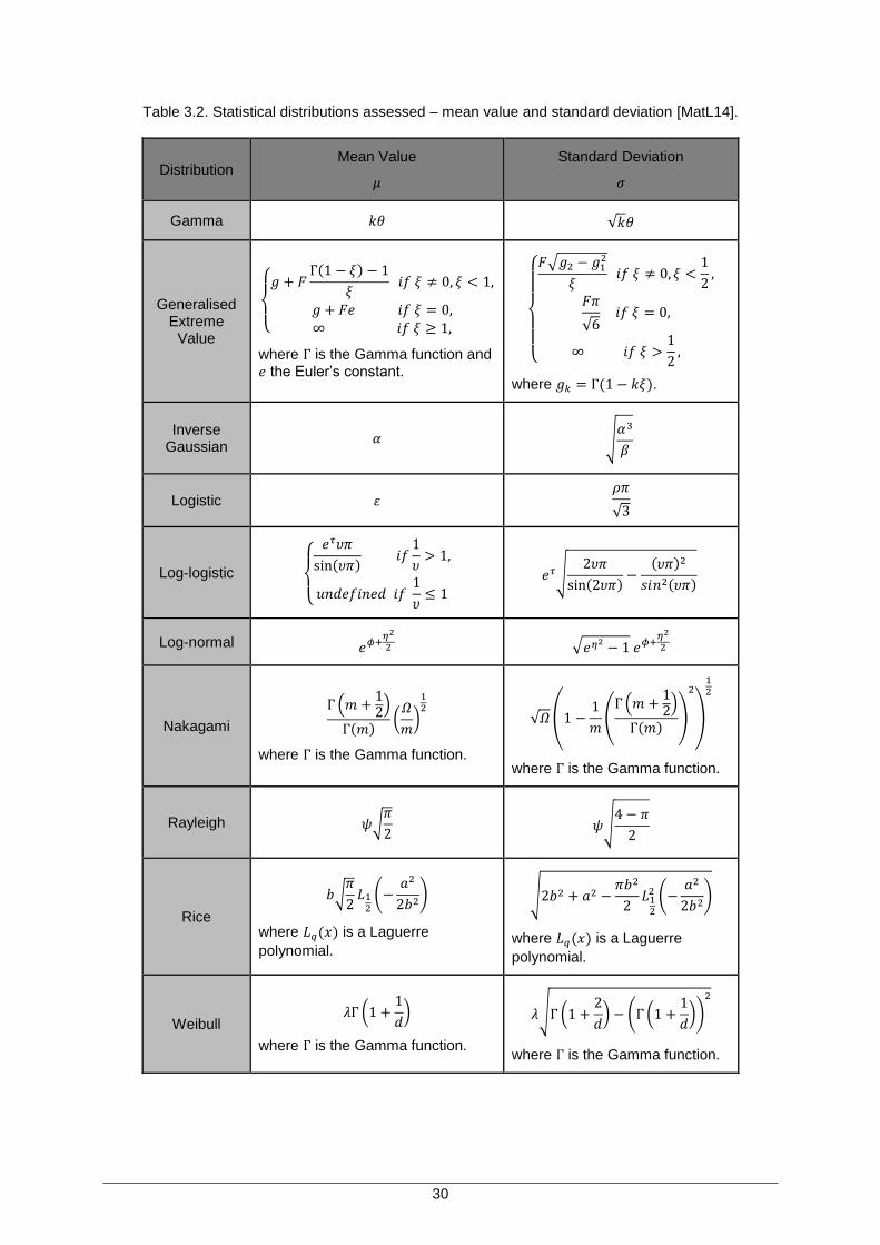
30
Table 3.2. Statistical distributions assessed – mean value and standard deviation [MatL14].
Distribution Mean Value
𝜇
Standard Deviation
𝜎
Gamma 𝑘𝜃 √𝑘𝜃
Generalised Extreme
Value {
𝑔 + 𝐹Γ(1 − 𝜉) − 1
𝜉 𝑖𝑓 𝜉 ≠ 0, 𝜉 < 1,
𝑔 + 𝐹𝑒 𝑖𝑓 𝜉 = 0,∞ 𝑖𝑓 𝜉 ≥ 1,
where Γ is the Gamma function and 𝑒 the Euler’s constant.
{
𝐹√𝑔2 − 𝑔1
2
𝜉 𝑖𝑓 𝜉 ≠ 0, 𝜉 <
1
2,
𝐹𝜋
√6 𝑖𝑓 𝜉 = 0,
∞ 𝑖𝑓 𝜉 >1
2,
where 𝑔𝑘 = Γ(1 − 𝑘𝜉).
Inverse Gaussian
𝛼 √𝛼3
𝛽
Logistic 휀 𝜌𝜋
√3
Log-logistic
{
𝑒𝜏𝜐𝜋
sin(𝜐𝜋) 𝑖𝑓
1
𝜐> 1,
𝑢𝑛𝑑𝑒𝑓𝑖𝑛𝑒𝑑 𝑖𝑓 1
𝜐≤ 1
𝑒𝜏√2𝜐𝜋
sin(2𝜐𝜋)−
(𝜐𝜋)2
𝑠𝑖𝑛2(𝜐𝜋)
Log-normal 𝑒𝜙+𝜂2
2 √𝑒𝜂2− 1 𝑒𝜙+
𝜂2
2
Nakagami
Γ (𝑚 +12)
Γ(𝑚)(𝛺
𝑚)
12
where Γ is the Gamma function.
√𝛺(1 −1
𝑚(Γ(𝑚 +
12)
Γ(𝑚))
2
)
12
where Γ is the Gamma function.
Rayleigh 𝜓√𝜋
2 𝜓√
4 − 𝜋
2
Rice
𝑏√𝜋
2𝐿12(−
𝑎2
2𝑏2)
where 𝐿𝑞(𝑥) is a Laguerre
polynomial.
√2𝑏2 + 𝑎2 −𝜋𝑏2
2𝐿12
2 (−𝑎2
2𝑏2)
where 𝐿𝑞(𝑥) is a Laguerre
polynomial.
Weibull 𝜆Γ (1 +
1
𝑑)
where Γ is the Gamma function.
𝜆√Γ (1 +2
𝑑) − (Γ (1 +
1
𝑑))
2
where Γ is the Gamma function.
31
3.3 Goodness-of-fit
The basis for the content of this subsection was taken from [RomJ04].
When assuming that data follows a specific distribution, if the assumed distribution does not hold then
the confidence levels of the hypothesis tests implemented may be completely off. One way to deal
with this problem is to check distribution assumptions carefully, so that a precise and correct model
can be developed for the problem in question.
There are two approaches to checking distributions assumptions. One is via empirical procedures,
mainly through graphic interpretation. They are easy to understand and to implement, and are based
on intuitive and graphical properties of the distribution that one wants to assess. The other is via
Goodness-of-Fit (GoF) tests. Based on statistical theory, the GoF tests are formal procedures, that
usually require specific numerical computing software to aid through their lengthy and heavy
calculations, but their results are quantifiable and more reliable than the ones obtained from the
empirical procedures. One of these tests, among the different available, and the one used in this work,
is the Chi-Squared GoF test.
GoF tests are essentially based on one of two distribution functions: the PDF and the CDF.
Procedures based on the PDF are called “area tests”, while those based on the CDF are called
“distance tests”. The Chi-Squared GoF test is based on the PDF, so it is an area test.
Other distinctive characteristic of the GoF tests is the sample size. According to the amount of sample
values at the disposal, the effectiveness of test varies with each test. For instance, the Kolmogorov-
Simirnov GoF test is optimal for small number of samples, while the Chi-Square test is more accurate
for large sample situations, such as the subject under analysis in this thesis.
To assess the data with the Chi-Square GoF test, a well-defined sequential process is implemented.
First, it is assumed that data follow a pre-specified distribution. Then, the various distribution
parameters are estimated from the available data. Such process yields the distribution hypothesis,
called the null hypothesis, or 𝐻0. The negation of the assumed distribution is called the alternative
hypothesis, or 𝐻1. The null hypothesis is the one that is tested, and is accepted or not dependently if it
is, or not, supported by the analysed data.
Since the Chi-Squared test is conceptually based on the PDF of the assumed distribution, if the
distribution assumption is correct, its PDF should closely encompass the one of the data being
analysed.
The Chi-Squared GoF test is applied to binned data (i.e., data put into classes). So, to perform the
test, first one has to select convenient values of the data range that divide it accordingly into several
subintervals, which do not necessarily have to have the same size, but need to be equal or more than
5, due to the lower limit of the Degree of Freedom (DF), as explained further ahead in this subsection.
Then, the number of data points in each subinterval has to be evaluated. These are called “observed”
values, and the Chi-Square test requires at least 5 of them in every subinterval. If there are less than 5
samples in each one, the subintervals need to be increased to accommodate more samples, by
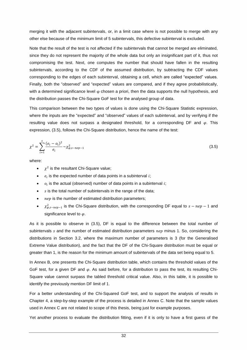
32
merging it with the adjacent subintervals, or, in a limit case where is not possible to merge with any
other else because of the minimum limit of 5 subintervals, this defective subinterval is excluded.
Note that the result of the test is not affected if the subintervals that cannot be merged are eliminated,
since they do not represent the majority of the whole data but only an insignificant part of it, thus not
compromising the test. Next, one computes the number that should have fallen in the resulting
subintervals, according to the CDF of the assumed distribution, by subtracting the CDF values
corresponding to the edges of each subinterval, obtaining a cell, which are called “expected” values.
Finally, both the “observed” and “expected” values are compared, and if they agree probabilistically,
with a determined significance level φ chosen a priori, then the data supports the null hypothesis, and
the distribution passes the Chi-Square GoF test for the analysed group of data.
This comparison between the two types of values is done using the Chi-Square Statistic expression,
where the inputs are the “expected” and “observed” values of each subinterval, and by verifying if the
resulting value does not surpass a designated threshold, for a corresponding DF and 𝜑. This
expression, (3.5), follows the Chi-Square distribution, hence the name of the test:
𝜒2 =∑(𝑒𝑖 − 𝑜𝑖)
2
𝑒𝑖~𝜒𝜑,𝑠−𝑛𝑒𝑝−1
2
𝑠
𝑖=1
(3.5)
where:
𝜒2 is the resultant Chi-Square value;
𝑒𝑖 is the expected number of data points in a subinterval 𝑖;
𝑜𝑖 is the actual (observed) number of data points in a subinterval 𝑖;
𝑠 is the total number of subintervals in the range of the data;
𝑛𝑒𝑝 is the number of estimated distribution parameters;
𝜒𝜑,𝑠−𝑛𝑒𝑝−12 is the Chi-Square distribution, with the corresponding DF equal to 𝑠 − 𝑛𝑒𝑝 − 1 and
significance level to 𝜑.
As it is possible to observe in (3.5), DF is equal to the difference between the total number of
subintervals 𝑠 and the number of estimated distribution parameters 𝑛𝑒𝑝 minus 1. So, considering the
distributions in Section 3.2, where the maximum number of parameters is 3 (for the Generalised
Extreme Value distribution), and the fact that the DF of the Chi-Square distribution must be equal or
greater than 1, is the reason for the minimum amount of subintervals of the data set being equal to 5.
In Annex B, one presents the Chi-Square distribution table, which contains the threshold values of the
GoF test, for a given DF and 𝜑. As said before, for a distribution to pass the test, its resulting Chi-
Square value cannot surpass the tabled threshold critical value. Also, in this table, it is possible to
identify the previously mention DF limit of 1.
For a better understanding of the Chi-Squared GoF test, and to support the analysis of results in
Chapter 4, a step-by-step example of the process is detailed in Annex C. Note that the sample values
used in Annex C are not related to scope of this thesis, being just for example purposes.
Yet another process to evaluate the distribution fitting, even if it is only to have a first guess of the

33
distribution fitted to the data and to outwit some initial cases from the process, is by measuring the
correlation and the Mean Square Error (MSE) between the PDF of the hypothetical distribution and the
histogram of the actual data.
Correlation 𝑐𝑜𝑟𝑟, obtained by (3.6) [EvSk10], is the dependence between two variables 𝑋 and 𝑌,
where a result of 1 means total correlation and 0 represents no correlation between the variables.
𝑐𝑜𝑟𝑟 =∑ (𝑥𝑖 − ��)(𝑦𝑖 − ��)𝑁𝑖=1
√∑ (𝑥𝑖 − ��)2𝑁
𝑖=1 ∑ (𝑦𝑖 − ��)2𝑁
𝑖=1
(3.6)
where:
𝑐𝑜𝑟𝑟 is the correlation value;
𝑥𝑖 and 𝑦𝑖 are the variables to correlate;
�� and �� are mean of the variable to correlate;
𝑁 is the number of samples of each variable.
As for MSE, it measures the average of the squares of the errors, that is, the difference between the
estimator and the estimated, i.e., the PDF of the hypothetical distribution and the histogram of the
evaluated data, respectively. It is calculated by:
휀2 =1
𝑁∑(��𝑖 − 𝑌𝑖)
2𝑁
𝑖=1
(3.7)
where:
휀2 is the MSE;
��𝑖 is the estimated value for the PDF at the centre range of the histogram cell 𝑖;
𝑌𝑖 is the value of the histogram cell 𝑖.
𝑁 is the number of samples of each variable.
One uses the absolute MSE and not the relative MSE due to the fact that the absolute nature of the
MSE is more useful in the direct comparison between the PDF and the histogram of the distribution
and data samples, respectively, because once the distribution value gets too small, the relative MSE
returns very large values, which would disrupt the analysis process, annihilating any good results.
With this approach, it is possible to have a second comparative method of the GoF of the distribution
to the data, the simple visual graphical analysis and the Chi-Square GoF test being the first and third
methods in order, respectively. In terms of precision, obviously, the Chi-Square GoF test is the main
method of analysis; if, for instance, a distribution has a low value of correlation but yet manages to
pass this test, it is considered that the distribution is a good representation of the concerned data
samples.
34
3.4 Data Analysis Model
In order to evaluate the data, a program was developed in MATLAB© to aid in the processing and
calculations required by the methods that have been chosen to use.
In Figure 3.1 and Figure 3.2, a flowchart of the program is illustrated to better understand its
mechanics, a more detailed version of two of its processing blocks being presented in Figure 3.3 and
Figure 3.4, regarding the Chi-Square GoF analysis step and the distribution optimisation block,
respectively, due to their complexity.
Regarding the main program, and focusing on Figure 3.1, first one has to create the basic structures
to store the data and define the default program parameters values. The thresholds, which will add an
upper limit to the sample values, so that the occasional data peaks and anomalies do not disrupt the
tests, are defined here. Also, the minimum amount of data samples that a site must have, so that a
statistical relevant analysis can be done, is also defined in this step. Afterwards, it is needed to import,
individually, the data related to the network parameters to be analysed (delay variation or packet loss),
and store it in the appropriate data structures within the program. These steps were labelled
DEFAULTS and IMPORT, respectively, being depicted in the upper part of Figure 3.1.
The next step consists of searching for data peaks in the imported samples. In PEAK ANALYSIS,
each sample is compared with the previously mentioned threshold, which limits the maximum value
these samples can take. If the sample value is lower than the threshold, then the sample is saved,
otherwise the sample is removed from the stored structure. The number of data peaks each of the
considered sites has is stored in memory, so that an analysis can be done on top of that information.
The core process of the program is DATA ANALYSIS. For each site, first, it is needed to verify that
there is a minimum amount of samples to work with, from the ones left from PEAK ANALYSIS, so that
a reliable statistical result can be obtain with the GoF tests. If it is found that there is a lack of data
samples, the site is considered improper to be analysed, and another site has to be chosen.
Subsequently, after defining the distributions that are going to be evaluated when fitting the data, the
Chi-Square GoF test is performed for each one, with a significance level φ = 95%, and the correlation
and MSE between the distribution PDF and the histogram of the imported data is calculated. Due to
the fact that one of the objectives of this model is to represent all sites with one, or more if it not
possible with one, distribution, then after the DATA ANALYSIS block, an OPTIMISATION process is
made, in order to reassign a distribution to a site based on the results from the previous block.
The Chi-Square test, due to its complexity, is detailed in Figure 3.3. All the steps presented in this
figure are similar to the ones described in the previous Subsection 3.3. To complete the analysis, all
the results of the three computations are taken into account to identify the best distribution that
represents the site.
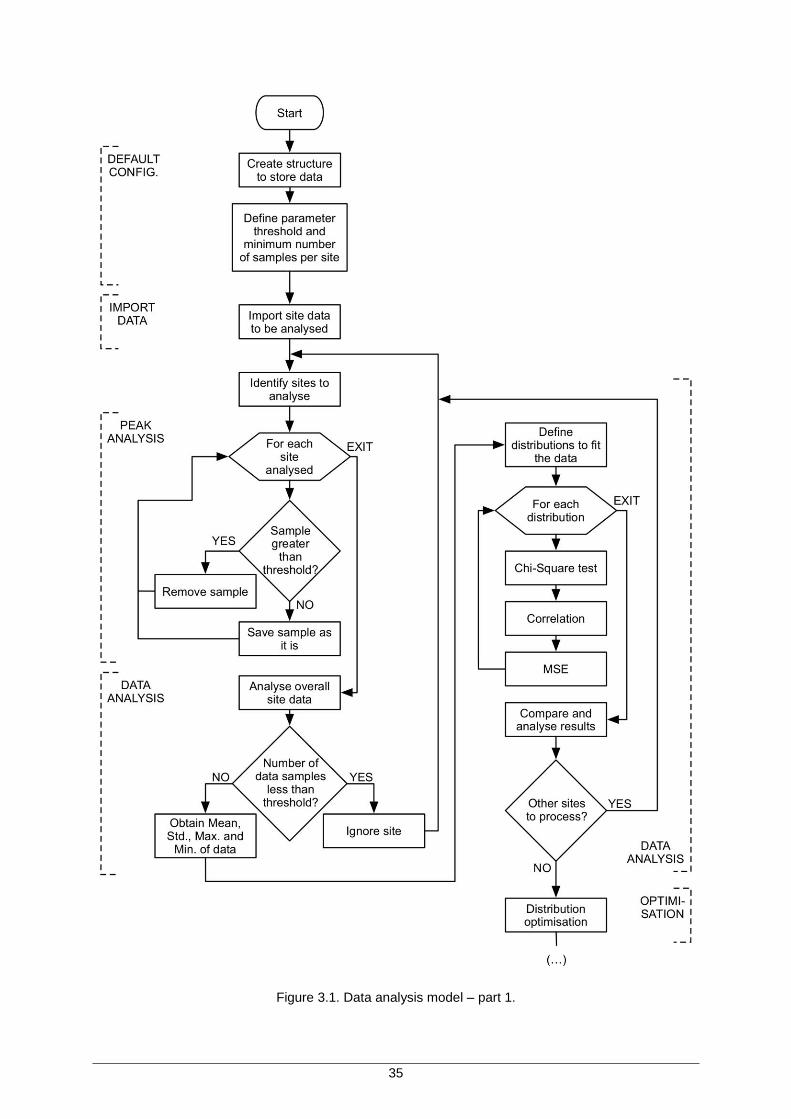
35
Figure 3.1. Data analysis model – part 1.

36
Figure 3.2. Data analysis model – part 2.
In Figure 3.4, one can see a detailed diagram of the process. First, a measure on how many times all
sites processed correspond to each distribution, so that it is possible to adjust other site distributions
to the ones of the majority of sites. Then, for each site, it is examine if the site has been successfully
fitted with one, or more, distributions through the GoF test. If yes, the program searches, within the
group of passed distributions, for one from the top group. If the search is successful, then the
optimised resulting distribution for that site is the one that results from the search. If the search is not
successful, then the parameters that stands out in terms of GoF is the correlation. However, if a site
does not have a single distribution that affirmatively pass the GoF test, then the parameter that stands
out as the most important is, again, the correlation. First of all, if a site does not have a fitted
distribution by the GoF test, and does not have any distribution with a minimum correlation value of
75% (pre-defined within the model) with the sites data, then there is not a single distribution that can
be assign to it.

37
Figure 3.3. Detailed Chi-Square test block.

38
Figure 3.4. Detailed distribution optimisation block.
Still, if there is a distribution that has over 75% of correlation with the data, one can assume that the
respective distribution as some sort of link with it, even though it failed to pass the GoF test. With this,
one can just pick from the over 75% group of distributions, the one that has one of two options: has
higher correlation and belongs to the top of overall distribution; or the one that does not belong to the
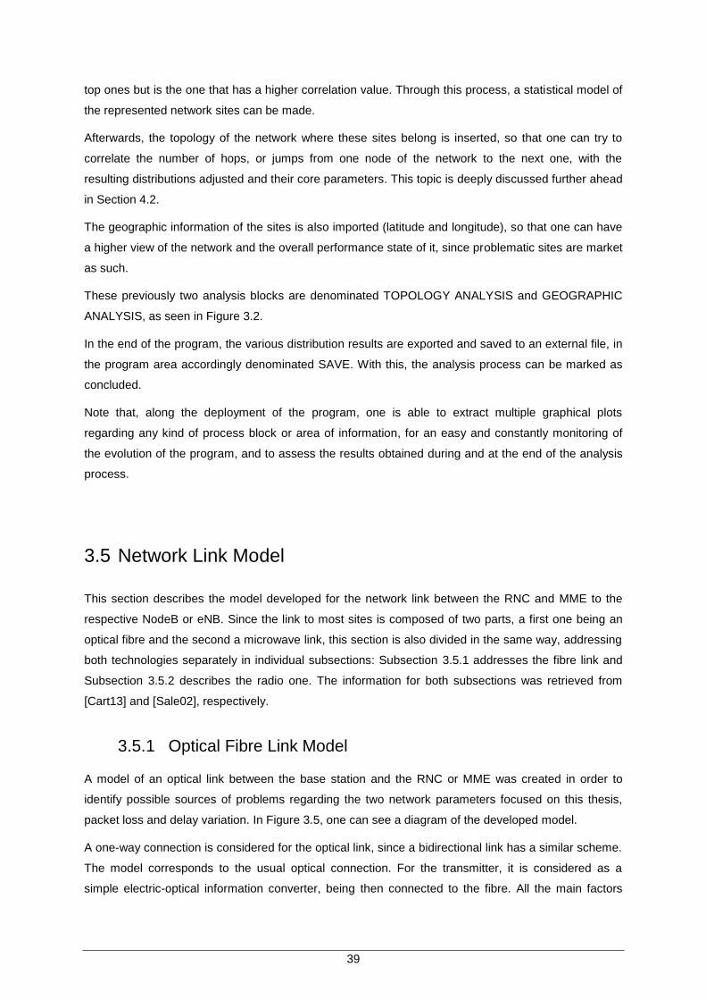
39
top ones but is the one that has a higher correlation value. Through this process, a statistical model of
the represented network sites can be made.
Afterwards, the topology of the network where these sites belong is inserted, so that one can try to
correlate the number of hops, or jumps from one node of the network to the next one, with the
resulting distributions adjusted and their core parameters. This topic is deeply discussed further ahead
in Section 4.2.
The geographic information of the sites is also imported (latitude and longitude), so that one can have
a higher view of the network and the overall performance state of it, since problematic sites are market
as such.
These previously two analysis blocks are denominated TOPOLOGY ANALYSIS and GEOGRAPHIC
ANALYSIS, as seen in Figure 3.2.
In the end of the program, the various distribution results are exported and saved to an external file, in
the program area accordingly denominated SAVE. With this, the analysis process can be marked as
concluded.
Note that, along the deployment of the program, one is able to extract multiple graphical plots
regarding any kind of process block or area of information, for an easy and constantly monitoring of
the evolution of the program, and to assess the results obtained during and at the end of the analysis
process.
3.5 Network Link Model
This section describes the model developed for the network link between the RNC and MME to the
respective NodeB or eNB. Since the link to most sites is composed of two parts, a first one being an
optical fibre and the second a microwave link, this section is also divided in the same way, addressing
both technologies separately in individual subsections: Subsection 3.5.1 addresses the fibre link and
Subsection 3.5.2 describes the radio one. The information for both subsections was retrieved from
[Cart13] and [Sale02], respectively.
3.5.1 Optical Fibre Link Model
A model of an optical link between the base station and the RNC or MME was created in order to
identify possible sources of problems regarding the two network parameters focused on this thesis,
packet loss and delay variation. In Figure 3.5, one can see a diagram of the developed model.
A one-way connection is considered for the optical link, since a bidirectional link has a similar scheme.
The model corresponds to the usual optical connection. For the transmitter, it is considered as a
simple electric-optical information converter, being then connected to the fibre. All the main factors
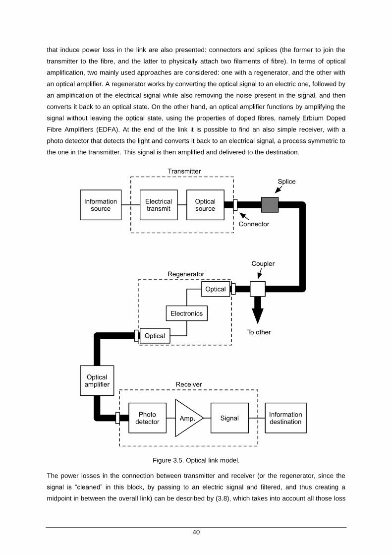
40
that induce power loss in the link are also presented: connectors and splices (the former to join the
transmitter to the fibre, and the latter to physically attach two filaments of fibre). In terms of optical
amplification, two mainly used approaches are considered: one with a regenerator, and the other with
an optical amplifier. A regenerator works by converting the optical signal to an electric one, followed by
an amplification of the electrical signal while also removing the noise present in the signal, and then
converts it back to an optical state. On the other hand, an optical amplifier functions by amplifying the
signal without leaving the optical state, using the properties of doped fibres, namely Erbium Doped
Fibre Amplifiers (EDFA). At the end of the link it is possible to find an also simple receiver, with a
photo detector that detects the light and converts it back to an electrical signal, a process symmetric to
the one in the transmitter. This signal is then amplified and delivered to the destination.
Figure 3.5. Optical link model.
The power losses in the connection between transmitter and receiver (or the regenerator, since the
signal is “cleaned” in this block, by passing to an electric signal and filtered, and thus creating a
midpoint in between the overall link) can be described by (3.8), which takes into account all those loss

41
sources, discriminated in (3.9), and estimates the optical power that reaches the receiver.
𝑃𝑅 [dBm] = 𝑃�� [dBm] − 𝐿𝑇𝑓𝑖𝑏𝑒𝑟[dB] (3.8)
where:
𝑃𝑅 is the average power that reaches the receiver;
𝑃�� is the average power that leaves the transmitter;
𝐿𝑇𝑓𝑖𝑏𝑒𝑟 is the total attenuation suffered by the optical signal;
and,
𝐿𝑇𝑓𝑖𝑏𝑒𝑟[dB]=∑𝛼𝑖𝑙𝑖
𝑁𝑖
𝑖=1
+𝑁𝑆𝐿𝑆 + 𝑁𝐶𝐿𝐶 (3.9)
where:
𝐿𝑇𝑓𝑖𝑏𝑒𝑟 is the total attenuation suffered by the optical signal;
𝑁𝑖 is the number of fibre link sections;
𝛼𝑖 is the attenuation of the fibre section 𝑖;
𝑙𝑖 is the length of the fibre section 𝑖;
𝑁𝑆 is the number of splices in the link;
𝐿𝑆 is the attenuation per splice;
𝑁𝐶 is the number of connector in the link;
𝐿𝐶 is the attenuation per connector.
The average optical power that reaches the receiver is directly connected to the percentage of packets
lost in the link, in the sense that a lower received power needs a more sensitive receiver to guarantee
the same levels of performance. If the power received drops below the minimum required to sustain a
certain degree of performance, the receiver is not able to differentiate the actual signal from
communication noise, leading to the packet being dropped.
3.5.2 Microwave Link Model
The microwave link model, likewise the previous one, can also be depicted as an aggregation of
different major blocks that perform a settled group of tasks. The various building blocks that make it up
are shown in Figure 3.6.
The baseband data traffic, together with the various overhead bytes for signalling, service channels,
and radio control are fed into a multiplexer, where they are combined into an aggregate digital stream,
which is done in the MULDEM (Multiplexer-Demultiplexer) block. Afterwards, this aggregated stream
is condensed into a more efficient bit stream with a reduced bandwidth in the modulator, the MODEM
(Modulator-Demodulator) block. A conversion to an Intermediate Frequency (IF), where amplification
is easier in terms of linearity, and then up converted to Radio Frequency (RF) and fed to the high
power amplifier module in the final stage, is done in the TRANS-RECEIVER. This signal is then fed to
42
the branching unit for connection to the antenna to be transmitted.
On the receiving end of the model, the process is done in the inverse order, where the signal is
converted to IF, demodulated and demuxed, before its information is handled to the final destination.
Figure 3.6. Microwave link model.
As done for the optical link, one can also measure the power loss in a radio link. The general equation
for the optical link, (3.8) is similar,

43
𝑃𝑅 [dBm] = 𝑃�� [dBm] − 𝐿𝑇𝑟𝑎𝑑𝑖𝑜[dB] (3.10)
where:
𝑃𝑅 is the average power that reaches the receiver;
𝑃�� is the average power that leaves the transmitter;
𝐿𝑇𝑟𝑎𝑑𝑖𝑜 is the total attenuation suffered by the microwave signal.
but obviously the attenuation suffered by the radio signal is different:
𝐿𝑇𝑟𝑎𝑑𝑖𝑜[dB]= 𝐿𝐸𝑚𝑖[dB] + 𝐿𝑅𝑒𝑐[dB] − 𝐺𝐸[dBi] − 𝐺𝑅[dBi] − 𝐿0[dB] (3.11)
where:
𝐿𝑇𝑟𝑎𝑑𝑖𝑜 is the total attenuation suffered by the microwave signal;
𝐿𝐸𝑚𝑖 is the attenuation in the emitter waveguide;
𝐿𝑅𝑒𝑐 is the attenuation in the receiver waveguide;
𝐺𝐸 is the emitter antenna gain;
𝐺𝑅 is the receiver antenna gain;
𝐿0 is the free-svariation attenuation.
and
𝐿0 = 32.448 + 20 log10 (𝑑𝑙𝑖𝑛𝑘[km]) + 20 log10(𝑓[MHz]) (3.12)
where:
𝐿0 is the resultant free-svariation attenuation;
𝑑𝑙𝑖𝑛𝑘 is the distance between the transmitting and receiving antennas;
𝑓 is the frequency of the signal transmitted.
In the receiver, the baseband signal is recovered by the demodulator, which, after, detects and
decides, converts the signal in a sequence of bits. Once reconstructed, in the receiver, the sequence
of bits transmitted, one has to identify the signal within it. Is in this process that the power received
affects the packet loss of the inferred link. Like in the optical part, if the signal power received is low,
the noise will overcome the signal, and thus a coherent detection of the bits is not possible, leading to
misconceived frames, that ultimately are discarded, helping increase the percentage of packets lost
within the link.

44

45
Chapter 4
Results Analysis
4 Results Analysis
In Chapter 4, first the scenario is presented in Section 4.1, which is then used to test the developed
model. In Section 4.2, the results for the UMTS part of the scenario are presented, while in Section 4.3
the ones for LTE are shown. To conclude this chapter, in Section 4.4, the theoretical results for the link
model are addressed.
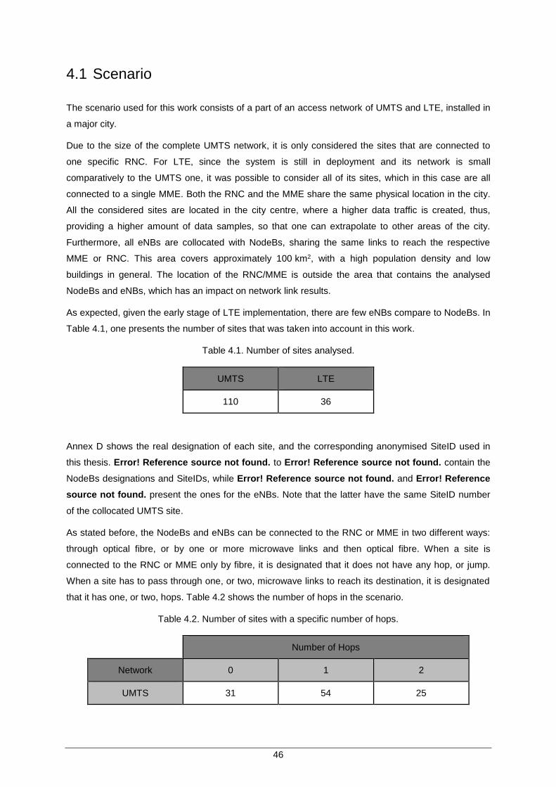
46
4.1 Scenario
The scenario used for this work consists of a part of an access network of UMTS and LTE, installed in
a major city.
Due to the size of the complete UMTS network, it is only considered the sites that are connected to
one specific RNC. For LTE, since the system is still in deployment and its network is small
comparatively to the UMTS one, it was possible to consider all of its sites, which in this case are all
connected to a single MME. Both the RNC and the MME share the same physical location in the city.
All the considered sites are located in the city centre, where a higher data traffic is created, thus,
providing a higher amount of data samples, so that one can extrapolate to other areas of the city.
Furthermore, all eNBs are collocated with NodeBs, sharing the same links to reach the respective
MME or RNC. This area covers approximately 100 km2, with a high population density and low
buildings in general. The location of the RNC/MME is outside the area that contains the analysed
NodeBs and eNBs, which has an impact on network link results.
As expected, given the early stage of LTE implementation, there are few eNBs compare to NodeBs. In
Table 4.1, one presents the number of sites that was taken into account in this work.
Table 4.1. Number of sites analysed.
UMTS LTE
110 36
Annex D shows the real designation of each site, and the corresponding anonymised SiteID used in
this thesis. Error! Reference source not found. to Error! Reference source not found. contain the
NodeBs designations and SiteIDs, while Error! Reference source not found. and Error! Reference
source not found. present the ones for the eNBs. Note that the latter have the same SiteID number
of the collocated UMTS site.
As stated before, the NodeBs and eNBs can be connected to the RNC or MME in two different ways:
through optical fibre, or by one or more microwave links and then optical fibre. When a site is
connected to the RNC or MME only by fibre, it is designated that it does not have any hop, or jump.
When a site has to pass through one, or two, microwave links to reach its destination, it is designated
that it has one, or two, hops. Table 4.2 shows the number of hops in the scenario.
Table 4.2. Number of sites with a specific number of hops.
Number of Hops
Network 0 1 2
UMTS 31 54 25

47
LTE 14 15 7
The data from these sites were obtained through ESAT (Ericsson Stats Analysis Tool), a software that
manages the entire network, and, consequently, all the sites under analysis. One has chosen different
counters and KPIs (Key Performance Indicators) for delay variation and packet loss, for both UMTS
and LTE. In Annex E, it is possible to see the counters and KPIs used to extract the data, and how
they were obtained using the referred tool.
For comparison purposes, one has chosen two ranges of days associated to two different scenarios:
weekdays (Monday to Friday) and weekends (Saturday and Sunday), Table 4.3. The traffic profile and
behaviour experienced by both networks is different for these two scenarios, which motivated their
choice.
Table 4.3. Days evaluated in both scenarios.
Scenario Days
Weekdays 3 to 7 of February, 2014
Weekends 8 and 9 of February, 2014
A time granularity of 15 minutes was used, since it is the smallest one that tool enables.
The number of samples obtained for each parameter, in the respective scenario, depends on the
network, since not all sites have the same data in the seven days. Table 4.4 shows how many
samples were analysed for each network, and for each type of days.
Table 4.4. Number of samples for each parameter for all the scenarios analysed.
UMTS LTE
Parameter Weekdays Weekend Weekdays Weekend
Delay Variation 50 801 20 214 17 329 6 753
Packet Loss 50 803 20 926 17 217 6 909
Concerning UMTS, most of the sites had enough data, with an average of 460 samples per site, per
parameter, resulting in an average of 92 samples per day during weekdays; on the weekend, the
same average value is approximately maintained, for both delay variation and packet loss. Regarding
LTE, the samples are not spread equally over all sites, some sites having around 200 samples for
both parameters during the weekdays (which gives an average of 40 samples per day), and others
having none; during the weekend, it was found that the average number of samples, on the sites with
data, is around 90, which gives a similar samples/day ratio as for weekdays.

48
Finally, one has defined another group of values to be use in the model: the thresholds. There are
three sets of thresholds: the overall performance status in terms of the lost packets and the delay
variation; the minimum amount of samples each site must have to be proper analysed; and the control
of each individual sample to prevent sporadic peaks events. In order to be considered to have a good
performance within each parameter, each site must have its average value below the thresholds of
20 μs and 1%, for delay variation and packet loss, respectively. These values were provided by
Ericsson, as the standard values for both parameters threshold performance. Regarding the minimum
amount of required samples, each site needs a minimum of 80 samples to be eligible for evaluation,
because a lower value wouldn’t provide a reasonable statistical approximation. For the peak status of
each sample, a peak of delay variation sample is considered if it surpasses the value of 100 μs, and a
peak of packet loss data appears when a sample is greater than the threshold value of 15% of packets
lost per unit of time. Both values were obtained by observing the performance thresholds that are
considered. Since those are the values to achieve, the peak thresholds chosen are high enough so
that any sample that reaches them can be safely designated as a peak.
4.2 UMTS Data Analysis
In this section, one shows the results obtained for UMTS, for both weekdays and weekends, through
the Data Analysis Model developed and presented in Section 3.4. In Subsections 4.2.1 and 4.2.2, the
results concerning Delay Variation and Packet Loss are presented, while in Subsection 4.2.3 an
overview of the overall UMTS scenario is given.
4.2.1 Delay Variation
The results of the model can be divided into several parts, each one corresponding to the major
processing blocks that compose the program. The first results come from the analysis of data peaks.
From all samples, one has found 323 delay variation peaks in weekdays, resulting in 0.64% of
samples above the threshold for peak status, and 106 peaks in the weekend, resulting in 0.52% of
peaks.
It is possible to conclude that, even though there are more peaks during weekday, given the higher
number of days, the proportion of peaks does not change, hence, the number of peaks does not
depend on the specific day. Individually, is was possible to verify that, during weekdays, SiteID_98
and SiteID_57 were the worst, with 109 and 57 peaks, representing 40% and 12%, respectively, of the
480 samples each one has, and over the weekend it was SiteID_98, again, and SiteID_107, who
performed worse, with 44 (23%) and 15 (8%) delay variation peaks, respectively. In Figure 4.1, it is
possible to see all NodeBs with the respective peaks, for both scenarios.
A conclusion can be made, regarding SiteID_98, that some problem exists, due to the large amount of
peak samples. In Section 4.4, an analysis on which can be the possible sources of the problem is
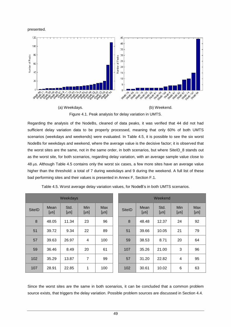
49
presented.
(a) Weekdays. (b) Weekend.
Figure 4.1. Peak analysis for delay variation in UMTS.
Regarding the analysis of the NodeBs, cleaned of data peaks, it was verified that 44 did not had
sufficient delay variation data to be properly processed, meaning that only 60% of both UMTS
scenarios (weekdays and weekends) were evaluated. In Table 4.5, it is possible to see the six worst
NodeBs for weekdays and weekend, where the average value is the decisive factor; it is observed that
the worst sites are the same, not in the same order, in both scenarios, but where SiteID_8 stands out
as the worst site, for both scenarios, regarding delay variation, with an average sample value close to
48 μs. Although Table 4.5 contains only the worst six cases, a few more sites have an average value
higher than the threshold: a total of 7 during weekdays and 9 during the weekend. A full list of these
bad performing sites and their values is presented in Annex F, Section F.1.
Table 4.5. Worst average delay variation values, for NodeB’s in both UMTS scenarios.
Weekdays
Weekend
SiteID Mean [μs]
Std. [μs]
Min [μs]
Max [μs]
SiteID Mean [μs]
Std. [μs]
Min [μs]
Max [μs]
8 48.05 11.34 23 96
8 48.48 12.37 24 92
51 39.72 9.34 22 89
51 39.66 10.05 21 79
57 39.63 26.97 4 100
59 38.53 8.71 20 64
59 36.46 8.49 20 61
107 35.26 21.00 3 96
102 35.29 13.87 7 99
57 31.20 22.82 4 95
107 28.91 22.85 1 100
102 30.61 10.02 6 63
Since the worst sites are the same in both scenarios, it can be concluded that a common problem
source exists, that triggers the delay variation. Possible problem sources are discussed in Section 4.4.
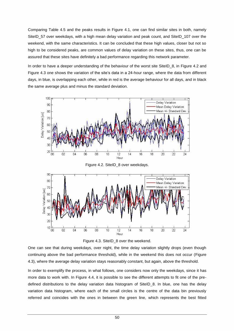
50
Comparing Table 4.5 and the peaks results in Figure 4.1, one can find similar sites in both, namely
SiteID_57 over weekdays, with a high mean delay variation and peak count, and SiteID_107 over the
weekend, with the same characteristics. It can be concluded that these high values, closer but not so
high to be considered peaks, are common values of delay variation on these sites, thus, one can be
assured that these sites have definitely a bad performance regarding this network parameter.
In order to have a deeper understanding of the behaviour of the worst site SiteID_8, in Figure 4.2 and
Figure 4.3 one shows the variation of the site’s data in a 24-hour range, where the data from different
days, in blue, is overlapping each other, while in red is the average behaviour for all days, and in black
the same average plus and minus the standard deviation.
Figure 4.2. SiteID_8 over weekdays.
Figure 4.3. SiteID_8 over the weekend.
One can see that during weekdays, over night, the time delay variation slightly drops (even though
continuing above the bad performance threshold), while in the weekend this does not occur (Figure
4.3), where the average delay variation stays reasonably constant, but again, above the threshold.
In order to exemplify the process, in what follows, one considers now only the weekdays, since it has
more data to work with. In Figure 4.4, it is possible to see the different attempts to fit one of the pre-
defined distributions to the delay variation data histogram of SiteID_8. In blue, one has the delay
variation data histogram, where each of the small circles is the centre of the data bin previously
referred and coincides with the ones in between the green line, which represents the best fitted

51
distribution, in this case being the Generalised Extreme Value distribution.
Figure 4.4. Fitting distributions to SiteID_8’s delay variation data.
In Table 4.6 one can see how that decision was made. Clearly, the Rayleigh distribution is rapidly
excluded, due to exceeding the critical Chi-square value by a large margin and because of the very
low correlation. However, there are a few distributions that do not surpass the critical value and have a
good correlation with the data: Gamma, Generalised Extreme Value, Inverse Gaussian, Log-normal
and Rice. This conclusion can be made also by observing the various plots resulting from these
distributions, where all of them follow, more or less, the behaviour of the delay variation histogram
data. As said when explaining the analysis model, the criterion of selection in these cases (when there
are multiple distributions that pass the test), is the result of the Chi-Square test, where the chosen
distribution is the one that has a lower value.
Table 4.6. Chi-square test, correlation and MSE values for SiteID_8.
Distribution Chi-Square
value Chi-Square critical value
Correlation [%] MSE [× 10−5]
Generalised Extreme Value 44.14 48.60 79.2 5.6
Gamma 44.76 49.80 79.1 5.6
Nakagami 44.83 49.80 78.6 5.6
Inverse Gaussian 48.52 49.80 78.7 5.8
Log-normal 48.60 49.80 78.8 5.8
Rice 49.07 49.80 76.9 6.0
Weibull 55.57 49.80 74.0 6.6
Log-logistic 56.62 49.80 78.0 6.4
Logistic 59.72 49.80 76.2 6.6

52
Rayleigh 262.99 51.00 9.1 0.0
A quick note regarding the Chi-Square critical value: it only changes two times, for the Generalised
Extreme Value distribution and the Rayleigh one, due to the fact that it only depends on the number of
data bins and on the number of the distribution parameters corresponding to the one that it is trying to
fit. So, since the number of data bins is equal for all the distributions in the process, the critical value
only changes if the number of distribution parameters changes, and that only happens for the two
distributions mentioned above.
Still concerning weekdays, by applying the DATA ANALYSIS process block of the program to all of
NodeBs, one reaches the results presented in Table 4.7, where the number of times each distribution
has been chosen to represent a site, through the GoF test, is represented.
Table 4.7. Number of distributions, before the optimisation.
Distribution Number of
occurrences
Generalised Extreme Value 9
Log-logistic 9
Gamma 3
Inverse Gaussian 3
Nakagami 2
Log-normal 1
Weibull 1
Logistic 0
Rayleigh 0
Rice 0
The results in Table 4.7 only account for the sites that have a distribution correctly fitted with the Chi-
Square test. As it can be seen, only 28 of the 110 possible sites passed the GoF test, corresponding
to 25% of the overall scenario. All the others have to be processed through the OPTIMISATION
analysis block of the model, which tries to fit to the remaining sites one of the distributions that have
more occurrences within the GoF result group, which in this case are the Generalised Extreme Value
and the Log-logistic distributions.
The results for the OPTIMISATION block are depicted in Table 4.8, showing the global results for both
types of days.
It is concluded that, independently of the scenario being weekdays or weekends, the UMTS network
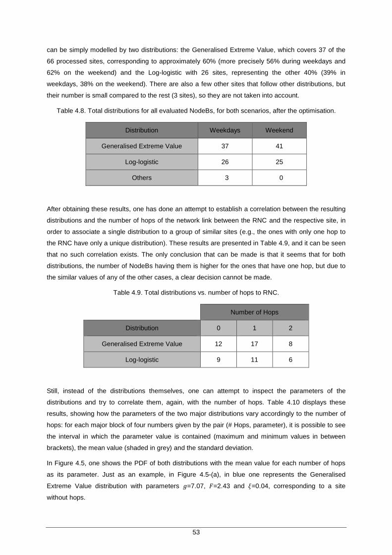
53
can be simply modelled by two distributions: the Generalised Extreme Value, which covers 37 of the
66 processed sites, corresponding to approximately 60% (more precisely 56% during weekdays and
62% on the weekend) and the Log-logistic with 26 sites, representing the other 40% (39% in
weekdays, 38% on the weekend). There are also a few other sites that follow other distributions, but
their number is small compared to the rest (3 sites), so they are not taken into account.
Table 4.8. Total distributions for all evaluated NodeBs, for both scenarios, after the optimisation.
Distribution Weekdays Weekend
Generalised Extreme Value 37 41
Log-logistic 26 25
Others 3 0
After obtaining these results, one has done an attempt to establish a correlation between the resulting
distributions and the number of hops of the network link between the RNC and the respective site, in
order to associate a single distribution to a group of similar sites (e.g., the ones with only one hop to
the RNC have only a unique distribution). These results are presented in Table 4.9, and it can be seen
that no such correlation exists. The only conclusion that can be made is that it seems that for both
distributions, the number of NodeBs having them is higher for the ones that have one hop, but due to
the similar values of any of the other cases, a clear decision cannot be made.
Table 4.9. Total distributions vs. number of hops to RNC.
Number of Hops
Distribution 0 1 2
Generalised Extreme Value 12 17 8
Log-logistic 9 11 6
Still, instead of the distributions themselves, one can attempt to inspect the parameters of the
distributions and try to correlate them, again, with the number of hops. Table 4.10 displays these
results, showing how the parameters of the two major distributions vary accordingly to the number of
hops: for each major block of four numbers given by the pair (# Hops, parameter), it is possible to see
the interval in which the parameter value is contained (maximum and minimum values in between
brackets), the mean value (shaded in grey) and the standard deviation.
In Figure 4.5, one shows the PDF of both distributions with the mean value for each number of hops
as its parameter. Just as an example, in Figure 4.5-(a), in blue one represents the Generalised
Extreme Value distribution with parameters 𝑔=7.07, 𝐹=2.43 and 𝜉=0.04, corresponding to a site
without hops.
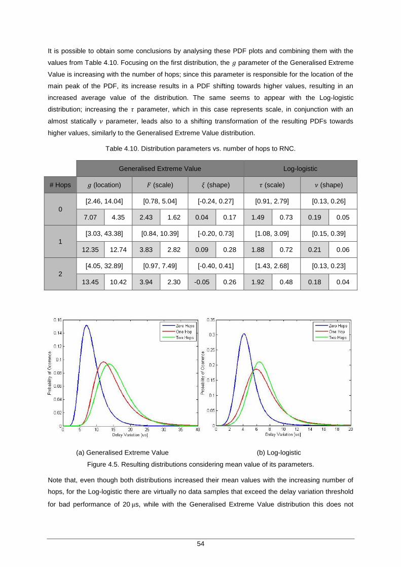
54
It is possible to obtain some conclusions by analysing these PDF plots and combining them with the
values from Table 4.10. Focusing on the first distribution, the 𝑔 parameter of the Generalised Extreme
Value is increasing with the number of hops; since this parameter is responsible for the location of the
main peak of the PDF, its increase results in a PDF shifting towards higher values, resulting in an
increased average value of the distribution. The same seems to appear with the Log-logistic
distribution; increasing the 𝜏 parameter, which in this case represents scale, in conjunction with an
almost statically 𝜈 parameter, leads also to a shifting transformation of the resulting PDFs towards
higher values, similarly to the Generalised Extreme Value distribution.
Table 4.10. Distribution parameters vs. number of hops to RNC.
Generalised Extreme Value Log-logistic
# Hops 𝑔 (location) 𝐹 (scale) 𝜉 (shape) 𝜏 (scale) 𝜈 (shape)
0
[2.46, 14.04] [0.78, 5.04] [-0.24, 0.27] [0.91, 2.79] [0.13, 0.26]
7.07 4.35 2.43 1.62 0.04 0.17 1.49 0.73 0.19 0.05
1
[3.03, 43.38] [0.84, 10.39] [-0.20, 0.73] [1.08, 3.09] [0.15, 0.39]
12.35 12.74 3.83 2.82 0.09 0.28 1.88 0.72 0.21 0.06
2
[4.05, 32.89] [0.97, 7.49] [-0.40, 0.41] [1.43, 2.68] [0.13, 0.23]
13.45 10.42 3.94 2.30 -0.05 0.26 1.92 0.48 0.18 0.04
(a) Generalised Extreme Value (b) Log-logistic
Figure 4.5. Resulting distributions considering mean value of its parameters.
Note that, even though both distributions increased their mean values with the increasing number of
hops, for the Log-logistic there are virtually no data samples that exceed the delay variation threshold
for bad performance of 20 μs, while with the Generalised Extreme Value distribution this does not
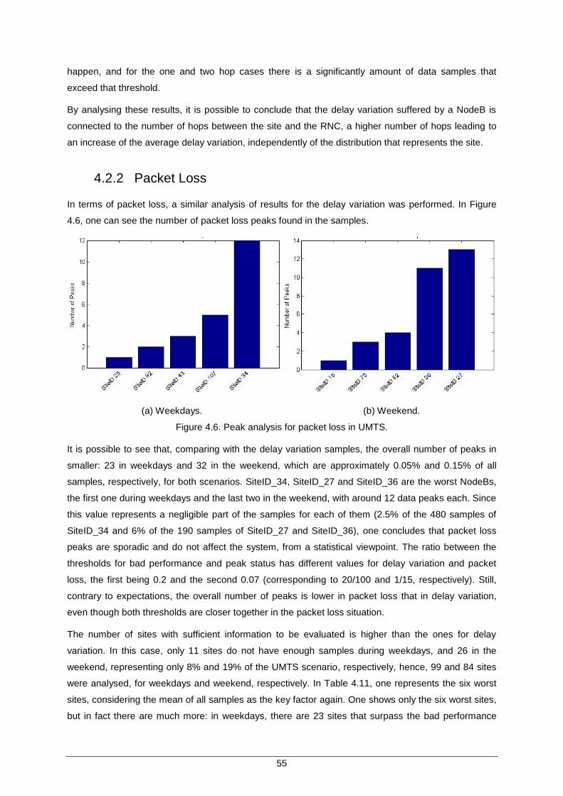
55
happen, and for the one and two hop cases there is a significantly amount of data samples that
exceed that threshold.
By analysing these results, it is possible to conclude that the delay variation suffered by a NodeB is
connected to the number of hops between the site and the RNC, a higher number of hops leading to
an increase of the average delay variation, independently of the distribution that represents the site.
4.2.2 Packet Loss
In terms of packet loss, a similar analysis of results for the delay variation was performed. In Figure
4.6, one can see the number of packet loss peaks found in the samples.
(a) Weekdays. (b) Weekend.
Figure 4.6. Peak analysis for packet loss in UMTS.
It is possible to see that, comparing with the delay variation samples, the overall number of peaks in
smaller: 23 in weekdays and 32 in the weekend, which are approximately 0.05% and 0.15% of all
samples, respectively, for both scenarios. SiteID_34, SiteID_27 and SiteID_36 are the worst NodeBs,
the first one during weekdays and the last two in the weekend, with around 12 data peaks each. Since
this value represents a negligible part of the samples for each of them (2.5% of the 480 samples of
SiteID_34 and 6% of the 190 samples of SiteID_27 and SiteID_36), one concludes that packet loss
peaks are sporadic and do not affect the system, from a statistical viewpoint. The ratio between the
thresholds for bad performance and peak status has different values for delay variation and packet
loss, the first being 0.2 and the second 0.07 (corresponding to 20/100 and 1/15, respectively). Still,
contrary to expectations, the overall number of peaks is lower in packet loss that in delay variation,
even though both thresholds are closer together in the packet loss situation.
The number of sites with sufficient information to be evaluated is higher than the ones for delay
variation. In this case, only 11 sites do not have enough samples during weekdays, and 26 in the
weekend, representing only 8% and 19% of the UMTS scenario, respectively, hence, 99 and 84 sites
were analysed, for weekdays and weekend, respectively. In Table 4.11, one represents the six worst
sites, considering the mean of all samples as the key factor again. One shows only the six worst sites,
but in fact there are much more: in weekdays, there are 23 sites that surpass the bad performance

56
threshold of 1%, while on the weekend there are 22, representing approximately 15% of the whole
network. As with delay variation, a complete list is presented in Annex F, more precisely in Section
F.2. Again, there is not much change between the scenarios, where critical sites maintain themselves
as such, in both scenarios; only SiteID_25 is not part of the critical sites table during the weekend,
suggesting that the problem of this site must be connected to traffic volume, which must change over
the weekend due to a possible lack of users using the system or also a movement of the same users
to another part of the network.
Table 4.11. Worst packet loss average values, for NodeBs in both UMTS scenarios.
Weekdays Weekend
SiteID Mean [%]
Std. [%]
Min [%]
Max [%]
SiteID
Mean [%]
Std. [%]
Min [%]
Max [%]
25 7.25 3.69 0.025 14.58 82 7.76 3.94 0.015 14.85
34 6.92 3.94 0.002 14.80 81 7.22 3.66 0.053 14.89
75 6.73 3.33 0.003 12.93 34 7.09 3.30 0.016 14.93
82 6.72 4.12 0.005 14.64 75 7.07 3.47 0.029 13.95
29 6.13 3.54 0.007 13.16 29 5.54 3.26 0.003 11.93
81 6.04 3.49 0.002 14.58 83 4.00 2.94 0.002 11.55
Observing both Figure 4.7 and Figure 4.8, one can confirm the definitive factor that influences the
behaviour of packet loss during the day: volume of data traffic. As expected, the packet loss
decreases rapidly during night hours, when the amount of users using the system is lower than the
one during the day. Both figures represent the worst sites for the two scenarios, SiteID_25 and
SiteID_82, and the variation of the samples is not different for either of them.
Figure 4.7. SiteID_25 behaviour during weekdays.
In order to reinforce the idea that the packet loss is directly related to the volume of active system

57
users, in Figure 4.9 one can see all the packet loss average values throughout the day, overlapping
each other, of all the sites that exceed the 1% mean threshold during the weekend. From 2 am to
6 am, the average values decrease to an almost acceptable value below the threshold of 1%, due to
the fact that it is night hours, and there are not many users using their mobile devices, as expected.
Figure 4.8. SiteID_82 behaviour during the weekend.
Figure 4.9. Overlapping of packet loss average values on all the worst sites, throughout the 24 hour
day, for both scenarios.
Considering again the process of finding a distribution that can be used for these parameters, which
was the same as before, the final results are showed, already after the optimisation processes, in
Table 4.12.
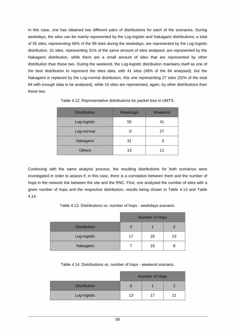
58
In this case, one has obtained two different pairs of distributions for each of the scenarios. During
weekdays, the sites can be mainly represented by the Log-logistic and Nakagami distributions; a total
of 55 sites, representing 56% of the 99 sites during the weekdays, are represented by the Log-logistic
distribution, 31 sites, representing 31% of the same amount of sites analysed, are represented by the
Nakagami distribution, while there are a small amount of sites that are represented by other
distribution than these two. During the weekend, the Log-logistic distribution maintains itself as one of
the best distribution to represent the sites data, with 41 sites (49% of the 84 analysed), but the
Nakagami is replaced by the Log-normal distribution, this one representing 27 sites (32% of the total
84 with enough data to be analysed), while 16 sites are represented, again, by other distributions than
these two.
Table 4.12. Representative distributions for packet loss in UMTS.
Distribution Weekdays Weekend
Log-logistic 55 41
Log-normal 0 27
Nakagami 31 5
Others 13 11
Continuing with the same analysis process, the resulting distributions for both scenarios were
investigated in order to assess if, in this case, there is a correlation between them and the number of
hops in the network link between the site and the RNC. First, one analysed the number of sites with a
given number of hops and the respective distribution, results being shown in Table 4.13 and Table
4.14.
Table 4.13. Distributions vs. number of hops - weekdays scenario.
Number of Hops
Distribution 0 1 2
Log-logistic 17 25 13
Nakagami 7 16 8
Table 4.14. Distributions vs. number of hops - weekend scenario.
Number of Hops
Distribution 0 1 2
Log-logistic 13 17 11
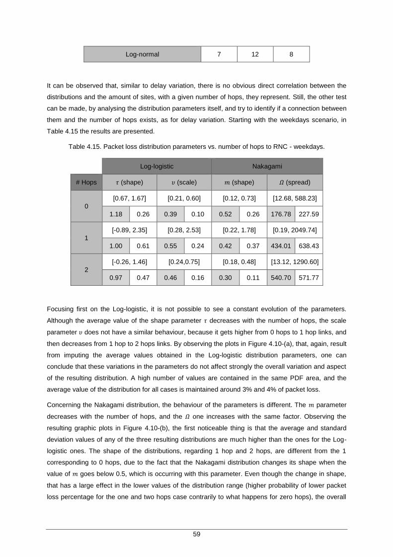
59
Log-normal 7 12 8
It can be observed that, similar to delay variation, there is no obvious direct correlation between the
distributions and the amount of sites, with a given number of hops, they represent. Still, the other test
can be made, by analysing the distribution parameters itself, and try to identify if a connection between
them and the number of hops exists, as for delay variation. Starting with the weekdays scenario, in
Table 4.15 the results are presented.
Table 4.15. Packet loss distribution parameters vs. number of hops to RNC - weekdays.
Log-logistic Nakagami
# Hops 𝜏 (shape) 𝜐 (scale) 𝑚 (shape) 𝛺 (spread)
0
[0.67, 1.67] [0.21, 0.60] [0.12, 0.73] [12.68, 588.23]
1.18 0.26 0.39 0.10 0.52 0.26 176.78 227.59
1
[-0.89, 2.35] [0.28, 2.53] [0.22, 1.78] [0.19, 2049.74]
1.00 0.61 0.55 0.24 0.42 0.37 434.01 638.43
2
[-0.26, 1.46] [0.24,0.75] [0.18, 0.48] [13.12, 1290.60]
0.97 0.47 0.46 0.16 0.30 0.11 540.70 571.77
Focusing first on the Log-logistic, it is not possible to see a constant evolution of the parameters.
Although the average value of the shape parameter 𝜏 decreases with the number of hops, the scale
parameter 𝜐 does not have a similar behaviour, because it gets higher from 0 hops to 1 hop links, and
then decreases from 1 hop to 2 hops links. By observing the plots in Figure 4.10-(a), that, again, result
from imputing the average values obtained in the Log-logistic distribution parameters, one can
conclude that these variations in the parameters do not affect strongly the overall variation and aspect
of the resulting distribution. A high number of values are contained in the same PDF area, and the
average value of the distribution for all cases is maintained around 3% and 4% of packet loss.
Concerning the Nakagami distribution, the behaviour of the parameters is different. The 𝑚 parameter
decreases with the number of hops, and the 𝛺 one increases with the same factor. Observing the
resulting graphic plots in Figure 4.10-(b), the first noticeable thing is that the average and standard
deviation values of any of the three resulting distributions are much higher than the ones for the Log-
logistic ones. The shape of the distributions, regarding 1 hop and 2 hops, are different from the 1
corresponding to 0 hops, due to the fact that the Nakagami distribution changes its shape when the
value of 𝑚 goes below 0.5, which is occurring with this parameter. Even though the change in shape,
that has a large effect in the lower values of the distribution range (higher probability of lower packet
loss percentage for the one and two hops case contrarily to what happens for zero hops), the overall

60
meaning of the sites represented by the Nakagami distribution is that they all suffer from high average
and standard deviation values, putting all of them into the bad performance group of sites.
(a) Log-logistic. (b) Nakagami.
Figure 4.10. Resulting distributions considering the average value of its parameters with different
number of hops, during the weekdays scenario.
Focusing now on the weekend scenario, the results are in Table 4.16. In terms of the Log-logistic
distribution, the same thing as the previous scenario occurs, but this time it is the 𝜐 parameter that has
a continual increasing behaviour with the number of hops, and the values of 𝜏 do not follow a similar
variation. Observing the plots in Figure 4.11-(a) one can conclude that they are very similar to the
ones in Figure 4.10-(a), in terms of distribution parameter values, PDF peak values and in terms of the
average value of the distributions, that are all around the 3% and 4% of packets lost. Thus, the
explanation done for the other previous scenario is maintained here.
Table 4.16. Packet loss distribution parameters vs. number of hops to RNC - weekend.
Log-logistic Log-normal
# Hops 𝜏 (shape) 𝜐 (scale) 𝜂 (shape) 𝜙 (spread)
0
[0.06, 1.76] [0.31, 0.62] [0.84, 1.57] [0.72, 1.04]
1.28 0.46 0.44 0.11 0.84 0.29 0.85 0.13
1
[-0.92, 1.97] [0.33, 0.80] [-0.13, 1.58] [0.58, 1.24]
1.13 0.70 0.52 0.13 0.95 0.57 0.98 0.21
2
[0.07, 2.56] [0.38, 0.84] [-0.83, 1.47] [0.75, 1.76]
1.22 0.79 0.60 0.15 0.61 0.93 1.12 0.40
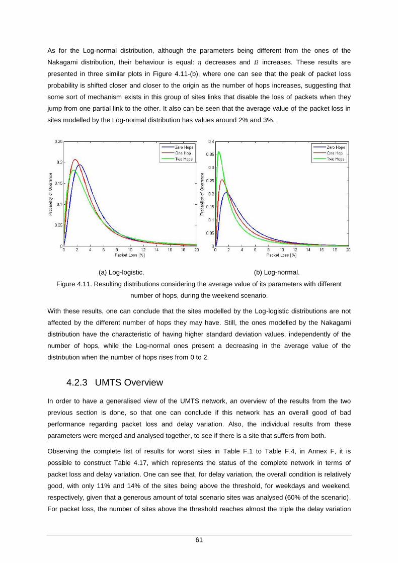
61
As for the Log-normal distribution, although the parameters being different from the ones of the
Nakagami distribution, their behaviour is equal: 𝜂 decreases and 𝛺 increases. These results are
presented in three similar plots in Figure 4.11-(b), where one can see that the peak of packet loss
probability is shifted closer and closer to the origin as the number of hops increases, suggesting that
some sort of mechanism exists in this group of sites links that disable the loss of packets when they
jump from one partial link to the other. It also can be seen that the average value of the packet loss in
sites modelled by the Log-normal distribution has values around 2% and 3%.
(a) Log-logistic. (b) Log-normal.
Figure 4.11. Resulting distributions considering the average value of its parameters with different
number of hops, during the weekend scenario.
With these results, one can conclude that the sites modelled by the Log-logistic distributions are not
affected by the different number of hops they may have. Still, the ones modelled by the Nakagami
distribution have the characteristic of having higher standard deviation values, independently of the
number of hops, while the Log-normal ones present a decreasing in the average value of the
distribution when the number of hops rises from 0 to 2.
4.2.3 UMTS Overview
In order to have a generalised view of the UMTS network, an overview of the results from the two
previous section is done, so that one can conclude if this network has an overall good of bad
performance regarding packet loss and delay variation. Also, the individual results from these
parameters were merged and analysed together, to see if there is a site that suffers from both.
Observing the complete list of results for worst sites in Table F.1 to Table F.4, in Annex F, it is
possible to construct Table 4.17, which represents the status of the complete network in terms of
packet loss and delay variation. One can see that, for delay variation, the overall condition is relatively
good, with only 11% and 14% of the sites being above the threshold, for weekdays and weekend,
respectively, given that a generous amount of total scenario sites was analysed (60% of the scenario).
For packet loss, the number of sites above the threshold reaches almost the triple the delay variation
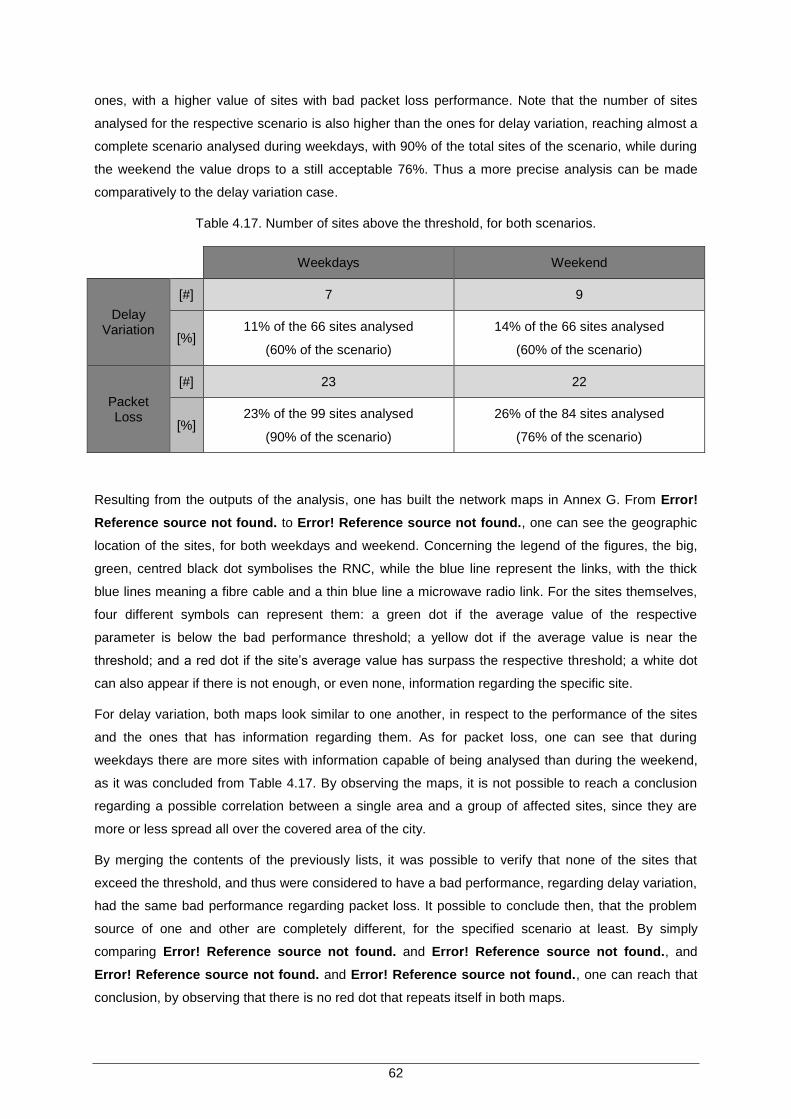
62
ones, with a higher value of sites with bad packet loss performance. Note that the number of sites
analysed for the respective scenario is also higher than the ones for delay variation, reaching almost a
complete scenario analysed during weekdays, with 90% of the total sites of the scenario, while during
the weekend the value drops to a still acceptable 76%. Thus a more precise analysis can be made
comparatively to the delay variation case.
Table 4.17. Number of sites above the threshold, for both scenarios.
Weekdays Weekend
Delay Variation
[#] 7 9
[%] 11% of the 66 sites analysed
(60% of the scenario)
14% of the 66 sites analysed
(60% of the scenario)
Packet Loss
[#] 23 22
[%] 23% of the 99 sites analysed
(90% of the scenario)
26% of the 84 sites analysed
(76% of the scenario)
Resulting from the outputs of the analysis, one has built the network maps in Annex G. From Error!
Reference source not found. to Error! Reference source not found., one can see the geographic
location of the sites, for both weekdays and weekend. Concerning the legend of the figures, the big,
green, centred black dot symbolises the RNC, while the blue line represent the links, with the thick
blue lines meaning a fibre cable and a thin blue line a microwave radio link. For the sites themselves,
four different symbols can represent them: a green dot if the average value of the respective
parameter is below the bad performance threshold; a yellow dot if the average value is near the
threshold; and a red dot if the site’s average value has surpass the respective threshold; a white dot
can also appear if there is not enough, or even none, information regarding the specific site.
For delay variation, both maps look similar to one another, in respect to the performance of the sites
and the ones that has information regarding them. As for packet loss, one can see that during
weekdays there are more sites with information capable of being analysed than during the weekend,
as it was concluded from Table 4.17. By observing the maps, it is not possible to reach a conclusion
regarding a possible correlation between a single area and a group of affected sites, since they are
more or less spread all over the covered area of the city.
By merging the contents of the previously lists, it was possible to verify that none of the sites that
exceed the threshold, and thus were considered to have a bad performance, regarding delay variation,
had the same bad performance regarding packet loss. It possible to conclude then, that the problem
source of one and other are completely different, for the specified scenario at least. By simply
comparing Error! Reference source not found. and Error! Reference source not found., and
Error! Reference source not found. and Error! Reference source not found., one can reach that
conclusion, by observing that there is no red dot that repeats itself in both maps.
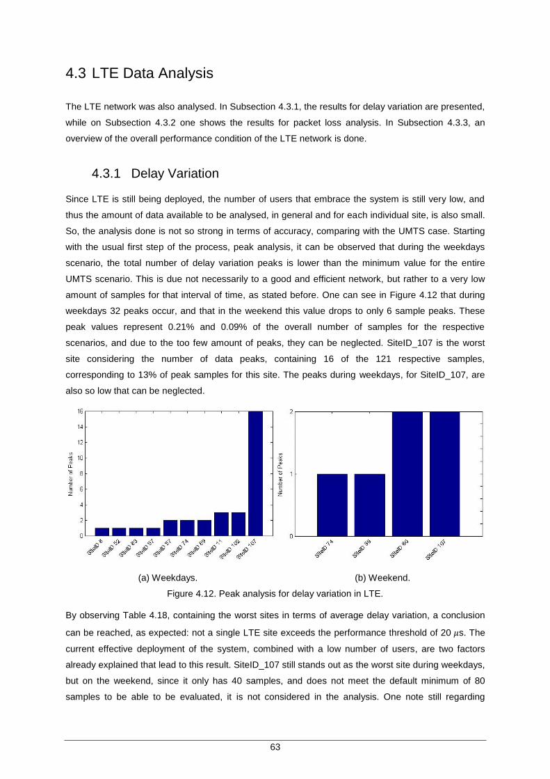
63
4.3 LTE Data Analysis
The LTE network was also analysed. In Subsection 4.3.1, the results for delay variation are presented,
while on Subsection 4.3.2 one shows the results for packet loss analysis. In Subsection 4.3.3, an
overview of the overall performance condition of the LTE network is done.
4.3.1 Delay Variation
Since LTE is still being deployed, the number of users that embrace the system is still very low, and
thus the amount of data available to be analysed, in general and for each individual site, is also small.
So, the analysis done is not so strong in terms of accuracy, comparing with the UMTS case. Starting
with the usual first step of the process, peak analysis, it can be observed that during the weekdays
scenario, the total number of delay variation peaks is lower than the minimum value for the entire
UMTS scenario. This is due not necessarily to a good and efficient network, but rather to a very low
amount of samples for that interval of time, as stated before. One can see in Figure 4.12 that during
weekdays 32 peaks occur, and that in the weekend this value drops to only 6 sample peaks. These
peak values represent 0.21% and 0.09% of the overall number of samples for the respective
scenarios, and due to the too few amount of peaks, they can be neglected. SiteID_107 is the worst
site considering the number of data peaks, containing 16 of the 121 respective samples,
corresponding to 13% of peak samples for this site. The peaks during weekdays, for SiteID_107, are
also so low that can be neglected.
(a) Weekdays. (b) Weekend.
Figure 4.12. Peak analysis for delay variation in LTE.
By observing Table 4.18, containing the worst sites in terms of average delay variation, a conclusion
can be reached, as expected: not a single LTE site exceeds the performance threshold of 20 𝜇s. The
current effective deployment of the system, combined with a low number of users, are two factors
already explained that lead to this result. SiteID_107 still stands out as the worst site during weekdays,
but on the weekend, since it only has 40 samples, and does not meet the default minimum of 80
samples to be able to be evaluated, it is not considered in the analysis. One note still regarding
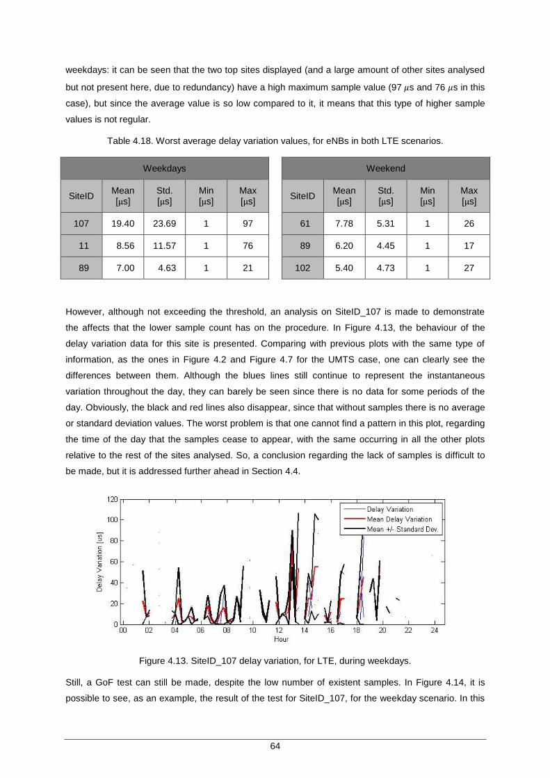
64
weekdays: it can be seen that the two top sites displayed (and a large amount of other sites analysed
but not present here, due to redundancy) have a high maximum sample value (97 𝜇s and 76 𝜇s in this
case), but since the average value is so low compared to it, it means that this type of higher sample
values is not regular.
Table 4.18. Worst average delay variation values, for eNBs in both LTE scenarios.
Weekdays
Weekend
SiteID Mean [μs]
Std. [μs]
Min [μs]
Max [μs]
SiteID Mean [μs]
Std. [μs]
Min [μs]
Max [μs]
107 19.40 23.69 1 97
61 7.78 5.31 1 26
11 8.56 11.57 1 76
89 6.20 4.45 1 17
89 7.00 4.63 1 21
102 5.40 4.73 1 27
However, although not exceeding the threshold, an analysis on SiteID_107 is made to demonstrate
the affects that the lower sample count has on the procedure. In Figure 4.13, the behaviour of the
delay variation data for this site is presented. Comparing with previous plots with the same type of
information, as the ones in Figure 4.2 and Figure 4.7 for the UMTS case, one can clearly see the
differences between them. Although the blues lines still continue to represent the instantaneous
variation throughout the day, they can barely be seen since there is no data for some periods of the
day. Obviously, the black and red lines also disappear, since that without samples there is no average
or standard deviation values. The worst problem is that one cannot find a pattern in this plot, regarding
the time of the day that the samples cease to appear, with the same occurring in all the other plots
relative to the rest of the sites analysed. So, a conclusion regarding the lack of samples is difficult to
be made, but it is addressed further ahead in Section 4.4.
Figure 4.13. SiteID_107 delay variation, for LTE, during weekdays.
Still, a GoF test can still be made, despite the low number of existent samples. In Figure 4.14, it is
possible to see, as an example, the result of the test for SiteID_107, for the weekday scenario. In this
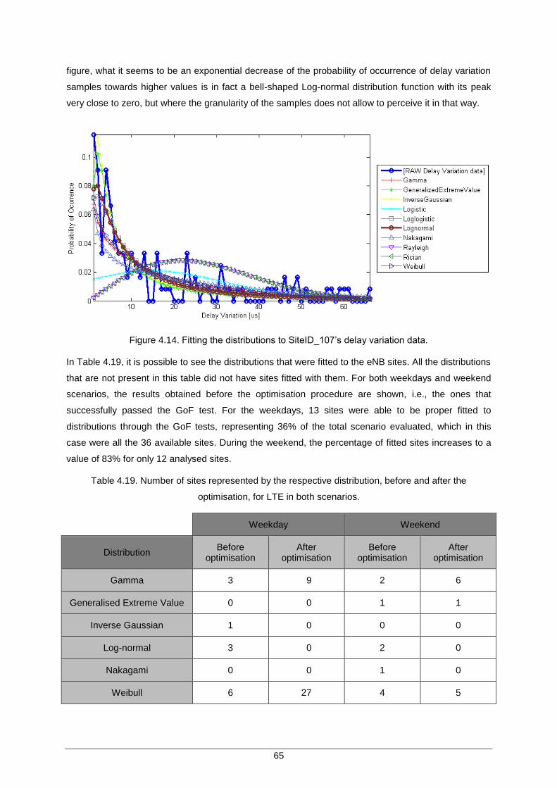
65
figure, what it seems to be an exponential decrease of the probability of occurrence of delay variation
samples towards higher values is in fact a bell-shaped Log-normal distribution function with its peak
very close to zero, but where the granularity of the samples does not allow to perceive it in that way.
Figure 4.14. Fitting the distributions to SiteID_107’s delay variation data.
In Table 4.19, it is possible to see the distributions that were fitted to the eNB sites. All the distributions
that are not present in this table did not have sites fitted with them. For both weekdays and weekend
scenarios, the results obtained before the optimisation procedure are shown, i.e., the ones that
successfully passed the GoF test. For the weekdays, 13 sites were able to be proper fitted to
distributions through the GoF tests, representing 36% of the total scenario evaluated, which in this
case were all the 36 available sites. During the weekend, the percentage of fitted sites increases to a
value of 83% for only 12 analysed sites.
Table 4.19. Number of sites represented by the respective distribution, before and after the
optimisation, for LTE in both scenarios.
Weekday Weekend
Distribution Before
optimisation After
optimisation Before
optimisation After
optimisation
Gamma 3 9 2 6
Generalised Extreme Value 0 0 1 1
Inverse Gaussian 1 0 0 0
Log-normal 3 0 2 0
Nakagami 0 0 1 0
Weibull 6 27 4 5

66
After applying the optimisation process, Table 4.19, it is observed that, for both scenarios, the Gamma
and Weibull distributions exceed as the majority of distributions fitted, resulting that one can made a
similar analysis ahead, for the weekdays and weekend sample values.
Considering now the resulting distributions after the optimisation, only for weekday since it has more
data to work with. A comparison between them and the number of hops is made, again, to find the
desired correlation between the two factors.
Table 4.20. Distributions vs. number of hops - weekdays scenario.
Number of Hops
Distribution 0 1 2
Gamma 3 4 2
Weibull 11 12 4
Also again, the results are not conclusive, since one has a dispersed number of fitted distributions
throughout all of the different number of hops, and they are not focused on only one. Still, the
recurrent comparison of the distributions parameters with the number of hops can still be made. The
results of this comparison are presented in Table 4.21, for the two resultant distributions obtained for
the weekdays scenario.
Table 4.21. Distribution parameters vs. number of hops to the MME.
Gamma Weibull
# Hops 𝑘 (shape) 𝜃 (scale) 𝜆 (scale) 𝑑 (shape)
0
[1.47, 2.17] [2.23, 5.04] [1.86, 8.30] [0.83, 1.65]
1.88 0.32 3.19 1.60 3.47 2.17 1.19 0.30
1
[1.41, 3,62] [0.46, 2.89] [1.78, 17.28] [0.82, 1.73]
2.38 1.13 1.65 1.22 4.33 4.73 1.29 0.32
2
[1.91, 2.61] [1.23, 2.46] [1.89, 6.46] [1.00, 1.32]
2.26 0.5 1.48 0.87 3.97 2.06 1.18 0.13
Using the average values of the parameters for each different number of link hops, the set of PDF
plots corresponding to the respective distributions are presented in Figure 4.15.
Regarding the Gamma distribution, by observing both the group of plots and the parameter values, it
can be concluded that the major change occurs in the transition from the 0 hops to the 1 hop case,
namely due to the decrease of the 𝜃 parameter, which represents the scale of the distribution and
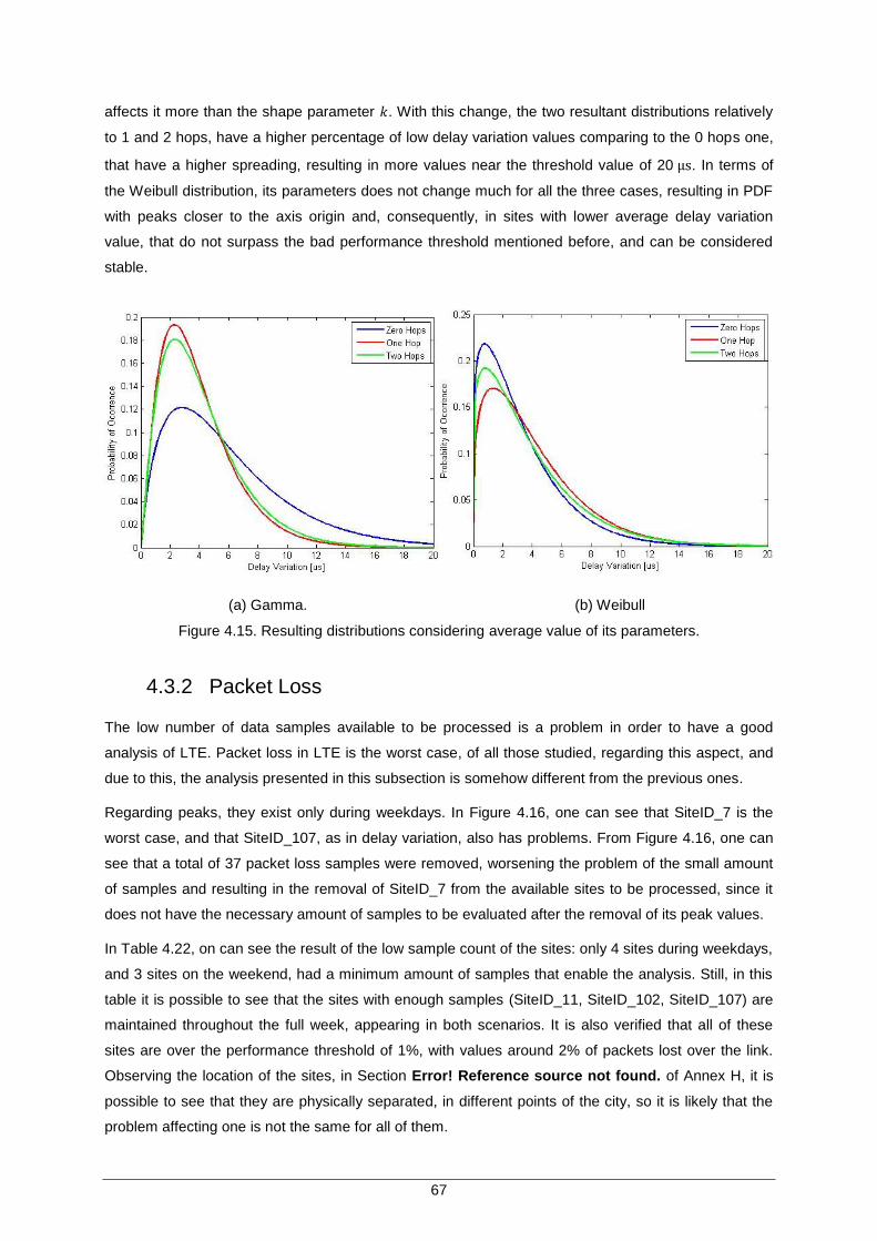
67
affects it more than the shape parameter 𝑘. With this change, the two resultant distributions relatively
to 1 and 2 hops, have a higher percentage of low delay variation values comparing to the 0 hops one,
that have a higher spreading, resulting in more values near the threshold value of 20 μs. In terms of
the Weibull distribution, its parameters does not change much for all the three cases, resulting in PDF
with peaks closer to the axis origin and, consequently, in sites with lower average delay variation
value, that do not surpass the bad performance threshold mentioned before, and can be considered
stable.
(a) Gamma. (b) Weibull
Figure 4.15. Resulting distributions considering average value of its parameters.
4.3.2 Packet Loss
The low number of data samples available to be processed is a problem in order to have a good
analysis of LTE. Packet loss in LTE is the worst case, of all those studied, regarding this aspect, and
due to this, the analysis presented in this subsection is somehow different from the previous ones.
Regarding peaks, they exist only during weekdays. In Figure 4.16, one can see that SiteID_7 is the
worst case, and that SiteID_107, as in delay variation, also has problems. From Figure 4.16, one can
see that a total of 37 packet loss samples were removed, worsening the problem of the small amount
of samples and resulting in the removal of SiteID_7 from the available sites to be processed, since it
does not have the necessary amount of samples to be evaluated after the removal of its peak values.
In Table 4.22, on can see the result of the low sample count of the sites: only 4 sites during weekdays,
and 3 sites on the weekend, had a minimum amount of samples that enable the analysis. Still, in this
table it is possible to see that the sites with enough samples (SiteID_11, SiteID_102, SiteID_107) are
maintained throughout the full week, appearing in both scenarios. It is also verified that all of these
sites are over the performance threshold of 1%, with values around 2% of packets lost over the link.
Observing the location of the sites, in Section Error! Reference source not found. of Annex H, it is
possible to see that they are physically separated, in different points of the city, so it is likely that the
problem affecting one is not the same for all of them.
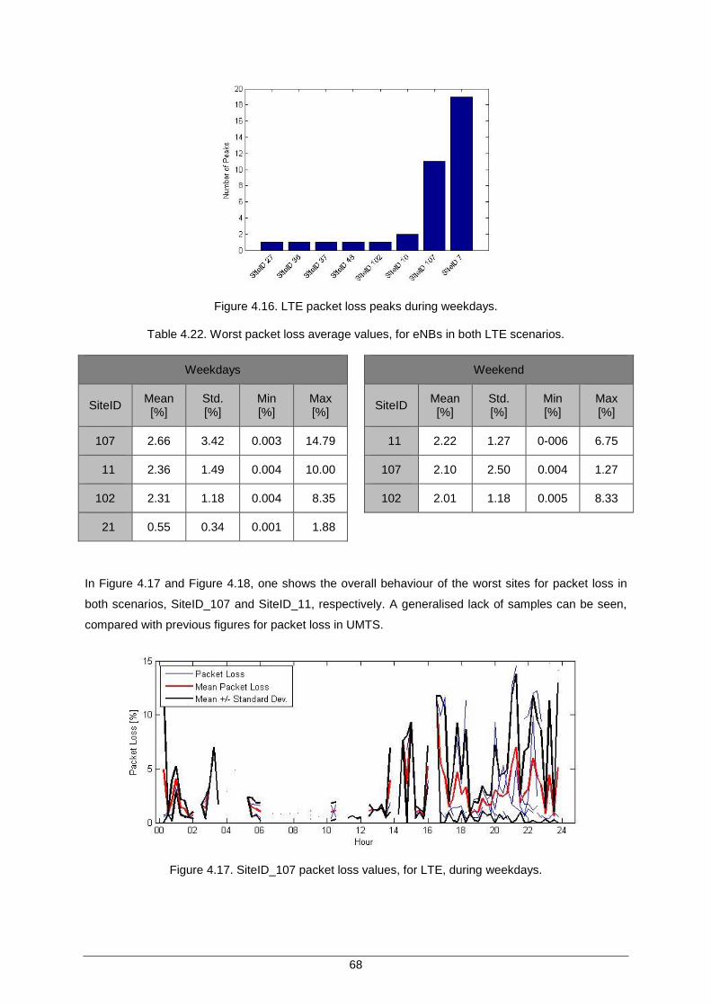
68
Figure 4.16. LTE packet loss peaks during weekdays.
Table 4.22. Worst packet loss average values, for eNBs in both LTE scenarios.
Weekdays Weekend
SiteID Mean [%]
Std. [%]
Min [%]
Max [%]
SiteID
Mean [%]
Std. [%]
Min [%]
Max [%]
107 2.66 3.42 0.003 14.79 11 2.22 1.27 0-006 6.75
11 2.36 1.49 0.004 10.00 107 2.10 2.50 0.004 1.27
102 2.31 1.18 0.004 8.35 102 2.01 1.18 0.005 8.33
21 0.55 0.34 0.001 1.88
In Figure 4.17 and Figure 4.18, one shows the overall behaviour of the worst sites for packet loss in
both scenarios, SiteID_107 and SiteID_11, respectively. A generalised lack of samples can be seen,
compared with previous figures for packet loss in UMTS.
Figure 4.17. SiteID_107 packet loss values, for LTE, during weekdays.
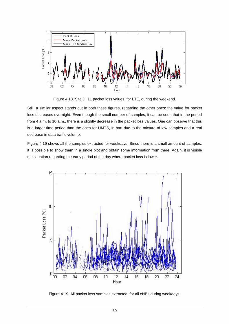
69
Figure 4.18. SiteID_11 packet loss values, for LTE, during the weekend.
Still, a similar aspect stands out in both these figures, regarding the other ones: the value for packet
loss decreases overnight. Even though the small number of samples, it can be seen that in the period
from 4 a.m. to 10 a.m., there is a slightly decrease in the packet loss values. One can observe that this
is a larger time period than the ones for UMTS, in part due to the mixture of low samples and a real
decrease in data traffic volume.
Figure 4.19 shows all the samples extracted for weekdays. Since there is a small amount of samples,
it is possible to show them in a single plot and obtain some information from there. Again, it is visible
the situation regarding the early period of the day where packet loss is lower.
Figure 4.19. All packet loss samples extracted, for all eNBs during weekdays.
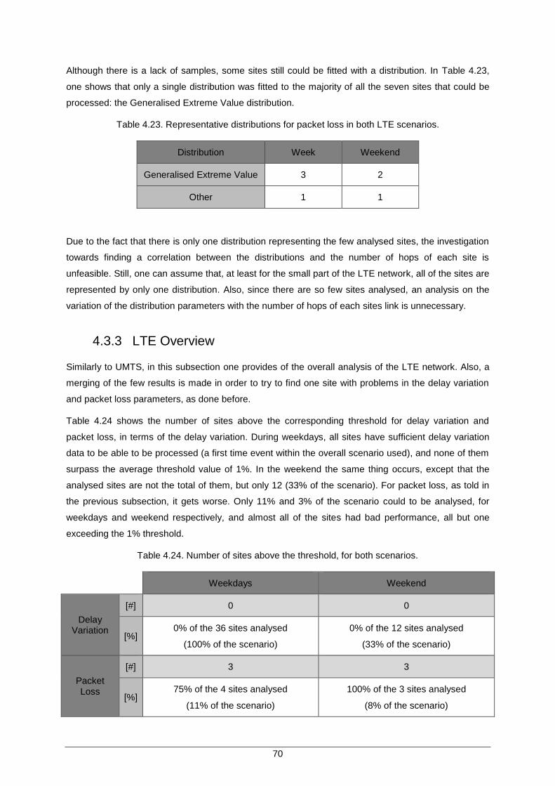
70
Although there is a lack of samples, some sites still could be fitted with a distribution. In Table 4.23,
one shows that only a single distribution was fitted to the majority of all the seven sites that could be
processed: the Generalised Extreme Value distribution.
Table 4.23. Representative distributions for packet loss in both LTE scenarios.
Distribution Week Weekend
Generalised Extreme Value 3 2
Other 1 1
Due to the fact that there is only one distribution representing the few analysed sites, the investigation
towards finding a correlation between the distributions and the number of hops of each site is
unfeasible. Still, one can assume that, at least for the small part of the LTE network, all of the sites are
represented by only one distribution. Also, since there are so few sites analysed, an analysis on the
variation of the distribution parameters with the number of hops of each sites link is unnecessary.
4.3.3 LTE Overview
Similarly to UMTS, in this subsection one provides of the overall analysis of the LTE network. Also, a
merging of the few results is made in order to try to find one site with problems in the delay variation
and packet loss parameters, as done before.
Table 4.24 shows the number of sites above the corresponding threshold for delay variation and
packet loss, in terms of the delay variation. During weekdays, all sites have sufficient delay variation
data to be able to be processed (a first time event within the overall scenario used), and none of them
surpass the average threshold value of 1%. In the weekend the same thing occurs, except that the
analysed sites are not the total of them, but only 12 (33% of the scenario). For packet loss, as told in
the previous subsection, it gets worse. Only 11% and 3% of the scenario could to be analysed, for
weekdays and weekend respectively, and almost all of the sites had bad performance, all but one
exceeding the 1% threshold.
Table 4.24. Number of sites above the threshold, for both scenarios.
Weekdays Weekend
Delay Variation
[#] 0 0
[%] 0% of the 36 sites analysed
(100% of the scenario)
0% of the 12 sites analysed
(33% of the scenario)
Packet Loss
[#] 3 3
[%] 75% of the 4 sites analysed
(11% of the scenario)
100% of the 3 sites analysed
(8% of the scenario)
71
This information was also used to create the network performance map for LTE, which is presented in
Annex H, where it is possible to see the geographical maps of the sites, coloured correspondingly to
the performance status of each one. The legend of the map is the same as for the ones for the UMTS
case: blue lines represent the links (the ones with higher line width are fibre links, and the thinner ones
are microwave radio links); green, yellow and red coloured dots are the sites with good, near bad, and
bad performance, respectively; white dots are sites with no information; and lastly, the green black-
centred dot is the location of the MME where all eNBs are connected. By observing the figures in
Annex H, and Table 4.18 and Table 4.22, it can be conclude that only one site has problems regarding
delay variation and packet loss, and that site is SiteID_107, resulting in the only critical site existing in
the overall LTE scenario analysed.
It can be concluded that as far as delay variation is concerned, the LTE network does not constitute a
problem. A similar statement cannot be confirmed, or denied, for packet loss, since the amount of data
analysed does not have enough statistical significance.
4.4 Network Link Model Analysis
In this section, a theoretical analysis of the network link model is made. Its main characteristics and
components that result in possible sources of the problems that affect the analysed network are
investigated and compared with the obtained results.
Concerning the optical fibre link model, presented in Subsection 3.5.1, and delay variation, there are
several blocks in the model that can be possible problems sources. Still, one of the blocks that do not
contribute to the delay variation is the fibre itself, since it only adds delay to the propagation of the
signal, not delay variation. Considering a typical value of 1.6 for the refractive index of the fibre core
[Cart13], light travels approximately at 1.9 × 10⁸ m/s through the optical link. So, it can be considered
that for each kilometre of fibre, a delay of approximately 5 μs is added to the transmission of the signal.
If the signal transmitted from a NodeB/eNB to a RNC/MME always travels through the same network
path, there is no delay variation, but if this does not occur, a variation in the signal delay will arise due
to the different travelled times resulting from the different network path.
Delay variation in the packets comes from the various nodes in the network, either fibre-to-fibre or
fibre-to-radio. The processing suffered by the packets inside these nodes results in different delays for
each packet, due to the internal analysis that need to be done in terms of, e.g., routing or buffering,
then resulting in delay variation in the receiver. This means that a site with a link that has more hops
has a higher probability of suffering from delay variation, which is supported by the results obtained for
UMTS and LTE. The results in Figure 4.5, for UMTS, show that when the number of hops increases,
the average value of the distribution, and consequently of the delay variation, also increases. In Figure
4.15, the number of hops does not influence delay variation; this is the LTE case, for which there is a

72
low amount of sites with data, hence, the lack of a correlation.
Another source of delay variation in the fibre link are the transmitter, regenerator and receiver. Since
these blocks have to convert the information signal from an electrical state to an optical one, and vice-
versa, the amount of required time depends on the type of packet to process, resulting in variation in
the overall delay of the signal from its source to its destination.
Concerning the possible sources for packet loss problems, in the fibre link, one of the main reasons of
packet loss is a systematic excessive power loss of the transmitted signal. As explained in Subsection
3.5.1, through (3.8) and (3.9), if an extra attenuation occurs, that has not been taken into account at
the time of the link design, like bending losses, deformations in the fibre or bad coupled connectors,
the signal may not have sufficient power to be detected by the receiver, thus, its packets, or some of
its bits, are lost. If by mischance the lost bits are the ones that compose the checksum packet header
(which works as a safety procedure that assures that all data was perfectly received), the packet can
be discarded, since the checksum value is not equivalent to the packet received.
Another possible source of packet loss in the fibre link is when congestion occurs inside one of the
network nodes. If a packet, for some reason, cannot be stored or transmitted by a node, the packet is
discarded, resulting, as one could expect, in an increasing value of lost packets.
Also, a packet can be discarded, and consequently lost, if an excessive latency in the transmission
occurs. One could try to correlate the results for packet loss and delay variation to verify this, but as
seen in the previous sections, almost all the analysed sites do not suffer from bad performance in both
parameters at the same time.
Regarding the microwave radio link, the major difference is that the signal is propagated through the
air. The same considerations regarding power loss also apply here, where the significant difference is
in terms of the attenuations that a signal can suffer propagating over the air, that are far more
unpredictable than the ones that occur inside a fibre, e.g., if an object stands in between the
transmitting and receiving antennas. If the link is not properly designed, simple changes in weather
conditions can affect (depending on frequency) the transmitted signal in terms of fading and power
loss, having also other implications in terms of available signal modulation, and consequently affect
the packets lost along the way.
The results in terms of bit errors, congestion and latency described for the optical link are also applied
to the microwave radio one, because all those factors may also occur here, since bit errors depend on
how the signal is affected throughout the path, and congestion and latency can exist inside the trans-
receiver module. Furthermore, another factor that may imply packet loss, and which is not present in
the optical link, is the link capacity. The high capacity of fibre links can cope with the large volume of
data traffic, thus not being a problem, but this is no longer the case for a radio link, where the capacity
of the link is much smaller, possible being unable to accommodate all the requested data traffic.
In terms of delay variation in a microwave link, the processing time inside the module is also a factor.
The multiplexing and modulation procedures inside the MULDEM and MODEM respectively, and their
inverse processes, are all time consuming. But again, these processes do not have a constant

73
processing time, since they depend on the amount of data that is requested to be transmitted. With
this, one can again formulate that the higher the number of link hops a site has, the higher the average
delay variation of that site is.
A quick note regarding the delay relative to the free space transmission of the microwave links. Since
the microwave sites are located near each other inside the city, the distance between most of them
never surpass the 300 m, except for a couple of cases. Taking this into account, it can be seen that
the delay of the signal never surpasses 1 μs between the transmitter and receiver sites, and thus is
possible to be neglected.
To conclude, a factor that can compromise all processing blocks is the bad parameterisation and
configuration of the transmitting and receiving devices, e.g., in terms of memory buffers, if a buffer is
mistakenly configured to be small, congestion will be constantly occurring, leading to packet loss.

74

75
Chapter 5
Conclusions
5 Conclusions
In this chapter, conclusions are presented, as well as a list of possible paths to take in future work.
76
The objective of this thesis consisted in the investigation of real UMTS and LTE networks, and to
model two specific and crucial parameters: delay variation and packet loss. The critical links being
inside a network, both parameters were measure in the connection between the site and its
corresponding controller (NodeB and RNC for UMTS, and eNB and MME for LTE). Also, possible
sources of both these problems were to be identified through a model of the links in the networks.
In order to give a brief introduction on the subject, a historical view on both UMTS and LTE is first
presented in Chapter 1.
A deep evaluation of the procedures and main components of both systems is needed for a better
understanding of the problem at hand, and why it has to be analysed, which is the focus of Chapter 2.
This analysis included the elaboration of several lists containing the worst sites in terms of the two
parameters analysed, and the fitting of a statistical distribution to each parameter data, extracted from
the NodeBs and eNBs presented in the network. Afterwards, an optimisation procedure was
performed, with the objective of modelling delay variation and packet loss with the same distribution, in
order to predict the behaviour of the parameters throughout time.
Two scenarios were considered in the analysis, regarding two different types of days during a full
week: weekdays and weekend. In terms of the number of sites to analyse, in UMTS there were 110
while in LTE there were only 36.
In order to evaluate the scenarios, an analysis program was developed in MATLAB©, which can be
found in Chapter 3. Its core is a distribution fitting algorithm, based on the Chi-Square GoF test, that
tries to fit one of the pre-defined ten distributions.
Chapter 4 presents the analysis of results. For the UMTS network, regarding delay variation during
the weekdays, it is found that of all the 66 sites that have sufficient associated data for a proper
statistical analysis, 7 surpass the threshold of 20 μs that was defined as the one that a site could not
exceed if considered to have good delay variation performance. These 7 sites correspond to 11% of
all processed sites, which are 60% of the total number of sites in the network. During the weekend, 9
sites exceed the threshold, corresponding to 14%.
With respect to the packet loss in UMTS, it is concluded that 23 sites were above the threshold for bad
performance during weekdays, which in this case was considered to be 1% of lost packets. This group
of sites corresponds to 23% of the 99 sites with enough information to be processed, representing
90% of the total number of sites. In terms of packet loss on the weekend, the number of sites is
similar, 22, but they represent a larger amount of the number of sites analysed, which in this case was
84 sites, i.e., 76%.
Regarding LTE the delay variation for both weekdays and weekend, presents an amount of sites that
surpasses the performance threshold equal to zero. During weekdays, all sites had enough samples
to be analysed. Still, in the weekend, the number of analysed sites decreases to 12, which
corresponds to 33%.
As for packet loss in LTE a problem appeared, since there was a lack of samples for all the sites in the

77
overall scenario. Still, some results could still be collected. During weekdays, it was found that 3 sites
were considered in bad performance, since they all exceeded the threshold. However, only 4 sites of
the 36 possible had enough data to be properly analysed, resulting in 11% of the total processed
scenario. Regarding the weekend, the situation did not change, where of the 3 sites able to be
analysed, 8% of the total, all of them surpass the 1% threshold.
Chapter 4 also contains the results regarding the fitting of distributions to delay variation and packet
loss. For delay variation in UMTS, the Generalised Extreme Value and Log-logistic distributions are
the ones that fit the majority of sites, in both weekdays and weekend. Regarding packet loss in the
same system, the Log-logistic is the one with the most recurrent distribution, together with the
Nakagami one, for weekdays. In the weekend, the Log-logistic distribution is still one of the top fitted
distributions, but this time the Nakagami distribution gives way for the Log-normal distribution to
represent a large group of sites also.
In terms of LTE it is concluded that the Gamma and Weibull distributions are the ones that best fit
delay variation, while for packet loss the Generalised Extreme Value distribution is the best, in both
cases for weekdays and weekend.
The number of hops in the link, connecting the site to the RNC or MME, has a significant impact on
with the delay variation experienced in it. Possible problem sources are identified for packet loss and
delay variation for both links, where the processing time in the node is the factor that has the greater
effect in delay variation, whether packet loss is more affected through the loss of signal power in the
link between transmitter and receiver ends.
Although the objectives of the thesis were accomplished, the analysis in this work has some
limitations, namely in the amount of samples processed, which for the LTE case were significantly low.
If it was possible to have more data samples for both parameters, a more precise analysis, and
accuracy would have been possible.
As for future work, one could correlate more information with these two parameters. For instance, with
information regarding traffic profiles, a conclusion could be reach on how the different types of data
traffic are affected by delay variation or packet loss. Since data traffic has different priorities, one can
expect that the packets with highest priority do not suffer from packet loss, or delay variation for that
matter, since they are prioritised in the processing inside a network node. Another possible work is to
have more information regarding the real network links, in terms of hardware and the actual devices
they are composed of, so that it could be discriminate the path that a packet travels from the site to the
RNC, or MME, delay variation problems being probed. Finally, one could also optimise the program,
so that it runs in real time and could return results instantaneously, and apply it to the complete
network, for a continuous, and more precise, evaluation of the problem.

78
79
Annex A
Statistical Distributions
A Annex A - Statistical Distributions
This annex portraits a graphical representation of the PDF and CDF of all the distributions used in this
thesis, for a proper evaluation of their similarities and differences.

80
Figure A.1 to Figure A.10 present the PDFs and CDFs of all the distributions used within this thesis.
(a) PDF. (b) CDF.
Figure A.1. Gamma distribution.
(a) PDF. (b) CDF.
Figure A.2. Generalised Extreme Value distribution.
(a) PDF. (b) CDF.
Figure A.3. Inverse Gaussian distribution.
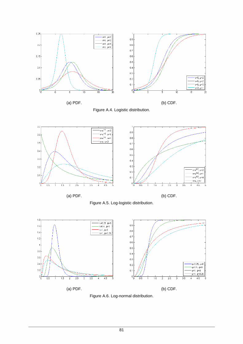
81
(a) PDF. (b) CDF.
Figure A.4. Logistic distribution.
(a) PDF. (b) CDF.
Figure A.5. Log-logistic distribution.
(a) PDF. (b) CDF.
Figure A.6. Log-normal distribution.
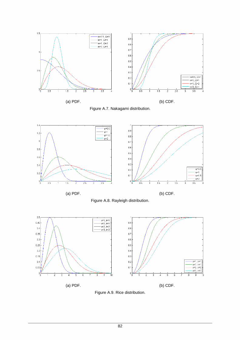
82
(a) PDF. (b) CDF.
Figure A.7. Nakagami distribution.
(a) PDF. (b) CDF.
Figure A.8. Rayleigh distribution.
(a) PDF. (b) CDF.
Figure A.9. Rice distribution.
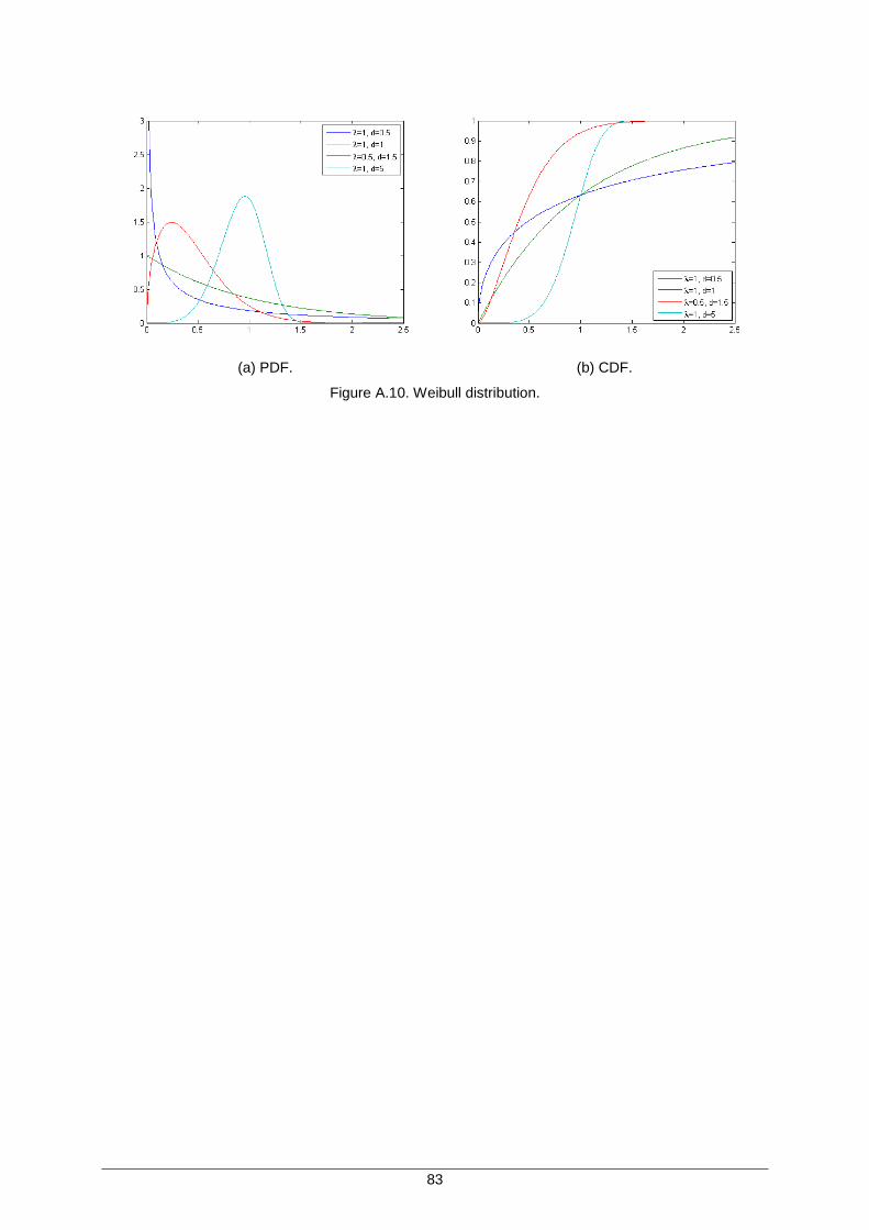
83
(a) PDF. (b) CDF.
Figure A.10. Weibull distribution.

84
85
Annex B
Chi-Square Distribution Table
B Annex B - Chi-Square Distribution Table
This annex presents the Chi-Square distribution table, the basis for the Chi-Square GoF test used in
this thesis.

86
Table B.1. Chi Square distribution table.
𝐷𝐹 𝜒.9952 𝜒.990
2 𝜒.9752 𝜒.950
2 𝜒.9002 𝜒.100
2 𝜒.0502 𝜒.025
2 𝜒.0102 𝜒.005
2
1 0.000 0.000 0.001 0.004 0.016 2.706 3.841 5.024 6.635 7.879 2 0.010 0.020 0.051 0.103 0.211 4.605 5.991 7.378 9.210 10.597 3 0.072 0.115 0.216 0.352 0.584 6.251 7.815 9.348 11.345 12.838 4 0.207 0.297 0.484 0.711 1.064 7.779 9.488 11.143 13.277 14.860 5 0.412 0.554 0.831 1.145 1.610 9.236 11.070 12.833 15.086 16.750
6 0.676 0.872 1.237 1.635 2.204 10.645 12.592 14.449 16.812 18.548 7 0.989 1.239 1.690 2.167 2.833 12.017 14.067 16.013 18.475 20.278 8 1.344 1.646 2.180 2.733 3.490 13.362 15.507 17.535 20.090 21.955 9 1.735 2.088 2.700 3.325 4.168 14.684 16.919 19.023 21.666 23.589 10 2.156 2.558 3.247 3.940 4.865 15.987 18.307 20.483 23.209 25.188
11 2.603 3.053 3.816 4.575 5.578 17.275 19.675 21.920 24.725 26.757 12 3.074 3.571 4.404 5.226 6.304 18.549 21.026 23.337 26.217 28.300 13 3.565 4.107 5.009 5.892 7.042 19.812 22.362 24.736 27.688 29.819 14 4.075 4.660 5.629 6.571 7.790 21.064 23.685 26.119 29.141 31.319 15 4.601 5.229 6.262 7.261 8.547 22.307 24.996 27.488 30.578 32.801
16 5.142 5.812 6.908 7.962 9.312 23.542 26.296 28.845 32.000 34.267 17 5.697 6.408 7.564 8.672 10.085 24.769 27.587 30.191 33.409 35.718 18 6.265 7.015 8.231 9.390 10.865 25.989 28.869 31.526 34.805 37.156 19 6.844 7.633 8.907 10.117 11.651 27.204 30.144 32.852 36.191 38.582 20 7.434 8.260 9.591 10.851 12.443 28.412 31.410 34.170 37.566 39.997
21 8.034 8.897 10.283 11.591 13.240 29.615 32.671 35.479 38.932 41.401 22 8.643 9.542 10.982 12.338 14.041 30.813 33.924 36.781 40.289 42.796 23 9.260 10.196 11.689 13.091 14.848 32.007 35.172 38.076 41.638 44.181 24 9.886 10.856 12.401 13.848 15.659 33.196 36.415 39.364 42.980 45.559 25 10.520 11.524 13.120 14.611 16.473 34.382 37.652 40.646 44.314 46.928
26 11.160 12.198 13.844 15.379 17.292 35.563 38.885 41.923 45.642 48.290 27 11.808 12.879 14.573 16.151 18.114 36.741 40.113 43.195 46.963 49.645 28 12.461 13.565 15.308 16.928 18.939 37.916 41.337 44.461 48.278 50.993 29 13.121 14.256 16.047 17.708 19.768 39.087 42.557 45.722 49.588 52.336 30 13.787 14.953 16.791 18.493 20.599 40.256 43.773 46.979 50.892 53.672
40 20.707 22.164 24.433 26.509 29.051 51.805 55.758 59.342 63.691 66.766 50 27.991 29.707 32.357 34.764 37.689 63.167 67.505 71.420 76.154 79.490 60 35.534 37.485 40.482 43.188 46.459 74.397 79.082 83.298 88.379 91.952 70 43.275 45.442 48.758 51.739 55.329 85.527 90.531 95.023 100.425 104.215
80 51.172 53.540 57.153 60.391 64.278 96.578 101.879 106.629 112.329 116.321 90 59.196 61.754 65.647 69.126 73.291 107.565 113.145 118.136 124.116 128.299 100 67.328 70.065 74.222 77.929 82.358 118.498 124.342 129.561 135.807 140.169
Figure B.1. The shaded area is equal to 𝜑 for 𝜒2 = 𝜒1−𝜑2 .

87
Annex C
Chi-Square GoF Example Test
C Annex C - Chi-Square GoF Example Test
One presents an example of fitting a Normal distribution to a data set, using the Chi-Square GoF test
to verify that the distribution fits the data.
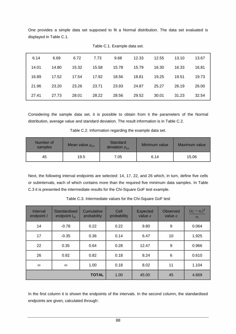
88
One provides a simple data set supposed to fit a Normal distribution. The data set evaluated is
displayed in Table C.1.
Table C.1. Example data set.
6.14 6.69 6.72 7.73 9.68 12.33 12.55 13.10 13.67
14.01 14.80 15.32 15.58 15.78 15.79 16.30 16.33 16.81
16.89 17.52 17.54 17.92 18.56 18.81 19.25 19.51 19.73
21.96 23.20 23.26 23.71 23.93 24.87 25.27 26.19 26.00
27.41 27.73 28.01 28.22 28.56 29.52 30.01 31.23 32.54
Considering the sample data set, it is possible to obtain from it the parameters of the Normal
distribution, average value and standard deviation. The result information is in Table C.2.
Table C.2. Information regarding the example data set.
Number of samples
Mean value 𝜇𝑒𝑥 Standard
deviation 𝜎𝑒𝑥 Minimum value Maximum value
45 19.5 7.05 6.14 15.06
Next, the following interval endpoints are selected: 14, 17, 22, and 26 which, in turn, define five cells
or subintervals, each of which contains more than the required five minimum data samples. In Table
C.3 it is presented the intermediate results for the Chi-Square GoF test example.
Table C.3. Intermediate values for the Chi-Square GoF test
Interval endpoint 𝑙
Standardised endpoint 𝑙𝑠𝑡
Cumulative probability
Cell probability
Expected value 𝑒
Observed value 𝑜
(𝑒𝑖 − 𝑜𝑖)2
𝑒𝑖
14 -0.78 0.22 0.22 9.80 9 0.064
17 -0.35 0.36 0.14 6.47 10 1.925
22 0.35 0.64 0.28 12.47 9 0.966
26 0.92 0.82 0.18 8.24 6 0.610
∞ ∞ 1.00 0.18 8.02 11 1.104
TOTAL 1.00 45.00 45 4.669
In the first column it is shown the endpoints of the intervals. In the second column, the standardised
endpoints are given, calculated through:

89
𝑙𝑠𝑡 =𝑙 − 𝜇𝑒𝑥𝜎𝑒𝑥
(C.1)
where:
𝑙𝑠𝑡 is the interval standardised endpoint;
𝑙 is the interval endpoint;
𝜇𝑒𝑥 is the average value of the data sample set;
𝜎𝑒𝑥 is the standard deviation of the data sample set.
In the third column, the respective cumulative values are presented, obtained from the usual Normal
tables. For example, for the first endpoint (14), it is done as it is shown in (C.2).
𝑃19.5,7.05(14) = 𝑁𝑜𝑟𝑚𝑎𝑙 (14 − 19.5
7.05) = 𝑁𝑜𝑟𝑚𝑎𝑙(−0.78) = 0.22 (C.2)
Then, it is obtain in column four, the lagged differences of the cumulative values, which constitute the
individual cell areas under the assumed Normal distribution. By simply multiplying each cell area by
the total amount of samples, equal to 45, and since each area is the probability that any sample
element falls in the corresponding cell, the result product yields the expected number of elements 𝑒 in
each cell according to the assumed distribution.
Finally, it is processed the observed 𝑜 and expected 𝑒 values, of each cell, through the statistic
formula given by (3.5), which results in:
𝜒2 =∑(𝑒𝑖 − 𝑜𝑖)
2
𝑒𝑖
5
𝑖=1
= 4.67 < 𝜒0.95,22 = 5.99 (C.3)
The Chi-Square statistic value of 4.67 is smaller than the Chi-Square threshold table value of 5.99 for
DF=5-2-1=2 and a 95% significance level, so we can assume that the distribution of the population
originating the data set is 𝑁𝑜𝑟𝑚𝑎𝑙 (19.5, 7.05).

90

91
Annex D
Sites List
D Annex D - Sites List (Confidential)
In this annex one presents a map of the sites in Luanda, as well as their names and designations
given by Ericsson Portugal.

92
93
Annex E
Counters and KPI’s
E Annex E - Counters and KPI’s (Confidential)
This annex provides information regarding the counters and KPI’s, advised by Ericsson to be used in
this work. All the material was removed from ESAT.

94

95
Annex F
UMTS List of Worst Sites
F Annex F - UMTS List of Worst Sites
This annex contains the complete list of the worst sites in UMTS, and the daily behaviour of the top
five cases, regarding delay variation and packet loss, for both scenarios.
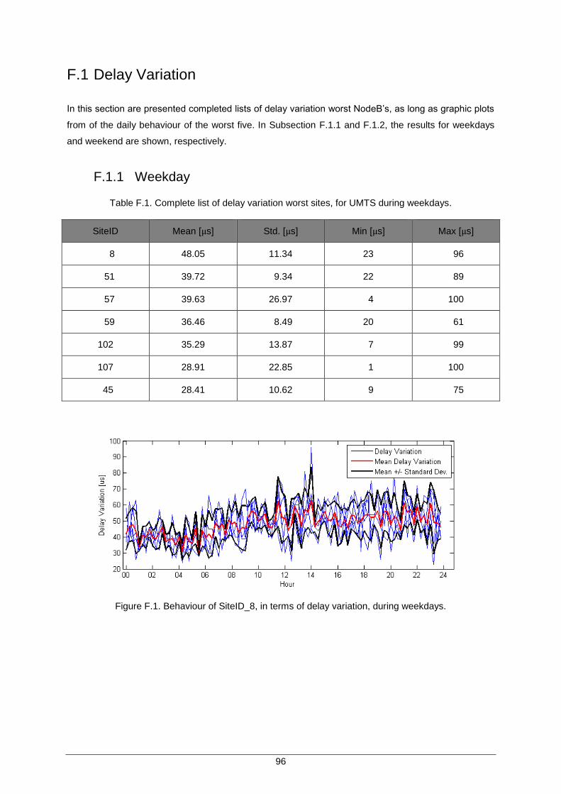
96
F.1 Delay Variation
In this section are presented completed lists of delay variation worst NodeB’s, as long as graphic plots
from of the daily behaviour of the worst five. In Subsection F.1.1 and F.1.2, the results for weekdays
and weekend are shown, respectively.
F.1.1 Weekday
Table F.1. Complete list of delay variation worst sites, for UMTS during weekdays.
SiteID Mean [μs] Std. [μs] Min [μs] Max [μs]
8 48.05 11.34 23 96
51 39.72 9.34 22 89
57 39.63 26.97 4 100
59 36.46 8.49 20 61
102 35.29 13.87 7 99
107 28.91 22.85 1 100
45 28.41 10.62 9 75
Figure F.1. Behaviour of SiteID_8, in terms of delay variation, during weekdays.
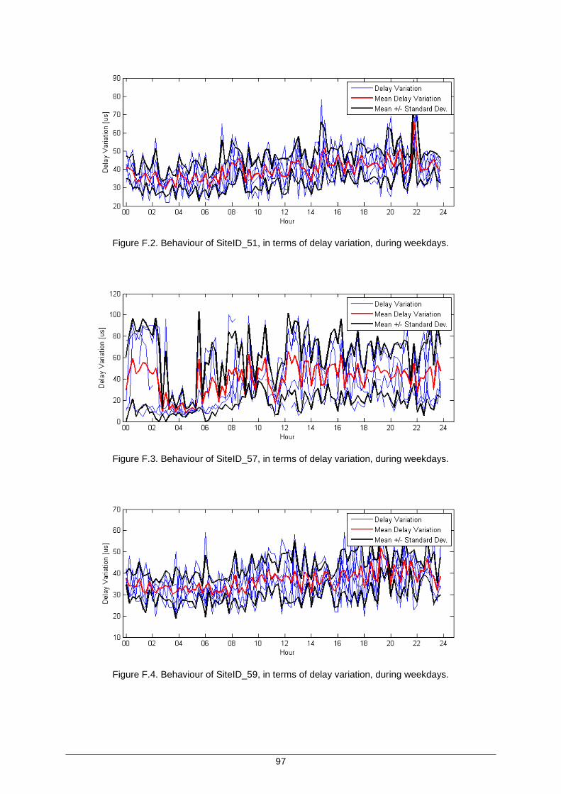
97
Figure F.2. Behaviour of SiteID_51, in terms of delay variation, during weekdays.
Figure F.3. Behaviour of SiteID_57, in terms of delay variation, during weekdays.
Figure F.4. Behaviour of SiteID_59, in terms of delay variation, during weekdays.

98
Figure F.5. Behaviour of SiteID_102, in terms of delay variation, during weekdays.
F.1.2 Weekend
Table F.2. Complete list of delay variation worst sites, for UMTS during the weekend.
SiteID Mean [μs] Std. [μs] Min [μs] Max [μs]
8 48.48 12.37 24 82
51 39.66 10.05 21 79
59 38.53 8.71 20 64
107 35.26 21.00 3 96
57 31.20 22.82 4 95
102 30.61 10.02 6 63
45 26.79 10.18 7 57
65 20.13 7.86 5 41
89 20.06 3.67 11 32
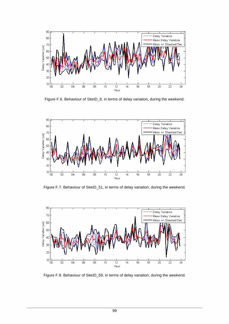
99
Figure F.6. Behaviour of SiteID_8, in terms of delay variation, during the weekend.
Figure F.7. Behaviour of SiteID_51, in terms of delay variation, during the weekend.
Figure F.8. Behaviour of SiteID_59, in terms of delay variation, during the weekend.
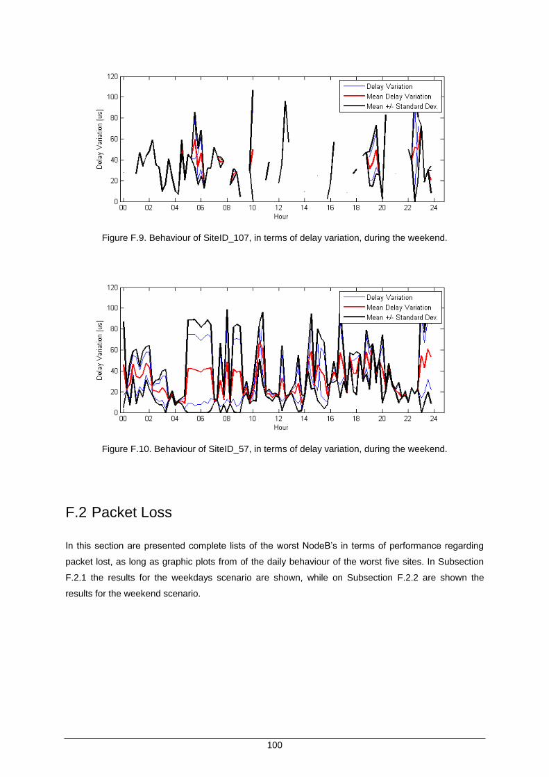
100
Figure F.9. Behaviour of SiteID_107, in terms of delay variation, during the weekend.
Figure F.10. Behaviour of SiteID_57, in terms of delay variation, during the weekend.
F.2 Packet Loss
In this section are presented complete lists of the worst NodeB’s in terms of performance regarding
packet lost, as long as graphic plots from of the daily behaviour of the worst five sites. In Subsection
F.2.1 the results for the weekdays scenario are shown, while on Subsection F.2.2 are shown the
results for the weekend scenario.

101
F.2.1 Weekday
Table F.3. Complete list of packet loss worst sites, for UMTS during weekdays.
SiteID Mean [%] Std. [%] Min [%] Max [%]
25 7.25 3.69 0.016 14.58
34 6.92 3.93 0.002 14.81
75 6.73 3.33 0.003 12.93
82 6.72 4.12 0.005 14.65
29 6.13 3.45 0.007 13.16
81 6.04 3.49 0.002 14.59
53 4.49 2.36 0.006 8.74
17 4.38 2.09 0.007 7.91
16 3.95 1.72 0.616 8.30
47 3.77 2.52 0.002 9.74
44 3.74 2.09 0.002 8.25
83 3.48 2.87 0.004 12.28
1 2.89 1.90 0.001 9.22
2 2.85 2.19 0.003 8.54
3 2.46 1.51 0.003 6.59
72 2.17 1.75 0.001 9.00
43 1.90 2.84 0.002 14.71
42 1.77 1.40 0.002 6.40
55 1.73 1.73 0.001 9.67
56 1.57 1.23 0.002 6.53
4 1.56 1.49 0.003 7.55
40 1.44 1.31 0.001 6.84
18 1.00 1.05 0.002 5.26
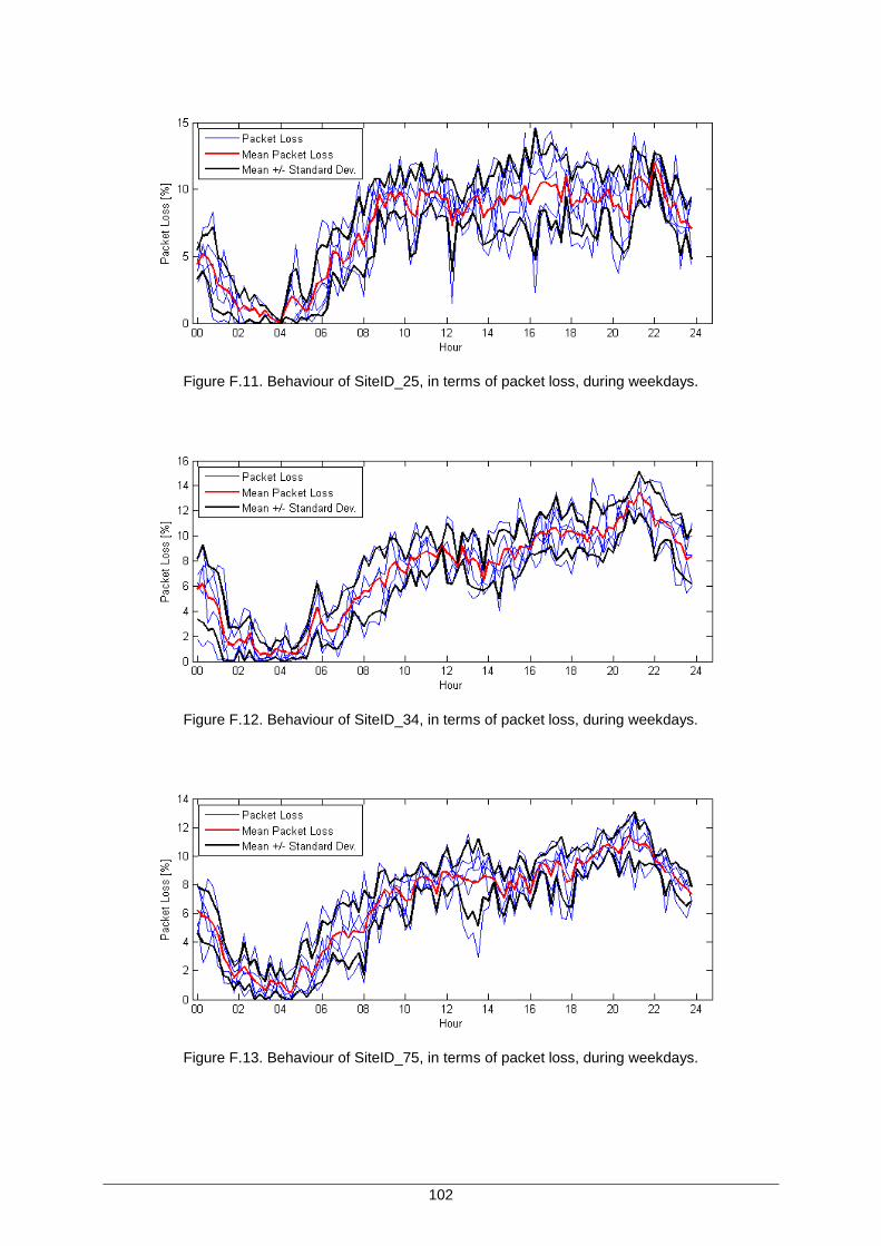
102
Figure F.11. Behaviour of SiteID_25, in terms of packet loss, during weekdays.
Figure F.12. Behaviour of SiteID_34, in terms of packet loss, during weekdays.
Figure F.13. Behaviour of SiteID_75, in terms of packet loss, during weekdays.
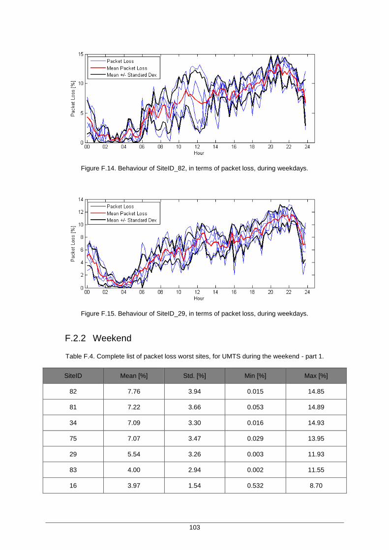
103
Figure F.14. Behaviour of SiteID_82, in terms of packet loss, during weekdays.
Figure F.15. Behaviour of SiteID_29, in terms of packet loss, during weekdays.
F.2.2 Weekend
Table F.4. Complete list of packet loss worst sites, for UMTS during the weekend - part 1.
SiteID Mean [%] Std. [%] Min [%] Max [%]
82 7.76 3.94 0.015 14.85
81 7.22 3.66 0.053 14.89
34 7.09 3.30 0.016 14.93
75 7.07 3.47 0.029 13.95
29 5.54 3.26 0.003 11.93
83 4.00 2.94 0.002 11.55
16 3.97 1.54 0.532 8.70

104
Table F.5. Complete list of packet loss worst sites, for UMTS during the weekend - part 2.
SiteID Mean [%] Std. [%] Min [%] Max [%]
17 3.88 2.16 0.006 7.38
53 3.86 2.24 0.003 7.22
48 3.43 2.47 0.007 9.96
44 2.91 1.64 0.023 7.72
21 2.88 1.53 0.233 9.27
72 2.80 1.86 0.006 9.47
55 2.73 2.15 0.002 8.66
2 2.73 1.88 0.003 7.32
46 2.55 2.01 0.001 6.65
3 2.03 1.54 0.002 6.43
40 1.98 1.71 0.003 5.65
1 1.72 1.50 0.004 6.93
4 1.29 0.95 0.021 4.14
18 1.20 0.93 0.006 4.15
90 1.01 0.85 0.002 4.40
Figure F.16. Behaviour of SiteID_82, in terms of packet loss, on the weekend.
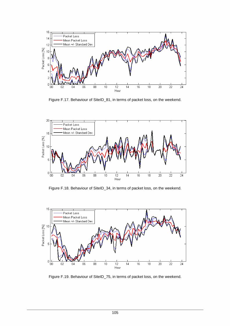
105
Figure F.17. Behaviour of SiteID_81, in terms of packet loss, on the weekend.
Figure F.18. Behaviour of SiteID_34, in terms of packet loss, on the weekend.
Figure F.19. Behaviour of SiteID_75, in terms of packet loss, on the weekend.
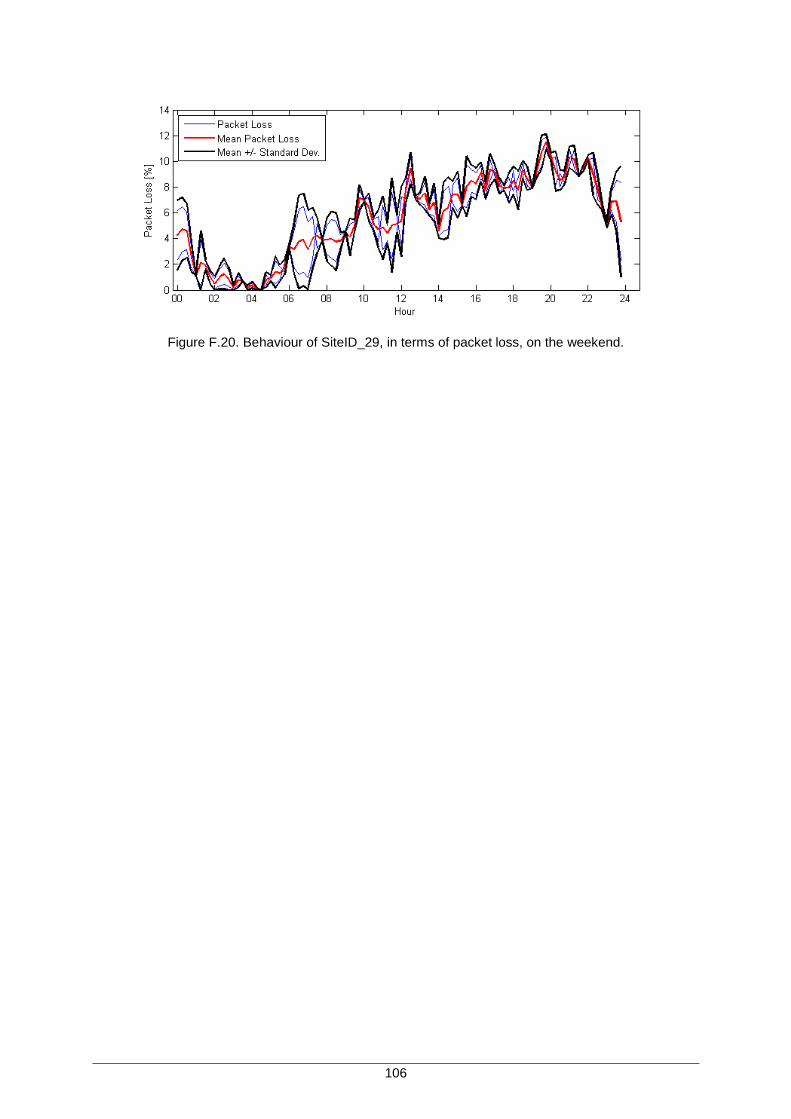
106
Figure F.20. Behaviour of SiteID_29, in terms of packet loss, on the weekend.
107
Annex G
UMTS Network Performance
Maps
G Annex G - UMTS Network Performance Maps
(Confidential)
This annex contains the performance maps resulting from the analysis of the described UMTS
scenario with the developed program.

108
109
Annex H
LTE Network Performance
Maps
H Annex H - LTE Network Performance Maps
(Confidential)
This annex contains the performance maps resulting from the analysis of the described LTE scenario
with the developed program.

110
111
References
References
[3GPP13] http://www.3gpp.org/lte-advanced, Oct. 2013.
[3GPP13a] 3GPP, LTE; Evolved Universal Terrestrial Radio Access (E-UTRA); LTE physical layer;
General description, ETSI TS, No. 136 201, Ver. 11.1.0, Fev. 2013 (http://www.etsi.org/
deliver/etsi_ts/136200_136299/136201/11.01.00_60/ts_136201v110100p.pdf).
[3GPP13b] 3GPP, Digital cellular telecommunications system (Phase 2+); Universal Mobile
Telecommunications System (UMTS); LTE; Policy and charging control architecture,
ETSI TS, No. 123 203, Ver. 11.11.0, Sep. 2013 (http://www.etsi.org/deliver/
etsi_ts/123200_123299/123203/11.11.00_60/ts_123203v111100p.pdf).
[3GPP13c] 3GPP, Evolved Universal Terrestrial Radio Access (E-UTRA); User Equipment (UE) radio
transmission and reception, ETSI TS, No. 136.101, Ver. 11.6.0, Oct. 2013
(http://www.etsi.org/deliver/etsi_ts/136100_136199/136101/11.06.00_60/ts_136101v1106
00p.pdf).
[4GAm11] 4G Americas, Coexistence of GSM, HSPA and LTE, May 2011 (http://
www.4gamericas.org/documents/4G_Americas_Coexistence_of_GSM_HSPA_LTE_May
2011x.pdf).
[ArFi10] Arlos,P., Fiedler,M., “Influence of the Packet Size on the One-Way Delay on the Down-
link in 3G Networks”, in Proc. 5th International Symposium on Wireless Pervasive
Computing (ISWPC), Modena, Italy, May 2010 (http://ieeexplore.ieee.org/stamp/
stamp.jsp?tp=&arnumber=5483732)
[ANAC11] ANACOM, Multiband Auction (in Portuguese), Oct. 2011 (http://www.anacom.pt/
render.jsp?categoryId=340922).
[AlLu11] Alcatel-Lucent, LTE Evolved Packet System Architecture, 2011 (http://lte.alcatel-
lucent.com/locale/en_us/downloads/LTE_poster.pdf).
[Cart13] Cartaxo,A., Optical Fibre Telecommunications Systems – Lecture Notes, Instituto
Superior Técnico, Lisbon, Portugal, 2013.
[Cisc13] Cisco VNI Forecast, Cisco Visual Networking Index Global Mobile Data Traffic Forecast
Update, 2012–2017, Feb. 2013 (http://www.cisco.com/en/US/solutions/collateral/ns341/
ns525/ns537/ns705/ns827/white_paper_c11-520862.pdf).
[Corr13] Correia,L.M., Mobile Communication Systems – Lecture Notes, Instituto Superior
Técnico, Lisbon, Portugal, 2013.
112
[DaPS11] Dahlman,E., Parkvall,S., Sköld,J., 4G LTE/LTE-Advanced for Mobile Broadband,
Elsevier, Oxford, United Kingdom, 2011.
[Ekst09] Ekstrom,H., QoS Control in the 3GPP Evolved Packet System, IEEE Communications
Magazine, Feb. 2009 (http://ieeexplore.ieee.org/stamp/stamp.jsp?arnumber=04785383).
[Eric12] Ericsson Technical Report, IP PROBE SYSTEM, Stockholm, Sweden, Oct. 2012.
[Eric13] Ericsson White Paper, LTE Release 12, Stockholm, Sweden, Jan. 2013
(http://www.ericsson.com/res/docs/ whitepapers/wp-lte-release-12.pdf).
[Eric13a] Ericsson Technical Design Specification, MBH 13B – PM Solution, Stockholm, Sweden
Jun. 2013.
[Eric13b] Ericsson Technical Report, HLD LTE 20120606, Stockholm, Sweden, Jun. 2012
[Eric13c] Ericsson, Performance Management Guidelines – Operating Guidelines, Stockholm,
Sweden, Apr. 2013.
[Eric13d] Ericsson Technical Design Specification, MBH 13B – OAM Solution, Stockholm, Sweden,
Jun. 2013.
[ESAT] Ericsson Stats Analysis Tool v1.1.9, Stockholm, Sweden, 2013.
[EvSk10] Everitt,B.S., Skrondal,A., The Cambridge Dictionary of Statistics, Cambridge University
Press, Cambridge, United Kingdom, 2010.
[Flor09] Flore,D., LTE RAN Architecture aspects, 3GPP Workshop, Beijing, China, Dec. 2009
(http://www.3gpp.org/ftp/workshop/2009-12-17_ITU-R_IMT-Adv_eval/docs/pdf/REV-
090005%20LTE%20RAN%20Architecture%20aspects.pdf).
[HoTo07] Holma,H., Toskala,A., WCDMA for UMTS – HSPA Evolution and LTE, Wiley,
Chippenham, United Kingdom, 2007.
[HoTo09] Holma,H., Toskala,A., LTE for UMTS – OFDMA and SC-FDMA Based Radio Access,
Wiley, Chippenham, United Kingdom, 2009.
[ITUT08] ITU-T, OAM functions and mechanisms for Ethernet based networks, Y.1731, Feb. 2008.
[LSRM12] Laner,M., Svoboda,P., Romirer-Maierhofer,P., Nikaein,N., Ricciato,F., Rupp,M., “A
Comparison Between One-way Delays in Operating HSPA and LTE Networks”, in Proc.
of 8th International Workshop on Wireless Network Measurements, Paderborn, Germany,
May 2012 (http://ieeexplore.ieee.org/stamp/stamp.jsp?tp=&arnumber=6260469).
[Mart12] Martins,A., Evaluation of data applications quality service over UMTS, M.Sc. Thesis,
IST/TUL, Lisbon, Portugal, 2012.
[MatL14] MATLAB Documentation Centre, May 2014 (http://www.mathworks.com/help/stats/
continuous-distributions.html)
[Moto09] Motorola, UMTS/HSPA to LTE Migration – Maximize the life and value of existing assets
while achieving a true 4G network, 2009 (http://www.motorolasolutions.com/web/
113
Business/_Documents/static%20files/UMTS_to_LTE_Migration_White_Paper.pdf).
[PHJI07] Prokkola,J., Hanski,M., Jurvansuu,M., Immonen,M., “Measuring WCDMA and HSDPA
Delay Characteristics with QoSMeT”, in IEEE International Conference on
Communications 2007 (ICC-2007), Glasgow, UK, Jun. 2007
(http://ieeexplore.ieee.org/stamp/stamp.jsp?tp=&arnumber=4288758).
[RomJ04] Romeu, J., “The Chi-Square: a Large-Sample Goodness of Fit Test”, START – Selected
Topics in Assurance Related Technologies, Vol. 10, No. 4, 2004
[RumH08] Rumney,H., 3GPP LTE: Introducing Single-Carrier FDMA, Agilent Technologies Inc.,
U.S.A., Jan. 2008 (http://cp.literature.agilent.com/litweb/pdf/5989-7898EN.pdf).
[Sale02] Salema,C., Feixes Hertzianos, IST Press, Lisbon, Portugal, 2002.
[SeTB11] Sesia,S., Toufik,I., Baker,M., LTE – The UMTS Long Term Evolution, Wiley, Chichester,
United Kingdom, 2011.