M A T H E M A T I C A L E C O N O M I C S

No. 7(14) 2011

Agnieszka Stanimir

Department of Econometrics, Wrocław University of Economics, Komandorska Street 118/120,

53-345 Wrocław, Poland.

E-mail: agnieszka.stanimir@ue.wroc.pl

ANALYSIS OF NOMINAL DATA

– MULTI-WAY CONTINGENCY TABLE

Agnieszka Stanimir

Abstract. Presented in this paper the method of graphical presentation of the relationship

between nominal variables and their categories gives the opportunity for an extensive

diagnosis of dependence variables. Correspondence analysis and mosaic plots are based on

the same grounds, i.e. contingency table or multi-way contingency table. Correspondence

analysis can be used in the study of relationships between two or more nominal variables

without limiting the number of categories. In the case of many variables, the multi-

dimensional contingency table is used very often. Only the difficulty of construction of

such a table and the combined variables can affect the decision of a researcher about the

validity of using this solution. For mosaic plots the situation is different. These graphs

represent very well the relationships between two categories of nominal variables with few

categories. The introduction of another variable to the study, which is described by two or

three categories, is also not too problematic, and the graph is easy to interpret. However, if

in a multi-way contingency table variables are a combination of several primary variables,

described with many categories, the mosaic plot is no longer as clear as the projection made

in correspondence analysis.

Keywords: nominal data, multi-way contingency table, mosaic display, correspondence

analysis.

JEL Classification: C38, J21.

1. Introduction

The aim of this article is the presentation and popularization of mosaic

displays. These charts are a method of analysis and graphical presentation of

nominal variables. Mosaic displays therefore are an alternative to corre-

spondence analysis. The basic approaches of both indicated methods are

based on frequencies of two nominal variables from the contingency table.

In each cell of this table one can observe the frequency of two categories

from two different variables. There is no restriction on the maximum num-

Agnieszka Stanimir

230

ber of categories of variables. In the literature, there is only a limitation on

the number of cells, up to 5, given by Yule, Kendall (1966, p. 471); Blalock

(1975, p. 250). Mosaic graphs do not require the use of reduction of dimen-

sionality methods, such as correspondence analysis.9 This paper shows the

way of conducting both methods for many variables. If the analyzed vari-

ables are more than two, the plotting in a mosaic way is possible after sav-

ing the variables in a multidimensional contingency table. Correspondence

analysis gives many more opportunities, for example, it is possible to ana-

lyse data from the Burt matrix or the concatenated contingency table. How-

ever, to compare the results of both methods, correspondence analysis was

also conducted for multidimensional contingency table.

To illustrate the procedure in both methods, we used the data from the

statistical yearbook of Labour Force Survey. II quarter 2011 (Aktywność

ekonomiczna...). The variables, their categories and the number of occur-

rences are discussed in Section 5.

2. Multiway contingency table

To present the construction of a multidimensional contingency table, it

is necessary to introduce the basic terms of contingency tables for the two

variables.

Let us assume that the number of categories in variable A is r and

in variable B – c, then the nij is the observed frequency10

of category i of

variable A (i = 1, ..., r) and of category j of variable B (j = 1, ..., c). For

Pearson χ2

test of independence should be determined successively: row

sums (row frequencies) in ni ijj

c

1

; column sums (row frequencies)

jn nj iji

r

1

. Row and column sums gives information about the total count

of categories of both variables. Next there are observed proportion ,ij

ij

np

n

which is the percentage share of occurrence in the study of category i of

9 The way to create a mosaic charts for data from contingency table is described in

detail in my work: “Visualization of nominal variables – correspondence analysis and

graphs mosaic” (2011, in press). 10

The terminology used to describe the components of the contingency table is different

among authors, but that used in this work was taken from Goodman (1963); Greenacre

(1993); Jobson (1992).

Analysis of nominal data – multi-way contingency table

231

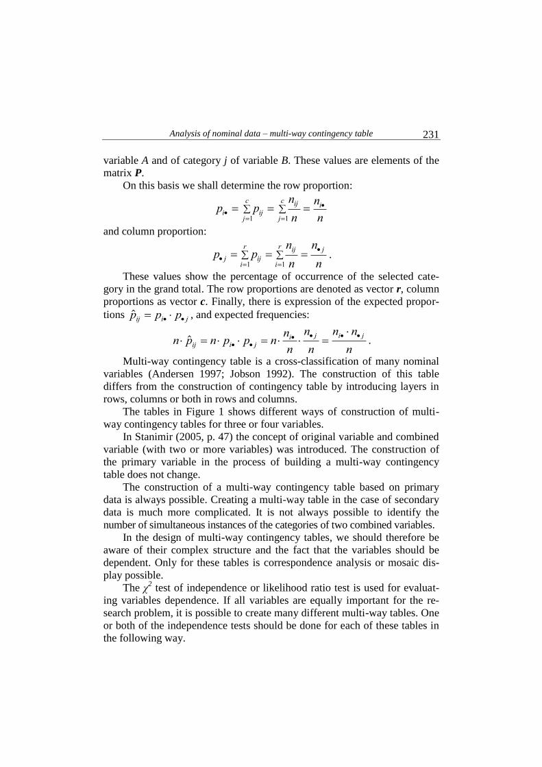
variable A and of category j of variable B. These values are elements of the

matrix P.

On this basis we shall determine the row proportion:

p pn

n

n

ni ij

j

c ij

j

ci

1 1

and column proportion:

p pn

n

n

nj ij

i

r ij

i

r j

1 1

.

These values show the percentage of occurrence of the selected cate-

gory in the grand total. The row proportions are denoted as vector r, column

proportions as vector c. Finally, there is expression of the expected propor-

tions p p pij i j , and expected frequencies:

n p n p p nn

n

n

n

n n

nij i j

i j i j

.

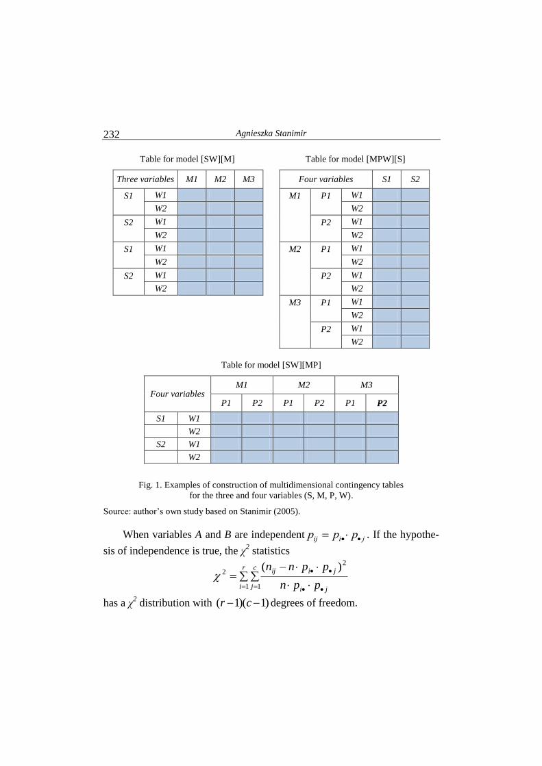
Multi-way contingency table is a cross-classification of many nominal

variables (Andersen 1997; Jobson 1992). The construction of this table

differs from the construction of contingency table by introducing layers in

rows, columns or both in rows and columns.

The tables in Figure 1 shows different ways of construction of multi-

way contingency tables for three or four variables.

In Stanimir (2005, p. 47) the concept of original variable and combined

variable (with two or more variables) was introduced. The construction of

the primary variable in the process of building a multi-way contingency

table does not change.

The construction of a multi-way contingency table based on primary

data is always possible. Creating a multi-way table in the case of secondary

data is much more complicated. It is not always possible to identify the

number of simultaneous instances of the categories of two combined variables.

In the design of multi-way contingency tables, we should therefore be

aware of their complex structure and the fact that the variables should be

dependent. Only for these tables is correspondence analysis or mosaic dis-

play possible.

The χ2 test of independence or likelihood ratio test is used for evaluat-

ing variables dependence. If all variables are equally important for the re-

search problem, it is possible to create many different multi-way tables. One

or both of the independence tests should be done for each of these tables in

the following way.

Agnieszka Stanimir

232

Table for model [SW][M] Table for model [MPW][S]

Three variables M1 M2 M3 Four variables S1 S2

S1 W1 M1 P1 W1

W2 W2

S2 W1 P2 W1

W2 W2

S1 W1 M2 P1 W1

W2 W2

S2 W1 P2 W1

W2 W2

M3 P1 W1

W2

P2 W1

W2

Table for model [SW][MP]

Four variables M1 M2 M3

P1 P2 P1 P2 P1 P2

S1 W1

W2

S2 W1

W2

Fig. 1. Examples of construction of multidimensional contingency tables

for the three and four variables (S, M, P, W).

Source: author‟s own study based on Stanimir (2005).

When variables A and B are independent pij p pi j . If the hypothe-

sis of independence is true, the χ2 statistics

r

i

c

j ji

jiij

ppn

ppnn

1 1

2

2)(

has a χ2 distribution with )1)(1( cr degrees of freedom.

Analysis of nominal data – multi-way contingency table

233

In the Likelihood ratio approach the statistics

L nn

nij

ij

ijj

c

i

r2

11

2

ln

,

where nij are expected frequencies; L2 “has a χ

2 distribution with )1)(1( cr

degrees of freedom if the hypothesis of independence is held” (Jobson, 1992,

p. 21).

Clausen (1998) and van der Heijden (1987) suggest that further analysis

is performed for an array with higher dependences between variables.

3. Mosaic displays

Mosaic displays are a modification of sieve and parquet diagrams. The

largest contribution to the dissemination of this type of analysis was made

by Fiendly (for example 1992, 1994).

A mosaic (sieve) plot is composed of rectangles. In English-language

literature there are many terms used for rectangles such as bin, box, tiles

(see (Hofmann, 2000; Friendly, 1992)). As a basis of mosaic charts, we can

use cumulative bar charts. Each bar is divided vertically, depending on the

frequencies of categories of the second variable.

In the case of contingency table analysis, the area of each plate on sieve

diagram is proportional to the cell expected frequency. However, the ob-

served frequencies are shown by the number of squares in each rectangle.

The difference between the observed and expected cell frequencies is shown

by line shading or colours. Positive deviations are presented in one colour or

solid lines, negative – a different colour or a dotted line.

On the mosaic plot, each cell of contingency table is presented as

a plate whose area corresponds to the cell frequency in the table cell. The

width of each rectangle is proportional to column frequencies and the height

is proportional to the conditional frequency of each row |

•

ij

i j

j

nn

n . This

method of mosaic plot construction was proposed by Friendly (1994). In

Friendly‟s graphs the heights of tiles for row categories are different in

correspondence to the following column categories. In Friendly‟s plots it is

easy to observe the independence of variables because in the case of com-

plete independence the height of tiles in each row will be the same.

Agnieszka Stanimir

234

Another modification proposed by Friendly (1994) in comparison to

sieve diagrams is the use of shading and reordering of corresponding cate-

gories (both in rows and in columns). The plot becomes more clear and

consistent. Friendly (1994) proposes that the colours and shadings should

correspond to the standardized deviations from independence, which are

calculated as ˆ

ˆ

ij iijj

ij

iijj

n npm

np

. The shading for a cell with positive devia-

tions is drawn with black solid lines from upper left to the lower right corner

of the tile. When 0ijm shading is done with a red, broken line from upper

right to the lower left corner, the absolute value of deviations is presented in

the density of lines placed on the plate. “Cells with absolute values less than

2 are empty and cells with 2ijm are filled, those with 4ijm are filled

with a darker pattern” (Friendly, 1994, p. 191).

In the use of mosaic plots for analyzing data from multi-way contin-

gency table, every tile will be divided. Suppose that the analysis concerns

three variables (A, B, W). If the combined variable is defined as [AB], so the

analyzed table will be [AB] [W]. In this case, each rectangle corresponding

to the categories of variable A will be divided into smaller rectangles whose

number is consistent with the number of categories of variable B.

4. Correspondence analysis

Correspondence analysis is a method to study associations between

categories of nominal variables. But on the measurement scales, it is possi-

ble to transform values from stronger to weaker scales (Walesiak, 1996).

Therefore, a correspondence analysis may be conducted for variables meas-

ured on the stronger scales after the transformation. Correspondence analy-

sis belongs to a group of methods based on the reduction of dimensionality.

In the classical correspondence analysis approach the relationships of cate-

gories of two nominal variables are examined. Taking indications of Section 2,

the full dimensional space is min{r – 1; c – 1}. So if each of the nominal

variables is described by more than four categories, the graphical presenta-

tion of the relationships between them is not possible. Therefore, the singu-

lar value decomposition is used and on that basis the best space of presenta-

tion of results is chosen. A detailed description of the procedure in the cor-

respondence analysis can be found in Stanimir (2005).

Analysis of nominal data – multi-way contingency table

235

The result of correspondence analysis is presented as a scatter of points

showing the categories of the analyzed variables. If the categories derived

from two different variables are close together, it means that their co-

occurrence is frequent. Points located farthest from the centre of gravity

have the most influence on the variable dependences, as opposed to the

points located near the centre.

Correspondence analysis of the data from a multi-way contingency ta-

ble is performed as a classical contingency table analysis. However, note

that the each combined variable should be treated as a consistent variable.

Consequently, for example, if the analyzed table is constructed as follows:

[AB] [W], so its categories are as follows a1b1, a1b2,…, a1bj, a2b1, a2b2, …

a2bj, …, aib1, aib2, …, aibj. Categories of a combined variable created in that

way cannot be shared during the interpretation of the results, which means

that the position of the point cannot be interpreted to indicate the category a2

without any of the categories of variable B.

5. Example of the use of mosaic display and correspondence analysis

in the study of economic activity

The statistical yearbook of Labour Force Survey. II quarter 2011

(Aktywność ekonomiczna…, 2011) contains data to analyze the problem of

economic activity, taking into account many factors. In the conducted study,

the author decided to see how the economic activity of the Polish population

by gender and education differs. To achieve the research goal, it was neces-

sary to select the following variables:

economic activity: full-time employed persons (A1), part-time em-

ployed persons (A2), unemployed persons (A3), persons economically

inactive (A4);

level of education: tertiary (E1), post-secondary (E2), vocational

secondary (E3), general secondary (E4), basic vocational (E5), lower secon-

dary, primary and incomplete primary (E6);

gender: females (G1), males (M2).

Labour Force in Poland in II quarter 2011 is presented in Table 1.

The analysis of the data from Table 1 with mosaic graphs, has bene-

fited from the software Mosaic Displays proposed by Friendly on web page:

http://euclid.psych.yorku.ca/cgi/mosaics.

Fillings available in Friendly‟s software are slightly different from

those described earlier. Tiles shading presented in Section 3 is carried out

with lines. In Friendly‟s software squares are used like in sieve diagrams.

Agnieszka Stanimir

236

Table 1. Economic activity in Poland (II quarter 2011, in thousands): females and males

Economic activity: females

A1 A2 A3 A4

Ed

uca

tio

nal

lev

el

E1 2 388 192 159 752

E2 356 36 44 248

E3 1 525 166 171 1 327

E4 652 111 126 1 230

E5 1 205 179 211 1 495

E6 333 111 103 3 569

Economic activity: males

A1 A2 A3 A4

Ed

uca

tio

nal

lev

el

E1 1 842 96 88 397

E2 181 7 20 50

E3 2 216 94 174 782

E4 581 42 83 478

E5 2 984 138 345 1 379

E6 616 112 166 2 294

Source: author‟s own study based on Aktywność ekonimiczna... (2011).

Tiles with positive deviations are drawn with blue colour, with red –

negative deviations. If 2ijm , the tiles are not filled, when 2ijm are

filled with squares, those with 4ijm are filled with dense squares.

For a given variable it was possible to build three multi-way contin-

gency tables: [EG][A], [AG][E], [AE][G]. However, one third of these

tables would contain two columns, and thus the presentation of the results of

correspondence analysis would be in R1 space. The research problem also

tends to use this table where the educational level and gender are combined

into one variable.

5.1. Breakdown of the level of education by gender in association with

economic activity

After creating a new variable, new categories are also created. For cor-

respondence analysis, it is necessary to encode these categories as E1G1

(women with tertiary education), E1G2 (men with tertiary education), E2G1

(women with post-secondary education), E2G2 (men with post-secondary

education), …, E6G1 (women with lower secondary, primary or incomplete

primary education), E6G2 (women with lower secondary, primary or in-

complete primary education). Table 2 presents this data.

Analysis of nominal data – multi-way contingency table

237

Table 2. Breakdown of the level of education by gender in association with economic activity

Economic activity

A1 A2 A3 A4

Lev

el o

f ed

uca

tio

n b

y g

end

er E1G1 2 388 192 159 752

E1G2 1 842 96 88 397

E2G1 356 36 44 248

E2G2 181 7 20 50

E3G1 1 525 166 171 1 327

E3G2 2 216 94 174 782

E4G1 652 111 126 1 230

E4G2 581 42 83 478

E5G1 1 205 179 211 1 495

E5G2 2 984 138 345 1 379

E6G1 333 111 103 3 569

E6G2 616 112 166 2 294

Source: author‟s own study based on Aktywność ekonomiczna... (2011).

For this data, the χ2 statistics and likelihood ratio L2 are respectively

7426.6 and 7970.16 on 33 df, indicating the high dependence between

variables.

E1G2

E4G1E4G2

E5G1

E5G2

E6G1

E6G2

A1A2A3

A4

-0,8 -0,6 -0,4 -0,2 0,0 0,2 0,4 0,6 0,8 1,0 1,2

l1=0.23 (96.82% of total inertia)

-0,8

-0,6

-0,4

-0,2

0,0

0,2

0,4

0,6

0,8

1,0

1,2

l 2=

0.0

04

(1

.88

% o

f to

tal

iner

tia)

E1G2

E4G1E4G2

E5G1

E5G2

E6G1

E6G2

A1A2A3

A4E2G2 E3G1E1G1

E3G2

E2G1

Fig. 2. Correspondence analysis of economic activity and level

of education broken down by gender

Source: own study based on Aktywność ekonomiczna... (2011).

Agnieszka Stanimir

238

Fig. 3. Mosaic display of economic activity and level of education broken down by gender

Source: author‟s own study based on Aktywność ekonomiczna... (2011).

Analysis of nominal data – multi-way contingency table

239

6. Summary

Methods of graphical presentation of the relationship between nominal

variables and their categories described in this paper gave the opportunity

for an extensive diagnosis of dependence variables. Correspondence analy-

sis and mosaic plots are based on the same grounds, i.e. contingency table or

multi-way contingency table.

Correspondence analysis can be used in the study of relationships be-

tween two or more nominal variables without limiting the number of catego-

ries. In the case of many variables, very often the multi-dimensional contin-

gency table is used. Only the difficulty of construction of such a table and

the combined variables can affect the decision of a researcher about the

validity of using this solution.

For mosaic plots the situation is different. These graphs in a very good

way represent the relationships between two categories of nominal variables

with few categories. The introduction of another variable to the study, which

is described by two or three categories is also not too problematic, and the

graph is easy to interpret. However, if in a multi-way contingency table

variables are combined of several of primary variables, described with many

categories, the mosaic plot is no longer as clear as the projection made in the

correspondence analysis.

Literature

Aktywności ekonomiczna ludności Polski. II kwartał 2011 (2011). GUS. Warszawa.

Andersen E.B. (1997). Introduction to the Statistical Analysis of Categorical Data.

Springer-Verlag. Berlin.

Blalock H.M. (1975). Statystyka dla socjologów. PWN. Warszawa.

Clausen S.E. (1998). Applied Correspondence Analysis. An Introduction. Sage.

University Paper 121.

Friendly M. (1992). Mosaic displays for loglinear models. In: Proceedings of the

Statistical Graphic Section. Pp. 61-68.

Friendly M. (1994). Mosaic display for multi-way contingency tables. Journal of

the American Statistical Association. Vol. 89. No. 425. Pp. 190-200.

Goodman L.A. (1963). On Plackett’s test for contingency table interactions. Jour-

nal of the Royal Statistical Society. Series B. Vol. 25. No. 1. Pp. 179-188.

Greenacre M. (1993). Correspondence Analysis in Practice. Academic Press.

London.

Heijden van der, P.G.M. (1987). Correspondence Analysis of Logitudinal Catego-

rical Data. DSWO Press. Leiden.

Agnieszka Stanimir

240

Jobson J.D. (1992). Applied Multivariate Data Analysis. Vol. II. Categorical and

Multivariate Methods. Springer-Verlag. New York.

Hofmann H. (2000). Exploring categorical data: Interactive mosaic plots. Metrika.

Vol. 51. Pp. 11-26.

Stanimir A. (2005). Analiza korespondencji jako narzędzie do badania zjawisk

ekonomicznych. Wydawnictwo Akademii Ekonomicznej. Wrocław.

Walesiak M. (1996). Metody analizy danych marketingowych. PWN. Warszawa.

Yule G.U, Kendall M.G. (1966). Wstęp do teorii statystyki. PWN. Warszawa.