Analysis of nonlinear structural dynamics and resonance in ...downloads.hindawi.com/journals/sv/2012/702712.pdf · 610 H.D. Ganji et al. / Analysis of nonlinear structural dynamics

Shock and Vibration 19 (2012) 609–617 609DOI 10.3233/SAV-2011-0654IOS Press

Analysis of nonlinear structural dynamics andresonance in trees

H. Doumiri Ganjia,∗, S.S. Ganjia,∗, D.D. Ganjib and F. VaseghicaYoung Researchers Club, Science and Research Branch, Islamic Azad University, Tehran, IranbDepartment of Mechanical Engineering, Babol University of Technology, Babol, IrancDepartment of Industerial Engineering, Iran University of Science and Technology, Tehran, Iran

Received 23 January 2011

Revised 17 August 2011

Abstract. Wind and gravity both impact trees in storms, but wind loads greatly exceed gravity loads in most situations. Complexbehavior of trees in windstorms is gradually turning into a controversial concern among ecological engineers. To better understandthe effects of nonlinear behavior of trees, the dynamic forces on tree structures during periods of high winds have been examinedas a mass-spring system. In fact, the simulated dynamic forces created by strong winds are studied in order to determine theresponses of the trees to such dynamic loads. Many of such nonlinear differential equations are complicated to solve. Therefore,this paper focuses on an accurate and simple solution, Differential Transformation Method (DTM), to solve the derived equation.In this regard, the concept of differential transformation is briefly introduced. The approximate solution to this equation iscalculated in the form of a series with easily computable terms. Then, the method has been employed to achieve an acceptablesolution to the presented nonlinear differential equation. To verify the accuracy of the proposed method, the obtained results fromDTM are compared with those from the numerical solution. The results reveal that this method gives successive approximationsof high accuracy solution.

Keywords: Tree, mass-spring system, oscillation, runge–kutta method, analytical solution

1. Introduction

Wind damage has always been a global phenomenon that affects tropical, temperate and plantation forests [1],such as Hurricane Hugo in South Carolina [2] and Storm Vivian in Northern Europe [3]. Such storms severely affectforest management. Wind loads are the largest dynamic loads on trees [4]. Loads caused by wind are periodic andcreate a sway motion in trees which can be simplified using a conceptual model of a tree stem [5] without branchesand being considered as an upside-down pendulum [6]. Recently, there have been a variety of models consideringresonance behavior in plant stems [7]. A number of mathematical models such as mass-spring–damper systems havebeen proposed to anticipate stem dynamics and natural frequencies [8].

In most cases, such problems do not admit analytical solution, so these equations have to be solved using specialtechniques. In recent years, much attention has been devoted to the newly developed methods to construct ananalytic solution to these equations, including the Perturbation techniques. Perturbation techniques are too stronglydependent upon the so-called “small parameters” [9]. Many other methods have been introduced to solve nonlinearequations such as homotopy perturbation [10–13] and analysis methods [14,15], variational approach [16,17],parameter expanding [18,28], Max-Min Approach [MMA] [19], and Amplitude–Frequency Formulation (AFF) [20,27]. One of the semi-exact methods which do not need linearization is differential transform method (DTM) whichhas attracted many authors to use this method for solving nonlinear oscillator dynamic problems [21–23].

∗Corresponding authors. E-mail: [email protected]; [email protected].

ISSN 1070-9622/12/$27.50 2012 – IOS Press and the authors. All rights reserved

610 H.D. Ganji et al. / Analysis of nonlinear structural dynamics and resonance in trees

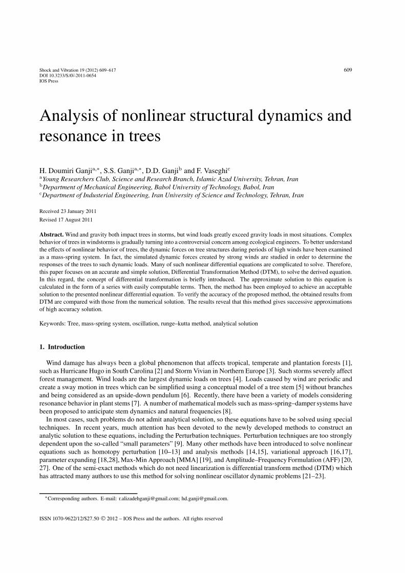
Fig. 1. Dynamic model of a tree trunk (structure) represented as a mass (m) oscillating on a spring (k) with the motion being damped (d).

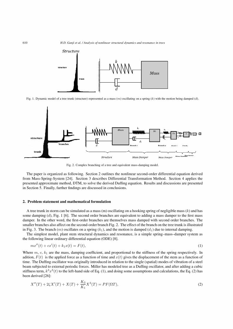
Fig. 2. Complex branching of a tree and equivalent mass-damping model.

The paper is organized as following. Section 2 outlines the nonlinear second-order differential equation derivedfrom Mass-Spring-System [24]. Section 3 describes Differential Transformation Method. Section 4 applies thepresented approximate method, DTM, to solve the derived Duffing equation. Results and discussions are presentedin Section 5. Finally, further findings are discussed in conclusions.

2. Problem statement and mathematical formulation

A tree trunk in storm can be simulated as a mass (m) oscillating on a hooking spring of negligible mass (k) and hassome damping (d), Fig. 1 [6]. The second order branches are equivalent to adding a mass damper to the first massdamper. In the other word, the first-order branches are themselves mass damped with second order branches. Thesmaller branches also affect on the second-order branch Fig. 2. The effect of the branch on the tree trunk is illustratedin Fig. 3. The branch (m) oscillates on a spring (k1), and the motion is damped (d1) due to internal damping.

The simplest model, plant stem structural dynamics and resonance, is a simple spring–mass–damper system asthe following linear ordinary differential equation (ODE) [8].

mx′′(t) + cx′(t) + k1x(t) = F (t), (1)

Where m, c, k1 are the mass, damping coefficient, and proportional to the stiffness of the spring respectively. Inadition, F (t) is the applied force as a function of time and x(t) gives the displacement of the stem as a function oftime. The Duffing oscillator was originally introduced in relation to the single (spatial) modes of vibration of a steelbeam subjected to external periodic forces. Miller has modeled tree as a Duffing oscillator, and after adding a cubicstiffness term, k3x3(t) to the left-hand side of Eq. (1), and doing some assumptions and calculations, the Eq. (2) hasbeen derived [26]:

X ′′(T ) + 2ζX ′(T ) + X(T ) +K3

K1X3(T ) = PF (ΩT ), (2)

H.D. Ganji et al. / Analysis of nonlinear structural dynamics and resonance in trees 611

Fig. 3. Dynamic model of a trunk with branch (mass damper) attached.

K1 = k1Lmax, K3 = k3(Lmax)3, P =p0

K1, Ω =

ω

ω0, X =

x

Lmax, T = ω0 t, .

Where k3 is the stiffness coefficient. Lmax is a characteristic maximumdeflection. In this case, Lmax is the deflectionat which failure occurs with well known oscillator boundary conditions as follows

X(0) = 1, X ′(0) = 0. (3)

Where K3/K1 and p0/K1 will be referred to as the nonlinear ratio and the normalized forcing amplitude, respectively.The forcing term could be set to the following:

F (ΩT ) =12

(1 + sin (ΩT )) . (4)

3. Fundamentals of differential transformation method

We suppose x(t) to be analytic function in a domain D and t = ti represent any point in D. The function x(t) isthen represented by one power series whose center is located at ti. The Taylor series expansion function of x(t) isof the form [25,26].

x(t) =∞∑

k=0

(t − ti)k

k!

[dkx(t)

dtk

]t=ti

∀t ∈ D, (5)

When ti = 0 is referred to as the Maclaurin series of x(t) and is expressed as:

x(t) =∞∑

k=0

tk

k!

[dkx(t)

dtk

]t=0

∀t ∈ D, (6)

The differential transformation of the function x(t) is defined as follows:

X(k) =∞∑

k=0

Hk

k!

[dkx(t)

dtk

]t=0

, (7)

Where x(t) the original is function and X(k) is the transformed function. The differential spectrum of X(k) isconfined within the interval t ∈ [0, H ], where H is a constant. The differential inverse transform of X(k) is definedas follows:

x(t) =∞∑

k=0

(t

H

)k

X(k), (8)

It is clear that the concept of differential transformation is based upon the Taylor series expansion. The values offunction X(k) at t values of argument k are referred to as discrete, i.e. X(0) is known as the zero discrete, X(1) asthe first discrete, etc. The more discrete available, the more precisely it is possible to restore the unknown function.The function x(t) consists of the T-function X(k), and its value is given by the sum of the T-function with (t/H)k


Table 1The fundamental operations of differential transform method

Original function Transformed function

x(t) = αf(x) ± βg(t) X(k) = αF (k) ± βG(k)

x(t) =df(t)

dtX(k) = (k + 1)F (k + 1)

x(t) =d2f(t)

dt2X(k) = (k + 1)(k + 2)F (k + 2)

x(t) = exp(t) X(k) = kk!

x(t) = f(t)g(t) X(k) =k∑

l=0

F (l)G(k − l)

x(t) = tm X(k) = δ(k − m) =

{1 k = m0 k �= m

x(t) = sin(ω t + α) X(k) = ωk

k!sin

(πk2

+ α)

x(t) = cos(ω t + α) X(k) = ωk

k!cos

(πk2

+ α)

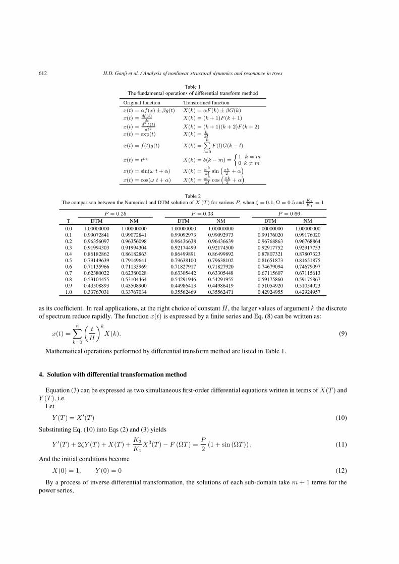
Table 2The comparison between the Numerical and DTM solution of X (T ) for various P , when ζ = 0.1, Ω = 0.5 and K3

K1= 1

P = 0.25 P = 0.33 P = 0.66

T DTM NM DTM NM DTM NM

0.0 1.00000000 1.00000000 1.00000000 1.00000000 1.00000000 1.000000000.1 0.99072841 0.99072841 0.99092973 0.99092973 0.99176020 0.991760200.2 0.96356097 0.96356098 0.96436638 0.96436639 0.96768863 0.967688640.3 0.91994303 0.91994304 0.92174499 0.92174500 0.92917752 0.929177530.4 0.86182862 0.86182863 0.86499891 0.86499892 0.87807321 0.878073230.5 0.79149639 0.79149641 0.79638100 0.79638102 0.81651873 0.816518750.6 0.71135966 0.71135969 0.71827917 0.71827920 0.74679094 0.746790970.7 0.62380022 0.62380028 0.63305442 0.63305448 0.67115607 0.671156130.8 0.53104455 0.53104464 0.54291946 0.54291955 0.59175860 0.591758670.9 0.43508893 0.43508900 0.44986413 0.44986419 0.51054920 0.510549231.0 0.33767031 0.33767034 0.35562469 0.35562471 0.42924955 0.42924957

as its coefficient. In real applications, at the right choice of constant H , the larger values of argument k the discreteof spectrum reduce rapidly. The function x(t) is expressed by a finite series and Eq. (8) can be written as:

x(t) =n∑

k=0

(t

H

)k

X(k). (9)

Mathematical operations performed by differential transform method are listed in Table 1.

4. Solution with differential transformation method

Equation (3) can be expressed as two simultaneous first-order differential equations written in terms of X(T ) andY (T ), i.e.

Let

Y (T ) = X ′(T ) (10)

Substituting Eq. (10) into Eqs (2) and (3) yields

Y ′(T ) + 2ζY (T ) + X(T ) +K3

K1X3(T ) − F (ΩT ) =

P

2(1 + sin (ΩT )) , (11)

And the initial conditions become

X(0) = 1, Y (0) = 0 (12)

By a process of inverse differential transformation, the solutions of each sub-domain take m + 1 terms for thepower series,


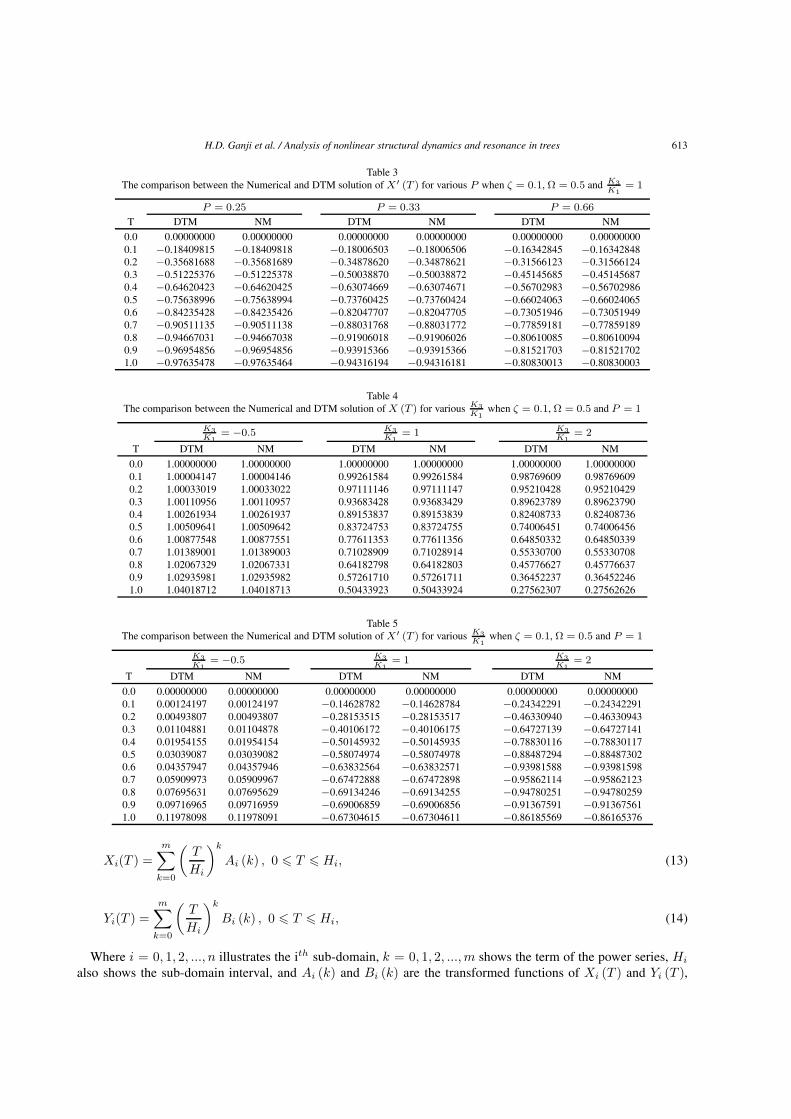
Table 3The comparison between the Numerical and DTM solution of X′ (T ) for various P when ζ = 0.1, Ω = 0.5 and K3

K1= 1

P = 0.25 P = 0.33 P = 0.66


0.0 0.00000000 0.00000000 0.00000000 0.00000000 0.00000000 0.000000000.1 −0.18409815 −0.18409818 −0.18006503 −0.18006506 −0.16342845 −0.163428480.2 −0.35681688 −0.35681689 −0.34878620 −0.34878621 −0.31566123 −0.315661240.3 −0.51225376 −0.51225378 −0.50038870 −0.50038872 −0.45145685 −0.451456870.4 −0.64620423 −0.64620425 −0.63074669 −0.63074671 −0.56702983 −0.567029860.5 −0.75638996 −0.75638994 −0.73760425 −0.73760424 −0.66024063 −0.660240650.6 −0.84235428 −0.84235426 −0.82047707 −0.82047705 −0.73051946 −0.730519490.7 −0.90511135 −0.90511138 −0.88031768 −0.88031772 −0.77859181 −0.778591890.8 −0.94667031 −0.94667038 −0.91906018 −0.91906026 −0.80610085 −0.806100940.9 −0.96954856 −0.96954856 −0.93915366 −0.93915366 −0.81521703 −0.815217021.0 −0.97635478 −0.97635464 −0.94316194 −0.94316181 −0.80830013 −0.80830003

Table 4The comparison between the Numerical and DTM solution of X (T ) for various K3

K1when ζ = 0.1, Ω = 0.5 and P = 1

K3K1

= −0.5 K3K1

= 1 K3K1

= 2


0.0 1.00000000 1.00000000 1.00000000 1.00000000 1.00000000 1.000000000.1 1.00004147 1.00004146 0.99261584 0.99261584 0.98769609 0.987696090.2 1.00033019 1.00033022 0.97111146 0.97111147 0.95210428 0.952104290.3 1.00110956 1.00110957 0.93683428 0.93683429 0.89623789 0.896237900.4 1.00261934 1.00261937 0.89153837 0.89153839 0.82408733 0.824087360.5 1.00509641 1.00509642 0.83724753 0.83724755 0.74006451 0.740064560.6 1.00877548 1.00877551 0.77611353 0.77611356 0.64850332 0.648503390.7 1.01389001 1.01389003 0.71028909 0.71028914 0.55330700 0.553307080.8 1.02067329 1.02067331 0.64182798 0.64182803 0.45776627 0.457766370.9 1.02935981 1.02935982 0.57261710 0.57261711 0.36452237 0.364522461.0 1.04018712 1.04018713 0.50433923 0.50433924 0.27562307 0.27562626

Table 5The comparison between the Numerical and DTM solution of X′ (T ) for various K3

K1when ζ = 0.1, Ω = 0.5 and P = 1

K3K1

= −0.5 K3K1

= 1 K3K1

= 2


0.0 0.00000000 0.00000000 0.00000000 0.00000000 0.00000000 0.000000000.1 0.00124197 0.00124197 −0.14628782 −0.14628784 −0.24342291 −0.243422910.2 0.00493807 0.00493807 −0.28153515 −0.28153517 −0.46330940 −0.463309430.3 0.01104881 0.01104878 −0.40106172 −0.40106175 −0.64727139 −0.647271410.4 0.01954155 0.01954154 −0.50145932 −0.50145935 −0.78830116 −0.788301170.5 0.03039087 0.03039082 −0.58074974 −0.58074978 −0.88487294 −0.884873020.6 0.04357947 0.04357946 −0.63832564 −0.63832571 −0.93981588 −0.939815980.7 0.05909973 0.05909967 −0.67472888 −0.67472898 −0.95862114 −0.958621230.8 0.07695631 0.07695629 −0.69134246 −0.69134255 −0.94780251 −0.947802590.9 0.09716965 0.09716959 −0.69006859 −0.69006856 −0.91367591 −0.913675611.0 0.11978098 0.11978091 −0.67304615 −0.67304611 −0.86185569 −0.86165376

Xi(T ) =m∑

k=0

(T

Hi

)k

Ai (k) , 0 � T � Hi, (13)

Yi(T ) =m∑

k=0

(T

Hi

)k

Bi (k) , 0 � T � Hi, (14)

Where i = 0, 1, 2, ..., n illustrates the ith sub-domain, k = 0, 1, 2, ..., m shows the term of the power series, Hi

also shows the sub-domain interval, and Ai (k) and Bi (k) are the transformed functions of Xi (T ) and Yi (T ),


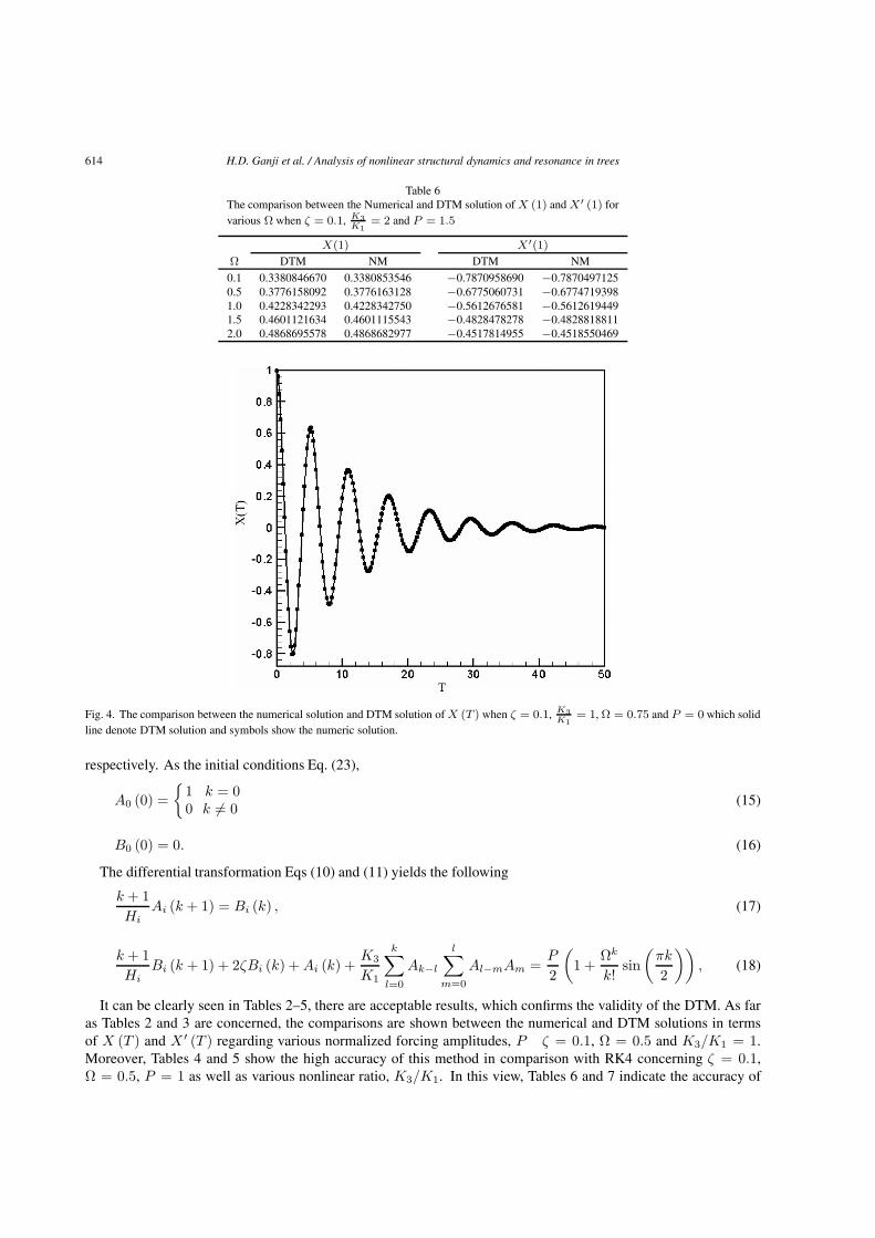
Table 6The comparison between the Numerical and DTM solution of X (1) and X′ (1) forvarious Ω when ζ = 0.1, K3

K1= 2 and P = 1.5

X(1) X′(1)Ω DTM NM DTM NM

0.1 0.3380846670 0.3380853546 −0.7870958690 −0.78704971250.5 0.3776158092 0.3776163128 −0.6775060731 −0.67747193981.0 0.4228342293 0.4228342750 −0.5612676581 −0.56126194491.5 0.4601121634 0.4601115543 −0.4828478278 −0.48288188112.0 0.4868695578 0.4868682977 −0.4517814955 −0.4518550469

Fig. 4. The comparison between the numerical solution and DTM solution of X (T ) when ζ = 0.1, K3K1

= 1, Ω = 0.75 and P = 0 which solidline denote DTM solution and symbols show the numeric solution.

respectively. As the initial conditions Eq. (23),

A0 (0) ={

1 k = 00 k �= 0 (15)

B0 (0) = 0. (16)

The differential transformation Eqs (10) and (11) yields the following

k + 1Hi

Ai (k + 1) = Bi (k) , (17)

k + 1Hi

Bi (k + 1) + 2ζBi (k) + Ai (k) +K3

K1

k∑l=0

Ak−l

l∑m=0

Al−mAm =P

2

(1 +

Ωk

k!sin

(πk

2

)), (18)

It can be clearly seen in Tables 2–5, there are acceptable results, which confirms the validity of the DTM. As faras Tables 2 and 3 are concerned, the comparisons are shown between the numerical and DTM solutions in termsof X (T ) and X ′ (T ) regarding various normalized forcing amplitudes, P ζ = 0.1, Ω = 0.5 and K3/K1 = 1.Moreover, Tables 4 and 5 show the high accuracy of this method in comparison with RK4 concerning ζ = 0.1,Ω = 0.5, P = 1 as well as various nonlinear ratio, K3/K1. In this view, Tables 6 and 7 indicate the accuracy of


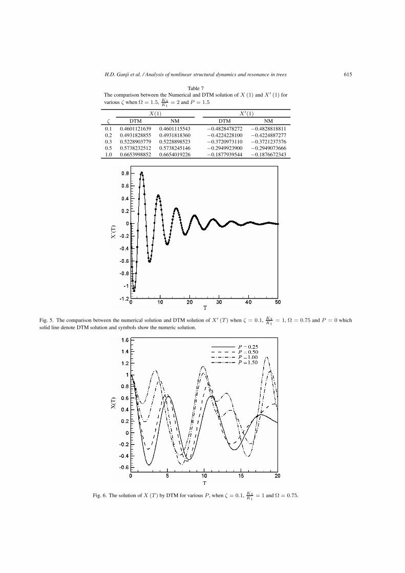
Table 7The comparison between the Numerical and DTM solution of X (1) and X′ (1) forvarious ζ when Ω = 1.5, K3

K1= 2 and P = 1.5

X(1) X′(1)ζ DTM NM DTM NM

0.1 0.4601121639 0.4601115543 −0.4828478272 −0.48288188110.2 0.4931828855 0.4931818360 −0.4224228100 −0.42248872770.3 0.5228903779 0.5228898523 −0.3720973110 −0.37212373760.5 0.5738232512 0.5738245146 −0.2949923900 −0.29490736661.0 0.6653998852 0.6654019226 −0.1877939544 −0.1876672343

Fig. 5. The comparison between the numerical solution and DTM solution of X′ (T ) when ζ = 0.1, K3K1

= 1, Ω = 0.75 and P = 0 whichsolid line denote DTM solution and symbols show the numeric solution.

Fig. 6. The solution of X (T ) by DTM for various P , when ζ = 0.1, K3K1

= 1 and Ω = 0.75.


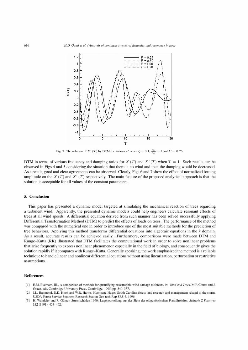
Fig. 7. The solution of X′ (T ) by DTM for various P , when ζ = 0.1, K3K1

= 1 and Ω = 0.75.

DTM in terms of various frequency and damping ratios for X (T ) and X ′ (T ) when T = 1. Such results can beobserved in Figs 4 and 5 considering the situation that there is no wind and then the damping would be decreased.As a result, good and clear agreements can be observed. Clearly, Figs 6 and 7 show the effect of normalized forcingamplitude on the X (T ) and X ′ (T ) respectively. The main feature of the proposed analytical approach is that thesolution is acceptable for all values of the constant parameters.

5. Conclusion

This paper has presented a dynamic model targeted at simulating the mechanical reaction of trees regardinga turbulent wind. Apparently, the presented dynamic models could help engineers calculate resonant effects oftrees at all wind speeds. A differential equation derived from such manner has been solved successfully applyingDifferential Transformation Method (DTM) to predict the effects of loads on trees. The performance of the methodwas compared with the numerical one in order to introduce one of the most suitable methods for the prediction oftree behaviors. Applying this method transforms differential equations into algebraic equations in the k domain.As a result, accurate results can be achieved easily. Furthermore, comparisons were made between DTM andRunge–Kutta (RK) illustrated that DTM facilitates the computational work in order to solve nonlinear problemsthat arise frequently to express nonlinear phenomenon especially in the field of biology, and consequently gives thesolution rapidly if it compares with Runge–Kutta. Generally speaking, the work emphasized the method is a reliabletechnique to handle linear and nonlinear differential equations without using linearization, perturbation or restrictiveassumptions.

References

[1] E.M. Everham, III., A comparison of methods for quantifying catastrophic wind damage to forests, in: Wind and Trees, M.P. Coutts and J.Grace, eds, Cambridge University Press, Cambridge, 1995, pp. 340–357.

[2] J.L. Haymond, D.D. Hook and W.R. Harms, Hurricane Hugo: South Carolina forest land research and management related to the storm.USDA Forest Service Southern Research Station Gen tech Rep SRS-5, 1996.

[3] H. Wandeler and R. Gunter, Sturmschaden 1990: Lagebeurteilung aus der Sicht der eidgenossischen Forstdirektion, Schweiz Z Forstwes142 (1991), 453–462.


[4] C. Mattheck and H. Breloer, The Body Language Of Trees. HMSO, London, UK, 1994.[5] C.J. Wood, Understanding wind forces on trees, 133–164. in: Wind and Trees. Cambridge University Press, M.P. Coutts and J. Grace, eds,

Cambridge, UK, 1995.[6] K. James, Dynamic loading of trees, Journal of Arboriculture 29(3) (2003), 165–171.[7] J.J. Finnigan, Turbulence in plant canopies, Annu Rev Fluid Mech 32 (2000), 519–571.[8] M. Denny, B. Gaylord, B. Helmuth and T. Daniel, The menace of momentum: dynamic forces on flexible organisms, Limnol Oceanogr 43

1998, 955–968.[9] A.H. Nayfeh, Perturbation Methods, Wiley, New York, 2000.

[10] D.D. Ganji and A. Sadighi, Application of He’s Homotopy-perturbation Method to Nonlinear coupled Systems of Reaction-diffusionEquations, International Journal of Nonlinear Sciences and Numerical Simulation 7 (2006), 411–418.

[11] S.S. Ganji, A. Barari, M. Najafi and G. Domairry, Analytical Evaluation of Jamming Transition Problem, Canadian Journal of Physics(2011), 729–738, Doi: 10.1139/p11-049.

[12] S.S. Ganji, D.D. Ganji, S. Karimpour and H. Babazadeh, Applications of a Modified He’s Homotopy Perturbation Method to obtain second-order approximations of the Coupled Two-Degree-Of-Freedom Systems, International Journal of Nonlinear Sciences and NumericalSimulation 10(3) (2009), 303–312.

[13] S.R. Seyed Alizadeh, G.G. Domairry and S. Karimpour, An approximation of the analytical solution of the linear and nonlinear integro-differential equations by homotopy perturbation method, Acta Applicandae Mathematicae 104(3) (2008), 355–366.

[14] S.J. Liao, Beyond Perturbation: Introduction to Homotopy Analysis method, Chapman and hall/CRC, Boca Raton, 2003.[15] Z. Ziabakhsh, G. Domairry and H.R. Ghazizadeh, Analytical solution of the stagnation-point flow in a porous medium by using the

homotopy analysis method, Journal of the Taiwan Institute of Chemical Engineers 40(1) (2009), 91–97.[16] J.H. He, Variational iteration method – a kind of non-linear analytical technique: some examples, International Journal of Non-Linear

Mechanics 34(4) (1999), 699–708.[17] S.S. Ganji, S. Karimpour and D.D. Ganji, He’s Energy Balance and He’s Variational Methods for Nonlinear Oscillations in Engineering,

International Journal of Modern Physics B 23(3) (2009), 461–471.[18] S.S. Ganji, M.G. Sfahani, S.M. Modares Tonekaboni, A.K. Moosavi and D. Domiri Ganji, Higher-order solutions of coupled systems using

the parameter expansion method, Mathematical Problems in Engineering 23(32) (2009), 5915–5927.[19] S.S. Ganji, A. Barari and D.D. Ganji, Approximate Analyses of Two Mass-Spring Systems and Buckling of a Column, Computers &

Mathematics with Applications 61(4) (2011), 1088–1095.[20] S.S. Ganji, D.D. Ganji, M.G. Sfahani and S. Karimpour, Application of AFF and HPM to the Systems of Strongly Nonlinear Oscillation,

Current Applied Physics 10(5) (2010), 1317–1325.[21] S.S. Chen and C.K. Chen, Application of the differential transformation method to the free vibrations of strongly non-linear oscillators,

Nonlinear Analysis: Real World Applications 10 (2009), 881–888.[22] S.S. Ganji, A. Barari, G. Domairry and L.B. Ibsen, Differential Transform Method for Mathematical Modeling of Jamming Transition

Problem in Traffic Congestion Flow, Central European Journal of Operations Research, in press.[23] A.A. Joneidi, D.D. Ganji and M. Babaelahi, Differential Transformation Method to determine fin efficiency of convective straight fins with

temperature dependent thermal conductivity, International Communications in Heat and Mass Transfer 36(7) (2009), 757–762.[24] L.A. Miller, Structural dynamics and resonance in plants with nonlinear stiffness, Journal of Theoretical Biology 234 (2005), 511–524.[25] T. Kerzenmacher and B. Gardiner, A mathematical model to describe the dynamic response of a spruce tree to the wind, Trees 12 (1998),

385–394.[26] D. Sellier, Y. Brunet and T. Fourcaud, A numerical model of tree aerodynamic response to a turbulent airflow, Forestry 81(3) (2008),

279–297.[27] A. Fereidoon, M. Ghadimi, A. Barari, H.D. Kaliji andG. Domairry, Nonlinear Vibration of Oscillation Systems Using Frequency-Amplitude

Formulation, Shock and Vibration (2011), DOI: 10.3233/SAV-2011-0633.[28] A. Kimiaeifar, E. Lund, O.T. Thomsen and A. Barari, On Approximate Analytical Solutions of Nonlinear Vibrations of Inextensible Beams

using Parameter-Expansion Method, International Journal of Nonlinear Sciences and Numerical Simulation 11(9) (2011), 743–753.

International Journal of

AerospaceEngineeringHindawi Publishing Corporationhttp://www.hindawi.com Volume 2010

RoboticsJournal of

Hindawi Publishing Corporationhttp://www.hindawi.com Volume 2014


Active and Passive Electronic Components

Control Scienceand Engineering

Journal of



RotatingMachinery


Hindawi Publishing Corporation http://www.hindawi.com

Journal ofEngineeringVolume 2014

Submit your manuscripts athttp://www.hindawi.com

VLSI Design



Shock and Vibration


Civil EngineeringAdvances in

Acoustics and VibrationAdvances in



Electrical and Computer Engineering

Journal of

Advances inOptoElectronics

Hindawi Publishing Corporation http://www.hindawi.com

Volume 2014

The Scientific World JournalHindawi Publishing Corporation http://www.hindawi.com Volume 2014

SensorsJournal of


Modelling & Simulation in EngineeringHindawi Publishing Corporation http://www.hindawi.com Volume 2014


Chemical EngineeringInternational Journal of Antennas and

Propagation




Navigation and Observation



DistributedSensor Networks


Documents

Analysis of nonlinear structural dynamics and resonance in ...downloads.hindawi.com/journals/sv/2012/702712.pdf · 610 H.D. Ganji et al. / Analysis of nonlinear structural dynamics