Analysis of Planar Shapes Using Geodesic Paths onShape Spaces

Eric Klassen ∗ Anuj Srivastava † Washington Mio ‡

Abstract

For analyzing shapes of planar, closed curves, we propose differential geometric rep-resentations of curves using their direction functions and curvature functions. Shapesare represented as elements of infinite-dimensional spaces and their pairwise differencesare quantified using the lengths of geodesics connecting them on these spaces. We usea Fourier basis to represent tangents to the shape spaces and then use a gradient-basedshooting method to solve for the tangent that connects any two shapes via a geodesic.Using the Surrey fish database, we demonstrate some applications of this approach:(i) interpolation and extrapolations of shape changes, (ii) clustering and recognitionof objects according to their shapes, and (iii) statistical analysis of shapes includingcomputation of intrinsic means and covariances.

Keywords: shape metrics, geodesic paths, shape statistics, intrinsic mean shapes, shape-based clustering, shape interpolation.

1 Introduction

Shapes play a pivotal role in understanding objects in terms of their behavior and character-istics, such as their growth, health, identity, and functionality. Quantitative characterizationof shapes is emerging as a major area of research, which will impact diverse applications.Despite a pressing need for analyzing shapes in many problems, the current methods arelimited in their formalism and performance. Although shapes are frequently referred to inthe literature, consistent mathematical treatments of shapes are relatively limited. Only alimited number of papers provide specific definitions of shapes or shape spaces, or followit up with a statistical analysis. It is noteworthy that the notion of shape exists in manybranches of science with different meanings attached to it. Although the existence of thesediverse notions of shape may be a reason behind the absence of formal treatments, a lack ofsophisticated mathematical tools is also an important factor.

Among the papers that explicitly study shapes, a major limitation in many of them is theuse of landmarks to define shapes. Shapes are encoded by a coarse sampling of the objects’

∗Department of Mathematics, Florida State University, Tallahassee, FL 32306†Department of Statistics, Florida State University, Tallahassee, FL 32306‡Department of Mathematics, Florida State University, Tallahassee, FL 32306.

1

boundaries, and the outcome and accuracy of the ensuing shape analysis is heavily dependenton the choices made. Also, it is difficult to automate the selection of these landmarks.A more fundamental approach is to represent the continuous boundaries as curves, andthen study their shape. (Of course, any computer implementation will require an eventualdiscretization, but there are distinct advantages to the philosophy of discretizing as lateas possible.) However, this approach requires dealing with infinite-dimensional Riemannianmanifolds, spaces for which tools such as optimization, random sampling, and hypothesistesting are not frequently available. Our goal is to develop mathematical formulations,optimization strategies, and statistical procedures to fundamentally address the outstandingissues in the study of continuous, planar shapes.

1.1 Motivations for Shape Analysis

Tools for efficient shape analysis will impact many areas such as computer vision, struc-tural genomics, medical imaging, and computational topology. The issue of representing,analyzing, learning, and interpolating amongst shapes is central to many problems in theseapplications. Recognition of objects using observed images is a well publicized problem incomputer vision. Images provide information about shapes of the objects and reflectancefunctions (textures) associated with the objects’ surfaces. Analyzing the shapes of contourscan provide important clues about the identities of the objects. For instance, an algorithmfor analyzing shapes can help automate recognition of marine animals from their boundaries.This requires tools to represent and analyze shapes of planar curves. Additionally, if theshapes are inferred from noisy data, statistical formulations and inferences become impor-tant. For example, one may need to compute an average shape under a given probabilitymodel on shapes. Or, given two probability models on a shape manifold, we may need totest the hypothesis that a given observation is from one model or the other. Noninvasivemedical imaging provides remarkable information about human anatomy, and provides datafor analyzing the shapes of anatomical parts. Onsets of diseases have been highly correlatedto the changes in the shapes of certain parts (e.g. shape of hippocampus in Alzheimer’sdisease [8]). Shapes of sulcal curves on the brain surface have been used to study brainanatomy [15]. Geometric tools for shape analysis can be useful in other applications. Forexample, given two parallel slices of a 3D scan of an anatomical shape, how does one find anon-self-intersecting surface that best interpolates between them? Another interesting appli-cation is in terrain modeling (from topographic elevation contour data) where interpolationbetween two iso-contours, obtained at different elevations, is needed.

1.2 Past Work in Shape Analysis

Historically, there have been many exemplary efforts in characterization and quantificationof object shapes. Thompson [29] was among the first to quantify shape differences. Morerecently, the works of Kendall and his colleagues [12, 26], Bookstein [2], Mardia [5], and Kent[14] have resulted in an elegant statistical theory of shapes. A common theme here is thatobjects are represented using a finite number of salient points or landmarks (points in a Eu-clidean space, R

2 or R3) and one establishes equivalences with respect to the transformations

that leave shapes unchanged. Shape invariant transformations are rigid rotations, transla-

2

tions, and non-rigid uniform scaling. The resulting quotient space, R2n/(SO(2) × R

2 × R+)(assuming n landmarks in R

2 for planar shapes), is a finite-dimensional Riemannian man-ifold, often called a shape manifold; different shapes correspond to elements of this spaceand quantification of shapes differences is achieved via a Riemannian metric on this space(for example, the Procrustean metric [26]). An important aspect of this work is its maturityto statistical frameworks. Researchers have defined probability distributions on these shapemanifolds and have sought statistical approaches for shape estimation.

In Grenander’s formulation [7] shapes are considered as points on some infinite-dimensionaldifferentiable manifold, and the variations between the shapes are modeled by the actionof Lie groups (deformations) on this manifold. Low-dimensional groups, such as rotation,translation and scaling, keep the shapes unchanged, while high-dimensional diffeomorphismgroups smoothly change the object shapes ([30, 33, 32, 20, 8]). This idea forms a mathemat-ical basis of the deformable template theory outlined in [7]. One limitation of this approachis the need to embed shapes in bigger Euclidean spaces (R2 or R

3) such that diffeomorphismgroups can be applied. Since the cost of finding diffeomorphisms is high, these methods arecomputationally expensive. Another active area of research in image analysis has been theuse of level sets and active contours [11, 25] in characterizing object boundaries. However,the focus here is on solving partial differential equations for shape extraction, driven by imagefeatures under smoothness constraints, and not on statistical quantification of shapes. Theequivalence relations specifying shape invariance are seldom made explicit and the notion ofgeodesic paths has gained only limited attention. Cohen et al. [4] perform curve matchingas follows: they define a surface containing curves as level sets and connect correspondingpoints on the curves using geodesic paths on this surface. However, these transformationsdo not necessarily correspond to geodesics on spaces of closed curves.

In computer graphics there have been many efforts in morphing or blending shapes intoeach other using different optimality criteria. Sederberg et al. [24] describe an algorithm forblending coordinate representations of curves using a “least work” criterion. An interestingmethod for comparing planar shapes using bimorphisms is presented in [28], although thedefinition of a shape is quite broad here. A comparison of some current shape descriptors hasbeen presented in [17]. A large number of approaches on shape measures have been publishedwith the goal of fast shape retrieval from large databases [21]. Since these approaches focusmainly on fast, approximate metrics for shape comparisons, we have not reviewed them here.

1.3 Our Approach

We are interested in a formal study of shapes that generalizes beyond the above-mentionedideas. In this paper, we seek characterizations of shapes that are general in the followingsense: (i) each curve under study will be viewed as a continuum, thus avoiding the difficultissue of automatically finding landmarks, (ii) we will avoid the Euclidean embedding ofshapes and will deal more intrinsically with the shape spaces, and (iii) we will derive a fullstatistical framework. Our approach does not require a group action on the manifold ofshapes to analyze them.

The main idea presented in this paper is the use of computational differential geom-etry, i.e. a computational analysis of differential geometric representations of continuouscurves. Specifically, we: (i) derive differential geometric representations of shapes repre-

3

sented by planar curves, (ii) develop algorithms for computing geodesic paths between arbi-trary shapes on the resulting shape spaces, and (iii) apply this shape analysis to problems inobject recognition and shape inferences. In order to develop future statistical procedures foranalyzing shapes, we will address the issues of defining and computing inferences (means,variances, etc.) on these shape spaces. These tools are readily available for inferences andoptimization on Euclidean spaces but our goal is to extend them to the spaces associatedwith continuous shapes. Although curves in R

2 can be conveniently parameterized by theirarc lengths, there are still several ways of representing these parameterized curves. In thispaper we study two such representations: one using the direction functions and anotherusing the curvature functions, and analyze the two resulting shape spaces.

This paper is organized as follows. In Section 2 we describe geometric representationsof the closed, planar curves and in Section 3 we study the geometries of the resulting shapespaces, including the construction of geodesics on them. In Section 4 we present numericalmethods for finding geodesics (on shape spaces) connecting any two arbitrary shapes. Someapplications demonstrating these shape representations are presented in Section 5.

2 Geometric Representations of Planar Shapes

We consider objects whose boundaries are given by closed curves with a single component,viewed as closed immersed curves in the plane R

2. Curves that differ by orientation pre-serving rigid motions (rigid rotation and translation in R

2) and uniform scaling (of R2) are

considered to represent the same shape, so we will need representations that are invariantto these transformations. Scaling can be quickly resolved by fixing the length of the curvesto be, say, 2π but other invariances require some consideration.

Curves are assumed to be parameterized by arclength (using notation α: R → R2) with

period 2π and satisfy |α′(s)| = 1, for every s. In this paper, the term periodic will al-ways mean periodic with period 2π. The two coordinate functions of α are denoted as(α1(s), α2(s)). Associated with each α, there is a tangent indicatrix v: R → S

1 ⊂ R2 given

by v(s) = α′(s), where S1 denotes the unit circle. We can write the tangent indicatrix in the

formv(s) = α′(s) = eiθ(s), (1)

where θ: R → R and i =√−1. We are identifying R

2 with the complex plane C in theusual way. We refer to θ as a direction function or angle function for the given curve. Foreach s, θ(s) gives the angle that the vector α′(s) makes with the positive x-axis. If v iscontinuous and we require θ to be continuous, then Eqn. (1) determines θ up to the additionof an integer multiple of 2π. The curvature of α at s ∈ R is defined by κ(s) = θ′(s). κis completely determined by α, assuming α is twice differentiable. Note that κ is periodic,while θ is not necessarily periodic; however θ(s + 2π)− θ(s) = 2πn for some integer n. Thisinteger is called the rotation index of the curve, and measures how many times the tangentvector rotates as the curve is traversed one time. It is well known that if α is a smoothsimple closed curve (i.e., α is periodic, and for all s, t ∈ [0, 2π), s 6= t ⇒ α(s) 6= α(t)) thenthe rotation index of α is ±1 (See e.g. [3], p. 396.), where the sign depends on the directionin which the curve is traversed. Because we are primarily interested in simple closed curves,we will restrict our attention in this paper to the set of curves of rotation index 1. While

4

this set is larger than the set of simple closed curves, it contains the set of simple closedcurves as an open subset. We use this larger set because it is complete (i.e., it contains itsown limit points), and hence is a much better manifold on which to do differential geometry(e.g., geodesics exist and can be extended infinitely in either direction). See [16] and [22] fordetails.

In this paper we use L2 to denote the space of all real-valued functions R → R which

have period 2π and are square integrable on [0, 2π]. Also, we will use the inner product

〈f1, f2〉 =∫ 2π

0f1(s)f2(s)ds on L

2, and let ‖f‖ denote the norm√〈f, f〉 for f ∈ L

2.There are at least two ways of representing planar curves: one using the direction function

θ and another using the curvature function κ. We will analyze shapes under both theserepresentations.

1. Case 1: Shape Representation using Direction FunctionsLet θ(s) be the direction function of a planar curve as defined in Eqn. 1. The unitcircle gives rise to the direction function θ0(s) = s. For any other closed curve ofrotation index 1, the direction function takes the form θ = θ0 + f , where f ∈ L

2. Thespace θ0 + L

2 is not a vector space but is an affine space, since any two of its elementsdiffer by an element of L

2. Also, its tangent space at any point is naturally identifiedwith L

2. To isolate and focus on the curves of interest, we will impose the followingrestrictions.

(a) Addition of a constant to the direction function θ results in a rotation of thecorresponding curve in the plane. This addition generates an action of R onθ0 + L

2 and to make shapes invariant to rotation, we want to mod out by thisgroup action. We do this by restricting our attention to those θ ∈ θ0 + L

2 whosemean value over [0, 2π] is π.

1

2π

∫ 2π

0

θ(s)ds = π . (2)

Although any constant can be used instead of π, we chose it to include the identityfunction in the restricted set. Note that this restriction gives us a “slice” of theR-action which is perpendicular to all of the R-orbits in the L

2 inner product. Asa result, all geodesics perpendicular to these R-orbits (hence all geodesics in thequotient space) will be contained in such a slice.

(b) Not every direction function θ ∈ (θ0 + L2) corresponds to a closed curve. To

correspond to a closed curve, θ must satisfy the closure condition:

∫ 2π

0

exp(i θ(s))ds = 0 . (3)

We define C1 ⊂ (θ0 + L2) to be the set of all elements of θ0 + L

2 that satisfy conditions(2) and (3) above. More formally, define a map φ1 = (φ1

1, φ21, φ

31): (θ0 + L

2) → R3 by

φ11(θ) =

1

2π

∫ 2π

0

θ(s) ds, φ21(θ) =

∫ 2π

0

cos(θ(s)) ds, φ31(θ) =

∫ 2π

0

sin(θ(s)) ds; (4)

5

then C1 can be written as φ−11 (π, 0, 0). It can be shown that dφ1 is surjective and, by

the implicit function theorem, C1 is a complete submanifold of θ0 + L2 of codimension

three (see for example [16], Section II.2). By restricting the L2-inner product to the

tangent space of C1, it becomes a Hilbert manifold.

C1 is termed as a pre-shape space since it is possible to have multiple elements of C1

denoting the same shape. This variability is due to the choice of the reference point(s = 0) along the curve. For x ∈ R and θ ∈ C1, define (x · θ)(s) = θ(s − x) + x. xhas been added on the right side to ensure that the curve (x · θ) satisfies Eqn. 2. Thisoperation corresponds to changing the initial point (s = 0) on the closed curve by adistance of x along the curve. Clearly, this action of R factors through the subgroup2πZ ⊂ R and hence defines an action of S

1 = R/2πZ on C1. Since different placementsof s = 0 on a curve result in different parameterizations of the curve, we call thisgroup S

1 the re-parameterization group. Re-parametrization of a curve preserves itsshape; therefore we denote shapes by elements of the quotient space S1 = C1/S

1. S1 isthe space of planar shapes under θ representations. To analyze planar shapes we willstudy its geometry and compute geodesics between its elements. Note that S1 is not amanifold; it is a quotient space of a Hilbert manifold C1. (We are defining two curves tohave the same shape if they differ by rescaling and/or an orientation-preserving rigidmotion. Depending on the application, one may wish to allow orientation-reversingrigid motions as well. Handling this would require modding out by an additionalZ2-action, which would not be difficult. However, we don’t pursue it further in thispaper.)

2. Case 2: Shape Representation using Curvature FunctionsWe can also represent closed planar curves of length 2π and rotation index 1 by theircurvature functions κ. Clearly, κ has to be periodic. Condition (a) below gives therestriction on the rotation index, and condition (b) guarantees that the curve is closed.

(a) Since the rotation index is 1, we have the condition

〈κ, 1〉 =

∫ 2π

0

κ(s) ds = θ(2π) − θ(0) = 2π. (5)

(b) If θ(s) is an angle function of a curve α with curvature κ, α(2π) − α(0) =∫ 2π

0eiθ(s) ds, and using θ(s) =

∫ s

0κ(x) dx,

α(2π) − α(0) =

∫ 2π

0

exp

(i

∫ s

0

κ(x) dx

)ds

=

∫ 2π

0

cos

(∫ s

0

κ(x) dx

)ds + i

∫ 2π

0

sin

(∫ s

0

κ(x) dx

)ds.

Thus, the closure condition can be written in terms of κ as

∫ 2π

0

cos

(∫ s

0

κ(x) dx

)ds = 0 and

∫ 2π

0

sin

(∫ s

0

κ(x) dx

)ds = 0. (6)

6

We define a pre-shape space C2 ⊂ L2 as the collection of all curvature functions κ ∈ L

2

satisfying conditions (5) and (6). Formally, define a map φ2 = (φ12, φ

22, φ

32): L

2 → R3 by

φ12(κ) =

∫ 2π

0

κ(s)ds, φ22(κ) =

∫ 2π

0

cos

(∫ s

0

κ(x)dx

)ds,

φ32(κ) =

∫ 2π

0

sin

(∫ s

0

κ(x)dx

)ds (7)

such that C2 = φ−12 (2π, 0, 0); C2 is a submanifold of L

2 with codimension three. Thechange of initial point can be viewed as an action of the unit circle S

1 on C2 and theshape space S2 is the quotient space C2/S

1.

S1 and S2 are two shape spaces corresponding to two different representations of the planarshapes. They differ in their geometry and hence in the ensuing characterization of shapes.We will derive algorithms for analyzing shapes under both representations.

3 Geometries of Pre-Shape Spaces

Our goal is to analyze shapes and perform statistical inferences on the shape spaces S1

and S2. An important tool in that process is a technique for computing geodesic pathsbetween arbitrary points on the pre-shape spaces C1 and C2. Complicated geometries ofC1, C2 disallow analytical expressions for geodesics. Since each of these spaces has beendefined as a submanifold of a larger affine space (C1 ⊂ (θ0 + L

2) and C2 ⊂ L2), one can

approximate geodesics in C1 and C2 by drawing infinitesimal tangent lines in the largeraffine spaces, and then projecting them onto the preshape spaces. Therefore, we need amechanism for projecting points from θ0 + L

2 to C1 and from L2 to C2. In order to perform

these projections, we will need to specify the tangent spaces, or equivalently the normalspaces, on these manifolds.

3.1 Tangents and Normals to Preshape Spaces

Rather than specifying the tangent spaces on these manifolds, it is easier to describe thespaces of normals to C1 and C2, inside L

2. (Note that both L2 and θ0 + L

2 have L2 as their

tangent space.) The normal spaces in the two cases are calculated using the φ maps asfollows:

1. Case 1: For the map φ1 : θ0+L2 → R

3 as specified in Eqn. 4, the directional derivativedφ1, at a point θ ∈ θ0 + L

2 and in the direction of an f ∈ L2, is given by:

dφ11(f) =

1

2π

∫ 2π

0

f(s) ds =

⟨f,

1

2π

⟩

dφ21(f) = −

∫ 2π

0

sin(θ(s))f(s)ds = −〈f, sin(θ)〉

dφ31(f) =

∫ 2π

0

cos(θ(s))f(s)ds = 〈f, cos(θ)〉 . (8)

7

This calculation implies that dφ1: L2 → R

3 is surjective for any θ as claimed earlier.By Eqn. 8, a vector f ∈ L

2 is tangent to C1 at θ if and only if f is orthogonal tothe subspace spanned by {1, sin(θ), cos(θ)}, and hence, these three functions span thenormal space at θ ∈ C1. Implicitly, the tangent space is given as: Tθ(C1) = {f ∈ L

2|f ⊥span{1, cos(θ), sin(θ)}}.

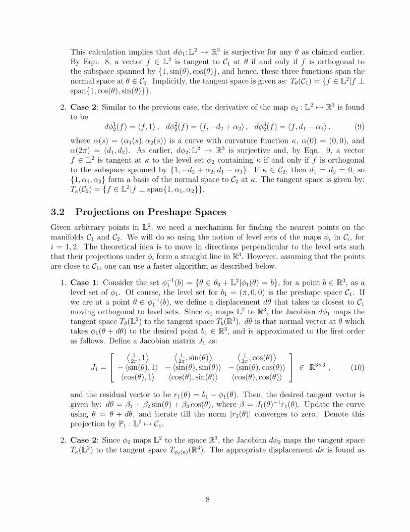
2. Case 2: Similar to the previous case, the derivative of the map φ2 : L2 7→ R

3 is foundto be

dφ12(f) = 〈f, 1〉 , dφ2

2(f) = 〈f,−d2 + α2〉 , dφ32(f) = 〈f, d1 − α1〉 . (9)

where α(s) = (α1(s), α2(s)) is a curve with curvature function κ, α(0) = (0, 0), andα(2π) = (d1, d2). As earlier, dφ2: L

2 → R3 is surjective and, by Eqn. 9, a vector

f ∈ L2 is tangent at κ to the level set φ2 containing κ if and only if f is orthogonal

to the subspace spanned by {1,−d2 + α2, d1 − α1}. If κ ∈ C2, then d1 = d2 = 0, so{1, α1, α2} form a basis of the normal space to C2 at κ. The tangent space is given by:Tκ(C2) = {f ∈ L

2|f ⊥ span{1, α1, α2}}.

3.2 Projections on Preshape Spaces

Given arbitrary points in L2, we need a mechanism for finding the nearest points on the

manifolds C1 and C2. We will do so using the notion of level sets of the maps φi in Ci, fori = 1, 2. The theoretical idea is to move in directions perpendicular to the level sets suchthat their projections under φi form a straight line in R

3. However, assuming that the pointsare close to C1, one can use a faster algorithm as described below.

1. Case 1: Consider the set φ−11 (b) = {θ ∈ θ0 + L

2|φ1(θ) = b}, for a point b ∈ R3, as a

level set of φ1. Of course, the level set for b1 = (π, 0, 0) is the preshape space C1. Ifwe are at a point θ ∈ φ−1

1 (b), we define a displacement dθ that takes us closest to C1

moving orthogonal to level sets. Since φ1 maps L2 to R

3, the Jacobian dφ1 maps thetangent space Tθ(L

2) to the tangent space Tb(R3). dθ is that normal vector at θ which

takes φ1(θ + dθ) to the desired point b1 ∈ R3, and is approximated to the first order

as follows. Define a Jacobian matrix J1 as:

J1 =

⟨12π

, 1⟩ ⟨

12π

, sin(θ)⟩ ⟨

12π

, cos(θ)⟩

−〈sin(θ), 1〉 − 〈sin(θ), sin(θ)〉 − 〈sin(θ), cos(θ)〉〈cos(θ), 1〉 〈cos(θ), sin(θ)〉 〈cos(θ), cos(θ)〉

∈ R

3×3 , (10)

and the residual vector to be r1(θ) = b1 − φ1(θ). Then, the desired tangent vector isgiven by: dθ = β1 + β2 sin(θ) + β3 cos(θ), where β = J1(θ)

−1r1(θ). Update the curveusing θ = θ + dθ, and iterate till the norm |r1(θ)| converges to zero. Denote thisprojection by P1 : L

2 7→ C1.

2. Case 2: Since φ2 maps L2 to the space R

3, the Jacobian dφ2 maps the tangent spaceTκ(L

2) to the tangent space Tφ2(κ)(R3). The appropriate displacement dκ is found as

8

follows. Define the Jacobian matrix

J2 =

2π 〈1, α1〉 〈1, α2〉

−2πd2 + 〈1, α2〉 − 〈d2, α1〉 + 〈α2, α1〉 − 〈d2, α2〉 + 〈α2, α2〉2πd1 + 〈1, α1〉 〈d1, α1〉 − 〈α1, α1〉 〈d1, α2〉 − 〈α1, α2〉

∈ R

3×3 .

(11)and the residual vector r2(κ) = b2 −φ2(κ), where b2 = (2π, 0, 0). Set dκ = β1 + β2α1 +β3α2, where β = J2(κ)−1r2(κ). Update using κ = κ+dκ and iterate till |r2(κ)| becomessmall enough. Denote this projection by P2 : L

2 7→ C2.

Shown in Figure 1 are some examples of projecting curves in the larger spaces to the preshapespaces.

−1 −0.5 0 0.5 1

0

0.2

0.4

0.6

0.8

1

1.2

1.4

1.6

−1 −0.5 0 0.5 1−0.6

−0.4

−0.2

0

0.2

0.4

0.6

0.8

1

1.2

1.4

−2 −1.5 −1 −0.5 0 0.5 1 1.5 2

−1

−0.5

0

0.5

1

1.5

2

−1.5 −1 −0.5 0 0.5 10

0.5

1

1.5

2

2.5

Figure 1: Examples of projecting curves onto preshape spaces. The first two panels are forC1 while the last two panels are for C2. Broken lines denote the original curves and solidlines draw the projected curves.

3.3 Geodesics On Preshape Spaces

Given two parameterized curves, they are represented by two points in a preshape space(C1 or C2). We wish to construct the “most efficient” deformation from one of these curvesto the other. A natural formulation of “most efficient” is simply to construct the shortestpath between the corresponding points in the preshape space with respect to the Riemannianmetric given by the L

2 inner product on the tangent space, i.e., a length-minimizing geodesic.We then define the “distance” between the parameterized curves to be the length of thisgeodesic. We remind the reader that a geodesic on a manifold embedded in a Euclideanspace is defined to be a constant speed curve on the manifold, whose acceleration vector isalways perpendicular to the manifold. It is known that given any two points on a completemanifold, there exists a shortest path between them, and that path is a geodesic. It is alsotrue that geodesics on a complete manifold can be extended infinitely far in both directions.(See for example [16].)

There are other approaches to interpolating between closed curves (see for example [23]).Our geodesic construction has several advantages: it is defined for all pairs of closed curves(not just relatively close ones), and it is guaranteed to give a path of closed curves. It isinteresting to ask whether, given two simple (i.e., with no self-crossings) closed curves, theinterpolating geodesic will always consist of simple closed curves. While we haven’t beenable to prove that it does, we haven’t found any counterexamples either.

One issue we need to mention about geodesics is that while geodesics are locally length-minimizing (i.e. for two points on the geodesic which are close together, the geodesic provides

9

the shortest path between them), our algorithm is not guaranteed to achieve the shortestgeodesic in a global sense. In other words, we have not proven that geodesics connectingany two shapes are unique. However, our experimental studies so far seem to support thathypothesis.

We now construct geodesic paths on the preshape spaces. We will approximate geodesicson C1 or C2 by taking small increments in the larger space (θ0+L

2 or L2), and then projecting

back to C1 or C2 using P1 or P2.

1. Case 1: Let θ ∈ C1, and f ∈ Tθ(C1) be a tangent vector. We want to generate a geodesicpath (generated by a one-parameter flow) starting from θ and with tangent vector fat θ; denote this flow by Ψ(θ, t, f) where t is the time parameter. We will evaluate thisflow for discrete times t = ∆, 2∆, 3∆, . . . , for a small ∆ > 0. Setting Ψ(θ, 0, f) = θ,take the first increment to reach θ+∆f in L

2 and apply the projection P1 to this point.Set Ψ(θ, ∆, f) = P1(θ + ∆f) to get the next point along the geodesic. Iterating thisprocess provides successive points along the geodesic Ψ in C1. One remaining issue isthat we need to transport the tangent vector f to the next point along the geodesic toperform iterations. This can be achieved by orthogonally projecting f to the tangentspace at the next point, thereby achieving a discrete version of the requirement thatthe acceleration vector of a geodesic should be perpendicular to the manifold. Afterprojecting f to the next tangent space, we renormalize it to keep the “speed” of thegeodesic constant. For example, let θ̃ be a point along the geodesic path; we wantto find f̃ that is tangent to C1 at θ̃ and is a parallel transport of f . This can beaccomplished using:

f̃ = ‖f‖ g

‖g‖ , where g = f −3∑

k=1

〈f, hk〉hk , (12)

and where hks form an orthonormal basis of the space span{1, cos(θ̃), sin(θ̃)}.An algorithm summarizing the steps for constructing a geodesic path on C1 is as follows:

Algorithm 1 Start with a point θ ∈ C1 and a direction f ∈ Tθ(C1). Set j = 0 andΨ(θ, j, f) = θ, and choose a small ∆ > 0.

(a) Compute the increment Ψ(θ, j∆, f)+∆f and set Ψ(θ, (j+1)∆, f) = P1(Ψ(θ, j∆, f)+∆f).

(b) Transport f to the new point by using Ψ(θ, (j + 1)∆, f) for θ̃ in Eqn. 12.

(c) Set j = j + 1. Go to step (a) with f = f̃ .

It can be shown that for ∆ → 0, Ψ converges to a geodesic path on C1.

2. Case 2: The construction of geodesics on C2 is similar to the previous case with thedirection functions replaced by the curvature functions. The only exception is that, inEqn. 12, the hks form an orthonormal basis of the space span{1, α1, α2}, where α is thecurve generated by the curvature function κ̃ at which the tangent is being transported.

10

3.4 Geodesics On Shape Spaces

Since the shape spaces S1 and S2 are the quotient spaces of the corresponding preshapespaces under actions of S

1 by isometries, the problem of finding geodesics in S1 and S2

reduces to the problem of finding geodesics in the corresponding preshape spaces which areorthogonal to the S

1 orbits. The fact that S1 acts by isometries also implies that if a geodesic

in a preshape space is orthogonal to one S1 orbit, then it is orthogonal to all S

1 orbits whichit meets and, hence, projects to a goedesic in the corresponding shape space.

1. Case 1: To find a geodesic in C1 which is orthogonal to the S1-orbits, we simply

restrict the allowable tangent directions to be orthogonal to the S1-orbits, i.e. use only

those f ∈ Tθ(C1) which are perpendicular to Tθ(S1(θ)). It can be shown that this one-

dimensional space is spanned by 1 − θ′, and hence, f should be orthogonal to 1 − θ′.(Here we restrict to those elements of C1 that have continuous first derivative.) Thealgorithm for constructing geodesics in S1 is identical to Algorithm 1 except that inEqn. 12 the vector g is now given by: g = f − ∑4

k=1 〈f, hk〉hk, where hks form an

orthonormal basis of the space span{1, cos(θ̃), sin(θ̃), 1 − θ̃′}.2. Case 2: The construction of geodesics on S2 is similar except that the basis of Tκ(S

1(κ))is given by κ′. Hence, Algorithm 1 applies except that in Eqn. 12 the hks form anorthonormal basis of the space span{1, α1, α2, κ

′}, where α = (α1, α2) is the curve gen-erated by the curvature function κ. Note the assumption that the curvature functionshave first derivatives.

4 Numerical Methods for Finding Geodesics

So far we have described a technique for approximating geodesic paths in the two shapespaces. However, the main task of finding a geodesic path between any two given shapesstill remains. This problem can be stated as follows:Problem Statement: Given two elements θ1, θ2 ∈ S1, or κ1, κ2 ∈ S2, how does oneconstruct a geodesic flow such that it starts from one and reaches the other, or a re-parametrization of the other, in unit time.

1. Case 1: Let Ψ be the desired one-parameter flow from θ1 to θ2. For any f ∈ Tθ1(S1),Algorithm 1 generates a geodesic path in S1. Therefore, the real issue is to find thatappropriate direction f ∈ Tθ1(S1) such that a geodesic in that direction passes throughthe S

1-orbit of θ2. In other words, the problem is to solve for an f ∈ Tθ1(C1) such thatΨ(θ1, 0, f) = θ1 and Ψ(θ1, 1, f) = s · θ2, for some s ∈ S

1. One can treat the searchfor this appropriate direction as an optimization problem over the Tθ1(S1). The costfunction for minimizing is given by the functional:

H[f ] = infs∈S1

‖Ψ(θ1, 1, f) − (s · θ2)‖2 , (13)

and we are looking for that f ∈ Tθ1(S1) for which: (i) H[f ] is zero and (ii) ‖f‖ isminimum among all such tangents. Since the space Tθ1(S1) is infinite dimensional, thisoptimization is not straightforward.

11

One idea is to use a finite-dimensional approximation of the elements of Tθ1(S1) to findthe optimal direction. Since f ∈ L

2, it has a Fourier decomposition and we can solvethe optimization problem over a finite number of Fourier coefficients. Approximateany f ∈ Tθ1(S1) according to f(s) ≈ ∑m

n=0(an cos(ns)+ bn sin(ns)), for a large positiveinteger m. The cost function modifies to: H̃ : R

2m+1 7→ R+,

H̃(a, b) = infs∈S1

‖Ψ(θ1, 1,m∑

n=0

an cos(ns) + bn sin(ns)) − (s · θ2)‖2 . (14)

The paper [19] describes an elegant technique to solve the inf part of the problem overthe reparametrization group using discrete Fourier transforms. We believe that thisapproach can be adopted here although we have not explored it further.

Shown in Figure 2 are three examples of geodesics between θ1 on the left and the targetshape θ2 on the right. Drawn in between are shapes denoting equally spaced pointsalong the geodesic paths. We emphasize that because of our restriction that θ hasaverage value π on [0, 2π], and because our algorithm produces geodesics which areperpendicular to the S

1-orbits, the initial alignment of the two curves is completelyautomatic. For example in the top panel, the bird and bottle shapes are rotationallyaligned to produce a geodesic which cannot be made any shorter by a small rotationalre-alignment. Also, the search for the optimal tangent is fast; it takes less than threeseconds on a Pentium III processor in a matlab environment when T = 100 and m = 50.

2. Case 2: Shown in Figure 3 are similar examples of the geodesic paths in S2.

5 Applications of Shape Analysis

There are many interesting applications of the shape representations and metrics that we haveproposed. An important advantage of our approach is that it provides geodesic paths betweenthe shapes on the shape spaces. These paths can be used to interpolate between shapes,extrapolate a shape change, and compute a mean shape under a probability distributionon shapes. Furthermore, it can lead to tools for sophisticated statistical inferences suchas confidence interval estimation, hypothesis testing, and Monte Carlo techniques on suchshape spaces.

To illustrate these ideas, we will describe three applications: (i) interpolations and ex-trapolations in shape spaces , (ii) clustering of planar objects according to their shapes, and(ii) computation of sample statistics, such as mean and variance, for some given shapes. Wealso suggest some simple probability distributions on the shape manifold for use in futurestatistical extraction of shapes from images.

To demonstrate our ideas, we have utilized a database of fish shapes generated by theresearchers at Univ of Surrey, UK [21]. This database consists of the boundary points ofapproximately 1100 marine creatures, each hand-extracted from their pictures. Before wedescribe these applications, we discuss some implementation issues:

12

0 2 4 6 8 10 12

0

1

2

0 2 4 6 8 10 12

0

1

2

0 2 4 6 8 10 12

0

1

2

Figure 2: Examples of evolving one shape into another via a geodesic path. Leftmost shapeis θ1, rightmost curves are θ2, and nine intermediate shapes are equispaced points along thegeodesic.

1. Data Pre-Processing: We have represented shapes via their direction functions θ ∈S1 or the curvature functions κ ∈ S2. However, the available coordinate data mayneither be uniformly sampled nor have the required curve length. Therefore, we needto preprocess the raw data to obtain an appropriate representation of each shape.

Let pi ∈ R2, i = 1, 2, . . . , k be an ordered collection of points on an objects’ boundary.

Define the chord lengths δi = ‖pi+1 − pi‖, i = 1, 2, . . . , k − 1 and set tj =∑j

i=1 δi for

j = 1, . . . , k−1. For φi = tan−1(pi+1(2)−pi(2)pi+1(1)−pi(1)

), we get a collection {ti, φi} of k−1 nodes,

and we fit a locally-smooth function, such as a spline, through these nodes. We can nowresample this function uniformly for the desired number of points, call that number T .Fixing the spacing between these points to be δ = 2π

T, and forcing its mean value to

be π, we can obtain a representation θ ∈ S1. Taking its derivative provides a κ ∈ S2.Coordinate function for this shape can be obtained using αi+1 = αi + exp(−jθi)δ.Figure 4 shows some examples of the pre-processing: for each pair the left panels showthe original data and the right panels show the shapes after smoothing and re-sampling.These examples involve a significant reduction in data points: top left is a reductionfrom 1037 points to 100 points, bottom right is from 611 to 100 points.

2. Inner Products: The inner product between two tangent functions is approximatedusing the finite sum: 〈f1, f2〉 =

∫ 2π

0f1(s)f2(s)ds ≈ ∑T

i=1 f1(iδ)f2(iδ)δ, where δ = 2π/T .

13

0 5 10 15

0

1

2

0 5 10 15

0

1

2

Figure 3: Evolution of shapes along geodesic paths in S2

.

50 100 150 200 250 300

0

50

100

150

200

0 0.2 0.4 0.6 0.8 1 1.2 1.4 1.6

−0.6

−0.4

−0.2

0

0.2

0.4

0.6

20 40 60 80 100 120

20

30

40

50

60

70

80

90

100

0 0.2 0.4 0.6 0.8 1

−0.6

−0.5

−0.4

−0.3

−0.2

−0.1

0

0.1

0.2

0.3

−100 −50 0 50 100 150 200 250 300

50

100

150

200

250

300

350

−0.5 0 0.5 1 1.5−1

−0.8

−0.6

−0.4

−0.2

0

0.2

0.4

0.6

0.8

s 0 50 100 15020

40

60

80

100

120

140

160

180

200

−0.5 0 0.5 1 1.5

−0.8

−0.6

−0.4

−0.2

0

0.2

0.4

0.6

0.8

Figure 4: Object boundaries before and after preprocessing.

5.1 Interpolation and Extrapolation on Shape Spaces

Interpolation between shapes is useful in several applications. As an example, given twoparallel slices of a 3D scan of an anatomical shape, we may want to find a surface that bestinterpolates between the given shapes. Also, in the case of time varying shapes, one may beinterested in estimating intermediate shapes given shapes at two different times. Similarly,given an observed sequence of time-varying shapes, one may be interested in predicting afuture shape following similar shape changes, and tools for shape extrapolation are needed.We demonstrate the use of geodesic flows in shape interpolation and extrapolation. Shownin Figure 5 is a geodesic path in S1 between the two fishes drawn in bold lines. Shapes inbetween the two can be used to interpolate between them, and the shapes on the right canbe used to predict future shapes along that path.

14

0 5 10 15 20

0

1

2

3

Figure 5: Interpolation and extrapolation on the shape space given the two shapes drawn inbold lines.

5.2 Clustering and Recognition of Shapes

In many applications, the goal is to classify and cluster objects according to their shapes.Examples include object classification, shape-based database searches, and object detectionin images.

We first compute geodesic paths between two shapes, and then compute the lengths ofthe optimal tangent vectors to find the geodesic lengths. We have computed this geodesiclength pairwise for a subset of the database containing 16 fishes shown in Figure 6. In

0 0.5 1 1.5 2

−1

−0.8

−0.6

−0.4

−0.2

0

0.2

0.4

0.6

0.8

−0.5 0 0.5 1 1.5

−0.8

−0.6

−0.4

−0.2

0

0.2

0.4

0.6

0.8

−1 −0.5 0 0.5 1 1.5

0

0.5

1

1.5

−1 −0.5 0 0.5 1 1.5

−1.5

−1

−0.5

0

0.5

−0.5 0 0.5 1 1.5

−0.8

−0.6

−0.4

−0.2

0

0.2

0.4

0.6

0.8

−1 −0.5 0 0.5 1 1.5

0

0.5

1

1.5

2

0 0.5 1 1.5

−0.8

−0.6

−0.4

−0.2

0

0.2

0.4

−0.5 0 0.5 1 1.5 2−1

−0.8

−0.6

−0.4

−0.2

0

0.2

0.4

0.6

0.8

1

−0.5 0 0.5 1 1.5 2

−1

−0.5

0

0.5

1

−1 −0.5 0 0.5 1 1.5

−1

−0.5

0

0.5

1

−0.5 0 0.5 1 1.5

−0.8

−0.6

−0.4

−0.2

0

0.2

0.4

0.6

0.8

0 0.2 0.4 0.6 0.8 1 1.2 1.4 1.6

−0.6

−0.4

−0.2

0

0.2

0.4

0.6

0 0.5 1 1.5 2 2.5

−1

−0.8

−0.6

−0.4

−0.2

0

0.2

0.4

0.6

0.8

0 0.2 0.4 0.6 0.8 1 1.2 1.4 1.6

−0.6

−0.4

−0.2

0

0.2

0.4

0.6

−1 −0.5 0 0.5 1 1.5

−1

−0.8

−0.6

−0.4

−0.2

0

0.2

0.4

0.6

0.8

1

−0.5 0 0.5 1 1.5 2

−1

−0.5

0

0.5

1

Figure 6: Sixteen sample fish contours taken from Surrey fish database The shapes arenumbered from top left to bottom right with successive numbers along rows

this implementation, we have used 50 Fourier components to represent the tangent vectors.To illustrate the task of clustering objects using this metric, we have applied a clusteringalgorithm described in [9] to the 16 shapes shown in Fig 6. Seeking seven clusters, the resultis shown in the Figure 7. Each row in the figure represents a cluster with the last panelsshowing the cluster means (to be defined later in Section 5.3.1). The choice of number ofclusters can be based on a complexity penalty [9] or on a mixture model [6].

15

−0.5 0 0.5 1 1.5

−0.8

−0.6

−0.4

−0.2

0

0.2

0.4

0.6

0.8

−0.5 0 0.5 1 1.5

−0.8

−0.6

−0.4

−0.2

0

0.2

0.4

0.6

0.8

−0.5 0 0.5 1 1.5

−0.8

−0.6

−0.4

−0.2

0

0.2

0.4

0.6

0.8

−0.5 0 0.5 1 1.5 2−1

−0.8

−0.6

−0.4

−0.2

0

0.2

0.4

0.6

0.8

1

0 0.5 1 1.5 2

−1

−0.8

−0.6

−0.4

−0.2

0

0.2

0.4

0.6

0.8

0 0.5 1 1.5 2 2.5

−1

−0.8

−0.6

−0.4

−0.2

0

0.2

0.4

0.6

0.8

1

−0.5 0 0.5 1 1.5

−0.8

−0.6

−0.4

−0.2

0

0.2

0.4

0.6

0.8

−0.5 0 0.5 1 1.5

−0.8

−0.6

−0.4

−0.2

0

0.2

0.4

0.6

0.8

1

0 0.5 1 1.5 2 2.5

−1

−0.8

−0.6

−0.4

−0.2

0

0.2

0.4

0.6

0.8

0 0.5 1 1.5 2 2.5−1.2

−1

−0.8

−0.6

−0.4

−0.2

0

0.2

0.4

0.6

0.8

−1 −0.5 0 0.5 1 1.5

−1

−0.8

−0.6

−0.4

−0.2

0

0.2

0.4

0.6

0.8

1

−1 −0.5 0 0.5 1 1.5

−1.5

−1

−0.5

0

0.5

−1 −0.5 0 0.5 1 1.5

−1

−0.5

0

0.5

1

−1 −0.5 0 0.5 1 1.5

−1

−0.5

0

0.5

1

0 0.2 0.4 0.6 0.8 1 1.2 1.4 1.6

−0.6

−0.4

−0.2

0

0.2

0.4

0.6

0 0.2 0.4 0.6 0.8 1 1.2 1.4 1.6

−0.6

−0.4

−0.2

0

0.2

0.4

0.6

0 0.5 1 1.5

−0.8

−0.6

−0.4

−0.2

0

0.2

0.4

0 0.2 0.4 0.6 0.8 1 1.2 1.4 1.6 1.8

−0.4

−0.2

0

0.2

0.4

0.6

0.8

−0.5 0 0.5 1 1.5 2

−1

−0.5

0

0.5

1

−1 −0.5 0 0.5 1 1.5

0

0.5

1

1.5

−1 −0.5 0 0.5 1 1.5

0

0.5

1

1.5

2

−0.5 0 0.5 1 1.5 2

−1

−0.5

0

0.5

1

−1 −0.5 0 0.5 1 1.5 2

−1

−0.5

0

0.5

1

Figure 7: Fish shapes distributed among 7 row-wise clusters with the cluster means shownin the final column.

5.3 Statistical Analysis of Shapes

Similar to the ideas in [5], our future interest lies in Bayesian inferences on shapes given noisy(perhaps image-based) data. Towards that goal we are interested in imposing probabilitydistributions on the shape spaces S1 and S2, with techniques for computing mean shapes andvariances around mean shapes. The Riemannian structures on these shape spaces enable usto perform such a statistical analysis. In the interest of brevity, we describe the proceduresonly for S1; S2 can be handled similarly.

5.3.1 Computation of Mean Shapes

There are at least two ways of defining a “mean” value for a random variable that takesvalues on S1. The first definition, called extrinsic mean, involves embedding the manifold ina vector space, computing the Euclidean mean in that space, and then projecting it downto the manifold [1, 27]. The other definition, called the intrinsic mean or the Karcher mean([1, 31, 10, 13]) does not require a Euclidean embedding. Let d(θi, θj) denote the length of theshortest geodesic from θi to θj in S1. To calculate the Karcher mean of shapes {θ1, . . . , θn}

16

in S1, define the variance function V : S1 → R by V (θ) =∑n

i=1 d(θ, θi)2. Then, define the

Karcher mean of the given shapes to be any point µ ∈ S1 for which V (µ) is a local minimum.In the case of Euclidean spaces this definition agrees with the usual definition µ = 1

n

∑ni=1 pi.

Since S1 is complete, the intrinsic mean as defined above always exists. However, there maybe certain sets of points for which µ is not unique.We now review the algorithm given in [31] for finding a Karcher mean for a given set ofpoints. If the points {θ1, . . . , θn} are clustered fairly close together (relative to the curvatureof S1), it has been proven that the Karcher mean exists, is unique, and can be found by thefollowing gradient search algorithm. (See the papers mentioned above for details.)

Algorithm 2 Set k = 0. Choose some time increment ε ≤ 1n. Choose a point µ0 ∈ S1 as

an initial guess of the mean. (For example, one could just take µ0 = θ1.)

1. For each i = 1, . . . , n choose the tangent vector fi ∈ Tµk(S1) which is tangent to the

shortest geodesic from µk to θi, and whose norm is equal to the length of this shortestgeodesic. The vector g =

∑ni=1 fi is equal to (−2) times the gradient at µk of the

function V : S1 → R which we defined above.

2. Flow for time ε along the geodesic which starts at µk and has velocity vector g. Callthe point where you end up µk+1, i.e. µk+1 = Ψ(ε, µk, g).

3. Set k = k + 1, and go to Step 1.

A similar algorithm and convergence results for a landmark-based representation of shapesare described in [18]. Instead of a finite set of shapes, we may be given a probabilitydistribution on S1, and wish to calculate its intrinsic mean. In this case the sum of tangentvectors in Step 1 must be replaced by an integral over the tangent space. Shown in Figure8 are three examples of computing the Karcher mean shapes: the left four panels show thesample shapes and the rightmost panels display the corresponding mean shapes. Additionalexamples are shown in Figure 7.

5.3.2 Variances on Shape Spaces

Having defined a mean shape, the definition of covariance follows. Rather than defininga covariance operator over the manifold S1, we restrict ourselves only to a scalar quantitymeasuring the amount of variability associated with a probability density on S1. For theprobability density P , let µ be the intrinsic mean shape as defined above. Then, for any [θ] ∈S1, define fθ ∈ Tµ(C1) to be the tangent direction at µ that leads to a geodesic connecting µand to the S

1-orbit of θ, which is orthogonal to these S1-orbit of µ. If θ1, θ2, . . . , θn are samples

from a probability distribution, then the sample variance is estimated as: ρ̂ = 1n

∑ni=1 ‖fθi‖2.

For example, ρ̂ = 2.808 for the four fishes shown in the (first four) middle panels of Figure8.

5.3.3 Probability Distributions on Shape Spaces

An important issue for statistical analysis of shapes is the definition of a probability measureon the preshape space C1 or the shape space S1. Given a reference measure, or a base measure

17

−0.5 0 0.5 1 1.5−0.4

−0.2

0

0.2

0.4

0.6

0.8

1

1.2

1.4

1.6

−1 −0.5 0 0.5 1 1.5

0

0.5

1

1.5

2

−1 −0.5 0 0.5 10

0.2

0.4

0.6

0.8

1

1.2

1.4

1.6

1.8

2

−1 −0.5 0 0.5 1 1.50

0.2

0.4

0.6

0.8

1

1.2

1.4

1.6

1.8

2

−1.5 −1 −0.5 0 0.5 1 1.50

0.5

1

1.5

2

2.5

−1 −0.5 0 0.5 1

−0.4

−0.2

0

0.2

0.4

0.6

0.8

−1 −0.5 0 0.5 1

−0.6

−0.4

−0.2

0

0.2

0.4

0.6

0.8

1

−1 −0.5 0 0.5 1

−0.4

−0.2

0

0.2

0.4

0.6

0.8

1

1.2

−1 −0.8 −0.6 −0.4 −0.2 0 0.2 0.4 0.6 0.8 1−0.5

0

0.5

1

−1 −0.5 0 0.5 1

−0.6

−0.4

−0.2

0

0.2

0.4

0.6

0.8

1

1.2

−1 −0.8 −0.6 −0.4 −0.2 0 0.2 0.4 0.6 0.8 10

0.2

0.4

0.6

0.8

1

1.2

1.4

1.6

1.8

−1 −0.5 0 0.5 10

0.5

1

1.5

2

−1 −0.5 0 0.5 10

0.2

0.4

0.6

0.8

1

1.2

1.4

1.6

1.8

−1 −0.5 0 0.5 10

0.2

0.4

0.6

0.8

1

1.2

1.4

1.6

1.8

2

−1 −0.5 0 0.5 10

0.2

0.4

0.6

0.8

1

1.2

1.4

1.6

1.8

2

Figure 8: Karcher means (right panels) of the four shapes given in left panels for each row.

on these spaces, only the probability density P remains to be specified. There are severalways of defining probability densities on these spaces. One way is to select a mean shapeµ ∈ S1 and impose a probability density on the tangent (vector) space Tµ(S1). This measurecan be inherited by S1 via the geodesic flow, f ∈ Tµ(S1) 7→ Ψ(1, µ, f) ∈ S1.

Let Ψ−1µ (θ) denote a point in Tµ(S1) such that Ψ(1, µ, Ψ−1(θ)) = θ. Now, if h(f) is a

probability density function on the vector space Tµ(S1), then the density inherited on S1

can be defined as: Pµ(θ) ∝ h(Ψ−1µ (θ)). It is difficult to compute the normalization constant

of P . Therefore, it is natural to use Monte Carlo techniques to generate inferences from fsince they do not require the normalization constant. Shown in Figure 9 is an example ofsampling from such a probability.

−1 −0.8 −0.6 −0.4 −0.2 0 0.2 0.4 0.6 0.8 1−0.6

−0.4

−0.2

0

0.2

0.4

0.6

0.8

1

−1 −0.8 −0.6 −0.4 −0.2 0 0.2 0.4 0.6 0.8

−0.2

0

0.2

0.4

0.6

0.8

1

1.2

−1 −0.8 −0.6 −0.4 −0.2 0 0.2 0.4 0.6 0.8

−0.2

0

0.2

0.4

0.6

0.8

1

1.2

−1 −0.8 −0.6 −0.4 −0.2 0 0.2 0.4 0.6 0.8

−0.4

−0.2

0

0.2

0.4

0.6

0.8

1

Figure 9: Right panels show three random shapes generated from a probability model withthe mean shape shown in the leftmost panel.

Hypothesis Testing: A common problem in shape classification to test whether the ob-served shape belongs to one class or the other. If one can specify the two classes according tothe probability models Pµ1(θ) and Pµ1(θ), then select the hypothesis according to the ratio:Pµ1 (θ)

Pµ2 (θ). One needs to study the effectiveness of this test on extensive databases.

18

6 Summary & Discussion

In this paper we have described two geometric representations of planar shapes using: (i)direction functions and (ii) curvature functions. The resulting shape spaces are studied asspaces with finite co-dimensions inside L

2 and its translation. Utilizing the underlying geom-etry of these shape spaces, we solve a shooting problem for connecting two arbitrary shapesvia geodesic paths and set the geodesic lengths as a metric between shapes. This approachhas many applications, three of them studied here are: (i) interpolating and extrapolating inshape spaces, (ii) clustering of objects according to their shapes, and (iii) computing meansand variances of shapes. Using fish shapes from Surrey fish database, we have demonstratedthese three applications.

There are three different “discretizations” used in this approach: (i) approximation ofcontinuous geodesics by discretized paths, with a step size of ∆ (Section 3.3), (ii) approxi-mation of tangent functions f(s) ∈ Tθ1(S) by their Fourier representation (Section 4), and(iii) approximation of the direction functions θ(s) by uniformly spaced samples (Section 5,pre-processing). The strategy for choosing the discretization parameters is straightforward:choose them as finely as you can keeping in mind the resulting computational complexity.Beyond a certain stage the improvement in performance will be overtaken by the increase incomputational cost.

Our choice of metric on shape spaces relates to measuring the “bending” energy in chang-ing one shape to another. Similar to the ideas presented in [23], we would like an extensionthat measures a combination of bending and stretching energies, and bases inferences on thisframework.

Acknowledgments

The authors would like to thank Mr. Shantanu Joshi for his help in generating the clusteringresults. This research has been supported in part by the grants NSF DMS-0101429, ARODAAD19-99-1-0267, and NMA 201-01-2010.

References

[1] R. Bhattacharya and V. Patrangenaru. Nonparametric estimation of location and dis-persion on riemannian manifolds. Journal for Statistical Planning and Inference, 108:23–36, 2002.

[2] F. L. Bookstein. Size and shape spaces for landmark data in two dimensions. StatisticalScience, 1:181–242, 1986.

[3] M. P. Do Carmo. Differential Geometry of Curves and Surfaces. Prentice Hall, Inc.,1976.

[4] I. Cohen and I. Herlin. Tracking meteorological structures through curve matching usinggeodesic paths. In Proceedings of ICCV, pages 396–401, 1998.

19

[5] I. L. Dryden and K. V. Mardia. Statistical Shape Analysis. John Wiley & Son, 1998.

[6] M. A. T. Figueiredo and A. K. Jain. Unsupervised learning of finite mixture models.IEEE Transactions on Pattern Analysis and Machine Intelligence, 24(3), 2002.

[7] U. Grenander. General Pattern Theory. Oxford University Press, 1993.

[8] U. Grenander and M. I. Miller. Computational anatomy: An emerging discipline. Quar-terly of Applied Mathematics, LVI(4):617–694, 1998.

[9] S. Joshi and A. Srivastava. An algorithm for clustering objects according to their shapes.Monograph of Department of Statistics, Florida State University, 2003.

[10] H. Karcher. Riemann center of mass and mollifier smoothing. Communications on Pureand Applied Mathematics, 30:509–541, 1977.

[11] M. Kass, A. Witkin, and D. Terzopoulos. Snakes: Active contour models. InternationalJournal of Computer Vision, 1:321–331, 1988.

[12] David G. Kendall. Shape manifolds, procrustean metrics and complex projective spaces.Bulletin of London Mathematical Society, 16:81–121, 1984.

[13] W. S. Kendall. Probability, convexity, and harmonic maps with small image I: Unique-ness and fine existence. Proceedings of the London Mathematical Society, 61:371–406,1990.

[14] J. T. Kent. New directions in shape analysis. In K. V. Mardia, editor, The Art ofStatistical Science, pages 115–127. John Wiley and Sons Ltd, 1992.

[15] N. Khaneja, M.I. Miller, and U. Grenander. Dynamic programming generation of curveson brain surfaces. IEEE Transactions on Pattern Analysis and Machine Intelligence,20(11):1260–1264, Nov 1998.

[16] S. Lang. Fundamentals of Differential Geometry. Springer, 1999.

[17] L. J. Latecki, R. Lakamper, and U. Eckhardt. Shape descriptors for non-rigid shapeswith a single closed contours. In IEEE Conf. on Computer Vision and Pattern Recog-nition, pages 424–429, 2000.

[18] H. Le. Locating frechet means with application to shape spaces. Advances in AppliedProbability, 33(2):324–338, 2001.

[19] J. S. Marques and A. J. Abrantes. Shape alignment - optimal initial point and poseestimation. Pattern Recognition Letters, 18:49–53, 1997.

[20] M. I. Miller and L. Younes. Group actions, homeomorphisms, and matching: A generalframework. International Journal of Computer Vision, 41(1/2):61–84, 2002.

[21] F. Mokhtarian, S. Abbasi, and J. Kittler. Efficient and robust shape retrieval by shapecontent through curvature scale space. In Proceedings of First International Conferenceon Image Database and MultiSearch, pages 35–42, 1996.

20

[22] R. S. Palais. Morse theory on hilbert manifolds. Topology, 2:299–340, 1963.

[23] T. B. Sebastian, P. N. Klein, and B. B. Kimia. On aligning curves. IEEE Transactionson Pattern Analysis and Machine Intelligence, 25(1):116–125, 2003.

[24] T. W. Sederberg. A physically based approach to 2-d shape blending. Computer Graph-ics (Proceedings of Siggraph), 26(2):25–34, 1992.

[25] J. Sethian. Level Set Methods: Evolving Interfaces in Geometry, Fluid Mechanics,Computer Vision, and Material Science. Cambridge University Press, 1996.

[26] Christopher G. Small. The Statistical Theory of Shape. Springer, 1996.

[27] A. Srivastava and E. Klassen. Monte carlo extrinsic estimators for manifold-valuedparameters. IEEE Trans. on Signal Processing, 50(2):299–308, February 2001.

[28] H. D. Tagare, D. O’Shea, and D. Groisser. Non-rigid shape comparison of plane curvesin images. Journal of Mathematical Imaging and Vision, 16:57–68, 2002.

[29] D. W. Thompson. On Growth and Form: The Complete Revised Edition. Dover, 1992.

[30] A. Trouve. Diffemorphisms groups and pattern matching in image analysis. Interna-tional Journal of Computer Vision, 28(3):213–221, 1998.

[31] R. P. Woods. Characterizing volume and surface deformations in an atlas framework.Technical Report, Department of Neurology and Physiology, UCLA, 2002.

[32] L. Younes. Computable elastic distance between shapes. SIAM Journal of AppliedMathematics, 58:565–586, 1998.

[33] L. Younes. Optimal matching between shapes via elastic deformations. Journal of Imageand Vision Computing, 17(5/6):381–389, 1999.

21