Analysis of Plankton Populations

Sean Li

September 21, 2005

Abstract

I use numerical and analytical techniques to study the dynamicsof various models of plankton food webs with and without resourcefluctuations. Plankton are ideal organisms because they are verysmall, fast-reproducing organisms so they can easily be used in lab-oratory experiments to verify any results. We can study simple foodwebs to develop a better understanding of more complex food webs.The three archetypical food webs are a single grazer with a resource(growth), multiple grazers with a common resource (competition), andone grazer and one predator with a base resource (predator-prey).

1 Background

Plankton are microbial organisms that live in aquatic environments. Thereare two types of plankton: phytoplankton and zooplankton. Phytoplanktonare autotrophic organisms that use photosynthesis to generate their own foodfrom sunlight, water, and various nutrients. Zooplankton are heterotrophicorganisms that use phytoplankton as food sources themselves [2]. To under-stand the dynamics of the phytoplankton-zooplankton systems, one coulduse the analogy of self-sustaining plants and the animals that graze on them.

In 1961, Hutchinson presented the paradox of the plankton: ”The prob-lem that is presented by the phytoplankton is essentially how it is possiblefor a number of species to coexist in a relatively isotropic or unstructuredenvironment all competing for the same sorts of materials [1]”. Hutchinsonhypothesized that different species of plankton can coexist if they exploiteddifferences in other factors, such as efficiency of resource consumption underdifferent levels of resources.

1

One can model phytoplankton as one of two archetypes: gleaners andopportunists. Gleaner plankton thrive on low food levels (such as dim light)whereas opportunist plankton thrive on high food levels (such as bright light).As a result, opportunists tend to grow faster than gleaners because resourcesare usually abundant in the beginning of growth periods when phytoplanktonlevels are low. After both species reach their growth potential, resources be-come limited, and the gleaner becomes the dominant species. Figure 1 illus-trates this trait. While it is more realistic to look at the gleaner-opportunisttrait as a continuum rather than rigid archetypes, the simplistic binary char-acterization that we employ can prove insightful. Nevertheless, Planktonare only opportunist or gleaners relative to other species of plankton [3]. Itis also possible for one species of plankton to outperform another in all re-source regimes if it has a higher maximum intake (the maximum amountof resource a species can consume) and lower half-saturation (the point atwhich the resource intake is at its half capacity).

In addition to helping control the amount of carbon dioxide in the envi-ronment, phytoplankton also form the base of many food chains in aquaticecosystems [2]. Because phytoplankton are so integral to the overall healthof its environment, it is important to study the changes in their populationcaused by different ecological conditions such as fluctuating resources andthe introduction of other plankton species. In addition, plankton are idealorganisms to study because they are easy to conduct experiments with dueto their high growth rate, short life span, and small size [2].

The rest of this paper is organized as follows. We first look at the competi-tion model and find its equilibrium populations. Then we introduce resourcefluctuations and observe what happens when the period of the resource isadjusted (Section 3). We move on to the unforced chain model consistingof one phytoplankton population and one zooplankton population. We be-gin by finding a way to calculate the bifurcation points, special parametervalues that cause a qualitative change in the system’s dynamical behaviorif changed [4]. Then we find a way to approximate the time series of thesystem for parameter regimes close to the bifurcation point (Section 4). Weconclude by discussing our work (Section 5).

2

2 The Model

Working on the assumption that the plankton populations are well-mixed intheir environment with no population drifts, one can remove the system’sspatial dependence (a term representing diffusion of plankton from high den-sity areas to low density area), leaving only the temporal dependence. Thisallows us to model the time-dependent system using ordinary differentialequations (ODE) rather than partial differential equations.

One can use the following system of ODEs to model a system of phyto-plankton and zooplankton

Pi = cpigi(R)Pi − mpi

Pi − hj(Pi)Zj,

Zj = czjhj(P )Zj − mzj

Zj (1)

Here, Pi, Zj, and R denote phytoplankton population i, zooplankton pop-ulation j, and the resource (sunlight, water, etc.) respectively. As Pi and Zj

are not necessarily integers, letting them represent discrete plankton organ-isms does not make sense. Rather, we view them as populations densities,which allow non-integer values. The nutrient yield from consumption anddeath rates of species i are ci and mi, respectively. The plankton’s consump-tion functions, which indicate how much resource is processed for nutrition,are represented by gi(x) and hj(x) and modelled by the Monod function [2]

fn(x) =vnx

x + kn

, (2)

where kn and vn denote the half saturation rate and the maximum intakeof resource by species n, respectively. This functional response, which hasa limit to the maximum intake, is called a type II response. The type Ifunctional response, which does not consider a maximum limit on resourceintake can be modelled by the simplified Monod function: f(x) = vx/k [2].The type II functional response is the more realistic model, but the differ-ence in consumption between the two models is small in systems consistingof plankton with high maximum intake or low amounts of resources. Inthese situations, a type I response may be implemented to make the analysistractable.

The gleaner and opportunist archetypes only make sense in systems thathave type II functional responses. In a system of two competing type Iplankton, one species always outperforms the other because of the linearnature of the responses.

3

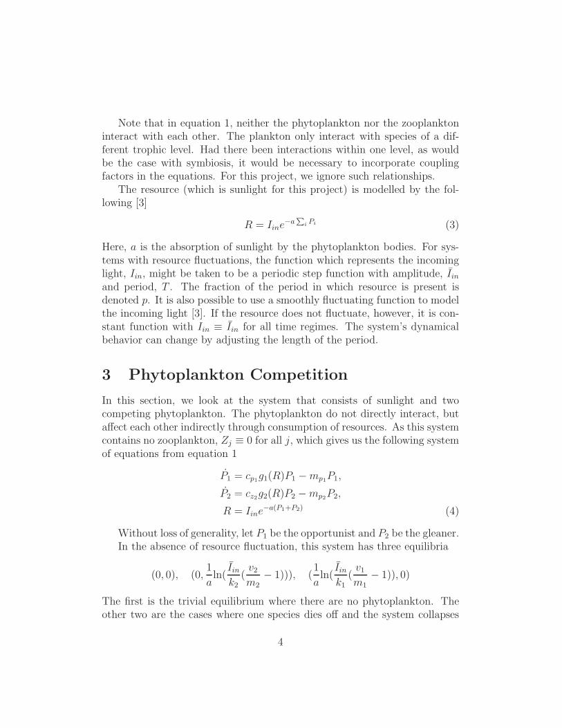
Note that in equation 1, neither the phytoplankton nor the zooplanktoninteract with each other. The plankton only interact with species of a dif-ferent trophic level. Had there been interactions within one level, as wouldbe the case with symbiosis, it would be necessary to incorporate couplingfactors in the equations. For this project, we ignore such relationships.

The resource (which is sunlight for this project) is modelled by the fol-lowing [3]

R = Iine−a

P

i Pi (3)

Here, a is the absorption of sunlight by the phytoplankton bodies. For sys-tems with resource fluctuations, the function which represents the incominglight, Iin, might be taken to be a periodic step function with amplitude, Iin

and period, T . The fraction of the period in which resource is present isdenoted p. It is also possible to use a smoothly fluctuating function to modelthe incoming light [3]. If the resource does not fluctuate, however, it is con-stant function with Iin ≡ Iin for all time regimes. The system’s dynamicalbehavior can change by adjusting the length of the period.

3 Phytoplankton Competition

In this section, we look at the system that consists of sunlight and twocompeting phytoplankton. The phytoplankton do not directly interact, butaffect each other indirectly through consumption of resources. As this systemcontains no zooplankton, Zj ≡ 0 for all j, which gives us the following systemof equations from equation 1

P1 = cp1g1(R)P1 − mp1

P1,

P2 = cz2g2(R)P2 − mp2

P2,

R = Iine−a(P1+P2) (4)

Without loss of generality, let P1 be the opportunist and P2 be the gleaner.In the absence of resource fluctuation, this system has three equilibria

(0, 0), (0,1

aln(

Iin

k2

(v2

m2

− 1))), (1

aln(

Iin

k1

(v1

m1

− 1)), 0)

The first is the trivial equilibrium where there are no phytoplankton. Theother two are the cases where one species dies off and the system collapses

4

into the growth model. As there are no non-trivial solutions for the equationsabove when the derivatives are set to 0, there can be no coexistence in asystem without resource fluctuation. Which equilibrium point the systemmoves towards depends on both the initial conditions and the parametervalues.

Upon introduction of resource fluctuation, the system exhibits more in-teresting dynamics. As shown figure 1, two types of behavior can occur. For

0 10 20 30 400

20

40

60

80

100

120

Time (T=1 days)

Pla

nkto

n P

opul

atio

n

OpportunistGleaner

0 1 2 3 4 5 60

20

40

60

80

100

120

140

Time (T=40 days)

Pla

nkto

n P

opul

atio

nOpportunistGleaner

0 1 2 3 4 5 60

20

40

60

80

100

120

140

Time (T=500 days)

Pla

nkto

n P

opul

atio

n

OpportunistGleaner

(a) (b) (c)

Figure 1: Plankton times series under resource fluctuation. One unit of timerepresents one period. In (a), the period is 1 day. In (b), the period is 40days. In (c), the period is 500 days. Note in (a), the opportunist dies offwhereas in (b) both species coexist.

resource fluctuations of very small periods (figure 1a), the overall behaviorof the system does not change. The system moves towards equilibrium, andone of the phytoplankton species dies off. For resource fluctuations of suffi-ciently large periods (figures 1bc), however, coexistence of both phytoplank-ton species becomes possible. In addition, the system exhibits a stable limitcycle, a periodic curve which contains a damping term that causes all nearbytime series to converge to the curve. In the long period case, we can treat theplankton populations as periodic multi-step functions. This method allowsus to analytically determine many qualities about the system [3]. Whetheror not coexistence is possible depends on parameter values. We focus onlyon situations in which there is coexistence. Observe that, in the intervals inwhich there is light, the growth patterns of the plankton behave as expected.The opportunist is the first species to dominate as there is a large amountof resource at the beginning of the period. Then after some time, the phyto-plankton population becomes sufficiently high and resources become scarcecausing dominance to shift to the gleaner.

5

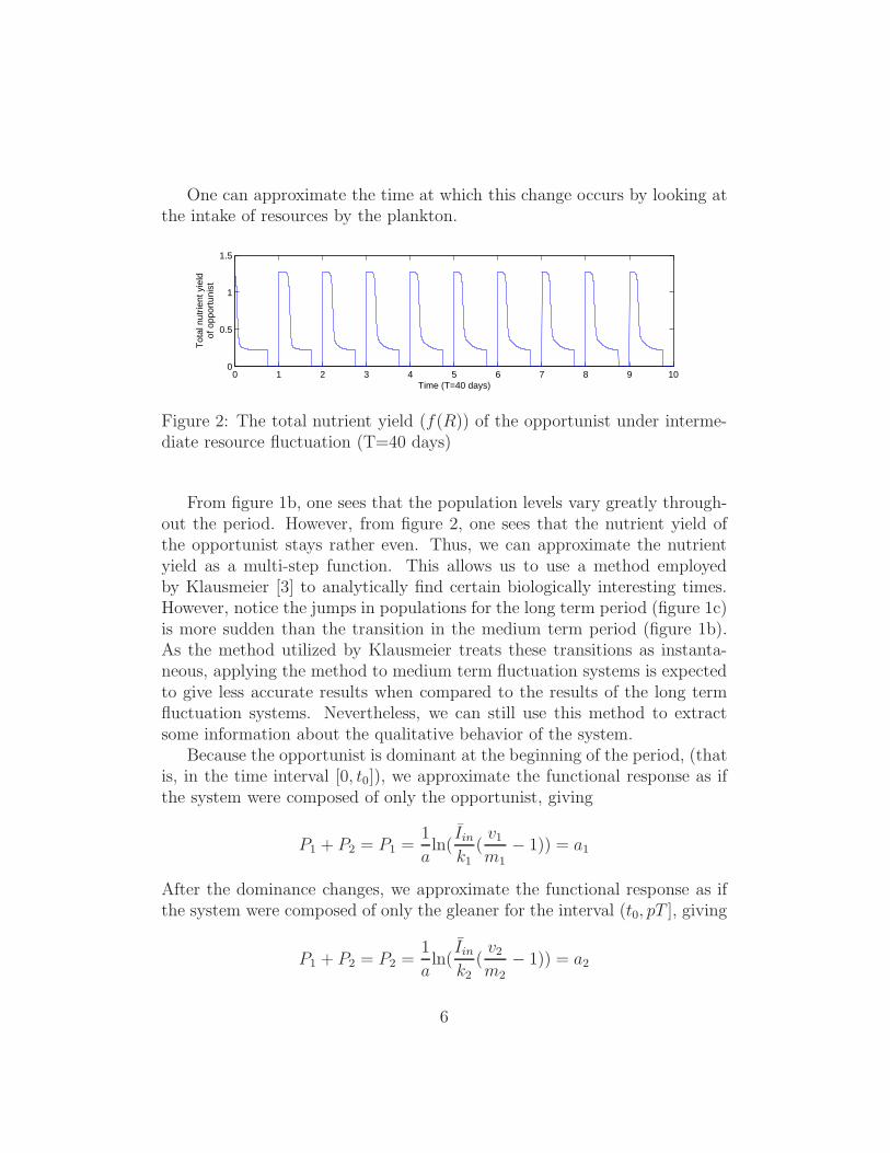
One can approximate the time at which this change occurs by looking atthe intake of resources by the plankton.

0 1 2 3 4 5 6 7 8 9 100

0.5

1

1.5

Time (T=40 days)

Tot

al n

utrie

nt y

ield

of o

ppor

tuni

st

Figure 2: The total nutrient yield (f(R)) of the opportunist under interme-diate resource fluctuation (T=40 days)

From figure 1b, one sees that the population levels vary greatly through-out the period. However, from figure 2, one sees that the nutrient yield ofthe opportunist stays rather even. Thus, we can approximate the nutrientyield as a multi-step function. This allows us to use a method employedby Klausmeier [3] to analytically find certain biologically interesting times.However, notice the jumps in populations for the long term period (figure 1c)is more sudden than the transition in the medium term period (figure 1b).As the method utilized by Klausmeier treats these transitions as instanta-neous, applying the method to medium term fluctuation systems is expectedto give less accurate results when compared to the results of the long termfluctuation systems. Nevertheless, we can still use this method to extractsome information about the qualitative behavior of the system.

Because the opportunist is dominant at the beginning of the period, (thatis, in the time interval [0, t0]), we approximate the functional response as ifthe system were composed of only the opportunist, giving

P1 + P2 = P1 =1

aln(

Iin

k1(

v1

m1− 1)) = a1

After the dominance changes, we approximate the functional response as ifthe system were composed of only the gleaner for the interval (t0, pT ], giving

P1 + P2 = P2 =1

aln(

Iin

k2(

v2

m2− 1)) = a2

6

During the interval (pT, T ), Iin ≡ 0. All this depends on our initial assump-tion of treating the plankton populations as discrete multi-step function. Asthe per capita growth (Pi/Pi) of each plankton over a cycle averages to 0, wehave the following equation

∫ t0

0

f1(Iinea1) − mp1

dt +

∫ pT

t0

f1(Iinea2) − mp1

dt +

∫ T

pT

−mp1dt = 0 (5)

Solving for t0 yields

t0 =T (pf1(Iine

a2) − mp1)

f1(Iinea1) − f1(Iinea2)(6)

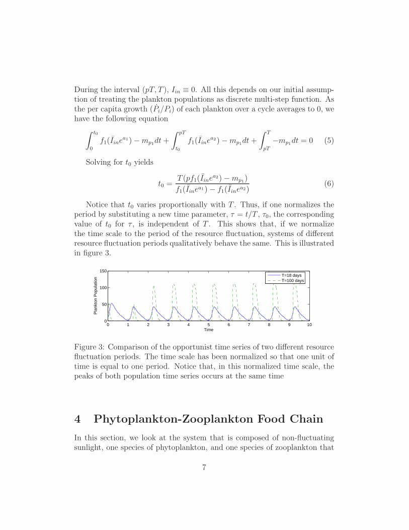
Notice that t0 varies proportionally with T . Thus, if one normalizes theperiod by substituting a new time parameter, τ = t/T , τ0, the correspondingvalue of t0 for τ , is independent of T . This shows that, if we normalizethe time scale to the period of the resource fluctuation, systems of differentresource fluctuation periods qualitatively behave the same. This is illustratedin figure 3.

0 1 2 3 4 5 6 7 8 9 100

50

100

150

Time

Pla

nkto

n P

opul

atio

n

T=18 daysT=100 days

Figure 3: Comparison of the opportunist time series of two different resourcefluctuation periods. The time scale has been normalized so that one unit oftime is equal to one period. Notice that, in this normalized time scale, thepeaks of both population time series occurs at the same time

4 Phytoplankton-Zooplankton Food Chain

In this section, we look at the system that is composed of non-fluctuatingsunlight, one species of phytoplankton, and one species of zooplankton that

7

feeds on the phytoplankton.

P = A(P, Z) = cpg(R)P − mpP,

Z = B(P, Z) = czh(P )Z − mzZ,

R = Iine−aP (7)

Without resource fluctuations, this system has three equilibrium points.One is the trivial equilibrium where both species die out. Another occurswhen the system collapses into the phytoplankton growth model as the zoo-plankton die out. The last and most interesting equilibrium is when thereis coexistence of zooplankton and phytoplankton. By setting Z equal to0, one finds that the nontrivial equilibrium population for phytoplankton isP = −kzmz

vz+mz. The equilibrium populations are

(0, 0), (P , 0), (P ,P + kp

vp

(mp −vpIine

aP

IineaP + kp

))

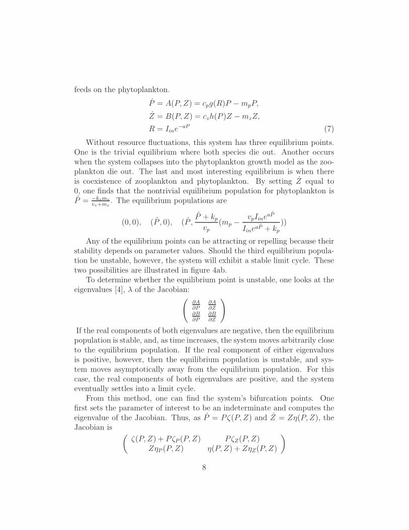
Any of the equilibrium points can be attracting or repelling because theirstability depends on parameter values. Should the third equilibrium popula-tion be unstable, however, the system will exhibit a stable limit cycle. Thesetwo possibilities are illustrated in figure 4ab.

To determine whether the equilibrium point is unstable, one looks at theeigenvalues [4], λ of the Jacobian:

(

∂A∂P

∂A∂Z

∂B∂P

∂B∂Z

)

If the real components of both eigenvalues are negative, then the equilibriumpopulation is stable, and, as time increases, the system moves arbitrarily closeto the equilibrium population. If the real component of either eigenvaluesis positive, however, then the equilibrium population is unstable, and sys-tem moves asymptotically away from the equilibrium population. For thiscase, the real components of both eigenvalues are positive, and the systemeventually settles into a limit cycle.

From this method, one can find the system’s bifurcation points. Onefirst sets the parameter of interest to be an indeterminate and computes theeigenvalue of the Jacobian. Thus, as P = Pζ(P, Z) and Z = Zη(P, Z), theJacobian is

(

ζ(P, Z) + PζP (P, Z) PζZ(P, Z)ZηP (P, Z) η(P, Z) + ZηZ(P, Z)

)

8

0 2 4 6 8 100

20

40

60

80

100

120

Time (T=18 days)

Pla

nkto

n po

pula

tion

PhytoplanktonZooplankton

0 2 4 6 8 105

10

15

20

25

30

35

40

Time (T=18 days)

Pla

nkto

n po

pula

tion

PhytoplanktonZooplankton

(a) (b)

Figure 4: Plankton times series under resource fluctuation. In (a), a = 0.04.In (b), a = 0.1. In (a), one sees a limit cycle. In (b), one sees that bothpopulations asymptotically approach equilibrium.

This matrix has eigenvalues

1

2(ζ + η + 2ζPP ±

√

ζ2 − 2ζη + η2 + 4ζP ζZPZ) (8)

Then one can simply set the real components of both eigenvalues to 0 (makingsure that one does not get a double root) and solve for the indeterminate tofind the bifurcation point.

A system’s normal form is the simplest form the system takes underlinear transformations. By finding it, we can approximate the chain modelfor parameter values close to the bifurcation point. To find the normal form,one first transforms the matrix of the linear terms into an antisymmetricmatrix. Then one applies another transformation that turns the variablesinto complex variables. This gives us two equations, one of which is thecomplex conjugate of the other. Thus, we need only look at one. From this,we apply one final transformation that turns the complex equation into asystem of polar equations. The normal form is derived in the appendix. Theprocess transforms equation 7 to the following equation:

r = αr + ar3 + ...,

θ = ω + br2 + ... (9)

9

Here α and ω are coefficients that appear after all the transformations areapplied.

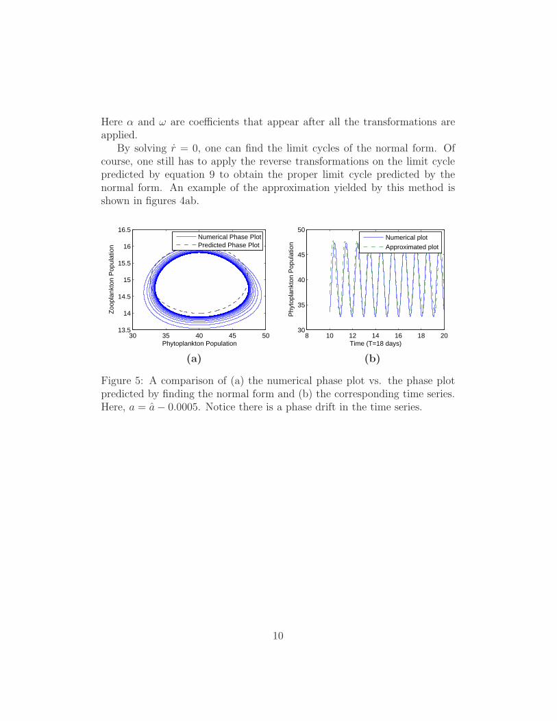
By solving r = 0, one can find the limit cycles of the normal form. Ofcourse, one still has to apply the reverse transformations on the limit cyclepredicted by equation 9 to obtain the proper limit cycle predicted by thenormal form. An example of the approximation yielded by this method isshown in figures 4ab.

30 35 40 45 5013.5

14

14.5

15

15.5

16

16.5

Phytoplankton Population

Zoo

plan

kton

Pop

ulat

ion

Numerical Phase PlotPredicted Phase Plot

8 10 12 14 16 18 2030

35

40

45

50

Time (T=18 days)

Phy

topl

ankt

on P

opul

atio

n

Numerical plot

Approximated plot

(a) (b)

Figure 5: A comparison of (a) the numerical phase plot vs. the phase plotpredicted by finding the normal form and (b) the corresponding time series.Here, a = a − 0.0005. Notice there is a phase drift in the time series.

10

5 Discussion

Certain plankton population models can be simplified (whether it’s by ap-proximations or transformations) while still retaining many of the same qual-itative features. This allows us to study the simplified versions of the systemsto extract information about the original systems.

For the competition model, the analytical methods reveal that, even formedium term fluctuations, one can predict biologically interesting times byusing rough approximations. For this project, we found the time at which theplankton populations change dominance. We accomplished this by extendingKlausmeier’s method to medium term fluctuations by making the assump-tion that, even though the plankton populations were smoothly changing,we could still view them as multi-step functions. This method also showedthat systems of different fluctuation periods can still behave the same, qual-itatively. Thus, when the time scale is normalized, the times at which bio-logically interesting events occur are independent of the period.

We found the bifurcation points of the system with respect to a chosenparameter. Using normal forms, one can approximate the phase plot of thesystem around the equilibrium point. From this, one can also approximatethe behavior of the system near the coexistence equilibrium. However, ifone goes too far away from the bifurcation point, the approximation breaksdown.

Notice that none of the conditions used restricted our analysis exclusivelyto plankton. Thus, as long as our assumptions (well-mixing, no intra-trophicrelations, etc.) are applicable to an organism of interest, our analytical tech-niques may be used to study its food web.

6 Acknowledgements

I would like to thank Caltech’s SURF program for providing me the resourcesto do research. I would like to thank my SURF mentor Mason Porter for hisinvaluable help and support (and additional resources). I would like to thankJulie Bjornstad and Alexei Dachevski for providing guidance. I would alsolike to thank Christopher Klausmeier for providing feedback from a biologist’spoint of view.

11

A Appendix

To find a bifurcation’s normal form, one first shifts the system so that theequilibrium point is at the origin and the bifurcation point occurs when theparameter of interest, µ, has a value of 0 [5]. This can be achieve by makingthe substitutions: x = P−P , y = Z−Z, and ǫ = µ−µ, where the bifurcationof equilibrium (P , Z) occurs at parameter value, µ.

Then one tries to reduce the number of variables in the systems. Thiscan be accomplished by introducing complex variables. One first has toapply the linear transformation, (x1, y1)

T = S1S−12 (x, y)T , where S1 is the

eigenvector matrix of the linearized system and S2 is the eigenvector matrixof the antisymmetric matrix:

(

Re(λ) −Im(λ)Im(λ) Re(λ)

)

This turns the system into the form:(

x1

y1

)

=

(

Re(λ) −Im(λ)Im(λ) Re(λ)

)(

x1

y1

)

+

(

f1(x1, y1; ǫ)f2(x1, y1; ǫ)

)

(10)

Here, f1 and f2 are the higher order, nonlinear components of the equations.One then transforms to the complex variables, setting (z, z) = (x1 + iy1, x1−iy1) to obtain:

(

z˙z

)

= |λ|

(

e2πiθ 00 e−2πiθ

)(

zz

)

+

(

g1(z, z; ǫ)g2(z, z; ǫ)

)

(11)

One can verify that g1 and g2 are complex conjugate functions. Thus, as theabove system contains two complex conjugate equations, we only needs tolook at one, giving us the equation: z = |λ|e2πiθz + g1(z, z; ǫ). As discussedin Wiggins [5], when expanding g1 out to four terms, only the z2z cannot beeliminated for ǫ sufficiently small. This gives us the equation:

z = |λ|e2πiθz + cz2z + O(5) (12)

where O(5) denotes all terms with combined exponent greater than or equalto 5. Expressing the coefficients as complex numbers gives |λ|e2πiθ = α + iωand c = a + ib. By grouping like terms, one gets the following system:

x = αx − ωy + (ax − by)(x2 + y2) + O(5),

y = ωx + αy + (bx + ay)(x2 + y2) + O(5) (13)

12

Equation 13, in polar coordinates, can be expressed as

r = αr + ar3 + ...,

θ = ω + br2 + ... (14)

13

References

[1] G. Evelyn Hutchinson. The Paradox of the Plankton. The American

Naturalist, 95:137–145, 1961.

[2] Winfried Lampert and Ulrich Sommer. Limnoecology: The Ecology of

Lakes and Streams. Oxford University Press, 1997.

[3] Elena Litchman and Christopher A. Klausmeier. Competition of Phy-toplankton under Fluctuating Light. The American Naturalist, 157:170–187, 2001.

[4] Stephen H. Strogatz. Nonlinear Dynamics and Chaos. Westview Press,1994.

[5] Stephen Wiggins. Introduction to Applied Nonlinear Dynamical Systems

and Chaos. Springer, 1990.

14