Analysis of Sentinel-1 SAR data for mapping standing water

Analysis of Sentinel-1 SAR data

for mapping standing water in

the Twente region

CHANG LIU

February, 2016

SUPERVISORS:

Dr. Ir. Rogier van der Velde

Dr. Zoltá n Vekerdy

Thesis submitted to the Faculty of Geo-Information Science and Earth

Observation of the University of Twente in partial fulfilment of the

requirements for the degree of Master of Science in Geo-information Science

and Earth Observation.

Specialization: Water Resource and Environmental Management

SUPERVISORS:

Dr. Ir. Rogier van der Velde

Dr. Zoltá n Vekerdy

THESIS ASSESSMENT BOARD:

Dr. Ir. C. van der Tol (Chair)

Dr .Tao Wang (External Examiner, Capital Normal Unviversity)

Analysis of Sentinel-1 SAR data

for mapping standing water in the

Twente region

CHANG LIU

Enschede, The Netherlands, February, 2016

DISCLAIMER

This document describes work undertaken as part of a programme of study at the Faculty of Geo-Information Science and

Earth Observation of the University of Twente. All views and opinions expressed therein remain the sole responsibility of the

author, and do not necessarily represent those of the Faculty.

i

ABSTRACT

The Sentinel-1 mission is expected to deliver a wealth of data and imagery. As the first member of the

constellation of two satellites, the Sentinel-1A with C-band was launched on 3rd

April, 2014. It has

dual-polarization capability (HH+HV or VV+VH) which can provide more ground surface

information. This study aims to analyse Sentinel-1 SAR data for its potential to map standing water in

agricultural fields over the Twente region.

Level-1 Ground Range Detected (GRD) Sentinel-1 C-band (5.405 GHz) data collected in the

Interferometric Wide swath (IW) mode were used to develop a procedure for reliable processing of the

Sentinel-1 SAR images. There are 73 SAR images have been collected during the period from October

2014 to September, 2015. Those series SAR images were utilized to investigate the multi-temporal

backscatter properties (e.g. mean and standard deviation) for different land cover across the Twente

region. Based on the backscatter temporal variability, multi-temporal backscatter observations can be

used to classify the agricultural field from forest, urban, open water body and grassland. However,

because of the effect of surface roughness, soil moisture and vegetation growth, winter wheat and corn

field are difficult to distinguish.

Fieldwork has been done from 17th September, 2015 to 2

nd October, 2015 to find the standing water in

agricultural fields. At the same time, the landscape changes and agricultural activities were also

recorded in order to analyse backscatter changes with respect to human activities. There are 6 fields

had been visited including two grassland, two corn fields and two winter wheat fields. Only one winter

wheat fields (No.7 field) had obvious surface water. Standing water in one grassland (No.4 field)

spread as mosaic under the thick grass.

In addition, backscatter changes in response to atmospheric forcings (e.g. rainfall) and land surface

conditions (e.g. soil moisture) were analyzed for the individual fields with different land covers (e.g.

grassland, winter wheat, corn) to find the possible periodically standing water. Among all the possible

influence factors, soil moisture is the dominant factors in backscatter changes. However, standing

water is difficult to delineate from the Sentnel-1 images due to the uncertainties. Those uncertainties

include different surface conditions in each agricultural field, soil moisture, vegetation characteristics

and agricultural activities. Those factors vary from temporal and spatial scale, like farming practices

and atmospheric forcings.

Keywords: Standing water, Agricultural fields, Sentinel-1, Backscatter analysis

.

ii

ACKNOWLEDGEMENTS

First and foremost, I must show my very profound gratitude to my parents for their support and always

encourage me to do my studies.

Then I would like to express my sincere thanks to my first supervisor Dr.Rogier van der Velde for his

advices, suggestions, continuous guidance throughout the thesis work and even guide in my thesis

writing. I would also like to thank my second supervisor Dr. Zoltan Vekerdy for his precious time,

new thoughts, advices, guidance and comments to improve the thesis.

I would also like to thank my teacher Mrs. Wang (Lichun Wang) for helping me with IDL coding, and

Phd student H.F. Benninga for helping me solve the problems during my thesis work.

Finally, I would like to say big thank you to my friends for supporting and encouraging me to finish

my study, researching and writing this thesis. Thank you.

.

iii

TABLE OF CONTENTS

1. Introduction ......................................................................................................................................1

1.1. Background .......................................................................................................................................... 1

1.2. Open water detection using SAR ......................................................................................................... 2

1.2.1. Overview of spaceborne SAR Sensors ...................................................................................2

1.2.2. Detection of open water .........................................................................................................2

1.3. Research problem ................................................................................................................................ 3

1.4. Objectives and research questions ....................................................................................................... 4

1.4.1. General objective ....................................................................................................................4

1.4.2. Specific objectives ..................................................................................................................4

1.4.3. Research questions .................................................................................................................4

1.5. Thesis and research structure ............................................................................................................... 4

2. Study area and data ...........................................................................................................................6

2.1. Study area ............................................................................................................................................ 6

2.2. Sentinel-1 data ..................................................................................................................................... 6

2.3. Rainfall data ......................................................................................................................................... 7

2.4. Soil moisture data ................................................................................................................................ 7

2.5. Vegetation index .................................................................................................................................. 8

2.6. Land cover data .................................................................................................................................... 8

3. Methodology ...................................................................................................................................11

3.1. Fieldwork ........................................................................................................................................... 11

3.2. Identification of agricultural areas ..................................................................................................... 11

3.3. Standing water detection and verification .......................................................................................... 13

4. Fieldwork ........................................................................................................................................14

4.1. Description of the observed fields ..................................................................................................... 14

4.2. Landscape changes during the fieldwork ........................................................................................... 14

5. Sentinel-1 data Pre-processing .......................................................................................................18

5.1. Terrain correction .............................................................................................................................. 18

5.2. View angle review ............................................................................................................................. 19

5.3. Speckle filter ...................................................................................................................................... 19

6. Backscatter analysis ........................................................................................................................22

6.1. Image based backscatter analysis ....................................................................................................... 22

6.2. Field-scale backscatter changes and standing water detection ........................................................... 25

6.3. Temporal verification......................................................................................................................... 27

6.3.1. Rainfall and soil moisture trend ...........................................................................................27

6.3.2. NDVI for agricultural fields .................................................................................................28

6.3.3. Periodically standing water in winter wheat field ................................................................29

6.3.4. Periodically standing water in grassland ..............................................................................30

7. Conclusion and recommendation ...................................................................................................32

7.1. Conclusions ........................................................................................................................................ 32

7.2. Limitations and recommendations ..................................................................................................... 32

iv

LIST OF FIGURES

Figure 1 Flowchart of research method ......................................................................................................... 5

Figure 2 On the left: map of Netherlands with the Twente region highlighted. On the right:

Google Earth image of the area covered by the soil moisture stations and weather monitoring

stations belong to the Royal Netherlands Meteorological Institute (KNMI). .............................. 6

Figure 3 Daily rainfall from 2010 to 2014 in Twente KNMI monitoring station as highlight in

Figure 1 ........................................................................................................................................................ 7

Figure 4 Vegetation Index (NDVI) for observed fields provided by Groenmonitor website

(http://www.groenmonitor.nl/groenindex) ........................................................................................... 8

Figure 5 Land cover map of study area available on the websit of Overijssel by the Province of

Overijssel (http://gisopenbaar.overijssel.nl/viewer/app/bodematlas/v1) ....................................... 9

Figure 6 Scattering mechanisms (http://imaging.geocomm.com/faq/) ................................................. 11

Figure 7 The distribution of land cover classes in the backscatter temporal variability and long-

term coherence feature space (Bruzzone et al., 2004). .................................................................... 12

Figure 8 Landscape in each observation field. ........................................................................................... 14

Figure 9 Sentinel-1data processing steps ..................................................................................................... 18

Figure 10 Filter results of VH-polarized SAR images acquired on 16-09-2015 ................................ 20

Figure 11 Backscatter (in dB) for RGB colour composite (Green--VH polarization; Red and Blue-

-VV polarization) at different dates. .................................................................................................... 21

Figure 12 Backscatter temporal variability calculated by different estimators for RGB colour

composite (Green--VH polarization; Red and Blue--VV polarization) at different dates : (a)

Saturation backscatter; (b) Maximum-Minimum Ratio in dB; (c) Logarithmic measure

based on normalized Standard deviation; (d) Normalized standard devition ............................. 22

Figure 13 Backscatter statistics result for RGB colour composite (Green--VH polarization; Red

and Blue--VV polarization): (a) mean backscatter (in dB); (b) standard deviation of

backscatter (in dB) ................................................................................................................................... 23

Figure 14 Backscatter statistics for different land cover classes, (a) Standard deviation for VH and

VV polarization, (b) Average backscatter for VH and VV polarization. .................................... 25

Figure 15 Backscatter changes of different land cover ............................................................................ 26

Figure 16 Daily rainfall data collected from Twente station, and the soil moisture data averaged

from the 20 soil moisture network stations in Tewnte from October 2014 to September 2015.

...................................................................................................................................................................... 27

Figure 17 NDVI for corn fields, winter wheat field and grassland. ...................................................... 29

Figure 18 Soil moisture with backscatter of No.9 field and daily rainfall derived from Twente

station. ........................................................................................................................................................ 30

Figure 19 Soil moisture with backscatter [dB] of No.4 field and daily rainfall derived from

Twente station .......................................................................................................................................... 31

v

LIST OF TABLES

Table 1 Characteristics of the Sentinel-1 Interferometric Wide swath mode nominal measurement

modes (Torres et al., 2012; Sentinel-1 Team, 2013). ......................................................................... 7

Table 2 Backscatter estimators ...................................................................................................................... 12

Table 3 Landscape changes in No.7 observed fields................................................................................ 15



Table 6 Dynamic range of backscatter in different land cover .............................................................. 25

ANALYSIS OF SENTINEL-1 SAR DATA FOR MAPPING STANDING WATER IN THE TWENTE REGION

1

1. INTRODUCTION

1.1. Background

Standing water occurs as a result of heavy or persistent rainfall, flooding by rivers and lakes, water

table rise, snowmelt above frozen soils, or artificially as a result of the construction of reservoirs.

Standing water on agricultural fields is likely to influence the crop growth conditions, lead to poor soil

aeration, increases the pH of acid soils and decreases the pH of alkaline soils. When standing water

occurs, some degree of damage to the crop is usually inevitable. The extent of the damage depends on

the crop type, its growth stage, the duration of standing water, and temperatures during standing water.

Damage occurs because water logged soils are quickly depleted of oxygen in the root zone, and the

supply of oxygen to water logged soil is severely limited. Most crops require oxygen for normal

metabolism, growth and development. Furthermore, standing water frequently results in higher levels

of plant diseases that reduce yields. Berning et al. (2000) showed that the depth and duration of

standing water were two dominant factors leading to the decrease of sugar-cane harvest in the Mfolozi

floodplain. Furthermore, due to the fact that the soil is moist and soft under the conditions of standing

water, many agricultural activities with respect to ploughing, seeding, and harvesting can be also

affected.

In recent years, space-borne remote sensing has widely been recognized as a technique that is

beneficial for quantitative estimation of flooded extent. Remote sensing images from optical, thermal,

and microwave wavelengths can be used for standing water delineation. However, the major challenge

in the application of visible or thermal imagery to standing water mapping is that flood events are

often associated with cloud cover, particularly in the small and medium-size areas (Ticehurst et al.,

2009; Schlaffer et al., 2015). Moreover, vegetation canopies also limit the applicability of these

sensors to map standing water extent. Water cannot be detected when the surface ponding is in the

shadow of the vegetation cover. On the other hand, optical imagery is easy to interpret, and the

extraction of the standing water area from optical imagery is generally more straightforward than from

radar imagery (Schumann et al., 2009). Compared with optical sensors, microwaves sensors have

longer wavelengths varying from less than one centimeter to one meter (or frequencies from 89 GHz

to 0.3 GHz) (Ticehurst et al., 2009). Synthetic Aperture Radar (SAR) is an active microwave remote

sensing technique with the capability of being independent of solar illumination. Due to the

wavelength, the signal has limited interaction with the droplets in the cloud without obscuring

observations (G. Schumann et al., 2009). More importantly, because of SAR systems are capable of

acquiring observations in both day-time and night-time and even under extreme weather conditions, it

becomes the most suitable instruments for high-resolution flood mapping from space (Hostache et al.,

2012). In general, the return signals of SAR are influenced by the view angle of the sensor, the

material of the reflecting objects and the surface roughness as well as the frequency and polarization

(Gstaiger et al., 2012; Townsend & Walsh, 1998). Nowadays more and more microwave satellites are

available with high resolution, such as TerraSAR-X, COSMO-SkyMed, RADARSAT-2 and Sentinel-

1. Also for given the rapid flood recession in small to medium sized catchments, the delineation of

standing water extent and systematic monitoring seems realistically more feasible with SAR imagery

(G. J.-P. Schumann & Moller, 2015).


2

1.2. Open water detection using SAR

In this section, satellites for detecting flood extent and methods for delineating flood area are reviewed.

1.2.1. Overview of spaceborne SAR Sensors

Since the launch of the first radar satellite SEASAT, in 1978, microwave sensors have increasingly

been used for flood delineation. The two European Remote Sensing Satellites, ERS-1, and ERS-2 were

launched in 1991 and 1995, respectively. These two ESA satellites were in charge of collecting a

wealth of valuable data associated with land surface, ocean, polar caps, and natural disasters (ERS

overview). The Advanced Synthetic Aperture Radar (ASAR) on the ENVISAT satellite is an improved

version of the sensors on ERS by offering five polarization configurations: HH, VV, HH/VV, HV/HH,

VH/VV (Henry et al., 2006). In addition, it enhances the capabilities in terms of coverage, range of

incidence angles, polarisation, and modes of operation (ASAR - Earth Online). With a moderate

resolution of 30 m, ENVISAT has been used for extracting the standing water extent in rural areas

( Kuenzer et al., 2013; Matgen et al., 2011). Unfortunately, the ENVISAT mission ended on 8th April,

2012 following from the unexpected loss of contact with the satellite. More recently, a number of SAR

sensors with high resolution as fine as 3 m or higher are available for both urban and rural flood

mapping studies, such as RADARSAT-2 (C-band), TerraSar-X (X-band), and four COSMO-SkyMed

(X-band) satellites ( Gstaiger et al., 2012; Pulvirenti et al., 2011). Compared to those high resolution

sensors, Sentinel-1 has the higher temporal resolution due to its configuration: two satellites work at

the same time increasing the re-visit time to maximum 5 days. Moreover, Sentinel-1 can cover large

areas and the images are free to the public. Gstaiger et al.(2012) showed that TerraSAR-X data could

provide water mask with very high spatial detail and accuracy, but covers only small areas depending

on the acquisition mode.

The Sentinel-1 mission is expected to deliver a wealth of data and imagery that are central to the

Copernicus joint initiative of the European Commission (EC) and European Space Agency (ESA). As

the first member of the constellation of two satellites, the Sentinel-1A was launched on 3rd

April, 2014

with a revisit cycle of 12 days. Sentinel-1 includes C-band imaging Synthetic Aperture Radar (SAR) in

four exclusive imaging modes: Interferometric Wide Swath Mode (IW), Wave-Mode (WM), Strip

Map Mode (SM), and Extra-Wide Swath Mode (EW). With different resolutions (from 5 m to 40 m)

and coverage (from 80 km to 400 km), the four modes can meet the demanding image quality and

swath width requirements (Sentinel-1 User handbook, 2013).

1.2.2. Detection of open water

The features of standing water or surface conditions in SAR imagery are the result of different factors,

including acquisition characteristics (wavelength, incidence angle, polarization), soil moisture,

vegetation characteristics, and soil surface conditions (roughness and inundation) (Hostache et al.,

2012). For transmission/acquisition characteristics, polarization refers to the direction of the electric

field vector of the transmitted/received beam with respect to the horizontal direction. Sentinel-1

provides selectable polarization capability: selectable single polarization (VV or HH) for Wave-Mode

and selectable dual-polarization (VV+VH or HH+HV) for the other three modes (Attema et al., 2009).

Previous studies conclude that the dual-polarization data HH + HV gave the most informative result

for flood mapping (Matgen et al., 2011). As an alternative, the single polarization model HH can also

be used for flood mapping, better than VV, or cross-polarized used individually, without HH, since the

HH-polarized data is less influenced by suface roughness on open water caused by waves (Henry et al.,

2006).

During the last decade, many methods have been developed for flood mapping with SAR images.

From a general perspective, these methods can be divided into two categories: single-image analysis


3

and change detection approaches (Schlaffer et al., 2015). Single-image analysis is performed without

considering how surface ponding changes over time. Schumann et al. (2009) investigated the use of

several single-image analysis methods, like visual interpretation, image texture analysis, histogram

thresholding, and edge detection approach. The authors concluded that flood mapping with a multi-

algorithm including visual interpretation, image texture analysis, histogram thresholding, and edge

detection approach integrated method, gave better result than using only a single algorithm. Similar

results can be found in the work by Di Baldassarre et al., (2009b), who used the aforementioned four

methods together with an Euclidean distance method to get inundation maps derived from both coarse

resolution (150 m) images (ENVISAT ASAR WS) and high resolution (12.5 m) satellite images (ERS-

2 SAR). Their results demonstrated that visual interpretation and image texture analysis were largely

rely on the sensitivity of feature differences in the human visual system. Hence, interpreting the flood

boundary visually depends much on the operator’s ability of distinguishing different grey scale tones

and their knowledge of the flood process. In another study, a thresholding technique has been viewed

as an efficient flood mapping method (Schumann et al., 2009). In general, thresholding is a key point

in the histogram-based approach and pattern recognition (Bazi et al., 2007). Gstaiger et al.,(2012)

compared three simple approaches to derive standing water areas from TerraSAR-X data. Two

methods are pixel-based and use histogram-based empirically defined grey-level thresholds, as well as

a homogeneity criterion for classification. The third approach is object-based by using empirically

chosen values and thresholds for classification with several segments attributes, such as grey value,

shape, texture and relations to neighbouring objects (Gstaiger et al., 2012). Those attributes were

analysed and taken into consideration in a decision tree to classify water and non-water areas. Kuenzer

et al. (2013) employed 60 ENVISAT ASAR Wide Swath mode images with simple, empirically

chosen thresholds to understand the flood inundation pattern in the Mekong Delta during 2007-2011.

Furthermore, hybrid methods have been proposed by combining thresholding algorithms with other

image analysis approaches, e.g. region growing method (Giustarini et al., 2013; Matgen et al., 2011).

From their studies, a threshold was used to extract the core of the water bodies from SAR data and to

identify the seed region for the region growing step. Then neighbouring pixels were identified which

have similar backscatter values to those in the seed region. Moreover, a fuzzy logic was used to

improve the accuracy of flood mapping by taking into account ancillary hydraulic characteristic and

contextual information (Pulvirenti et al. 2011). In order to separate the permanent and the temporarily

flooded areas and to overcome the disadvantages of single-image analysis methods, much attention has

been devoted to integrating change detection approaches to the aforementioned single-image analysis

methods.

1.3. Research problem

Due to the fact that in the summer the potential evapotranspiration (ETp) is higher than the

precipitation, but in the winter the precipitation exceeds the ETp, the surface and subsurface runoff,

standing water events occur at agricultural fields. As the previous studies introduced in Section 1.2, the

potential of mapping the extent of inundation in floodplains using satellite images is widely

acknowledged. However, various problems are involved in standing water mapping with satellite

remote sensing imagery at field scale. For instance, standing water on agricultural fields is patchy,

leading to the mixing of signals from land and open water both at the optical and the radar

wavelengths. Also, the presence of vegetation can obscure observation of surface ponding in fields.

Furthermore, due to the agricultural seasonality, the standing water situation is different on fields with

different crop within one image. These features add uncertainty to the standing water mapping.


4

1.4. Objectives and research questions

1.4.1. General objective

This study aims to analyse Sentinel-1 SAR data for its potential to map standing water in agricultural

fields over the Twente region.

1.4.2. Specific objectives

In order to achieve the general objective of this research three specific objectives are formulated as

follows.

1) To develop a procedure for reliable processing of the Sentinel-1 SAR images;

2) To investigate the multi-temporal backscatter properties (e.g. mean and standard deviation) for

different land cover across the Twente region;

3) To analyse the backscatter changes for the individual fields with different land covers (e.g.

grassland, winter wheat, corn) in response to atmospheric forcings (e.g. rainfall) and land surface

conditions (e.g. soil moisture).

1.4.3. Research questions

The questions related to the aforementioned sub-objectives are illustrated as follows.

Can the raw Sentinel-1 data be processed to reliable SAR imagery?

How do the multi-temperoral Sentine-1 backscatter properties (e.g. mean and standard deviation) vary

with land cover?

Can standing water within agricultural field be detected from a series of Sentinel-1 images?

1.5. Thesis and research structure

This thesis is organized in seven chapters. Study area and main dataset, like Sentinel-1 SAR images

and ancillary dataset are introduced in Chapter 2. Chapter 3 descrips the methodology, which is used

to analyze Sentinel-1 SAR data for its potential to map standing water within agricultural fields.

Chapter 4 present the fieldwork observation and landscape. In Chapter 5, Sentinel-1 images pre-

processing steps and results are descrbed in details. Chapter 6 contains the backscatter analysis with

respect to image-based backscatter analysis and field-scale backscatter change. Based on those

analysis, possible periodically standing water will be dectecd from the backscatter changes throughout

the study period. In addition, ancillary data like in-situ rainfall, soil moisture and NDVI are usde to

verify the possible standing water. Finally, in Chapter 7, conclusion and recommendation are drawn.

An overview of the research method is showed in Figure 1.


5

Figure 1 Flowchart of research method

Analyse the potential to

map standing water

Sentinel-1 images

Standing water

detection

Terrain Correction

Backscatter Analysis

(Image & Field based)

Fieldwprk

View angel correction

Speckle filter

Soil moisture

Verification

Rainfall

NDVI

Shift the images


6

2. STUDY AREA AND DATA

2.1. Study area

The study area is located in the Twente region in the eastern part of Overijssel province (eastern

Netherlands). The study area is between longitudes 6.6°- 7.1 °E and latitudes 52.1°- 51.5 °, including

the city of Enschede as shown in Figure 2. The terrain of the study area is flat, with an elevation

ranging between 1 m to 83 m above mean sea level. The land cover of this area includes a mosaic of

agricultural fields (winter wheat, corn fields and grassland), forest patches and several urban areas

(Dente et al., 2012). The average temperature in Enschede is 9.1 °C and the average annual rainfall is

782 mm. Monthly precipitation amounts are evenly spread over the year. Monthly precipitation from

1974 to 2009 is around 70 mm (Dente et al., 2011).

Figure 2 On the left: map of Netherlands with the Twente region highlighted. On the right: Google Earth image

of the area covered by the soil moisture stations and weather monitoring stations belong to the Royal

Netherlands Meteorological Institute (KNMI).

2.2. Sentinel-1 data

In this research, Level-1 Ground Range Detected (GRD) Sentinel-1 C-band (5.405 GHz) data

collected in the Interferometric Wide swath (IW) mode were used. This mode allows the combination

of a large swath width (250 km) with a moderate geometric resolution (10 m). Moreover, it has dual-

polarization capability (HH+HV or VV+VH) which can provide more ground surface information. 73

SAR images have been used for the period from October 2014 to September, 2015, which are freely

available from the European Space Agency (ESA) through Sentinels Scientific Data Hub

(https://scihub.esa.int/dhus/). The time interval of the acquired images varies from 2 days up to 11

days. The main characteristics of the collected Sentinel -1 IW data are provided in Table 1 (Torres et

al., 2012). The IW mode is the default acquisition mode over land.

https://scihub.esa.int/dhus/


7

Table 1 Characteristics of the Sentinel-1 Interferometric Wide swath mode nominal measurement modes (Torres

et al., 2012; Sentinel-1 Team, 2013).

Parameter Interferometric Wide-swath mode(IW)

Swath width 250 km

Incidence angle range 29.1° - 46.0°

Sub-swaths 3

Azmiuth steering angle ± 0.6°

Azmiuth and range looks Single

Polarisation options Dual VV+VH

Maximum Noise Equivalent Sigma Zero (NESZ) -22 dB

Radiometric stability 0.5 dB (3σ)

Pixel size (meter) 10

2.3. Rainfall data

The daily rainfall data are available from the Royal Netherlands Meteorological Institute (KNMI,

http://www.knmi.nl/nederland-nu/klimatologie/daggegevens). In this study, daily rainfall data from

October, 2014 to September, 2015 were collected at the Twente station located in the Twente region

near Enschede (Figure 2). As shown in Figure 3, the rainfall is spread over the study period. It is clear

seen that rainfall events concentrated in July and August. The peak of daily rainfall occurs in August

as high as 34.2 mm a day.

Figure 3 Daily rainfall from 2010 to 2014 in Twente KNMI monitoring station as highlight in Figure 1

2.4. Soil moisture data

Soil moisture data are derived from the ITC soil moisture monitoring network (L Dente et al., 2011).

There are 20 stations in the soil moisture monitoring network which are located over eastern part of

the Overijssel province. All the soil moisture sites are marked as yellow points in Figure 2. The 20 soil

moisture stations spread over an area of about 50 km × 40 km large area (52°05’- 52°27’N, 6°05’-

7°00’E). Soil moisture data has been recorded every 15 minutes, while in some field the data is

missing. In each observed field, there is a soil moisture monitoring station. The observed field was

named after the number of soil moisture monitoring station in the same field. During the fieldwork, 5

fields named after the soil moisture sites (No. 3, 4, 7, 8, 9) had been visited. The soil mositure

measurements are collected at both 5 and 10 cm depth. As Sentinel-1 is to provide C-band SAR data,

top layer soil (5 cm) moisture data is used to verify the possible standing water.

0

5

10

15

20

25

30

35

40

20

14

10

01

20

14

10

17

20

14

11

02

20

14

11

18

20

14

12

04

20

14

12

20

20

15

01

05

20

15

01

21

20

15

02

06

20

15

02

22

20

15

03

10

20

15

03

26

20

15

04

11

20

15

04

27

20

15

05

13

20

15

05

29

20

15

06

14

20

15

06

30

20

15

07

16

20

15

08

01

20

15

08

17

20

15

09

02

20

15

09

18

Rai

nfa

ll (m

m)

RainfallDate

http://www.knmi.nl/nederland-nu/klimatologie/daggegevens


8

2.5. Vegetation index

The Normalized Difference Vegetation Index (NDVI) is a numerical indicator for the amount of green

biomass with a value between 0 and 1. It has been widely applied to estimate crop yields, pasture

performance, and rangeland carrying capacities among others. In this study, MODIS NDVI was

utilized first for considering the crop growth stage and agricultural activities. NDVI 16-day interval

product (250 m) composite grid data (MOD13Q1) in HDF format were acquired for the period

between October 2014 and September 2015 (23 images) from the NASA Earth Observing System

(EOS). However, due the observed field is as small as 220 m ×450 m (e.g., No.3 field, the relatively

lager one). The MODIS NDVI product is not good enough to describe the vegetation density at such

small scale. Therefore, vegetation index (NDVI) was derived from Groenmonitor website

(http://www.groenmonitor.nl/groenindex).

Figure 4 Vegetation Index (NDVI) for observed fields provided by Groenmonitor website

(http://www.groenmonitor.nl/groenindex)

2.6. Land cover data

The land cover map is provided by the Atlas of Overijssel by the Province of Overijssel

(http://gisopenbaar.overijssel.nl/viewer/app/bodematlas/v1, Figure 5). The main land covers are

agricultural fields, forest, and buildings. The main crop is corn, which is seeded in April/early May,

and harvested in September/October. Another important seasonal crop is winter wheat. Perennial

grassland are used for pasture or harvested several times a year. In this study, the land cover of

observation fields includes winter wheat, corn and grassland.

http://www.groenmonitor.nl/groenindex

http://www.groenmonitor.nl/groenindex


9

Figure 5 Land cover map of study area available on the websit of Overijssel by the Province of Overijssel

(http://gisopenbaar.overijssel.nl/viewer/app/bodematlas/v1)


11

3. METHODOLOGY

Delineation of standing water from SAR data mainly makes use of the unique characteristics, e.g.

water body exhibit in interaction with microwaves. Calm open water acts as a specular reflector,

scattering the incoming signal reflects away from the sensor (Figure 6 a). Since the sensor receives a

low backscattered signal, water appears dark in the SAR images compared to the backscatter signals

from vegetation or other land surfaces. Compared to water, microwaves incident on a rough surface

are scattered in many directions, which is known as diffuse reflection and result in a brighter tone on

the radar imagery (Figure 6 b). Moreover, backscatter is also affected by the dielectric properties of the

surface. When surface water disappeared shortly after the event of standing water, the soil moisture is

close to saturation. The increase of the soil dielectric constant with water content leads to an enhanced

signal return unless the inundation doesn’t over the area when it rained or the surrounding soils were

already saturated before the flooding (Hostache et al., 2012). Those backscatter changes can be used to

delineate the water logged areas. However, the yearly vegetation cycles may also cause changes of

backscatter, such as volumetric scattering from a tree (Figure 6 c). With volume scattering, radar

sensor may receive backscatter from both the target surface and the interior volume scattering of the

target. Furthermore, some surface objects with respect to dry, bare sand, such as paved highways, may

be easily confused with calm open water bodies due to the similar low backscatter from their surfaces.

a b c

Figure 6 Scattering mechanisms (http://imaging.geocomm.com/faq/)

3.1. Fieldwork

Fieldwork has been done from 17th September, 2015 to 2

nd October, 2015, nearly twice a week and in

total 5 times. The main purpose of the fieldwork is to find the standing water in agricultural fields and

record the outline of the water areas by using GPS. At the same time, the landscape was described in

the observation note. Also the time of landscape changes and agricultural activities were recorded in

order to analyse backscatter changes with respect to human activities.

3.2. Identification of agricultural areas

As the features of standing water in SAR imagery are the results of different factors, mainly including

surface roughness, soil moisture, and vegetation biomass. The characteristics of backscatter are

different for different land cover types or different time period for the same field. Therefore, those

characteristics of backscatter were expected to contribute to identify the land cover type and delineate

the agricultural areas. The cross-polarized information of SAR is known to be sensitive to volume

scattering processes and can be related to the land cover type and structure of vegetation (Cloude,

2009). In this study, backscatter temporal variability was calculated from pixel basis dual-polarized

information for 73 images. Previous studies indicated that vegetated area backscatter variations are

http://imaging.geocomm.com/faq/


12

more stable in densely vegetated, deep-rooted area than in less dense areas, such as grass (Mtamba et

al., 2015). In densely vegetated areas, such as forest, the backscatter response is more or less constant

during all seasons because they can maintain their water content even during the dry season. Previous

literature also showed that the separation between forest and agricultural fields is good based on

temporal variability (Figure 7), mainly due to the higher variability effected by the factors mentioned

above. Urban areas usually with low temporal variability (Bruzzone et al., 2004). In order to better

identify the agricultural areas, the mean backscattering coefficient can be used to increase the

effectiveness of feature set consideration.

Figure 7 The distribution of land cover classes in the backscatter temporal variability and long-term coherence

feature space (Bruzzone et al., 2004).

Previous study showed that high mean backscatter and low standard deviation were observed in

forest/papyrus/thicket vegetation areas(Mtamba et al. 2015). Agricultural fields outside the floodplain

were characterized by low backscatter and high standard deviation. For the above reasons, backscatter

temporal variability estimators relative to the SAR signal feature are used to locate agricultural areas.

The land cover map shown in Figure 5 and Google Earth were used to validate results. The estimation

of temporal variability from the backscatter can be derived according to the following estimators of N

SAR images (Table 2).

Table 2 Backscatter estimators

Estimators Equations

Standard Deviation stdev = √1

N∗ ∑ (σi

2Ni=1 − σave

2 )

Normalized

Standard Deviation

stdev

σave= √

1

N∗ ∑

σi2

σave2

Ni=1 − 1

Logarithmic Measure Based on

Normalized Standard Deviation

10 ∗ log10(stdev

σave

+ 1)

Saturation satuation = σmax− σmin

σmax

Standard Deviation

of dB Values: stdev = √1

N∗ ∑ (10 ∗ log10σi)

2 − (1

N∗ ∑ 10 ∗N

i=1 log10σi)2

Ni=1

Maximum-Minimum Ratio in dB 10 ∗ log10(σ

max

σmin

)


13

Those estimators are mentioned in the study of Bruzzone et al. (2004). Where 𝜎𝑚𝑎𝑥, 𝜎𝑚𝑖𝑛, and 𝜎𝑎𝑣𝑒

are the maximum, minimum and mean backscatter values of the M intensity SAR images, 𝜎𝑖 is the

backscatter coefficient of image i. The standard deviation (stdev) is a measure that is used to quantify

the amount of variation or dispersion of a set of data values. The value of standard deviation closing to

0 indicates that the data points tend to be very close to the mean value of the set, while a high standard

deviation indicates that the data points are spread out over a wider range of values. The Normalized

Standard Deviation is a process that mapping the data to a range of 0 to 1. Those two estimated values

are more convenient and fast for application. Besides, the normalized standard deviation estimator also

converts the dimensional expression to dimensionless expression. Saturation measures the relative

range of the backscatter values over a series of images. So when the saturation is large then there is a

large difference between the maximum and minimum backscatter, relative to the maximum

backscatter. When the saturation is small the maximum and minimum backscatter are relatively close

to each other. Out of the six estimators, Bruzzone et al. (2004) chose the standard deviation of decibels

values to derive the backscattering temporal variability characteristics. In this study, the estimators in

the Table 2 were tested to get the backscatter temporal variability, and 73 images were used to

calculate temporal variability on pixel basis using IDL.

3.3. Standing water detection and verification

Within the study area, the observed fields are far away from a river, therefore fluvial flooding is not

likely to occur. Standing water is generated either by rainfall failing to infiltrate because of low

infiltration capacity or by rainfall falling on to already saturated ground. Smooth surface causes

specular reflection, thus open water results low backscatter observations in SAR images. So in the

SAR image, the relatively low values of basckscatter would be probably due to the periodically

standing water. However, the smoothness of surface is also determined by other factors, such as soil

surface roughness, vegetation biomass. As backscatter in SAR image are the result of different factors,

including acquisition characteristics (wavelength, incidence angle, polarization), soil moisture,

vegetation characteristics, and soil surface conditions (roughness and standing water). The relatively

low backscatter, on the other hand, would not just because of the standing water. Low backscatter

would occur as a result of low soil moisture, smooth surface without vegetation covers or standing

water in the fields. Hence, in this study the possible standing water was verified via ancillary data,

including soil moisture, in-situ rainfall, and NDVI.

A polygon was made for each observed field, which was used to extract the backscatter coefficient for

the study period. Those regions of interesting were created in the centre of the field in order to avoid

the interference of the field boundary effect, such as tree canopy. Also, the signal of each observed

field will be approximated by averaging calculation in order to decrease the effects of speckle. For this

part, the goal is to study the backscatter variation with the trend of rainfall, soil moisture and NDVI

changes. For that purpose, all possible relevant factors were plotted and analysed with low values of

VV- polarized backscatter change.


14

4. FIELDWORK

4.1. Description of the observed fields

Figure 8 shows the landscape of all the visited fields in September. Each observation field was named

by the soil moisture station name installed in the field as highlight in blue point in Figure 2. No.3 and

No.4 field are grassland for the pasture. The grass in both fields is about 60 cm high before harvest.

No.4 grassland has the higher elevation among all the observed fields which is between 45 m to 50 m.

Surface water under the grass spreading as mosaic in the No.4 field. No.7 field contains three fields

with elevation about 23 m. Two of them are winter wheat fields that had obviously surface ponding,

and the other one is corn field. The area of No.7 winter wheat field is 42247 m2 for the left and the

60733 m2 for the right side field. Winter wheat in the No.7 field had already been harvested before 17

th

September, while wheat-straw was left in the field mixing with the grass. Compared to No.9 winter

wheat field, surface condition of No.7 winter wheat field is more complex. Standing water spread

randomly in the lower places, like footprints left by the harvester. The standing water area was

randomly spread and the largest one was 10 m × 5 m. No.8 is also mature corn field. The corn in the

observed field was quit thick about 2 meters high. Land cover of No.9 belongs to winter wheat. The

surface of No.9 field is quite smooth without too much straw and grass on it.

No. 3 Grassland No. 4 Grassland No. 7 Corn field

No. 7 Winter wheat field No. 8 Corn field No. 9 Winter wheat field

Figure 8 Landscape in each observation field.

4.2. Landscape changes during the fieldwork

During the fieldwork period, the landscape of No. 7 field changed quite a lot as shown in Landscape

of mature corn in No.7 and No.8 field didn’t change. On 30th September, the grass in No.3 field had


15

already been cut. On the same day, the owner of No.4 just started to cut the grass and left it on the

ground to be dry. Landscape change of grassland is shown in Table 4 and Table5.

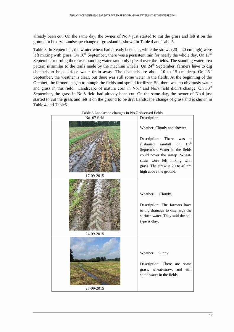
Table 3. In September, the winter wheat had already been cut, while the straws (20 – 40 cm high) were

left mixing with grass. On 16th September, there was a persistent rain for nearly the whole day. On 17

th

September morning there was ponding water randomly spread over the fields. The standing water area

pattern is similar to the trails made by the machine wheels. On 24th September, farmers have to dig

channels to help surface water drain away. The channels are about 10 to 15 cm deep. On 25th

September, the weather is clear, but there was still some water in the fields. At the beginning of the

October, the farmers began to plough the fields and spread fertilizer. So, there was no obviously water

and grass in this field. Landscape of mature corn in No.7 and No.8 field didn’t change. On 30th

September, the grass in No.3 field had already been cut. On the same day, the owner of No.4 just

started to cut the grass and left it on the ground to be dry. Landscape change of grassland is shown in

Table 4 and Table5.

Table 3 Landscape changes in No.7 observed fields.

No. 07 field Description

17-09-2015

Weather: Cloudy and shower

Description: There was a

sustained rainfall on 16th

September. Water in the fields

could cover the instep. Wheat-

straw were left mixing with

grass. The straw is 20 to 40 cm

high above the ground.

24-09-2015

Weather: Cloudy.

Description: The farmers have

to dig drainage to discharge the

surface water. They said the soil

type is clay.

25-09-2015

Weather: Sunny

Description: There are some

grass, wheat-straw, and still

some water in the fields.


16

30-09-2015

Weather: Clear, Sunny

Description: farmers begin to

plough the field with the

fertilizer. There is few grass left

in the fields.

02-10-2015


Description: No water and even

the grass in the fields. The

farmer using the machine to

plough the fields.



25-09-2015

Weather: Sunny

Description: The grass in this

area is about 50 cm to 6o cm

high and wet. When walk across

the grass, it will wet you

clothes. Moreover, the grass is

density and look smooths on the

top

30-09-2015


Description: the owner began to

cut the grass and spread them on

the ground to be dry.


17

02-10-2015


Description: The grass was gone

and ground is getting dry.



25-09-2015

Weather: Sunny

Description: The grass in this

area is about 50 cm to 6o cm

high and wet similar as No.4

field. But a litter bit dry than

No.4 grassland. Moreover, the

grass is also density and look

smooths on the top

30-09-2015


Description: The grass has been

harvested and gathered. The

stems left in the field are 10 cm

to 15 cm high.

02-10-2015


Description: The dry grass was

packed as the white boxes. The

grass left in the ground was

about 10 cm to 15 cm high.


18

5. SENTINEL-1 DATA PRE-PROCESSING

SNAP software (Sentinels Application Platform, http://step.esa.int/main/download/), particularly the

S-1 Tool box of the SNAP was utilized to pre-process the SAR imagery. SAR data can be accessed by

targeting the entire Sentinel ZIP file in SNAP. The original SAR image is inverted in the SNAP. It is

displayed according to the order of data acquisition, which is not according to a cartographic

representation. To reproject the images from geometry of the sensor to the geographic projection,

terrain correction was applied. The influence of the incident angle on the received signal is significant

(G. J.-P. Schumann & Moller, 2015). Particularly in the modes of sensor operation that use the full

swath of the orbit track (O’Grady et al., 2013). Therefore, an incidence angle correction is needed.

Furthermore, the synthetic method used for creating the SAR imagery also has some disadvantages.

Inherent to the measurement technique is random constructive and destructive interference of waves

will cause the SAR images to be noisy. This noise within the SAR images is called speckle and

decreases the quality of the image and making interpretation of features more difficult. A number of

speckle filter types are provided in SNAP. Speckle noise reduction was applied by using single

product speckle filter. Different filter types were simply test by visually comparing the filter results.

Therefore, the data processing including terrain correction, subset, speckle filter, shift by the ground

control points, incidence view angle correction, and convert from intensity (m2 m

-2) to decibel (dB).

The flowchart for data pre-processing is shown below.

Figure 9 Sentinel-1data processing steps

5.1. Terrain correction

Upon completion of the terrain processing a file is created with 3 bands called ‘sigma0_HH’,

‘sigma0_VH’ and ‘ProjectedincidenceAngle’. The ‘ sigma0_VV’ and ‘ sigma0_VH’ bands

include the backscattered cross section in intensity units (m2m

-2). The exploration of the

‘ProjectedIncidenceAngle’ band shows that the incidence angle is expressed in degree.

After Range Doppler Terrain Correction, using bilinear interpolation and SRTM 3sec as Digital

Elevation Model (DEM), there was a shift in longitude of about 9 pixels for the different image passes

(ascending / descending). Other available DEMs in the SNAP tool-box were tested, such as SRTM

1sec, ACE30, but the shift remains. Therefore, ground control points (GCP) were used to georeference

the shifted data. First of all, data were grouped by its ascending and descending passes properties,

which can be found in the Metadata. The cross points of the road in SAR images were selected as

GCPs and then the images are shifted by IDL.

Sentinel-1 images Terrain correction Subset

View angle correction

Convert to dB

Group

SAR data for changing detection Speckle filter

Shift

http://step.esa.int/main/download/


19

5.2. View angle review

Sentinel 1 satellite data are collected at view angle ranging from 29.1° to 46.0°. Incidence angle

describes the angular deviation of the incident signal from nadir. Correction for 𝜎0 differences due to

this angular variability is needed. This is often done by normalizing the observations towards a

reference angle. Besides, the backscatter is dependent on the incidence angle, so to limit the effect of

the incidence angle the backscatter normalization is needed. The most commonly adopted method is

the cosine correction (Mladenova et al., 2012) whereby the 𝜎0 is normalized towards a reference angle

using,

𝜎𝑟𝑒𝑓0 = 𝜎0 𝑐𝑜𝑠𝑛(𝜃𝑟𝑒𝑓 )

𝑐𝑜𝑠𝑛(𝜃𝑣) Equation 1

Where 𝜃𝑣 is the incidence view angle (degrees), 𝜎𝑟𝑒𝑓0 is the normalized backscatter based on a

reference angle, 𝜃𝑟𝑒𝑓 (m2m

−2), and n depends on the type of scattering and ultimately the land cover

characteristics (–) (Velde et al., 2014). In some soil moisture retrieval methods (i.e. Change Detection

techniques) the reference view is often defined as 30 degrees (Dostálová et al., 2014). When

reradiation of the incident energy follows the cosine law, instead of being isotropic, n should be taken

equal to 1, which is in essence an application of Lambert’s law for optics (Velde et al., 2014). This

process was implemented in IDL.

5.3. Speckle filter

Speckle filtering is needed to suppress the noise in order to allow better interpretation and backscatter

analysis. However, speckle filters not only suppress the noise, but also remove observations that are

not affected by noise and contain valuable land surface information (e.g. soil moisture, biomass and

flood extent). Here, single product speckle filter method in SNAP was used to remove the speckle. The

SNAP S1 Tool box operator supports the following speckle filter types for handling speckle noise of

different distributions (Gaussian, multiplicative or Gamma): Mean, Median, Lee, Refined Lee, and

Gamma-MA. Because of the fact that standing water in the observation fields is only 10 m × 5 m

while the pixel size of Sentinel-1 image is 10 m. The window size was defined as 3×3. Figure 10

displays the test result of different filters with same size of moving filter windows on Sentinel-1 image

acquired in 16th September, 2015. Those images illustrate standing water in the No.7 winter wheat

field. According to Figure 10, the Refined Lee filter shows more clear standing water boundary as

highlight in the orange cycle. Because of the standing water area is relatively small compared to the

pixel size of the SAR observations resolution. Refined Lee filter was applied because it maintains the

detail of the standing boundary.

Refine Lee Lee Gamma Map


20

Mean Median Original

Figure 10 Filter results of VH-polarized SAR images acquired on 16-09-2015

An RGB colour composite for visually interpretation (Red and Bule – VV polarization; Green – VH

polarization) was made (Figure 11) for visual interpretation of landscape changes. Combining with

fieldwork observation, it can be observed that the light greenish colour (Figure 11 15-10-2014 ①)

represents the differences between VV and VH backscatter signal, which indicated the presence of

density vegetation, such as forest. The dark greenish colour (Figure 11 16-11-2014 ④) refers to the

grassland, related to its smooth surface. The light purplish colour (Figure 11 16-11-2014 ③) refers to

built-up areas, such as houses. The black areas (Figure 11 15-10-2014 ②)stands for low VV and VH

backscatter signals, related to smooth surface, usually open water bodies and bare soil (Twente

Airport). However, it was also observed that corn fields and winter wheat fields (Figure 11 15-10-2014

⑤) are looks similar, which in purplish. From the visual interpretation for vegetated areas of these

SAR processed images, backscatter of forest is relatively constant during the study period from

October 2014 to September 2015. The backscatter variation in forest is more stable over the year than

the grassland and agricultural fields (corn, winter wheat, grassland). For grassland, the RGB composite

colour doesn’t change frequently throughout the period. This indicates that grass is more constant

However, the RGB colour of winter wheat and corn field as show in Figure 11 ⑤ changes quite often

which is probably due to it vegetation growth, surface conditions changes.

15-10-2014 16-11-2014 14-12-2014

1 2

3

4

5


21

15-01-2015 15-02-2015 16-03-2015

16-04-2015 15-05-2015 17-06-2015

14-07-2015 14-08-2015 16-09-2015

Figure 11 Backscatter (in dB) for RGB colour composite (Green--VH polarization; Red and Blue--VV

polarization) at different dates.


22

6. BACKSCATTER ANALYSIS

6.1. Image based backscatter analysis

Based on the previous study, estimators for backscatter temporal variability were tested in this area.

The other calculated results are displayed in Figure 12 with RGB colour composite (Green--VH

polarization; Red and Blue--VV polarization) for visual interpretation. According to the Figure 12(a,b),

saturation map and Maximum minus minimum ratio map do not provide a clear characteristics of

backscatter for land cover classification. Combining with the land cover map shown in Figure 5, it can

be seen that the purplish colour shown in the Figure 12(c) refers to the urban area and the white color

in Figure 12 (d) indicates the smooth surface targets, like airport and open water body.

(a) Saturation (b) Maximum-Minimum ratio in dB

(c) Logarithmic measure based on normalized Standard deviation

(d) Normalized standard devition

Figure 12 Backscatter temporal variability calculated by different estimators for RGB colour composite (Green--

VH polarization; Red and Blue--VV polarization) at different dates : (a) Saturation backscatter; (b) Maximum-

Minimum Ratio in dB; (c) Logarithmic measure based on normalized Standard deviation; (d) Normalized

standard devition

Compared to the above 4 estimators, standard deviation of dB values and mean backscatter show the

relatively better distinguish for most land cover classification. Therefore, in this research, standard

deviation of dB Values (Equation 2) and mean VV and VH polarized backscatter were calculated to

analyse the temporal backscatter variability.


23

Standard Deviation of dB Values:

stdev = √1

N∗ ∑ (10 ∗ log10σi)

2 − (1

N∗ ∑ 10 ∗N

i=1 log10σi)2

Ni=1 Equation 2

where 𝜎𝑖 is the backscatter coefficient of image i. There are N images in total.

(a) Mean backscatter (in dB)

(b) Standard deviation of backscatter (in dB)

Figure 13 Backscatter statistics result for RGB colour composite (Green--VH polarization; Red and Blue--VV

polarization): (a) mean backscatter (in dB); (b) standard deviation of backscatter (in dB)

1 2

3

5

4

5

1 2 3

4


24

Figure 13 shows an RGB colour composite (Red and Bule – VV polarization; Green – VH polarization)

was made from average backscatter statistic image and standard deviation (stdev) map of VH and VV-

polarized backscatter for visual interpretation. Combining with fieldwork observation, it can be

observed from the mean backscatter map (Figure 13 a) that the greenish color (Figure 13 a ①)

indicates the presence of forest. While in the stdev map (Figure 13 b) forest is in a dark tone because

they are much more stable not changed much by the rainfall and its growth stage. The bright purplish

colour in the Figure 13(a ②) refers to the urban areas. Although urban is the most stable land cover

compared to others, urban shows a light colour in stdev map due to surface building material, trees

canopy effect, and noisy. The black areas in Figure 13 (a ③) stands for low VV and VH backscatter

signals which belongs to open water bodies, roads and bare soil (Twente Airport). However, open

water body is not very outstanding in the stdev map. For agricultural fields, the dark greenish color in

Figure 13(a ④) represent the grassland, related to densely leaves and smooth surface. However, the

corn fields and winter wheat fields have a similar colour (purplishFigure 13 a ⑤ ) in average

backscatter image. While in stdev map, corp field are more markble which in the greenish colour.

Possible resaon for the different colour in those two map may be due to the landscape seasonal change

from roughness bare soil to the densely crop covers.

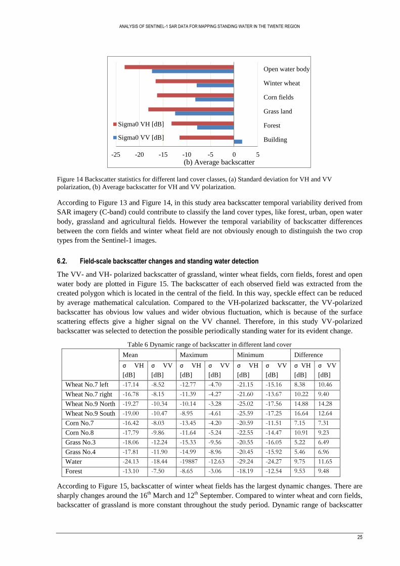
Based on the backscatter statistic results, temporal variation of backscatter and mean backscatter for

different land cover were extracted by zonal statistics in ENVI software. According to the Figure 14,

open water body has the lowest backscatter due to the specular reflection over the smooth water

surface, and simlar standard deviation as grassland. This is possibly due to waves on the water surface

caused by the wind and the aquatic plant. Temporal variability of forest is the lowest while forest has

higher average backscatter because its typically contant over time and less affected by the surface

conditions. Relatively higher standard deviation is found in agricultural field, including corn fields and

winter wheat. Because of the seasonality of agricultural activity, soil moisture changes and weather

conditions, corn fields and winter wheat fields have higher standard deviation compared to the

grassland.

0 1 2 3 4 5

Building

Forest

Grass land

Corn fields

Winter wheat

Open water body

(a) Standard deviation

Sigma0 VH [dB]

Sigma0 VV [dB]


25

Figure 14 Backscatter statistics for different land cover classes, (a) Standard deviation for VH and VV

polarization, (b) Average backscatter for VH and VV polarization.

According to Figure 13 and Figure 14, in this study area backscatter temporal variability derived from

SAR imagery (C-band) could contribute to classify the land cover types, like forest, urban, open water

body, grassland and agricultural fields. However the temporal variability of backscatter differences

between the corn fields and winter wheat field are not obviously enough to distinguish the two crop

types from the Sentinel-1 images.

6.2. Field-scale backscatter changes and standing water detection

The VV- and VH- polarized backscatter of grassland, winter wheat fields, corn fields, forest and open

water body are plotted in Figure 15. The backscatter of each observed field was extracted from the

created polygon which is located in the central of the field. In this way, speckle effect can be reduced

by average mathematical calculation. Compared to the VH-polarized backscatter, the VV-polarized

backscatter has obvious low values and wider obvious fluctuation, which is because of the surface

scattering effects give a higher signal on the VV channel. Therefore, in this study VV-polarized

backscatter was selected to detection the possible periodically standing water for its evident change.

Table 6 Dynamic range of backscatter in different land cover

Mean Maximum Minimum Difference

σ VH

[dB]

σ VV

[dB]

σ VH

[dB]

σ VV

[dB]

σ VH

[dB]

σ VV

[dB]

σ VH

[dB]

σ VV

[dB]

Wheat No.7 left -17.14 -8.52 -12.77 -4.70 -21.15 -15.16 8.38 10.46

Wheat No.7 right -16.78 -8.15 -11.39 -4.27 -21.60 -13.67 10.22 9.40

Wheat No.9 North -19.27 -10.34 -10.14 -3.28 -25.02 -17.56 14.88 14.28

Wheat No.9 South -19.00 -10.47 -8.95 -4.61 -25.59 -17.25 16.64 12.64

Corn No.7 -16.42 -8.03 -13.45 -4.20 -20.59 -11.51 7.15 7.31

Corn No.8 -17.79 -9.86 -11.64 -5.24 -22.55 -14.47 10.91 9.23

Grass No.3 -18.06 -12.24 -15.33 -9.56 -20.55 -16.05 5.22 6.49

Grass No.4 -17.81 -11.90 -14.99 -8.96 -20.45 -15.92 5.46 6.96

Water -24.13 -18.44 -19887 -12.63 -29.24 -24.27 9.75 11.65

Forest -13.10 -7.50 -8.65 -3.06 -18.19 -12.54 9.53 9.48

According to Figure 15, backscatter of winter wheat fields has the largest dynamic changes. There are

sharply changes around the 16th March and 12

th September. Compared to winter wheat and corn fields,

backscatter of grassland is more constant throughout the study period. Dynamic range of backscatter

-25 -20 -15 -10 -5 0 5

Building

Forest

Grass land

Corn fields

Winter wheat

Open water body

(b) Average backscatter

Sigma0 VH [dB]

Sigma0 VV [dB]


26

change of different land cover is shown in Table 6. Grassland has the minor fluctuation and the

dynamic range is 6.49 dB and 6.96 dB for VV- polarization in each observed field No.3 and No.4.

High fluctuation is found in No.9 winter wheat field varying from -17.56 dB to -3.28 dB. While the

fluctuation range in No.7 winter wheat fields is between -15.16 dB to -4.70 dB for left land and -13.67

dB to -4.26 dB for right part. The range difference of backscatter of corn field No.7 and No.8 is 7.31

dB and 9.23 dB, respectively. It also can be seen from the Figure 15 that backscatter changes varies

from different land cover types and different location fields with the effect of surface conditions,

atmospheric forcings and vegetation characteristics.

Winter wheat field (VV-polarized backscatter) Winter wheat field (VH-polarized backscatter)

Corn field (VV-polarized backscatter) Corn field (VH-polarized backscatter)

Grassland (VV-polarized backscatter) Grassland (VH-polarized backscatter)

Figure 15 Backscatter changes of different land cover

As described in the section 6.1, open water has the lowest backscatter due to its smooth surface. Forest

has higher average backscatter because its typically contant over time and less affected by the surface

conditions. Here, backscatter changes of forest and open water body are plotted as the thresholding for


27

detecting the possible periodically standing water. It is expected that the low backscatter in each

agricultural field which is close to the open water body backscatter may be probably because of the

standing water. However, changes in land surface conditions (e.g. soil moisture, vegetation biomass)

due to atmospheric forcings, and human activities, like ploughing, seeding, and harvesting, affect the

backscatter signal observed by Sentinel-1. In the next section, possible periodically standing water was

verified with considering effect of the in-situ rainfall, soil moisture, and vegetation biomass.

6.3. Temporal verification

In this section, possible periodically standing water was verified using different ancillary data sets

such as the in-situ rainfall, soil moisture, and vegetation biomass (NDVI). In-situ rainfall pattern, soil

moisture pattern of the whole study area and vegetation biomass of each observed field are first

described in 6.3.1 and 6.3.2. Among all the observed fields, No.7 winter wheat field had the obvious

surfacing water in the field mixing the wheat-straw and grass in September. While wider fluctuation

was found in No.9 winter wheat field. The soil moisture station is built in the right side of No.7 wheat

field and north part of No.9 filed. However, some soil moisture measurement data of No.7 station is

missing. In order to better verify the possible standing water area here we chose No.9 north part winter

wheat field and No.4 grassland as test examples to verify the periodically standing water. The

verification of possible periodically standing water will be discussed in section 6.3.3 and

6.3.4considering with ancillary data.

6.3.1. Rainfall and soil moisture trend

Figure 16 shows the daily rainfall of Twente station from October 2014 to September 2015. According

to Figure 16, rainfall nearly spread out the study period with several rainfall peaks and very intensive

rain events. There are two rainfall peaks in July and August, where the daily rainfall is more than 25

mm. The accumulation precipitation is 821.8 mm. As the observed fields are far away from river, the

main source of water is from rainfall. Therefore, standing water is generated either by rainfall failing

to infiltration because of low infiltration capacity or by precipitation falling on to already saturation

ground. It also can be seen that soil moisture averaged from all 20 stations is in a good agreement with

the rainfall pattern. From December to June, there is an obvious increasing trend of soil moisture with

increasing rainfall or intensive rainfall events. However, the fluctuation of soil moisture is not very

significantly in the July and August as there was two rainfall peaks.

Figure 16 Daily rainfall data collected from Twente station, and the soil moisture data averaged from the 20 soil

moisture network stations in Tewnte from October 2014 to September 2015.

0

5

10

15

20

25

30

35

40

0.000

0.050

0.100

0.150

0.200

0.250

0.300

0.350

0.400

0.450

0.500Soil Moisture

Rainfall

So

il m

ois

ture

[m

3/m

3] R

ainfall [m

m]

Date


28

6.3.2. NDVI for agricultural fields

Figure 17 shows the NDVI for all observed field which were used to describe the relative density and

biomass of vegetation. Furthermore, it is also used as an indicator for the agricultural activities (e.g.,

harvest). It can be seen from Figure 17, the same land cover type shows almost similar increasing and

decreasing trends throughout the study period. According to Figure 17 (a,b), around the 20th April

there is a markedly increasing of NDVI. Possible reason for the strong change may be due to the fact

that wheat is start growing. In August, NDVI curves of wheat field decline significantly from the

peaks (0.78) to the low point (0.32) which is related to the harvest. Although it is not very clear shown

in the NDVI curve, it can be concluded that ploughing, seeding, would be done during October to

January because the NDVI is kept low and changes slightly during the period. From October to

January, the variation of NDVI in field No.7 is about 0.04, and there is almost no change in No.9 field.

For corn field (Figure 17 c,d), the corn is growing faster from June and getting mature in October as

the NDVI value changes from 0.31 to 0.75 and remain stable. In October, 2014, NDVI for No.7 corn

field declines from 0.62 to 0.21. However, NDVI curve of No.8 field is much stable around 0.28. This

is probably indicates that within study area corn was harvest at different time in 2014. Corn in No.7

field was harvest in October and corn in No.8 field had already been harvest before the October.

Compared to the winter wheat and corn fields, NDVI of grassland is much higher. The average NDVI

is 0.62 throughout the study period. Besides, NDVI curves of grassland increasing and decreasing

more frequently which is probably due to the harvest as shown in Figure 17 (e,f).

(a) No.7 Winter wheat field (b) No.9 Winter wheat field

(c) No.7 Corn field (d) No.8 Corn field

00.10.20.30.40.50.60.70.80.9

No7_wheat left No.7_wheat right

ND

VI

Date

00.10.20.30.40.50.60.70.80.9

No9_wheat_North No9_wheat_South

ND

VI

Date

00.10.20.30.40.50.60.70.80.9

No7_corn

ND

VI

Date

00.10.20.30.40.50.60.70.80.9

No8_corn

ND

VI

Date


29

(e)No.3 Grassland (f) No.4 Grassland

Figure 17 NDVI for corn fields, winter wheat field and grassland.

6.3.3. Periodically standing water in winter wheat field

According to Figure 15, fluctuation of backscatter from two non-adjacent winter wheat fields is quite

different. The variation of backscatter in No.9 field is larger than No.7 field. The backscatter is also

smaller than No.7 field. Particularly, it is clearly seen that the backscatter of No.9 field in September is

much lower than the No.7. During the fieldwork period, No.7 and No.9 field had been visited on 24th

September. Based on the observation, there was no standing water in the No.9 although the backscatter

derived from No.9 north part field is much lower than No.7 field. In No.7 right part wheat field,

standing water spread randomly mixing with the wheat-straw and grass as shown in Figure 8. While in

No.9 field, the surface was smooth with sparse grass. Possible reason for the higher backscatter in

No.7 field may be due to the wet soil moisture. The increase of the soil dielectric constant with water

content leads to an enhanced signal return. In addition, rough surface also increases the backscatter

signal observed by Sentinel-1.

(a) Rainfall with backscatter [dB] backscatter of No.9 wheat field

00.10.20.30.40.50.60.70.80.9

No3_grassDate

ND

VI

00.10.20.30.40.50.60.70.80.9

No4_grass

Date

ND

VI

0

5

10

15

20

25

30

35

40-30

-25

-20

-15

-10

-5

0

5

10

20

14

10

01

20

14

10

18

20

14

11

04

20

14

11

21

20

14

12

08

20

14

12

25

20

15

01

11

20

15

01

28

20

15

02

14

20

15

03

03

20

15

03

20

20

15

04

06

20

15

04

23

20

15

05

10

20

15

05

27

20

15

06

13

20

15

06

30

20

15

07

17

20

15

08

03

20

15

08

20

20

15

09

06

20

15

09

23

No9_wheat_σVV Rainfall

V

V-p

ola

rize

d B

acksc

atte

r [d

B] R

ainfall [m

m]

Date


30

(b) Soil moisture with backscatter [dB] of No.9 wheat field

Figure 18 Soil moisture with backscatter of No.9 field and daily rainfall derived from Twente station.

Figure 18 shows the soil moisture with backscatter of No.9 field and daily rainfall derived from

Twente station. In general, soil moisture is in a good agreement with the rainfall. When there is a

rainfall event or consist rainfall event, the soil moisture is increasing. According to Figure 18,

backscatter around 12th June is relatively lower about -15.04 dB, however, the NDVI in June has

reached the peak (0.72). Around 12th June, there is less rainfall, more importantly, the soil moisture

during this period is lower than 0.2 m3m

-3. Therefore, the low backscatter happens around 12

th June is

probably due to the low soil moisture instead of the standing water. Compared to vegetation biomass,

soil moisture is the dominant factors in backscatter. In addition, in 23rd

March, there is a sharply

changes of backscatter and the backscatter decreases from -6.41 dB to -15.44 dB. Because the

consistent rainfall events, the soil moisture in March is higher than 0.3 m3m

-3. As the NDVI in March

is much lower, the low backscatter in March probably due to the periodically standing water. On the

other hand, the NDVI curve shows that the vegetation in No.9 winter wheat field is slightly increasing

from the 24th March. The farmer activities like seeding could also affect the backscatter. Besides, there

is decreasing trend of backscatter declines from -5.78 dB in 28th March to -15.43dB in 18

th April. This

is probably because the decreasing trend of rainfall during the same time.

6.3.4. Periodically standing water in grassland

Figure 19 shows the soil moisture with backscatter of No.4 field and daily rainfall derived from

Twente station. As shown in Table 6, the backscatter of grassland is much lower compared to the

winter wheat and corn fields. However, NDVI of grassland is consistent and relatively higher

throughout the study period as shown in Figure 17. The average NDVI of No.3 and No.4 field is 0.81

and 0.77, respectively. According to Figure 19, the backscatter trend is in a good agreement with the

soil moisture curve before May, and the soil is extremely wet as the soil moisture is close to 0.6. It can

be observed that the increasing trend of backscatter with increasing soil moisture in a densely biomass

situations from January to May, 2015. However, during the same period, the backscatter is quite lower

than other crop types. The possible reason for this may be due to the standing water, and it seems that

vegetation biomass has less influent on backscatter changes.

0.000

0.100

0.200

0.300

0.400

0.500

0.600

-30

-25

-20

-15

-10

-5

0

5

10No9_wheat_σVV

Soil moisture_No.9V

V-p

ola

rize

d B

acksc

atte

r [d

B]

So

il mo

istire [m3/m

3]

Date


31

(a) Rainfall with backscatter [dB] backscatter of No.9 wheat field

(b) Soil moisture with backscatter [dB] of No.4 grassland

Figure 19 Soil moisture with backscatter [dB] of No.4 field and daily rainfall derived from Twente station

05101520253035404550-30

-25

-20

-15

-10

-5

0

5

10

20

14

10

01

20

14

10

20

20

14

11

08

20

14

11

27

20

14

12

16

20

15

01

04

20

15

01

23

20

15

02

11

20

15

03

02

20

15

03

21

20

15

04

09

20

15

04

28

20

15

05

17

20

15

06

05

20

15

06

24

20

15

07

13

20

15

08

01

20

15

08

20

20

15

09

08

20

15

09

27

VV-polarized σ Rainfall

VV

-po

lari

zed

Bac

ksc

atte

r [d

B]

Rain

fall [mm

]

Date

0.000

0.100

0.200

0.300

0.400

0.500

0.600

-30

-25

-20

-15

-10

-5

0

10/1/14…

11/1/14…

12/1/14…

1/1/15…

2/1/15…

3/1/15…

4/1/15…

5/1/15…

6/1/15…

7/1/15…

8/1/15…

9/1/15…

No4_grass_σVV Soil moisture _No4

V

V-p

ola

rize

d B

acksc

atte

r [d

B]

Soil m

oistire [m

3/m3]

Date


32

7. CONCLUSION AND RECOMMENDATION

7.1. Conclusions

The main objective for this study aims to analyse Sentinel-1 data for its potential to map standing

water in agricultural fields. A series of Sentinel-1 SAR images were used to detect the possible

periodically standing water based on backscatter temporal variability and backscatter changes on field

scale. Ancillary data, like soil moisture, rainfall, and NDVI were applied to verify the possible

periodically standing water area. In addition, fieldwork has been done from 17th September 2015 to

2nd

October 2015 in order to find the standing water in different kinds of agricultural fields. There are

6 fields had been visited including two grassland, two corn fields and two winter wheat fields. Only

one winter wheat field (No.7 field) had obvious surface water. Standing water in one grassland (No.4

field) spread as mosaic under the thick grass. Moreover, the time of landscape changes and agricultural

activities were recorded in order to analyse backscatter changes with respect to land surface conditions.

The following conclusions are drawn from the analyses results.

· Standard deviation in dB and mean backscatter were calculated to show the backscatter temporal

variation for a series SAR images. Open water body has the lowest backscatter (-18.44 dB VV-

polarized backscatter) due to the specular reflection over the smooth water surface. It has the

simlar standard deviation with grassland. The standard deviation of open water body and grassland

are 2.03 and 2.12, respectively. This is possibly due to waves on the water surface caused by the

wind and the aquatic plant. Urban has the highest backscatter (-3.46 dB VV-polarized backscatter)

and highest standard devation (2.8) which probably with respect to the material of the buiding,

cars on the road. Because of the volume scatter caused by the canopy and branches, forest has

higher average backscatter (-7.49 dB VV-polarized backscatter). Temporal variability of forest

(1.97) is the lowest because its typically contant over time and less affected by the surface

conditions. Relatively higher standard deviation is found in agricultural fields, including corn

fields (2.60) and winter wheat (2.57). Because of the seasonality of agricultural activity, soil

moisture changes and weather conditions, corn fields and winter wheat have higher standard

deviation compared to the grassland (2.12). In addition, the mean VV-polarized backscatter of

winter wheat field is -8.25 dB which is similar to the corn field (-7.96 dB). These results show that

multi-temporal backscatter observations can be used to classify the agricultural field from forest,

urban, open water body and grassland. However, because of the effect of surface roughness, soil

moisture and vegetation growth, winter wheat and corn field are difficult to distinguish.

· Changes in land surface conditions (e.g. soil moisture, vegetation biomass) due to atmospheric

forcings, and human activities, like ploughing, seeding, and harvesting, affect the backscatter

signal observed by Sentinel-1. Among all the possible influence factors, soil moisture is the

dominant factors in backscatter change. The vegetation biomass in winter wheat fields and

grassland is not a significant factor contributing to the backscatter changes.

· Based on the field-scale backscatter changes, standing water is difficult to delineate from the

Sentnel-1 images due to the uncertainties. Those uncertainties include different surface conditions

in each agricultural field, soil moisture, vegetation characteristics and agricultural activities. Those

factors vary from temporal and spatial scale, like farming practices and atmospheric forcings.

7.2. Limitations and recommendations

· Due the ascending and descending of the sensor and the bug in the SNAP S1 tool box, there was a

shift of the SAR images after the terrain correction. Then GCPs like roads cross points were used


33

to shift the images in order to overlay all the layers. However, by shift the image based on GCPs

the accuracy has been a little bit decreased.

· The standing water area in observation is as much as 10 m × 5 m randomly distributed in the

fields. However, the resolution of Sentinel-1 images is 10 m. One problem would be that the

standing water area is relatively small compared to the pixel size of the SAR observations.

· Limited number of standing water area has been found during the fieldwork period. Among 6

observed fields, only one winter wheat field has obvious standing water, and one grassland field

has standing water underneath the densely grass. The number of observed standing water fields for

analysis Sentinel-1 potential for mapping standing water is not enough. Therefore, the observation

time should last longer in order to find enough observation standing water samples.

· In addition, in this study polygons were made for each observed field, which was used to extract

the backscatter coefficient. Those regions of interesting were created in the center of the field in

order to avoid the interference of the field boundary effect, such as tree canopy. Also, the

backscatter of each observed field will be approximated by averaging calculation in order to

decrease the effects of speckle. However, backscatter derived from a region will cause the signal

of standing water mixed with other surface signals, which will add uncertainty to the result.

· Attention should be paid to the timing of the standing water and the interval time of the SAR

images (e.g. when there will be standing water and its duration). The interval time of SAR images

in this study very from 2 to 11 days.

· Among the study area, agricultural activities like the ploughing, seeding, harvest start at different

time which depends on the crop type and farmer’s time schedule. Therefore，we have limited

information about the field conditions, for example, surface roughness, grass cover, what had been

left after the harvest. Because those factors would affect the signal of observation. In order to

better understand the backscatter changes, more information about the crop and landscape in the

field should be collected.

· Larger area of standing water should be found to reduce the effect of grass, roughness soil around

the water.

· More quantitative measurements of the standing water area should be collected for the further

validation

35

LIST OF REFERENCES

ASAR - Earth Online - ESA. (n.d.). Retrieved August 26, 2015, from https://earth.esa.int/web/guest/missions/esa-operational-eo-missions/envisat/instruments/asar

Attema, E., Davidson, M., Snoeij, P., Rommen, B., Floury, N., & Agency, E. S. (2009). SENTINEL-1 MISSION OVERVIEW, 36–39.

Bazi, Y., Bruzzone, L., & Melgani, F. (2007). Image thresholding based on the EM algorithm and the generalized Gaussian distribution. Pattern Recognition, 40(2), 619–634. http://doi.org/10.1016/j.patcog.2006.05.006

Berning, C., Viljoen, M. F., & Du Plessis, L. A. (2000). Loss functions for sugar-cane: Depth and duration of inundation as determinants of extent of flood damage. Water SA, 26(4), 527–530.

Bruzzone, L., Marconcini, M., Wegmüller, U., & Wiesmann, A. (2004). An advanced system for the automatic classification of multitemporal SAR images. IEEE Transactions on Geoscience and Remote Sensing, 42(6), 1321–1334. http://doi.org/10.1109/TGRS.2004.826821

Cloude, S. (2009). Polarisation: Applications in Remote Sensing. Retrieved from https://books.google.com/books?hl=zh-CN&lr=&id=c67UPCcbfHUC&pgis=1

Dente, L., Su, Z., & Wen, J. (2012). Validation of SMOS soil moisture products over the Maqu and Twente Regions. Sensors, 12(8), 9965–9986. http://doi.org/10.3390/s120809965

Dente, L., Vekerdy, Z., Su, Z., & Ucer, M. (2011). Soil Moisture and Soil Temperature Monitoring Network.

Di Baldassarre, G., Schumann, G., & Bates, P. D. (2009). A technique for the calibration of hydraulic models using uncertain satellite observations of flood extent. Journal of Hydrology, 367(3-4), 276–282. http://doi.org/10.1016/j.jhydrol.2009.01.020

Dostálová, A., Doubková, M., Sabel, D., Bauer-Marschallinger, B., & Wagner, W. (2014). Seven Years of Advanced Synthetic Aperture Radar (ASAR) Global Monitoring (GM) of Surface Soil Moisture over Africa. Remote Sensing, 6, 7683–7707. http://doi.org/10.3390/rs6087683

ERS overview / Observing the Earth / Our Activities / ESA. (n.d.). Retrieved August 26, 2015, from http://www.esa.int/Our_Activities/Observing_the_Earth/ERS_overview

Giustarini, L., Hostache, R., Matgen, P., Schumann, G. J., Bates, P. D., & Mason, D. C. (2013). A Change Detection Approach to Flood Mapping in Urban Areas Using TerraSAR-X. IEEE Transactions on Geoscience and Remote Sensing, 51(4), 2417–2430. http://doi.org/10.1109/TGRS.2012.2210901

Gstaiger, V., Huth, J., Gebhardt, S., Wehrmann, T., & Kuenzer, C. (2012). Multi-sensoral and automated derivation of inundated areas using TerraSAR-X and ENVISAT ASAR data. International Journal of Remote Sensing, 33(22), 7291–7304. http://doi.org/10.1080/01431161.2012.700421

Henry, J. ‐B., Chastanet, P., Fellah, K., & Desnos, Y. ‐L. (2006). Envisat multi‐polarized ASAR data

for flood mapping. International Journal of Remote Sensing, 27(10), 1921–1929. http://doi.org/10.1080/01431160500486724

Hostache, R., Matgen, P., & Wagner, W. (2012). Change detection approaches for flood extent mapping: How to select the most adequate reference image from online archives? International Journal of Applied Earth Observation and Geoinformation, 19(1), 205–213. http://doi.org/10.1016/j.jag.2012.05.003

36

Kuenzer, C., Guo, H., Huth, J., Leinenkugel, P., Li, X., & Dech, S. (2013). Flood mapping and flood dynamics of the mekong delta: ENVISAT-ASAR-WSM based time series analyses. Remote Sensing, 5(2), 687–715. http://doi.org/10.3390/rs5020687

Matgen, P., Hostache, R., Schumann, G., Pfister, L., Hoffmann, L., & Savenije, H. H. G. (2011). Towards an automated SAR-based flood monitoring system: Lessons learned from two case studies. Physics and Chemistry of the Earth, 36(7-8), 241–252. http://doi.org/10.1016/j.pce.2010.12.009

Mladenova, I. E., Jackson, T. J., Bindlish, R., & Hensley, S. (2012). Incidence Angle Normalization of Radar Backscatter Data. Geoscience and Remote Sensing, IEEE Transactions on, 51(3), 1791–1804. http://doi.org/10.1109/TGRS.2012.2205264

Mtamba, J., van der Velde, R., Ndomba, P., Zoltán, V., & Mtalo, F. (2015). Use of Radarsat-2 and Landsat TM Images for Spatial Parameterization of Manning’s Roughness Coefficient in Hydraulic Modeling. Remote Sensing, 7(1), 836–864. http://doi.org/10.3390/rs70100836

O’Grady, D., Leblanc, M., & Gillieson, D. (2013). Relationship of local incidence angle with satellite radar backscatter for different surface conditions. International Journal of Applied Earth Observation and Geoinformation, 24, 42–53. http://doi.org/10.1016/j.jag.2013.02.005

Pulvirenti, L., Chini, M., Pierdicca, N., Guerriero, L., & Ferrazzoli, P. (2011). Flood monitoring using multi-temporal COSMO-SkyMed data: Image segmentation and signature interpretation. Remote Sensing of Environment, 115(4), 990–1002. http://doi.org/10.1016/j.rse.2010.12.002

Pulvirenti, L., Pierdicca, N., Chini, M., & Guerriero, L. (2011). An algorithm for operational flood mapping from Synthetic Aperture Radar (SAR) data using fuzzy logic. Natural Hazards and Earth System Science, 11(2), 529–540. http://doi.org/10.5194/nhess-11-529-2011

Schlaffer, S., Matgen, P., Hollaus, M., & Wagner, W. (2015). Flood detection from multi-temporal SAR data using harmonic analysis and change detection. International Journal of Applied Earth Observation and Geoinformation, 38, 15–24. http://doi.org/10.1016/j.jag.2014.12.001

Schumann, G., Di Baldassarre, G., & Bates, P. D. (2009). The utility of spaceborne radar to render flood inundation maps based on multialgorithm ensembles. IEEE Transactions on Geoscience and Remote Sensing, 47(8), 2801–2807. http://doi.org/10.1109/TGRS.2009.2017937

Schumann, G. J.-P., & Moller, D. K. (2015). Microwave remote sensing of flood inundation. Physics and Chemistry of the Earth, Parts A/B/C. http://doi.org/10.1016/j.pce.2015.05.002

Sentinel-1 Team. (2013). Sentinel-1 User handbook. http://doi.org/GMES-S1OP-EOPG-TN-13-0001

Ticehurst, C. J., Dyce, P., & Guerschman, J. P. (2009). Using passive microwave and optical remote sensing to monitor flood inundation in support of hydrologic modelling. 18th World IMACS / MODSIM Congress, Cairns, Australia, (July), 3747–3753. Retrieved from http://mssanz.org.au/modsim09

Torres, R., Snoeij, P., Geudtner, D., Bibby, D., Davidson, M., Attema, E., … Rostan, F. (2012). GMES Sentinel-1 mission. Remote Sensing of Environment, 120, 9–24. http://doi.org/10.1016/j.rse.2011.05.028

Townsend, P. a., & Walsh, S. J. (1998). Modeling floodplain inundation using an integrated GIS with radar and optical remote sensing. Geomorphology, 21(3-4), 295–312. http://doi.org/10.1016/S0169-555X(97)00069-X

37

Velde, R. Van Der, Salama, M. S., Eweys, O. A., Wen, J., & Wang, Q. (2014). Active / Passive Microwave Observations Over the East of the Netherlands, 1–18.

Documents

Analysis of Sentinel-1 SAR data for mapping standing water