Embed Size (px)
Citation preview

i
ANALYSIS OF SOFT COMPUTING
TECHNIQUES FOR FACE DETECTION
Thesis submitted in partial fulfillment of the requirements for the award of degree of
Master of Engineering
in
Software Engineering
By:
Tarun Kumar
(800831015)
Under the supervision of:
Mr. Karun Verma
Assistant Professor
COMPUTER SCIENCE AND ENGINEERING DEPARTMENT
THAPAR UNIVERSITY
PATIALA – 147004
June 2010

i

ii

iii
Dedicated to my beloved
family

iv
Abstract
Soft computing techniques are a good solution for the face detection. Neural network is
one of the soft computing techniques, which are generally used for learning and training
process. Face detection is one of the challenging problems in the image processing. The
basic aim of face detection is determine if there is any face in an image. And then locate
position of a face in image. Human face detected in an image can represent the presence
of a human in a place. Evidently, face detection is the first step towards creating an
automated system, which may involve other face processing. A novel face detection
system is presented in this research work. The approach relies on neural networks, which
can be used to detect faces by using FFT. The neural network is created and trained with
training set of faces and non-faces. The network used is a two layer feed-forward neural
network. There are two modifications for the classical use of neural networks in face
detection. First, the neural network tests only the face candidate regions for faces, thus
the search space is reduced. Second, the window size used by the neural network in
scanning the input image is adaptive and depends on the size of the face candidate region.
The objective of this work was to implement a classifier based on MLP (Multi-layer
Perception) neural networks for face detection. The MLP was used to classify face and
non-face patterns.
Soft computing techniques, which emphasize gains in understanding system behavior in
exchange for unnecessary precision, have proved to be important practical tools for many
existing problems. NNs are approximations of any multivariate function because they can
be used for modeling highly nonlinear, unknown, or partially known complex systems,
plants, or processes. We made four combinations FFT_TRAINSCG, DCT_TRAINSCG,
FFT_TRAINCGB and DCT_TRAINCGB for face detection and compare the results.

v
Table of Contents
Certificate ...................................................................................................................... i
Acknowledgement ..............................................................Error! Bookmark not defined.
Abstract ........................................................................................................................ iv
Table of Contents ...........................................................................................................v
List of Figures ............................................................................................................ viii
List of Table ...................................................................................................................x
Chapter 1 Introduction .................................................................................................1
1.1 Human face Detection in Visual Scenes .................................................................1
1.2 Neural Network ......................................................................................................2
1.2.1 Neurons:.......................................................................................................3
1.3 Basic concepts of Neural Networks ........................................................................4
1.3.1 Network Properties .......................................................................................4
1.3.2 Node Properties ............................................................................................6
1.3.3 System Dynamics .........................................................................................8
1.4 Application area ................................................................................................... 11
1.4.1 Application in image processing ................................................................. 11
1.4.2 Business Applications in industry ............................................................... 11
1.4.3 Application of Feed forward Neural Networks: .......................................... 12
1.5 Advantages of Neural Networks ........................................................................... 13
1.6 Image Processing ................................................................................................. 13
1.6.1 Image types ................................................................................................ 14
1.6.2 Resolution .................................................................................................. 15
1.6.3 Gray levels ................................................................................................. 15
1.6.4 RGB Color model ..................................................................................... 16
1.6.5 Histogram .................................................................................................. 18

vi
1.6.6 Segmentation: ............................................................................................ 18
1.6.7 Image enhancement .................................................................................... 19
1.6.8 Canny Edge Detection ................................................................................ 19
1.6.9 Sobel Edge Detection ................................................................................. 20
Chapter 2 Review of the State of the Art / Literature Review ................................... 21
2.1 Survey on neural network base Face detection ...................................................... 21
2.2. Techniques .......................................................................................................... 26
2.2.1. Knowledge based method .......................................................................... 26
2.2.2 Image Based method: ................................................................................. 27
2.2.3 Features Based method ............................................................................... 27
2.2.4 Template matching method ........................................................................ 27
Chapter 3 Problem Statement and Methodology ....................................................... 29
3.1 Problem Statement ............................................................................................... 29
3.2 Motivation............................................................................................................ 30
3.3 Methodology ........................................................................................................ 31
Chapter 4 Implementation of Face Detection Algorithm ........................................... 32
4.1 What Is MATLAB ............................................................................................... 32
4.2 Neural Network Toolbox.........................................................................................33
4.2.1 Introduction to the GUI .............................................................................. 33
4.2.2 Create a neural Network (nntool):............................................................... 33
4.2.3 Input and Target ......................................................................................... 33
4.2.4. Create Network: ........................................................................................ 35
4.2.5. Train the Neural network ........................................................................... 36
4.3 Performance Functions ......................................................................................... 36
4.3.1 Description of msereg: ............................................................................... 37
4.4 Training Functions ............................................................................................... 37
4.4.1 Description of trainscg ............................................................................... 38

vii
4.4.2 Description of Traincgb .............................................................................. 39
4.5 Layer Initialization Functions ............................................................................... 40
4.5.1 Description of Initlay.................................................................................. 40
4.6 Image Processing Toolbox ................................................................................... 40
4.7 Architecture for face detection.............................................................................. 41
4.8 Histogram equalization ......................................................................................... 42
4.9 Transformation.......................................................................................................42
4.10 Gabor filters ....................................................................................................... 43
4.11 Selection of network architecture........................................................................ 45
4.11.1 How Many Hidden Layers are enough ...................................................... 45
4.11.2. How Many Hidden Neurons are enough .................................................. 46
4.12 Training algorithm and image testing .......................................................... 47
Chapter 5 Result and Testing ...................................................................................... 49
5.1. Result of FFT_TRAINSCG ................................................................................. 49
5.2. Result of DCT_TRAINSCG ................................................................................ 52
5.3. Result of FFT_TRAINCGB ................................................................................ 54
5.4. Result of DCT_TRAINCGB ............................................................................... 57
5.5 Comparison of result ............................................................................................ 59
5.6 Performance Analysis........................................................................................... 60
Chapter 6 Conclusion and Future scope ..................................................................... 61
6.1 Conclusion ........................................................................................................... 61
6.2 Future scope ......................................................................................................... 61
Reference ..................................................................................................................... 62
List of Paper Published/Communicated ..................................................................... 66

viii
List of Figures
Figure 1.1 Basic neural network……………………………………………… 3
Figure 1.2 Biological neuron………………………………………………….. 3
Figure 1.3 Artificial neuron…………………………………………………… 3
Figure1.4 Feed-forward network……………………………………………... 5
Figure 1.5 Fully Connected Asymmetric Network ……………………….. 5
Figure 1.6 Fully Connected Symmetric Network …………………………… 5
Figure 1.7 (a) Hard limit transfer function………………………………………. 7
Figure 1.7(b) Symmetric Hard-Limit Transfer Function………………………… 7
Figure 1.7(c) Pure line transfer function………………………………………… 7
Figure 1.8(a) log sigmoid transfer function……………………………………… 7
Figure 1.8(b) Tan-Sigmoid Transfer Function…………………………………… 7
Figure 1.9(a) Flow diagram of learning process………………………………… 9
Figure1.9 (b) Block diagram of learning process………………………………... 9
Figure 1.10(a) Supervised learning………………………………………………... 10
Figure 1.10(b) Unsupervised learning…………………………………………….. 10
Figure 1.11 Application areas of NN…………………………………………... 12
Figure 1.12 Gray and binary image with pixel information……………………. 16
Figure 1.13 Splitting of RGB image…………………………………………… 17
Figure 1.14(a) Before enhancement………………………………………………. 18
Figure 1.14(b) After enhancement………………………………………………… 18
Figure 1.15(a) After canny filter…………………………………………………... 20
Figure 1.15(b) After sobel filter…………...………………………………………. 20
Figure 4.1 nntool (data manager)……………………………………………... 34
Figure 4.2 Create network…………………………………………………….. 34
Figure 4.3 Create network to examine the network…………………………... 35
Figure 4.4 Network viewer…………………………………………………… 35
Figure 4.5 Train network……………………………………………………... 36
Figure 4.6 Architecture for face detection……………………………. 41

ix
Figure 4.7 Image before and after FFT and DCT…………………………….. 43
Figure 4.8 Gabor filter of 5 frequencies and 8 orientations…………………... 44
Figure 4.9 Input image with different orientations…………………………… 45
Figure 4.10 Single matrix of input image……………………………………… 45
Figure 4.11 Neural network architecture with 100 hidden neurons……………. 46
Figure 4.12 Finalization of Face locator using template matching…………….. 47
Figure 4.13 Face detection tool………………………………………………… 48
Figure 5.1 Training with TRAINSCG………………………………………… 49
Figure 5.2 Snapshot of training performance (TRAINSCG)………….……… 50
Figure 5.3 Testing of image (FFT_TRAINSCG)……………………………... 51
Figure 5.4 Snapshot of training performance with DCT_TRAINSCG……….. 52
Figure 5.5 Training with TRAINSCG………………………………………… 53
Figure 5.6 Testing of image with DCT_TRAINSCG………………………… 53
Figure 5.7 Training with TRAINCGB………………………………………... 55
Figure 5.8 Snapshot of training performance with FFT_TRAINCGB………. 55
Figure 5.9 Testing of image (FFT_TRAINCGB)…………………………….. 56
Figure 5.10 Training with TRAINCGB………………………………………... 57
Figure 5.11 Snapshot of training performance of DCT_TRAINCGB…………. 57
Figure 5.12 Testing of image (DCT_TRAINCGB)……………………………. 58
Figure 5.13 A graph comparing the performance statistics……………………. 60

x
List of Table
Table 2.1 Surveys on Face detection………………………………………………21
Table 5.1 Network combinations…………………………………………………..49
Table 5.2 Face Detection Results using 7 Test Images with FFT_TRAINSCG…...51
Table 5.3 Face Detection Results using 7 Test Images with DCT_TRAINSCG….54
Table 5.4 Face Detection Results using 7 Test Images FFT_TRAINCGB…….….56
Table 5.5 Face Detection Results using 7 Test Images with DCT_TRAINCGB….59
Table 5.6 Result comparisons……………………………………………………...59

1
Chapter 1
Introduction
1.1 Human face Detection in Visual Scenes
The ability to detect a face at every transit point, such as airport passport control, train
stations and metros, is key to our protection. The thesis target is to propose a neural
network based face detection system. A retinally connected neural network examines
small window of an image, and decides whether each window contains a face. The
system arbitrates between multiple networks to improve performance over a single
network. In this thesis bootstrap algorithm for training was used, which adds false
detections into the training set as the training progresses. This eliminates the difficult task
of manually selecting non-face training examples, which must be chosen to span the
entire space of non-face images. Comparisons with other state-of-art face detection
system are presented; the system has better performance in the term of detection, run
time, false-positives rate, time, and false-negative rate and accuracy rates [1].
A neural network based algorithm to detect frontal views face in gray scale images. The
algorithms and training methods are general, and can be applied to other views of faces as
well as to similar object and pattern recognition problems. Training a neural network for
the face detection task is challenging because of difficulty in characterizing prototypical
“non-face” images. Unlike in face recognition where the classes to be discriminated are
different faces, in face detection, the two classes to be discriminated are “images
containing faces” and “images not containing faces”. It is easy to get a representative
sample of images which contain faces, but much harder to get a representative sample of
those which do not. The size of training set for the second classes can grow very quickly
[1].
Nowadays, many applications are developed to secure access control and financial
transactions based on biometrics recognition such as fingerprints, iris pattern and face
recognition. Along with the development of these technologies, computer controller plays
an important role to making the biometrics recognition more economically feasible in
such developments. One of the most common and intuitionistic biometrics recognition is
face recognition. In the recent years, the face recognition has become popular research

2
direction many applications such as mug shot matching, credit card verification, ATM
access, personal PC access, video surveillance etc. for status identification, utilizes the
outcome of the research initiative. These approaches use techniques such as principal
component analysis, neural networks, machine learning, support vector machines (SVM),
Hough transform, geometrical template matching, color analysis etc. The neural network
based methods require a large number of face and non-face images for training, to get the
network model. SVM is a linear classifier and can classify goal region in hyper plane.
Geometrical facial templates and Hough transform are combined to detect gray faces in
real time applications. Categorizing face detection methods based on the representation
used reveals that detection algorithms using holistic representations have the advantage
of finding small faces or faces in low quality images, while those using the geometrical
facial features provide a good solution for detecting faces in different poses [3].
1.2 Neural Network
In many task such as recognizing human faces and understanding speech, current AI
system cannot do better than humans. It is estimated that the structure of the brain is
somehow suited to these task and not suited to tasks such as high-speed arithmetic
calculation. Neural networks have emerged as a field of study within AI and engineering
via the collaborative efforts of engineers, physicists, mathematicians, computer scientists,
and neuroscientists. Although the elements of research are many, there is a basic
underlying focus on pattern recognition and pattern generation, embedded within an
overall focus on network architectures.
The intelligence of a neural network emerges from the collective behavior of neurons,
each of which performs only limited operation. Even though each individual neuron
works slowly, they can still quickly find a solution by working in parallel. This fact can
explain why humans can recognize a visual scene faster than a digital computer, while an
individual brain cell responds much more slowly than a digital cell in a VLSI circuit.
Neural networks are composed of simple elements operating in parallel. These elements
are inspired by biological nervous systems. As in nature, the connections between
elements largely determine the network function. You can train a neural network to
perform a particular function by adjusting the values of the connections (weights)

3
between elements. The strength of the interconnections between neurons is implemented
by means of the synaptic weights used to store the knowledge. Typically, neural networks
are adjusted, or trained, so that a particular input leads to a specific target output. The
figure 1.1 illustrates such a situation. There, the network is adjusted, based on a
comparison of the output and the target, until the network output matches the target.
Typically, many such input/target pairs are needed to train a network.
Threshold
Fig 1.1 Basic neural network
1.2.1 Neurons:
Neural network thus is an information processing system. In this information processing
system, the elements called as neurons, process the information. A biological neuron or a
nerve cell consists of Synapses, dendrites, the cell body and the axon. In neural network it
consist input weights or interconnection and output. The comparison is shown in fig1.2
and fig 1.3.
Fig-1.2 Biological neuron [4] Fig-1.3 artificial neuron [9]
Linear
Combiner
Activation Function
wi1
wi2
wi3
I
N
P
U T
S
O
U
T
P U
T

4
1.3 Basic concepts of Neural Networks
Construction of a neural network involves the three tasks.
Determine the network properties: the network topology, the type of connection,
the order of connection, and the weight range.
Determine the node properties: the activation range and the transfer function.
Determine the system dynamics: the weight initialization scheme, the activation-
calculating formula, and the learning rule.
1.3.1 Network Properties
The topology of a neural network refers to its framework as well as it does inter
connection scheme. The number of layer often specifies the framework and the number
of nodes per layer includes:
The input layer: The nodes in it are called input units, which encode the instance
presented to the network for processing.
The hidden layer: The nodes in it are called hidden units, which are not directly
observable and hence hidden. They provide non-linearity for the network.
The output layer: The nodes in it are output units, which encode possible concepts
(or values) to be assigned to the instance under consideration.
According to the interconnection scheme, a network can be either feed-forward or
recurrent and its connection either symmetrical or asymmetrical. Their definitions are
given below.
Feed-forward networks: All connections point in one direction (from the input
toward the output layer). It has the following characteristics:
1. Perceptions are arranged in layers, with the first layer taking in inputs and the
last layer producing outputs. The middle layers have no connection with the
external world, and hence are called hidden layers.
2. Each perception in one layer is connected to every perceptron on the next
layer. Hence information is constantly "fed forward" from one layer to the
next, and this explains why these networks are called feed-forward networks.
3. There is no connection among perceptions in the same layer.

5
Fig 1.4 Feed-forward network [5]
Fully Recurrent Networks: All units are fully connected to all other units and
every unit is both an input and an output. Some connections are present from a
layer to the previous layer, there is no hierarchical arrangement and the
connections can be bi-directional. Recurrent networks are also useful in that they
allow to process sequential information. Processing in recurrent network depends
on the state of the network at the last step [6].
In these networks there are feedback loops are present. These networks can learn from
their mistakes and are of highly adaptive in nature. These kinds of networks train slowly
and work well with noisy inputs.
Fig 1.5 Fully Connected Asymmetric Network Fig 1.6 Fully Connected Symmetric Network
Input Node Input Node
Input Node Input Node Output Node
Output
Node
Output Node
Output Node
Hidden Node Hidden Node

6
Symmetrical connections: If there is a connection pointing from node i to node j,
then there is also a connection from node j to node i, and the weight associated
with the two connection are equal, or notationally, Wji = Wij.
Asymmetrical connection: the connection from one node to another may carry a
different weight than the connection from the second node to the first.
Connection weight can be real number or integers. They can be restricted to a range.
They are adjustable during network training, but some can be fixed by design. When
training is completed, all of them should be fixed.
1.3.2 Node Properties
The activation levels of nodes can be discrete (e.g., 0 and 1) or continuous across a range
(e.g., [0, 1]) or unrestricted. This depends on the transfer function (activation) chosen. If
it is hard-limiting function, then the activation levels are 0 (or -1) and 1. Transfer
functions calculate a layer‟s output from its net input. Many transfer functions are
included in the Neural Network Toolbox software [37].
Hard limit transfer function: The hard-limit transfer function shown below
limits the output of the neuron to either 0, if the net input argument n is less than
0, or 1, if n is greater than or equal to 0. This function is used as, “Perceptrons,”
to create neurons that make classification decisions. Syntax for assign this
transfer function to layer i of a network is given below [7].
net.layers{i}.transferFcn = 'hardlim';
Algorithm: hardlim(n) = 1 if n ≥ 0
0 otherwise

7
Fig 1.7 (a) Hard limit transfer function Fig 1.7(b) Symmetric Hard-Limit Transfer
Function Fig 1.7(c) pure line transfer function
Symmetric hard limit transfer function: Assign this transfer function to layer i
of a network is given below.
net.layers{i}.transferFcn = 'hardlims';
Algorithm hardlims(n) = 1 if n ≥ 0,
-1 otherwise.
Pureline transfer function: The syntax for assign this transfer function to layer i
of a network is given below.
net.layers{i}.transferFcn = 'purelin';
Algorithm a = purelin(n) = n
The fig 1.7(c) illustrates the linear transfer function. Neurons of this type are used as
linear approximates in “Linear Filters”.
Fig 1.8(a) log sigmoid transfer function Fig-1.8 (b) tan Sigmoid Transfer
Function

8
Log-Sigmoid Transfer Function: The sigmoid transfer function shown below
takes the input, which can have any value between plus and minus infinity, and
squashes the output into the range 0 to 1.The syntax for assign this transfer
function to layer i of a network is given below [41]
net.layers{i}.transferFcn = 'logsig';
Algorithm: logsig(n) = 1 / (1 + exp(-n))
This transfer function is commonly used in back propagation networks, in part because it
is differentiable. The symbols are shown in above figure of each transfer function.
(Hyperbolic tangent sigmoid transfer functions: The syntax for assign this
transfer function to layer i of a network is given below.
net.layers{i}.transferFcn = 'tansig';
Algorithm: a = tansig(n) = 2/(1+exp(-2*n))-1
This is mathematically equivalent to tanh(N). It differs in that it runs faster than the
MATLAB implementation of tanh, but the results can have very small numerical
differences. This function is a good tradeoff for neural networks, where speed is
important and the exact shape of the transfer function is not.
1.3.3 System Dynamics
The weight initialization scheme is specific to the particular neural network model
chosen. The learning rule is one of the most important attributes to specify for a neural
network. The learning rule determines how to adapt connection weights in order to
optimize the network performance.
When the neural network is used to solve a problem, the solution lies in the activation
levels of the output units. For example, suppose a neural network is implemented for
classifying fruits into lemons, oranges, and apples. The network has three output units
representing the three kinds, respectively. Given an unknown fruit, we want to classify it.
So we present the characteristic of the fruit to network. The information is received by
the input layer and propagated forward. If the output unit corresponding to the class apple
reaches the maximal activation, then the class assigned to the fruit is the apple.
The objective is to minimize delta (error) to zero. Changing the weights does the
reduction in error. The neurons are connected by links, and each link has a numerical

9
weight associated with it. Weights are the basic means of long-term memory in ANN.
They express the strength or importance of each neuron input. ANN learns through
repeated adjustments of these weights. In summary, learning in ANN involves three
tasks:
1. Calculate Outputs
2. Compare Outputs with Desired Targets
3. Adjust Weights and Repeat the Process
Fig 1.9(a) Flow diagram of learning process Fig1.9(b) Block diagram of learning
process [14]
Two Basic Learning Categories
Supervised Learning: Supervised learning is based on the system trying to
predict outcomes for known examples and is a commonly used training method. It
compares its predictions to the target answer and "learns" from its mistakes. The
data start as inputs to the input layer neurons. The neurons pass the inputs along to
the next nodes. As inputs are passed along, the weighting, or connection, is
applied and when the inputs reach the next node, the weightings are summed and
either intensified or weakened. This continues until the data reach the output layer
where the model predicts an outcome. In a supervised learning system, the
predicted output is compared to the actual output for that case. If the predicted
output is equal to the actual output, no change is made to the weights in the
system. But, if the predicted output is higher or lower than the actual outcome in

10
the data, the error is propagated back through the system and the weights are
adjusted accordingly.
This feeding error backwards through the network is called "back-propagation."
Both the Multi-Layer Perceptron and the Radial Basis Function are supervised
learning techniques. The Multi-Layer Perceptron uses the back-propagation while
the Radial Basis Function is a feed-forward approach, which trains on a single
pass of the data [14].
Examples
Backpropagation network
Hopfield network
Supervised Learning: Character Recognition (Useful in character, voice, and
object recognition).
Fig 1.10(a) Supervised learning[14] Fig 1.10(b) Unsupervised learning[14]
Supervised Learning which incorporates an external teacher, so that each output unit is
told what its desired response to input signals ought to be. During the learning process
global information may be required. Paradigms of supervised learning include error
correction learning, reinforcement learning and stochastic learning. An important issue
concerning supervised learning is the problem of error convergence, i.e. the minimization
of error between the desired and computed unit values. The aim is to determine a set of
weights, which minimizes the error.
Unsupervised Learning: Neural networks, which use unsupervised learning, are
most effective for describing data Rather than predicting it. The neural network is
not shown any outputs or answers as part of the training process; in fact, there is
no concept of output fields in this type of system. The primary unsupervised
technique is the Kohonen network. The main uses of Kohonen and other
11
unsupervised neural systems are in cluster analysis where the goal is to group
“like" cases together. The advantage of the neural network for this type of
analysis is that requires no initial assumptions about what constitutes a group or
how many groups here. The system line up with a clean state and is not biased
about which factors should be most important.
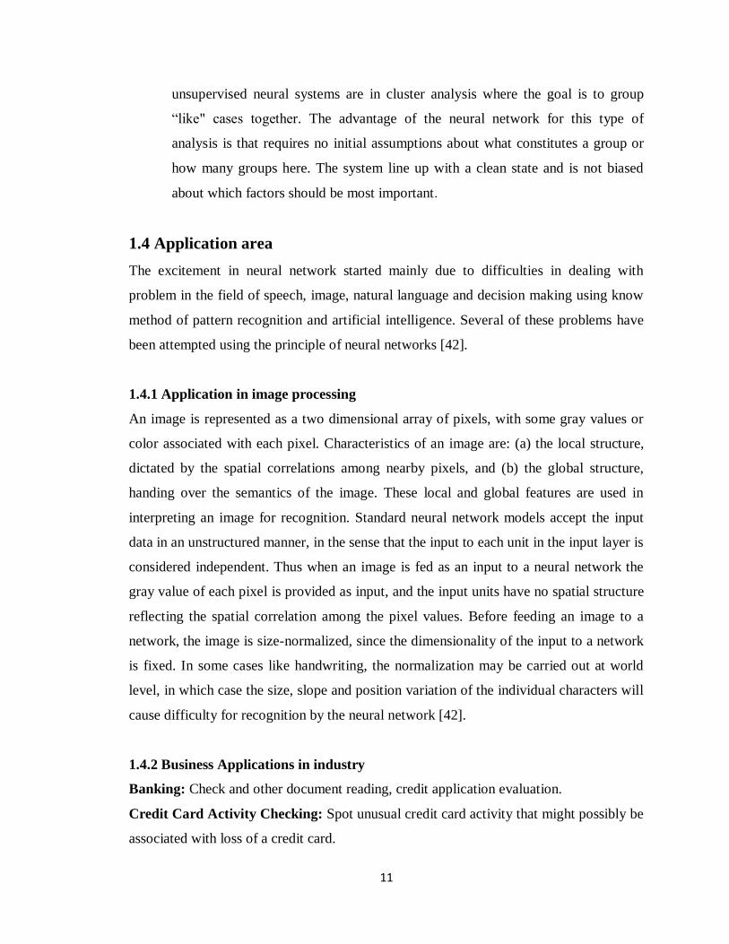
1.4 Application area
The excitement in neural network started mainly due to difficulties in dealing with
problem in the field of speech, image, natural language and decision making using know
method of pattern recognition and artificial intelligence. Several of these problems have
been attempted using the principle of neural networks [42].
1.4.1 Application in image processing
An image is represented as a two dimensional array of pixels, with some gray values or
color associated with each pixel. Characteristics of an image are: (a) the local structure,
dictated by the spatial correlations among nearby pixels, and (b) the global structure,
handing over the semantics of the image. These local and global features are used in
interpreting an image for recognition. Standard neural network models accept the input
data in an unstructured manner, in the sense that the input to each unit in the input layer is
considered independent. Thus when an image is fed as an input to a neural network the
gray value of each pixel is provided as input, and the input units have no spatial structure
reflecting the spatial correlation among the pixel values. Before feeding an image to a
network, the image is size-normalized, since the dimensionality of the input to a network
is fixed. In some cases like handwriting, the normalization may be carried out at world
level, in which case the size, slope and position variation of the individual characters will
cause difficulty for recognition by the neural network [42].
1.4.2 Business Applications in industry
Banking: Check and other document reading, credit application evaluation.
Credit Card Activity Checking: Spot unusual credit card activity that might possibly be
associated with loss of a credit card.

12
Electronics: Code sequence prediction, integrated circuit chip layout, process control,
chip failure analysis, machine vision, voice synthesis, nonlinear modeling.
Medical: Breast cancer cell analysis, EEG and ECG analysis, prosthesis design,
optimization of transplant times, hospital expense reduction, hospital quality
improvement, emergency-room test advisement.
Robotics: Trajectory control, forklift robot, manipulator controllers, vision systems.
Speech: Speech recognition, speech compression, vowel classification, text-to-speech
synthesis.
Telecommunications: Image and data compression, automated information services,
real-time translation of spoken language, customer payment processing systems.
Fig 1.11 Application areas of NN[39]
1.4.3 Application of Feed forward Neural Networks
Multilayered neural network trained using the BP algorithm account for a majority of
application of neural network to real world problem. This is because BP is easy to
implement and fast and efficient to operate. These include application domains such as:
astronomy; automatic target recognition; handwritten digit string recognition; control;

13
sonar target classification; software engineering project management; and countless
others.
1.5 Advantages of Neural Networks
Either humans or other computer techniques can use neural networks, with their
remarkable ability to derive meaning from complicated or imprecise data, to extract
patterns and detect trends that are too complex to be noticed. A trained neural network
can be thought of as an "expert" in the category of information it has been given to
analyze. Advantages include.
Adaptive learning: An ability to learn how to do tasks based on the data given for
training or initial experience.
Self-Organization: An ANN can create its own organization or representation of the
information it receives during learning time.
Real Time Operation: ANN computations may be carried out in parallel, and special
hardware devices are being designed and manufactured which take advantage of this
capability.
Fault Tolerance via Redundant Information Coding: Partial destruction of a network
leads to the corresponding degradation of performance. However, some network
capabilities may be retained even with major network damage.
1.6 Image Processing
Digital image processing means that it processing of images which are digital in nature
by a digital computer. It is motivated by three major application first one is improvement
of pictorial information for human perceptions means whatever image you get we wants
to enhance the quality of the image so that image will have better look. Second
application is for autonomous machine application this has various applications in
industry particularly for quality control and assembly automations. Third applications is
efficient storage and transmission for example if we wants to store the image on our
computer this image will need certain amount of space on our hard disk so we use some
technique so that disk space for image will required less.

14
Image processing is any form of signal processing for which the input is an images.
Digital image processing is the study of representation and manipulation of pictorial
information by a computer. Improve pictorial information for better clarity (human
interpretation). Image processing modifies pictures to improve them (enhancement,
restoration), extract information (analysis, recognition), and change their structure
(composition, image editing).
Examples:
1. Enhancing the edges of an image to make it appear sharper
2. Remove “noise” from an image
3. Remove motion blur from an image.
1.6.1 Image types
There are three type of image, which is described below [12].
Binary image: A binary image is a logical array of 0s and 1s. Pixels with the
value 0 are displayed as black; pixels with the value 1 are displayed as white.
Grayscale image: It is also known as an intensity, gray scale, or gray level
image. Array of class uint8, uint16, int16, single, or double whose pixel values
specify intensity values. For single or double arrays, values range from [0, 1]. For
uint8, values range from [0,255]. For uint16, values range from [0, 65535]. For
int16, values range from [-32768, 32767].
True color image: It is also known as an RGB image. A true color image is an
image in which each pixel is specified by three values, one each for the red, blue,
and green components of the pixel' scalar. M-by-n-by-3 array of class uint8,
uint16, single, or double whose pixel values specify intensity values. For single or
double arrays, values range from [0, 1]. For uint8, values range from [0, 255]. For
uint16, values range from [0, 65535].
15
1.6.2 Resolution
Similar to one-dimensional time signal, sampling for images is done in the spatial
domain, and quantization is done for the brightness values. In the Sampling process, the
domain of images is divided into N rows and M columns.
The region of interaction of a row and a Column is known as pixel. The value assigned to
each pixel is the average brightness of the regions. The position of each pixel is
represented by a pair of coordinates (xi, xj).
The resolution of a digital signal is the number of pixel is the number of pixel presented
in the number of columns × number of rows. For example, an image with a resolution of
640×480 means that it display 640 pixels on each of the 480 rows. Some other common
resolution used is 800×600 and 1024×728.
Resolution is one of most commonly used ways to describe the image quantity of digital
camera or other optical equipment. The resolution of a display system or printing
equipment is often expressed in number of dots per inch. For example, the resolution of a
display system is 72 dots per inch (dpi) or dots per cm.
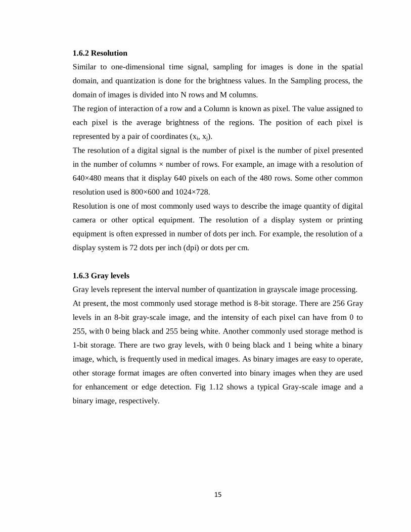
1.6.3 Gray levels
Gray levels represent the interval number of quantization in grayscale image processing.
At present, the most commonly used storage method is 8-bit storage. There are 256 Gray
levels in an 8-bit gray-scale image, and the intensity of each pixel can have from 0 to
255, with 0 being black and 255 being white. Another commonly used storage method is
1-bit storage. There are two gray levels, with 0 being black and 1 being white a binary
image, which, is frequently used in medical images. As binary images are easy to operate,
other storage format images are often converted into binary images when they are used
for enhancement or edge detection. Fig 1.12 shows a typical Gray-scale image and a
binary image, respectively.

16
(a) A Gray image (b) A Binary image
(c) Pixel image of (a) (d) Pixel image of (b)
Fig 1.12 Gray and binary image with pixel information 1.6.4 RGB Color model
In RGB color model, each colour appears in its primary spectral componets of
red,green,and blue. The color of a pixel is made up of three components; red, green, and
blue(RGB),described by there corresponding intensities. Color components are also
known as colour channels or colour planes(components). In the RGB colour model, a
colour image can be represented by the intensity function.
I RGB =(FR ,FG ,FB)
Where FR(x,y) is the intensity of the pixel (x,y) in the red channel, fG(x,y) is the intensitty
of pixel (x,y) in the green channel, and fB(x,y) is the intensity of pixel (x,y) in the blue
channel.
The intensity of each colour channel is usually stored using eight bits,which indicates that
the quantization level is 256. That is, a pixel in a colour image requires a total storage of
24 bits. A 24-bit memory can express as 224
=256×256×256=16777216 distinct colours.
The number of colours should adequately meet the display effect of most images. Such
images may be callled true colour images,where information of each pixel is- kept by

17
using a 24-bit memory.Figure 1.13 shows the images of a 24-bit colour RGB, three
channels(component) and corresponding pixel information image [12].
(a) A RGB images (b) A Pixel image of (a) (c) Red channel
(d) Pixel image of (c) (e) Green Channel (f) Pixel image of (e)
(g) Blue channel (h) Pixel image of (g)
Fig 1.13 splitting of RGB image
If only the brightness information is needed, color images can be transformed to Gray-
scale images [11] [10]. The transformation is show below in equation 1.
Iy=0.333Fr+0.5Fg+0.1666Fb ……………………………………………………..(1)

18
In RGB pixel information image there are three component(R,G,B) and each component
has a fix intensity 190, 183and 175( pixel info (1,1) in fig 1.13(b)) respectively. When
RGB image converted into Gray image then the intensity of pixel (1, 1) can be calculated
by above transformation.
Iy=0.333*190+0.5*183+0.1666*175
=183.925
In Gray pixel information image the pixel (1, 1) intensity is 184 (Shown in fig 1.12(c)).
In this way the second pixel intensity (1, 2) of Gray level image is
Iy=0.333×187+0.5×179+0.166×176
=181.15
In Gray pixel information image the pixel (1, 2) intensity is 181 (in fig 1.12(c)). In this
way we can verify all the conversation of RGB image to Gray level image with
transformation.
In RGB image the first pixel values for R, G and B is 190, 183, and 175 respectively.
RGB image split into three images (channel) R-channel, G-channel and B-channel. The
first pixel value (1, 1) of these channels is 190,183 and 175 respectively (as show above
Fig 1.13).
1.6.5 Histogram
The histogram of an image shows us the distribution of Gray levels in image massively
useful in image processing; especially in segmentation.
The array “count” can be plotted to represent a “histogram” of the image as the
number of pixels at particular gray level
The histogram can yield useful information about the nature of the image. An
image may be too bright or too dark.
It is useful to find the variations of gray levels in an image.
1.6.6 Segmentation:
Image segmentation is a process of partitioning the digital image into multiple regions
that can be associated with the properties of one or more criterion. It is an initial and vital
step in pattern recognition a series of processes aimed at overall image understanding.

19
Properties like gray level, color, texture, and shape help to identify regions and similarity
of such properties, is used to build groups of regions having a particular meaning.
Segmentation divides an image into its constituent regions or objects.
Segmentation of images is a difficult task in image processing. Still under
research.
Segmentation allows extracting objects in images.
Segmentation is unsupervised learning.
Model based object extraction, e.g., template matching, is supervised learning.
1.6.7 Image enhancement
Image enhancement improves the quality (clarity) of images for human viewing.
Removing blurring and noise, increasing contrast, and revealing details are examples of
enhancement operations. For example, an image might be taken of an endothelial cell,
which might be of low contrast and somewhat blurred. Reducing the noise and blurring
and increasing the contrast range could enhance the image [8].
Fig-1.14 (a) before enhancement Fig 1.14 (b)-after enhancement
1.6.8 Canny Edge Detection
The Canny Edge Detector is one of the most commonly used image processing tools,
detecting edges in a very robust manner. It is a multi-step process, which can be
implemented on the GPU as a sequence of filters. “Canny Edge Detection” goes over the
process of creating the canny edge detection algorithm. The algorithm detects edges
based on the pixel intensity values within a certain threshold [12].

20
1.6.9 Sobel Edge Detection
In edge detection the aim is to mark the points in a image at which the intensity changes
sharply. Sharp changes in image properties reflect important events these include: (i)
discontinuities in depth. (ii) Changes in material properties. (iii) Variations in scene
illumination. Edge detection is used in the field of image processing and feature
extraction. The Sobel operator is such an operator used edge detection algorithms [12].
In fig 1.15(a) and (b) shown canny filter and sobel filter using fig 1.12(a).
Fig-1.15 (a) After canny filter Fig 1.15(b) after sobel filter

21
Chapter 2
Review of the State of the Art / Literature Review
2.1 Survey on neural network base Face detection
Advanced image processing or computer vision techniques will enhance the quality of
symbolization of faces in video corpus. Robust face detection and tracking in videos is
still challenging. The advantage of using neural networks for face detection is the
feasibility of training a system to capture the complex class conditional density of face
patterns. However, one drawback is that the network architecture has to be extensively
tuned (number of layers, number of nodes, learning rates, etc.) to get exceptional
performance. Many research efforts have been made in face detection, especially for
surveillance and biometrics. In a comprehensive survey for face detection is presented. In
addition to face detection and recognition, behavior analysis is also helpful, especially to
associate the behavior with person‟s activity described in text. There are some major face
detection approach on the bases of minimal size of input image and the features.
Table 2.1 surveys on Face detection
Authors Year Approach Features Used Head
Pose
Test database Minimal
Face Size
N.
Huijsmans
[16]
1996 Markov Random
Field DFFS
Most
informative
pixel
Frontal MIT; CMU,
Leiden
23×32
R. Cipolla
[17]
1997 Feature Belief
networks
Geometrical
facial features
Frontal
to profile
CMU 60×60
T. S. Huang
[18]
1997 Learning Markov
process
Frontal FERET 11×11
T. Poggio
[19]
Learning Texture Frontal Mug shots
CCD pictures;
newspaper
scans FERET
19×19
N. Ahuja
[20]
1998 Multiscale
segmentation;
color model
Skin color
intensity
Texture
Frontal Color pictures NA

22
S. Baluja
[21][22]
1998 Neural network Texture Frontal CMU; FERET;
Web images
20×20
G. Garcia
[23]
1999 Statistical Wavelet
analysis
Color;
wavelets
coefficients
Frontal
to near
frontal
MPEG videos 80×48
Q. Chen
[24]
1999 Fuzzy color
models; Templates
matching
Color Frontal
to profile
still color
images
20×24
D. Maio
[25]
2000 facial templates
Hough
Transformation
Texture;
Directional
images
Frontal Static images 20×27
R. Feraud
[26]
2001 Neural network Motion, color,
Texture
Frontal
and
profile
Sussex CMU:
web page
15×20
In 2002[27] Rein-Lien Hsu, Mohamed Abdel-Mottaleb, and Anil K. Jain proposed a face
detection algorithm for color image in which two modules are contain. In first modules
face localization for finding face candidates and in second modules facial feature
detection for verifying detected face candidate. The facial feature detection modules
rejected face candidate regions that do not contain any facial feature such as eyes, mouth
and face boundary map done and finally we utilize the hough transform to extract the best
fitting ellipse. Their system arbitrates between multiple networks to improve performance
over a single neural network. Capable of correctly locating upright frontal faces in gray
level images, the detector proved to perform well with varying lighting conditions, and
relatively complex backgrounds. Presented here is a summary of the detector, its unique
features, and an evaluation of its performance.
In 2003 [28] Ragini Choudhury Verma, Cordelia Schmid, and Krystian Mikolajczyk
proposed a theory on Face Detection and Tracking in a Video by Propagating Detection
Probabilities. The proposed algorithm is divided into two phases, first phase is detection
and second phase is prediction and update tracking. In first phase, detects the regions of
interest that potentially contain faces. A detection probability is associated with each
pixel, for different scales and two different views, one for frontal and one for profile

23
faces. This phase also identifies the detection parameters that characterize the face
position, scale, and pose. These parameters can be computed using frame-by-frame
detection. However, the detector response can decrease due to different reasons
(occlusions, lighting conditions, face pose) and depends on a threshold. In second phase,
we use a Condensation filter and factored sampling to propagate the detection parameters
over time and, hence, track the faces through the video sequence. Experiments have been
carried out on video sequences with multiple faces in different positions, scales (sizes),
and poses, which appear or disappear from the sequence. We have applied the two
approaches to 24 sequences (4,650 faces in 3,200 frames). We used a threshold of 0.7 for
frame-based detection, which was empirically found to be optimal. The thresholds of the
temporal detector are the ones presented previously. The results of the comparison with
respect to false detections and missing detections are 3(0.065%) and 40 for temporal
approach and 558(12%) and 368 respectively. The percentage-missing detections are
computed with respect to the total number of faces. We can see that the temporal
approach performs much better than the frame-based detection however; a few failure
cases remain in the case of the temporal approach.
In 2004[29] Stefan Wiegandy, Christian Igely and Uwe Handmann proposed an
evolutionary algorithm for face detection. In evolutionary network optimization the goal
of the optimization is to reduce the number of hidden nodes of the detection network
under the constraint that the classification error does not increase. We tolerate an increase
in the number of connections as long the number of neurons decreases. We initialize our
optimization algorithm and compare our results with the expert-designed architecture.
The speed of classification whether an image region corresponds to a face or not could be
improved by approximately 30 %.
In 2005 [30]Yuehui Chen, Shuyan Jiang, and Ajith Abraham presented a theory on face
recognition using DCT and hybrid flexible neural tree classification model. DCT has
some fine properties i.e. de-correlation energy compaction, separability, symmetry and
orthogonality DCT coefficient matrix of an image covering all the spatial frequency
components of the images. The DCT convert high-dimensional face image into low

24
dimensional space in which more significant facial feature such as outline of hair and
face position of eye, nose and mouth are maintained. FNT model is union of function set
(F) and terminal instruction set T and the end give the comparison result between
different approach for e.g. Principal Component Analysis (PCA) and RBFN (Radial
Basic Function Network), LDA (Linear Discriminant analysis) and RBFN, FS and RBFN
and last approach is DCQ and FNT. The size of input image should be 92×112.
In 2006 [31]Uma D. Nadimpalli, Randy R. Price, Steven G. Hall, and Pallavi Bomma
presented a theory for bird recognition on the base of template matching. First all the
images divide into three types of images, in first type of images were very clear, in
second type images were medium clear and third type image were unclear. Neural
network architecture has 5 neurons in hidden layer and one neuron in output layer and
130×100 neuron in the input layer. There is no rule to calculate the optimum number of
element in the hidden layer. We preset the target values for the bird and non-bird picture
at 0.9 and 0.1. Input image of size 130×100 have been trained. ANN obtained accuracies
of 100, 60 and 50% on type-1, type-2, and type-3 image respectively. Type 1 images
obtained high accuracies because these images were clear and training became easy.
Type 2 and Type 3 images obtained low accuracies because some images had birds,
which were small, and some images contained birds that were not clear due to the
movement of the platform while using the camera. Image morphology using HSV color
space worked well on all types of images compared to other color spaces. ANN has
worked better on Type 1 images than Type 2 and Type 3 images. Accuracies in these
cases can be improved by proper training of images. Template matching worked well and
produced high accuracy rates.
In 2006 [32] Jean Choi, Yun-Su Chung, Ki-Hyun Kim, and Jang Hee Yoo presented a
theory on face recognition which are based on DCT(Discrete Cosine Transform),
EP(Energy Probability) and LDA(Linear Discrimirant Analysis). In given block diagram
of proposed method there are three step in first step images is transformed into frequency
domain, second Energy probability (EP) it is applied on DCT domain which acquires
from face images dimension reduction of data and optimization of valid information. The

25
energy is one of the image properties using signal-processing technique, and it means
characteristics of images. And last LDA (Linear Discrimirant Analysis) it is applied to
extracted data using frequency mask. And the last compared the result from the following
feature extraction methods: (a) PCA plus LDA, (b) existing DCT method, and (c)
proposed method. The best recognition rates of PCA plus LDA, existing DCT method,
and proposed method are 90.0%, 94.4%, and 96.8%, respectively. The image size should
be 64×64.
In 2007[33] Abdallah S. Abdallah, A.Lynn Abbott, and Mohamad Abou El-Nasr proposed
a theory for face detection using 2D discrete cosine transform (DCT) and self-organizing
feature map (SOM). DCT used for feature extracted and supervised SOM training session
is used to cluster feature vector into groups, and to assign “face”, or “non-face” labels to
those clusters. In the first stage we use color base segmentation (find out the interested
area on the base of color). The size of segmented image should be 300×255. In second
stage we analysis the region and labeled them. The segmented image divided region into
block size 32×32 pixels. In third stage DCT chosen which are used for feature extraction
and for block size 16×16 a total 256 DCT coefficient were computed for each sample.
Fourth stage is SOM neural network if face presented then detected using a self-
organizing map. The system has been tested using a sizable database containing 1027
faces in many orientations, sizes, and skin colors, and it achieved a detection rate of
77.94% during subsequent tests with false positive rate of 5.14%.
In 2008 [34] Wang Zhanjie and Tong Li proposed a method for face detection based on
skin color and neural network. There are two steps in first step the face-like regions are
segmented based on the features of human face color. For skin color segmented we used
color space YCrCb that is a hardware-oriented color model. Y represents the luminance
component, while Cr and Cb represent the chrominance components of an image. In
second stage neural network based face detection in gray image, which provide a simple
yet effective approach for learning of a nonlinear classification function, not only is used
to select features, but also is used to classy face and no face. Face detection is a
dichotomize mission, so output of neural network is a 2-dimension vector. Define face as
26
(1, 0) and non-face as (0, 1). The proposed detection method have lower detection rate
than others. Detection rate (70.2 %) of proposed methods is lower than Viola-Jones‟
(76.1 %).
In 2009 [3]Zahra Sadri Tabatabaie, Rahmita Wirza Rahmat, Nur Izura Binti Udzir and
Esmaeil Kheirkhah presented a theory of face detection system using combination of
appearance-based and Feature-based methods and also compared with the result of Viola
and jones face detection method with a color base method. zahra improves the
performance of face detection system in term of increasing the face detection speed and
decreasing false positive rate. In this approach, first skin regions in the input image are
identified using above mentioned method ((R, G, B) is classified as skin if: R > 95 and G
> 40 and B > 20 and Max{R, G, B} −Min{R, G, B} > 15 and |R−G| > 15 and R > G and
R > B) and then Viola and Jones algorithm is applied for detecting faces. After applying
skin color classifier, all non-skin regions replace with black, whereas skin regions remain
stationary. This helps face detection algorithm to quickly identify non-faces, which
include majority pixels of each image. Also this method efficiently reduces false positive
rate. The accuracy is 77.14%, false positive rate 5.44 and false negative rate 17.42%.
2.2. Techniques
Techniques for face detection in image are classified into four categories.
2.2.1. Knowledge based method
It is dependent on using the rules about human facial features. It is easy to come up with
simple rules to describe the features of a face and their relationships. For example, a face
often appears in an image with two eyes that are symmetric to each other, a nose, and a
mouth, and features like relative distance and position represent relationships between
features. After detecting features, verification is done to reduce false detection. This
approach is good for frontal image; although the difficulty is how to translate human
knowledge into known rules and to detect faces in different poses [2].

27
2.2.2 Image Based method:
In this approach, there is a predefined standard face pattern, which is used to match with
the segments in the image to determine whether they are faces, or not. It uses training
algorithms to classify regions into face or non-face classes. Image-based techniques
depends on multi-resolution window scanning to detect faces, so these techniques have
high detection rates but slower than the feature-based techniques. Eigen-faces and neural
networks are examples of image-based techniques.
2.2.3 Features Based method
In feature-based approaches researchers have been trying to find invariant features of
faces for detection. The underlying assumption is based on the observation that humans
can effortlessly detect faces and objects in different poses and lighting conditions and, so,
there must exist properties or features (such as eyebrows, eyes, nose, mouth, and skin
color) which are invariant over these variability‟s. Numerous methods have been
proposed to first detect facial features and then to infer the presence of a face. Based on
the extracted features, a statistical model is built to describe their relationships and to
verify the existence of a face. In this paper skin color feature will be discussed and used
[3].
2.2.4 Template matching method
Template matching is performed first to find the regions of high correlation with the face
and eyes templates. Subsequently, using a mask derived from color segmentation and
cleaned by texture filtering and various binary operations, the false and repeated hits are
removed from the template matching result. The basic idea of template matching is to
convolve the image with another image (template) that is representative of faces.
Template matching is a method of comparing an input image with a standard set of
images known as templates. Templates are face parts cut from various pictures. Normal
correlation between the input image and each template image is calculated. This
technique compares two images to decide if the desired shape was being viewed [35]
[15]. Template matching methods use the correlation between pattern in the input image
and stored standard patterns of a whole face / face features to determine the presence of a

28
face or face features. Predefined templates as well as deformable templates can be used.
A template-based face detection method includes: producing an average face image from
a face database, wavelet-converting the produced face image, and removing a low
frequency component of high and low frequency components of the converted image, the
low frequency component being sensitive to illumination; producing a face template with
only high horizontal and vertical frequency components of the high frequency
components; and retrieving an initial face position using the face template when an image
is inputted, and detecting the face in a next frame by using, as a face template for the next
frame, a template obtained by linearly combining the face template with a high frequency
wavelet coefficient corresponding to the position of the face in a current frame. Thus, the
method has a shortened calculation time for face detection, and can accurately detect a
face irrespective of skin color and illumination [2].

29
Chapter 3
Problem Statement and Methodology
Problem statement describes the gap in the existing work and problem formulation. The
Gap in existing work shows, what are the limitation in the existing work and which
technique they are used. In problem formulation, we give appropriate solution to solve
the existing problem and suggest the novel work.
3.1 Problem Statement
Detecting human faces in images is a challenging problem in computer vision, and is a
hot topic of research in both commercial and academic institutions throughout the world.
Face detection is the most important part of face identification and it is difficult due to
varying of illumination, pose of head and face expression Human face detected in an
image can represent the presence of a human in a place. Evidently, face detection is the
first step towards creating an automated system, which may involve other face
processing. Differences between face detection and other face processing have been
explained, as given by the following:
Face detection: To determine if there is any face in an image.
Face localization: To locate position of a face in image.
Face tracking: To continuously detect location of a face in image sequence in
real-time.
Face recognition: To compare an input image against the database and report a
match if similar.
Face authentication: To verify the claim of the identity by an individual in a
given input image.
Facial expression recognition: To identify the states/ emotion of a human based
on face evaluation.
Facial feature detection: To detect presence and location of face features.
Face detection is an active area of research spanning disciplines such image processing,
pattern recognition and computer vision. Face detection and recognition are preliminary
steps to wide of applications such as personal identity, video surveillance etc. the

30
detection efficiency influences the performance of these systems, there have been various
approaches for face detection, which classified into four categories (i) knowledge based
method (ii) feature based method (iii) template matching method (iv) appearance based
method.
In face detection applications, face usually form an inconsequential region of images.
Consequently, preliminary segmentation of images into regions that contain "non-face"
objects and regions that may contain "face" candidates can greatly accelerate the process
of human face detection.
NN based methods require a large number "face" and "non-face" images to train the
neural network for getting the network model.
A key question in face detection is how to best discriminate faces from non-face
background images. However, for realistic situations, it is very difficult to define a
discriminating metric because human faces usually vary strongly in their appearance due
to ethnic diversity, expressions, poses, and aging, which makes the characterization of the
human face difficult. Furthermore, environmental factors such as imaging devices and
illumination can also exert significant influences on facial appearances. In the past
decade, extensive research has been carried out on face detection, and significant
progress has been achieved to improve the detection performance with the following two
performance goals.
3.2 Motivation
Face detection plays an important role in today‟s world. They have many real world
applications like human/computer interface, surveillance, authentication and video
indexing. However research in this field is still young.
The Face detection system can benefit the areas of: Law Enforcement, Airport Security,
Access Control, Driver's Licenses & Passports, Homeland Defense, Customs &
Immigration and Scene Analysis. The following paragraphs detail each of these topics, in
turn. In face recognition the first step is face detection so these topics are related face
recognition as well as face detection.
Law Enforcement: Today's law enforcement agencies are looking for innovative
technologies to help them stay one step ahead of the world's ever-advancing terrorists.

31
Airport Security: It can enhance security efforts already underway at most airports and
other major transportation hubs (seaports, train stations, etc.). This includes the
identification of known terrorists before they get onto an airplane or into a secure
location.
Access Control: It can enhance security efforts considerably. Biometric identification
ensures that a person is who they claim to be, eliminating any worry of someone using
illicitly obtained keys or access cards.
Driver's Licenses & Passports: It can leverage the existing identification infrastructure.
This includes, using existing photo databases and the existing enrollment technology (e.g.
cameras and capture stations); and integrate with terrorist watch lists, including regional,
national, and international "most-wanted" databases.
Homeland Defense: It can help in the war on terrorism, enhancing security efforts. This
includes scanning passengers at ports of entry; integrating with CCTV cameras for "out-
of-the-ordinary" surveillance of buildings and facilities; and more.
Customs & Immigration: New laws require advanced submission of manifests from
planes and ships arriving from abroad; this should enable the system to assist in
identification of individuals who should, and should not be there [36].
3.3 Methodology
The step-by-step methodology followed for face detection in given image using soft
computing technique (image processing and neural network) is as follows:
Define the neural network architecture.
Uses of transformation (FFT and DCT).
Gabor filters for Feature Extraction.
Chose the neural network architecture parameter.
Train the neural network (FFNN).
Testing the image

32
Chapter 4
Implementation of Face Detection Algorithm
This chapter includes detail of implementation the face detection algorithm. MATLAB
7.5 R2007b was used for the implementation of various algorithms. It integrates
computation, visualization and programming in easy to use environment. As discussed in
the Literature Survey, there are many different approaches to face detection, each with
their own relative merits and limitations. One such approach is that of Neural Networks.
This section gives a brief introduction to the theory of neural networks and presents a
neural network-based face detector.
4.1 What Is MATLAB
The name MATLAB stands for MATrix LABoratory.
Dr. Cleve Moler, chief scientist at Math Works Inc. originally wrote MATLAB to
provide easy access to matrix software developed in the LINPACK and EISPACK
projects. The first version was written in the late 1970s for the use in courses in matrix
theory, linear algebra, and numerical analysis. MATLAB is therefore built upon a
foundation of sophisticated matrix software, in which the basic data element is a matrix
that does not require predimensioning. MATLAB is a product of the Math Works, Inc.
and is an advanced software package specially designed for scientific and engineering
computation. MATLAB is a high-performance language for technical computing [1]. It
integrates computation, visualization, and programming in an easy-to-use environment
where problems and solutions are expressed in familiar mathematical notation. MATLAB
is an interactive system whose basic data element is an array that does not require
dimensioning. This allows you to solve many technical computing problems, especially
those with matrix and vector formulations, in a fraction of the time it would take to write
a program in a scalar non-interactive language such as C or FORTRAN. MATLAB has
evolved over a period of years with input from many users. In university environments, it
is the standard instructional tool for introductory and advanced courses in mathematics,
engineering, and science. In industry, MATLAB is the tool of choice for high-

33
productivity research, development, and analysis. The reason that I have decided to use
MATLAB for the implemented some algorithms, which are related the thesis work.
Toolboxes allow you to learn and apply specialized technology. Toolboxes are
comprehensive collections of MATLAB functions (M-files) that extend the MATLAB
environment to solve particular classes of problems [1].
4.2 Neural Network Toolbox
The neural network toolbox makes it easier to use neural networks in matlab. The toolbox
consists of a set of functions and structures that handle neural networks, so we do not
need to write code for all activation functions, training algorithms, etc. that we want to
use.
4.2.1 Introduction to the GUI
The graphical user interface (GUI) is designed to be simple and user friendly. Once the
Network/Data Manager window is up and running, you can create a network, view it,
train it, simulate it, and export the final results to the Workspace. Similarly, you can
import data from the workspace for use in the GUI. It goes through all the steps of
creating a network and shows what you might expect to see as you go along.
4.2.2 Create a neural Network (nntool):
Create a neural network to perform the specific task. It has an input vector and a target
vector. Call the network Net. Once created, the network will be trained. You can then
save the network, its output, etc., by exporting it to the workspace.
4.2.3 Input and Target
To start, type nntool on MATLAB main window. The following window appears.

34
Fig 4.1 nntool (data manager)
First, define the network input, called data 1. To define this data, click New, and a new
window, Create Network or Data, appears. Select the Data tab. Set the Name to data1,
and make sure that Data Type is set to inputs.
Fig 4.2 Create network
Click Create and then click OK to create an input data1. The Network/Data Manager
window appears, and data1 shows as an input. Next create a network target. This time
enter the variable name data 2, and click Target under Data Type. Again click Create and
OK. You will see in the resulting Network/Data Manager window that you now have
data2 as a target as well as the previous data1 as an input.

35
4.2.4. Create Network:
Now create a new network. Select the Network tab. Set the Network Type to feed
forward back prop, for that is the kind of network you want to create. You can set the
inputs to data1, and the targets to data2. You can use a tansig transfer function with the
output range [-1, 1] that matches the target values and a learngd learning function. For the
training function, select traincgb or trainscg. For the Performance function, select msereg.
The Create Network or Data window now looks like the following figure.
Fig 4.3Create network to examine the network
click View.
Fig 4.4 network viewer

36
This is the desired neural network. Now click Create and OK to generate the network.
Now close the Create Network or Data window. You see the Network/Data Manager
window with Network1 listed as a network.
4.2.5. Train the Neural network
To train the network, click Network 1 to highlight it. Then click Open. This leads to a
new window, labeled Network: network1. At this point you can see the network again by
clicking the View tab. You can also check on the initialization by clicking the Initialize
tab. Now click the Train tab, specify the inputs and output by clicking the Training Info
tab and selecting data 1 from the list of inputs and data 2 from the list of targets. The
Network: network1window should look like Note that the contents of the Training
Results Outputs and Errors fields have the name network1 prefixed to them. This makes
them easy to identify later when they are exported to the workspace. While you are here,
click the Training Parameters tab. It shows you parameters such as the epochs and error
goal. You can change these parameters at this point if you want. Click Train Network.
Training with TRAINSCG window appears.
Fig 4.5 Train network
4.3 Performance Functions
In MATLAB, there are many function for performance of neural network for e.g. mae
(Mean absolute error performance function), mse(Mean squared error performance
function), msne(Mean squared normalized error performance function), msnereg(Mean

37
squared normalized error with regularization performance functions)and msereg(Mean
squared error with regularization performance function). Everyone has some special
feature but according to the problem statement „msereg‟ function are used for
performance of neural network so discussed only msereg function.
4.3.1 Description of msereg:
msereg is a network performance function. It measures network performance as the
weight sum of two factors:
The mean squared error and the mean squared weight and bias values.
msereg(E,Y,X,FP) takes E and optional function parameters,
E Matrix or cell array of error vectors
Y Matrix or cell array of output vectors (ignored)
X Vector of all weight and bias values
FP.ratio Ratio of importance between errors and weights
and returns the mean squared error plus FP.ratio times the mean squared weights.
Network Use
You can create a standard network that uses msereg with newff, newcf, or newelm. To
prepare a custom network to be trained with msereg, set net.performFcn to 'msereg'. This
automatically sets net.performParam to msereg's default performance parameters.
In either case, calling train or adapt results in msereg's being used to calculate
performance.
4.4 Training Functions
In MATLAB there are many function for trained the neural network for e.g.
trainbfg(BFGS quasi-Newton backpropagation), traincgb(Powell-Beale conjugate gradi-
ent backpropagation), traincgf(Fletcher-Powell conjugate gradient backpropagation),
traincgp (Polak-Ribiére conjugate gradient backpropagation), traingd(Gradient descent
backpropagation), traingda(Gradient descent with adaptive learning rule backpropa-
gation), traingdm(Gradient descent with momentum backpropagation), traingdx(Gradient
descent with momentum and adaptive learning rule backpropagation),trainlm(Levenberg
Marquardt backpropagation), trainoss(One step secant backpropagation), trainrp(Resilient

38
backpropagation), trainscg(Scaled conjugate gradient backpropagation). But according to
the problem statement training function „trainscg‟ and „traincgb‟ are used for train the
neural network, so discuss only two training function here.
4.4.1 Description of trainscg
„trainscg‟ is a network training function that updates weight and bias values according to
the scaled conjugate gradient method [41]
trainscg (net,Pd,Tl,Ai,Q,TS,VV,TV) takes these inputs,
net Neural network
Pd Delayed input vectors
Tl Layer target vectors
Ai Initial input delay conditions
Q Batch size
TS Time steps
VV Either an empty matrix [] or a structure of validation vectors
TV Either an empty matrix [] or a structure of test vectors
And returns
net Trained network
TR Training record of various values over each epoch:
TR.epoch Epoch number
TR.perf Training performance
TR.vperf Validation performance
TR.tperf Test performance
Ac Collective layer outputs for last epoch
El Layer errors for last epoch
Network Use
You can create a standard network that uses trainscg with newff, newcf, or newelm. To
prepare a custom network to be trained with trainscg, Set net.trainFcn to 'trainscg'. This
sets net.trainParam to trainscg's default parameters. Set net.trainParam properties to
desire values. In either case, calling train with the resulting network trains the network
with trainscg.

39
4.4.2 Description of Traincgb
„traincgb‟ is a network training function that updates weight and bias values according to
the conjugate gradient backpropagation with Powell-Beale restarts[13]. traincgb can train
any network as long as its weight, net input, and transfer functions have derivative
functions. Backpropagation is used to calculate derivatives of performance perf with
respect to the weight and bias variable [41].
traincgb(net,Pd,Tl,Ai,Q,TS,VV,TV) takes these inputs,
net Neural network
Pd Delayed input vectors
Tl Layer target vectors
Ai Initial input delay conditions
Q Batch size
TS Time steps
VV Either an empty matrix [] or a structure of validation vectors
TV Either an empty matrix [] or a structure of test vectors
and returns
net Trained network
TR Training record of various values over each epoch:
TR.epoch Epoch number
TR.perf Training performance
TR.vperf Validation performance
TR.tperf Test performance
Ac Collective layer outputs for last epoch
El Layer errors for last epoch
Network Use
You can create a standard network that uses traincgb with newff, newcf, or newelm.
To prepare a custom network to be trained with traincgb,
1. Set net.trainFcn to 'traincgb'. This sets net.trainParam to traincgb's default
parameters.
2. Set net.trainParam properties to desire values [13].
In either case, calling train with the resulting network trains the network with traincgb.

40
4.5 Layer Initialization Functions
In MATLAB there are many function for trained the neural network for e.g initnw
(Nguyen-Widrow layer initialization function), initwb(By-weight-and-bias layer
initialization function), initlay(layer-by-layernetwork initialization function). But in our
neural network architecture used only „initlay‟ function for initialization the layer of
neural network. So discuss only „initlay‟ function here [41]
4.5.1 Description of Initlay
„Initlay‟ is a network initialization function that initializes each layer i according to its
own initialization function net.layers{i}.initFcn. initlay(net) takes net Neural network and
returns the network with each layer updated. initlay(code) returns useful information for
each code string:
'pnames' Names of initialization parameters
'pdefaults' Default initialization parameters
initlay does not have any initialization parameters.
Network Use
You can create a standard network that uses initlay by calling newp, newlin, newff,
newcf, and many other new network functions.
To prepare a custom network to be initialized with initlay,
1. Set net.initFcn to 'initlay'. This sets net.initParam to the empty matrix [],
because initlay has no initialization parameters.
2. Set each net.layers{i}.initFcn to a layer initialization function. (Examples
of suchfunctions are initwb and initnw.)
To initialize the network, call init.
4.6 Image Processing Toolbox
Image Processing Toolbox is a collection of functions that extend the capability of the
MATLAB numeric computing environment. The toolbox supports a wide range of image
processing operations. In this thesis work, we have used image-processing toolbox of
MATLAB 7.5 R2007.
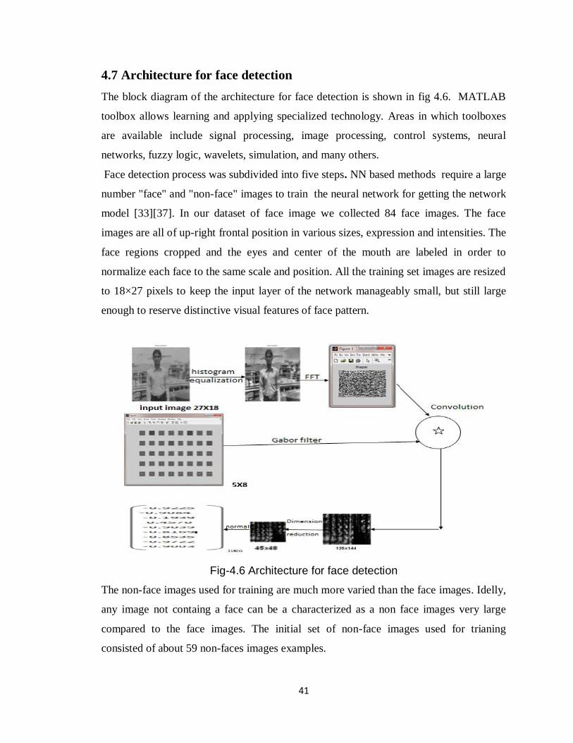
41
4.7 Architecture for face detection
The block diagram of the architecture for face detection is shown in fig 4.6. MATLAB
toolbox allows learning and applying specialized technology. Areas in which toolboxes
are available include signal processing, image processing, control systems, neural
networks, fuzzy logic, wavelets, simulation, and many others.
Face detection process was subdivided into five steps. NN based methods require a large
number "face" and "non-face" images to train the neural network for getting the network
model [33][37]. In our dataset of face image we collected 84 face images. The face
images are all of up-right frontal position in various sizes, expression and intensities. The
face regions cropped and the eyes and center of the mouth are labeled in order to
normalize each face to the same scale and position. All the training set images are resized
to 18×27 pixels to keep the input layer of the network manageably small, but still large
enough to reserve distinctive visual features of face pattern.
Fig-4.6 Architecture for face detection
The non-face images used for training are much more varied than the face images. Idelly,
any image not containg a face can be a characterized as a non face images very large
compared to the face images. The initial set of non-face images used for trianing
consisted of about 59 non-faces images examples.

42
Step 1:
4.8 Histogram equalization
As the low-contrast image‟s histogram is narrow and centered toward the middle of the
gray scale, if we distribute the histogram to a wider range the quality of the image will be
improved. It transforms the intensity values so that the histogram of the output image
approximately matches the flat (uniform) histogram [12]. We are using Contrast-limited
adaptive histogram equalization (CLAHE) method for histogram equalization.
Syntax
J = adapthisteq(I)
Description J = adapthisteq(I) enhances the contrast of the grayscale image I by
transforming the values using contrast-limited adaptive histogram equalization
(CLAHE).CLAHE operates on small regions in the image, called tiles, rather than the
entire image. Each tile's contrast is enhanced, so that the histogram of the output region
approximately matches the histogram specified by the 'Distribution' parameter. The
neighboring tiles are then combined using bilinear interpolation to eliminate artificially
induced boundaries. The contrast, especially in homogeneous areas, can be limited to
avoid amplifying any noise that might be present in the image [7].
Step 2:
4.9 Transformation
After applying histogram equalization with input image of size 18x27 we apply the
Fourier transformation FFT (and DCT) for feature extraction. The image after Fourier
Transformation is shown in fig 4.7(b).
Y =fft2(X) returns the two-dimensional discrete Fourier transform (DFT) of X, computed
with a fast Fourier transform (FFT) algorithm. The result Y is the same size as X .

43
Fig 4.7(a) input image Fig 4.7(b) After FFT Fig 4.8(c) After DCT
Fig-4.7 Image before and after FFT and DCT
The image after discrete cosine Transformation is shown in below fig 4.7. The discrete
cosine transformation (DCT) represents an image as a sum of sinusoids of varying
magnitudes and frequencies. The dct2 function computes the two-dimensional discrete
cosine transform (DCT) of an image (third image of Fig 4.7). The DCT has the property
that, for a typical image, most of the visually significant information about the image is
concentrated in just a few coefficients of the DCT. For this reason, the DCT is often used
in image compression applications.
Step-3:
4.10 Gabor filters
A Gabor filter is a linear filter whose impulse response is defined by a harmonic function
multiplied by a Gaussian function.
Because of the multiplication-convolution property (Convolution theorem), the Fourier
transform of a Gabor filter's impulse response is the convolution of the Fourier transform
of the harmonic function and the Fourier transform of the Gaussian function.
A Gabor filter can be applied to images to extract feature aligned at particular orientation.
Gabor filters posses the optimal localization properties in both spatial and frequency
domains, and they have been successfully used in many applications. A Gabor filter is a
function obtained by modulating a sinusoidal with a Gaussian function. The useful
parameters of a Gabor filter are orientation and frequency. The Gabor filter is thought to
mimic the sample cells in the visual cortex [21]. In our case a Gabor filter bank is

44
implemented on face images with 8 different orientation and 5 different frequencies (in
Fig 4.8).
Fig 4.8 Gabor filter of 5 frequencies and 8 orientations
Gabor wavelet transformation is done by convolution of the image with the 40 Gabor
filters shown in figure 4.8 above.
Formally the Gabor filter is a Gaussian (with variances Sx and sy along x and y-axes
respectively) and is described by the Equation 2:
……………… (2)
Sx & Sy: Variances along x and y-axes respectively
U x& Vy: Centre frequencies along x and y-axes respectively
G: The output filter as described above
The variance terms Sx and Sy dictates the spread of the band pass filter centered at the
frequency U and V in the frequency domain. This filter is complex in nature.
A Gabor filter can be described by the following parameters: the Sx and Sy of the
Gaussian explain the shape of the base (circle or ellipse), frequency (f) of the sinusoid,
orientation (Ө) of the applied sinusoid. Fig 4.8 show example of Gabor filters [7].
A 27×18 images is transformed to size 27×18×5×8. Thus the feature vector consists of all
useful information extracted from different frequencies, orientation and from all location,
and hence is very useful for expression recognition.
The representation of facial feature is based on Gabor wavelet transform. Gabor wavelets
are biologically motivated convolution kernels in the shape of plane waves restricted by a

45
Gaussian envelope function. We use the Gabor wavelet because it can extract the human
face feature well.
When the size of image (27×18) convolution with the Gabor filter (5×8), it becomes
145×144 but due to large size (or large number of input in neural network) we reduce the
dimensions from 145×144 to 45×48. And then Convert cell array of matrices to single
matrix 2160×1 using cell2mat() function. This single matrix goes to as a input in neural
network means that number of input in neural network is 2160(neurons) for a single input
image. In fig 4.10 pixel info is given at the left bottom (1, 2160) -0.98. It means the last
pixel intensity is -0.98 and pixel co-ordinate is (1, 2160).
Fig 4.9 Input image with different orientations Fig 4.10 Single matrix of input image
Step-4:
4.11 Selection of network architecture
Both the generalization and approximation ability of a feed forward neural network are
closely related to the network and the size of the training set. The really problem is to
find a network architecture that is capable of approximation and generalization
simultaneously.
4.11.1 How Many Hidden Layers are enough
When we say three layered we imply a structure input-hidden-output. The problem with
multilayer networks using a single hidden layer is that the neurons tend to interact either

46
each other globally. Neurons in the first hidden layer learn the local features that
characterize specific region of the input space. For example, in the optical character
recognition network of Sackinger [39] the network uses a five-layered architecture.
4.11.2. How Many Hidden Neurons are enough
The problem of selecting the number of neurons in the hidden layers of multilayer of
networks is an important issue that remains open for research. The number of nodes must
be large to form a decision regions as complex as that required by the problem. And yet
the number must not be excessively large so that weights cannot be reliably estimated by
available training data.
We have already discussed in the section 4.3, 4.4 and 4.5, there was lot of function for
training, performance, transfer, and initialization of neural network layer but according to
problem statement some function selected and apply them with the problem statement.
Layer Initialization Functions: initlay
Performance Functions: msereg
Training Functions: trainscg (and traincgb)
Transfer function: tansig
Using all these function made a feed forward neural network take a snap shot with the
help of MATLAB 7.5, which are shown below. There are 2160 input neuron in input
layer, which already discuss in step 3 and single hidden layer was used.
In hidden layer 100 neurons (in Fig 4.11) are present for storage the weight value of
given input. The overall architecture of your neural network is store in the variable „net‟.
Fig 4.11 Neural network architecture with 100 hidden neurons

47
Step-5
4.12 Training algorithm and image testing
Fig 4.12 Finalization of Face locator using template matching
The training process requires a set of face and non-face folder of fix size. During training
process our goal is 0.001 and epochs set on maximum 400. We divided training process
into four categories to find the better solution of our problem.
Training with FFT and trainscg (FFT_TRAINSCG).
Training with DCT and trainscg (DCT_TRAINSCG).
Training with FFT and triancgb (FFT_TRAINCGB).
Training with DCT and traincgb (DCT_TRAINCGB).
Testing of images are based on template matching we chose two template face image
(template1.jpf, template2.jpg). Template matching involves convolving the image with
some template.
Once individual candidate face images are separated, template matching is used as not
only a final detection scheme for faces, but also for locating the centroid of the face (in
Fig 4.12). The idea of template matching is to perform cross-co variances with the given
image and a template that is representative of the image [35][15]. Therefore, in
application to face detection, the template should be a representative face - being either
an average face of all the faces in the training images, or an eigenface. In our case, both
templates were created. The first step was to crop out the faces from each training image
posted on the website. Using these faces as our set of training images was justified since
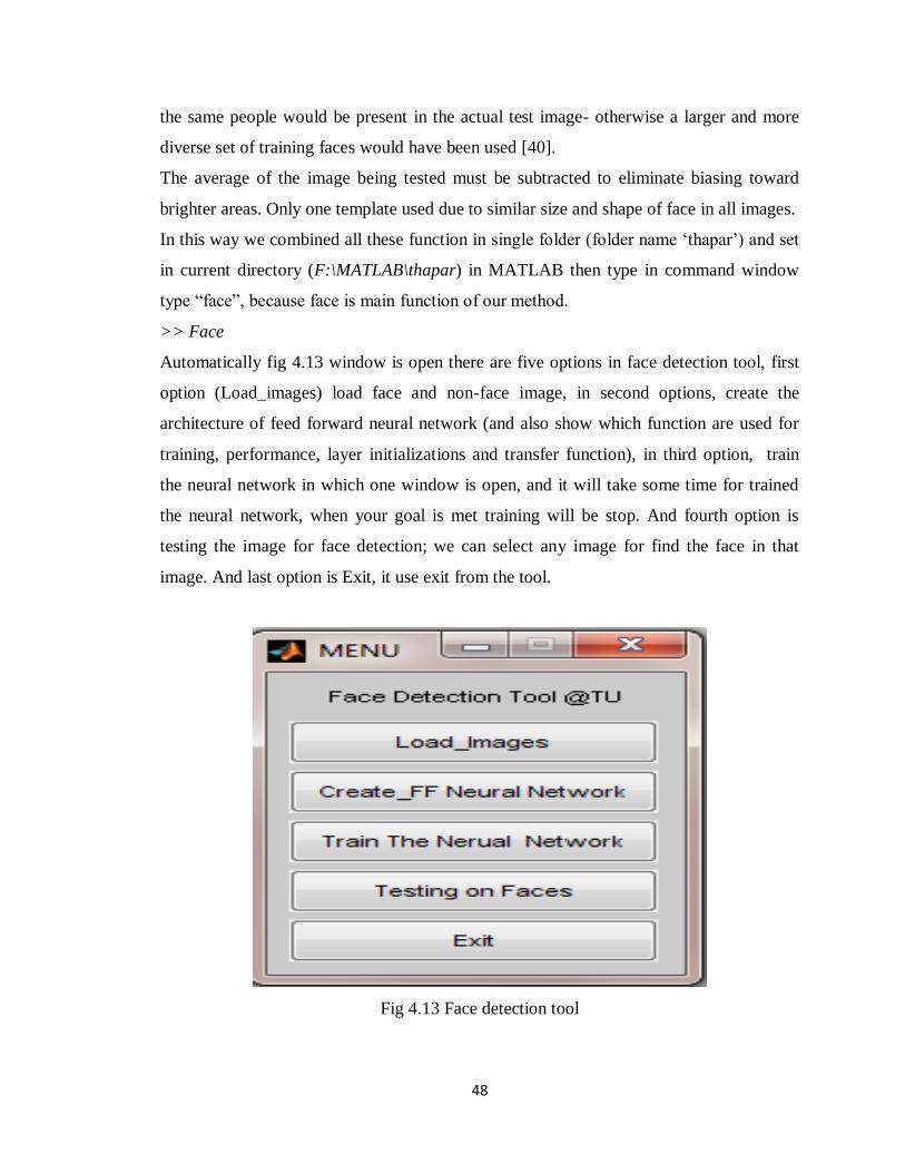
48
the same people would be present in the actual test image- otherwise a larger and more
diverse set of training faces would have been used [40].
The average of the image being tested must be subtracted to eliminate biasing toward
brighter areas. Only one template used due to similar size and shape of face in all images.
In this way we combined all these function in single folder (folder name „thapar‟) and set
in current directory (F:\MATLAB\thapar) in MATLAB then type in command window
type “face”, because face is main function of our method.
>> Face
Automatically fig 4.13 window is open there are five options in face detection tool, first
option (Load_images) load face and non-face image, in second options, create the
architecture of feed forward neural network (and also show which function are used for
training, performance, layer initializations and transfer function), in third option, train
the neural network in which one window is open, and it will take some time for trained
the neural network, when your goal is met training will be stop. And fourth option is
testing the image for face detection; we can select any image for find the face in that
image. And last option is Exit, it use exit from the tool.
Fig 4.13 Face detection tool

49
Chapter 5
Result and Testing
Four different network parameters were chosen based on the transformation and training
function. All the four-network scenarios are listed below in table 5.1. In this chapter we
will discuss the performance of each network one by one and in the end a comparative
study of these four networks is presented.
Table 5.1 Network combinations
Transformation/training
function
FFT DCT
TRAINSCG FFT_TRAINSCG DCT_TRAINSCG
TRAINCGB FFT_TRAINCGB DCT_TRAINCGB
5.1 Result of FFT_TRAINSCG
In this section we are using Fast Fourier transform and training function trainscg for train
the neural network.
.
Fig 5.1 Training with TRAINSCG

50
Fig 5.1 shows the training of network FFT_TRAINSCG. The performance goal was met
in 145 epochs.
Fig-5.2 Snapshot of training performance (TRAINSCG)
After meeting the goal the system was tested with test pattern/images. In the training set
some false images was also tested. The image was image of animal face. This was done to
test if the network recognizes focus in general (i.e. two eyes, a nose and a mouth), or
something unique about human face. These animal faces were not the part of the training
set provided for training the system. The network detected this dog‟s face. The region
after all does have two eyes; the skin of the dog is dark in the middle, which makes it
appear somewhat like a nose.
In table 5.2 show the data of 7 images including size, Num of Faces, Num of Hit, Num of
Repeat, Num of False, and Num of miss face in given image. The False_postive rate and
False negative rate which depends upon the number of missed false face and number of
incorrectly detected face respectively.

51
Fig-5.3 Testing of image(FFT_TRAINSCG)
Table 5.2 below shows the results for FFT_TRAINSCG. The accuracy is obtained by using the
following equation [3].
Accuracy (in %) =100-(false positive rate+ false negative rate) ………… (3)
Table5.2 Face Detection Results using 7 Test Images with FFT_TRAINSCG S
ize_of_
imag
e
Num
_ F
aces
Num
_H
it
Num
_ R
epeat
Num
_F
alse
Num
_m
iss
run tim
e [sec]
False_
postiv
e
(%)
False
neg
ative(%
)
Accu
racy
Dog1.jpg 60X59 1 1 0 0 0 8.674004 00 00 100
Mon2.jpg 128X93 1 1 0 0 0 0.994095 00 00 100
3.jpg 150X150 7 6 0 1 1 58.51247 14.28 14.28 71.27
4.jpg 150X65 7 7 0 0 0 23.413958 00 00 100
5.jpg 130X96 15 14 0 1 1 51.352306 6.66 6.66 86.66
6.jpg 226X108 4 3 1 1 1 16.706838 25 25 50.0
Im4.jpg 600X254 60 56 9 14 4 894.24289 6.66 23.33 70.1

52
Num_ Faces: total number of faces in the picture
Num_ Hit: number of faces successfully detected
Num _ Repeat: number of faces repeatedly detected
Num_ False: number of case where a non-face is reported
Num_miss: number of missed face (Num_faces-Num_hit)
run time : run time of the face detection routine
* run time measure in C2D processor, 2.66 MHz, 2.00 GB RAM
The face detection algorithm (FFT_TRAINSCG) shows 92.006 % of average right hit
rate, 5.714 % of average repeat rate, 9.89 % of average false hit rate and average
accuracy is 82.56% for 7 training images. The average false positive rate and false
negative rate are 11.19 % and 5.17 % respectively. The average run time is 287.4026
seconds.
5.2 Result of DCT_TRAINSCG
In this section we are using discrete cosine transform (DCT) and training function
trainscg for train the neural network.
Fig 5.4 Snapshot of training performance with DCT_TRAINSCG

53
Fig 5.5 shows the training of network DCT_TRAINSCG. The performance goal was met
in 117 epochs.
Fig-5.5 Training with TRAINSCG
Testing of images is shown in Fig 5.6 using DCT_TRAINSCG.
Fig-5.6 Testing of image with DCT_TRAINSCG
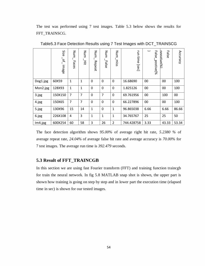
54
The test was performed using 7 test images. Table 5.3 below shows the results for
FFT_TRAINSCG.
Table5.3 Face Detection Results using 7 Test Images with DCT_TRAINSCG
Size _of_ im
age
Nu
m_ Faces
Nu
m _H
it
Nu
m_ R
epeat
Nu
m _False
Nu
m_m
iss
run
time [sec]
False_p
ostive(%
) False
negative(%
)
Accu
racy
Dog1.jpg 60X59 1 1 0 0 0 16.68690 00 00 100
Mon2.jpg 128X93 1 1 0 0 0 1.825126 00 00 100
3.jpg 150X150 7 7 0 7 0 69.761956 00 100 00
4.jpg 150X65 7 7 0 0 0 66.227896 00 00 100
5.jpg 130X96 15 14 1 0 1 96.865038 6.66 6.66 86.66
6.jpg 226X108 4 3 1 1 1 34.765767 25 25 50
Im4.jpg 600X254 60 58 3 26 2 744.428758 3.33 43.33 53.34
The face detection algorithm shows 95.00% of average right hit rate, 5.2380 % of
average repeat rate, 24.04% of average false hit rate and average accuracy is 70.00% for
7 test images. The average run time is 392.479 seconds.
5.3 Result of FFT_TRAINCGB
In this section we are using fast Fourier transform (FFT) and training function traincgb
for train the neural network. In fig 5.8 MATLAB snap shot is shown, the upper part is
shown how training is going on step by step and in lower part the execution time (elapsed
time in sec) is shown for our tested images.

55
Fig-5.7 Training with TRAINCGB
Fig-5.8 Snapshot of training performance with FFT_TRAINCGB
Fig 5.7 shows the training of network FFT_TRAINCGB. The performance goal was met
in 51 epochs.
Testing of images is shown in Fig 5.9 using FFT_TRAINCGB.

56
Fig-5.9 Testing of image(FFT_TRAINCGB)
The test was performed using 7 test images. Table 5.4 below shows the results for
FFT_TRAINCGB.
Table5.4. Face Detection Results using 7 Test Images FFT_TRAINCGB
Size _
of_
imag
e
Nu
m_
Faces
Nu
m _
Hit
Nu
m_
Rep
eat
Nu
m _
False
Nu
m_
miss
run
time [sec]
False_
po
stive
(%)
False n
egativ
e
(%)
Accu
racy
Dog1.jpg 60X59 1 1 0 0 0 4.983142 0 0 100
Mon2.jpg 128X93 1 1 0 0 0 1.585485 0 0 100
3.jpg 150X150 7 7 1 0 0 76.121917 0 0 100
4.jpg 150X65 7 7 0 0 0 47.652360 0 0 100
5.jpg 130X96 15 13 0 1 2 138.089432 6.666 13.333 80.0
6.jpg 226X108 4 3 0 2 1 19.477857 50.00 25.00 25
Im4.jpg 600X254 60 59 7 13 1 900.66254 21.6666 1.66 78.31

57
The face detection algorithm shows 94.28% of average right hit rate, and 3.707% of
average repeat rate, and 11.190 % of average false hit rate for 7 test images. The average
Accuracy is 83.33%. The average run time is 416.576 seconds.
5.4 Result of DCT_TRAINCGB
In this section we are using discrete cosine transform (DCT) and training function
traincgb for train the neural network.
Fig-5.10 Training withTRAINCGB
Fig-5.11 Snapshot of training performance of DCT_TRAINCGB

58
Fig 5.11 show how our performance goal met it start from 0 epochs and performance is
1.60692 but after some time epochs is 54 (as shown in fig 5.10), the performance is
0.000957358 and performance goal met.
Testing of images is shown in Fig 5.12 using DCT_TRAINCGB, and results are different
from other training method.
Fig-5.12 Testing of image(DCT_TRAINCGB)
The test was performed using 7 test images. And also calculate the false positive rate,
false negative rate, and accuracy of the method. In fig 5.11 MATLAB snap shot is
shown, the upper part is shown how training is going on step by step and in lower part the
execution time (elapsed time in sec) is shown for our tested images. Table 5.5 below
shows the results for DCT_TRAINCGB.

59
Table 5.5 Face Detection Results using 7 Test Images with DCT_TRAINCGB
The face detection algorithm shows 96.428 % of average right hit rate, 0.952% of
average repeat rate, and 43.945% of average false hit rate for 7 test images. The average
Accuracy is 52.481%. The average run time is 730.270 seconds.
5.5 Comparison of result
Table 5.6 describe the comparisons of four techniques in term of Average accuracy, right
hit rate, repeat rate, false hit rate and run average time. This is also depicted in the form
of graph shown in below.
Table 5.6 Result comparison
FFT_TRAINSCG DCT_TRAINSCG FFT_TRAINCGB DCT_TRAINCGB
AVERAGE_ACCURACY 82.56 70.00 83.33 52.481
RIGHT_HIT_RATE 92.006 95.00 94.285 96.428
REPEAT_RATE 5.714 5.2380 3.707 0.952
FALSE_HIT_RATE 9.89 24.04 11.190 43.945
RUN_AVERAGE_TIME(in
sec)
287.4026 392.479 416.576 730.270

60
5.6 Performance Analysis
A graph has been drawn from table 5.6 for comparing the performance statistics in term
of average accuracy, right hit rate, repeat rate and false hit rate. In y-axis measurement is
in percentage (%) and in x-axis four algorithms are given with four measurements
0102030405060708090
100
Per
form
ance
(in
%)
Algorithms Parameters
Performance Analysis of Four Combination
AVERAGE_ACCURACY
RIGHT_HIT_RATE
REPEAT_RATE
FALSE_HIT_RATE
Fig 5.13 a graph comparing the performance statistics

61
Chapter 6
Conclusion and Future scope
6.1 Conclusion
We presented a neural network based face detection system. Our experiments have
shown that using MLP neural networks for face detection is a very promising approach.
The model‟s robustness has been obtained with a back propagation learning algorithms
and the tansig () activation function. Sets of seven training images were used for this
purpose. The objective was to design and implement a face detector in MATLAB that
will detect human faces in an image similar to the training images.
In the MATLAB we compared the results with 7 images taking four combinations
(FFT_TRAINSCG, DCT_TRAINSCG, FFT_TRAINCGB and DCT_TRAINCGB). The
four-face detection algorithm combinations shows average accuracy is 82.56%, 72%,
83.33% and 52.481% respectively. In our approach no preprocessing is needed since the
normalization is incorporated directly in the weights of the input network.
6.2 Future scope
The future work can be extended to build a system, which can deal with larger rotations it
seems necessary to train a set of classifiers on a database of rotated faces, with each
classifier being tuned to a specific range of rotations. A system for face detection must be
developed, which can give more accurate results in term of right hit rate, repeat rate, false
hit rate, average accuracy and average run time. The performance statistics shows an
improvement in the detection rate, but an accompanying increase in the number of false
positives. The goal of any future improvement should be to improve the detection rate,
minimize the number of false positives, and improve the speed of the detection process.
A good place to start would be to aim to minimize the number of false positives.
62
Reference
[1] S. N. Sivanandam, S. Sumathi, and S. N. Deepa, “Introduction to Neural
Networks using MATLAB 6.0”, vol. 1, Tata McGraw-Hill 2006.
[2] Aamer, S.S.Mohamed, Ying Weng, Stan S Ipson, and Jianmin Jiang, “Face
Detection based on Skin Color in Image by Neural Networks”, School of
Informatics, University of Bradford, IEEE SSD'08, July 2008.
[3] Z. Sadri Tabatabaie, R.W.Rahmat, N. I. Udzir and E. Kheirkhah, “A Hybrid Face
Detection System using combination of Appearance-based and Feature-based
methods”, IJCSNS International Journal of Computer Science and Network
Security, vol.9 no.5, May 2009.
[4] Biological Neuron, URL: http://faculty.washington.edu/chudler/color/pic1an.gif,
June 2010.
[5] Neural Networks, URL: http://www.doc.ic.ac.uk/~nd/surprise_96/journal/
vol4/cs11/report.html, June 2010.
[6] Hassoun, M.H., “Fundamentals of Artificial Neural Network”, Fourth Edition
MIT press, 1995.
[7] The Math Work, the neural network and image processing toolbox, The Math
Work Inc. 1999.
[8] C. S. Rapp and W. L. Joyner, "Image Processing and Image Enhancement",
Johnson City, Texas, 1996.
[9] Artificial Neuron, URL: http://research.yale.edu/ysm/images/78.2/articles-neural-
neuron.jpg, June 2010.
[10] R. Bala, K.M.Braun, "Color-to-Grayscale Conversion to Maintain
Discriminability", Xerox Innovation Group, 800 Phillips Rd, 128-27E, Webster,
NY 14580, 2004.
[11] M. Qiu, G. D. Finlayson, G. Qiu, "Contrast Maximizing and Brightness
Preserving Color to Grayscale Image Conversion", CGIV2008, 4th European
Conference on Color in Graphics, Imaging, and Vision, June 9 – 13 2008.
[12] William, K. Pratt, “Digital Image Processing”, Fourth Edition, A John Wiley &
Sons Inc. Publication, pp.465-529, 2007.

63
[13] M.J.D. Powell, “Restart procedures for the conjugate gradient method”,
Mathematical Programming, Vol. 12, pp. 241-254, 1977.
[14] V. Cherkassky, F. Mulier, “Learning from data; Concepts, Theory, and
Methods" 1st edition, John Wiley & Sons, Inc. New York, 1998.
[15] I. Craw, D. Tock, and A. Bennett, “Finding face features”, Proc. of 2nd
European Conf. Computer Vision. pp. 92-96, 1992.
[16] N. Huijsmans and M. S. Lew, “Information Theory and Face Detection”, proc
Int1 Conf. Pattern Recognition, pp.601-605, Aug 1996.
[17] R.Cipolla and K.C.Yow, “Feature Based Human Face Detection”, Image
Processing and vision Computing, vol.15, no.9, pp.713-735, sept.1997.
[18] T.S.Huang and A.J.Colmenarez “Face detection with Information Based and
Maximum Discrimination”, IEEE Int1 Conf. Computer Vision and Pattern
Recognition, pp.782-787, 1997.
[19] T. Poggio and K. K. Sung, “Example Based Learning for View Based Human
Face Detection”, IEEE Trans. Pattern Analysis and Machine Intelligence,
vol.20, no.1, pp.39-51, Jan.1998.
[20] N. Ahuja and M.H. yang, “Detecting Human Face in color image”, Proc IEEE
Int 1, Conf. Image Processing, pp.127-139, Oct 1998.
[21] S. Baluja, H. A. Rowley and T. Kanade, “Neural Network Based Face
Detection”, IEEE trans. Pattern Analysis and Machine Intelligence, vol.20, no.1,
pp.23-38, Jan 1998.
[22] S. Baluja, H. A. Rowley and T. Kanade, “Rotation Invariant Neural network
Based Face dictation”, proc IEEE conf. Computer Vision and Pattern
Recognition, pp.38-44, 1998.
[23] G. Garcia and G. Tziritas, “Face Detection Using Quantized Skin Color
Regions Merging and Wavelets Packet Analysis”, trans. Multimedia vol.1, no.3,
pp. 264-277, Sept.1999.
[24] Q. Chen, H.WU and M.Yachida, “Face detection from color Images Using A
fuzzy Pattern Matching intelligence”, vol. 21, no.6, pp.557-563, June1999.
[25] D. Maio and D. Maltoni, “Real time Face Location on Gray Scale Static
Images”, Pattern Recognition, vol.33, no.9, pp.1525-1539, Sept 2000.

64
[26] R. Feraud, O. j. Bernier, J. E. Viallet and M. Collobert, “A Fast and Accurate
Face Detection Based on Neural Network”, IEEE transition, Pattern Analysis
and Machine Intelligence, vol. 23, no.1, pp.42-53, Jan 2001.
[27] R.L. Hsu, M. A. Mottaleb and A. K. Jain, “Face Detection in Color Images”,
IEEE transactions on Pattern Analysis and Machine Intelligence, vol. 24, no. 5,
May 2002.
[28] R. C. Verma, C. Schmid, and K. Mikolajczyk, “Face Detection and Tracking in
a Video by Propagating Detection Probabilities”, IEEE transaction on pattern
analysis and machine intelligence, vol.25, no. 10, October 2003.
[29] S. W. Christian Igely and U. Handmann, “Evolutionary Optimization of Neural
Networks for Face Detection”, European Symposium on Artificial Neural
Networks (ESANN) 2004.
[30] Y. Chen, S. Jiang and A. Abraham, “Face Recognition Using DCT and Hybrid
Flexible Neural Tree”, doi.7803-9422-4/05, pp.1459-1463, 2005.
[31] Uma D. Nadimpalli, Randy R. Price, Steven G. Hall, and Pallavi Bomma, “A
Comparison of Image Processing Techniques for Bird Recognition”, Biotechnol.
Prog. Vol. 2, pp. 9-13, 2006.
[32] J. Choi, Y.S. Chung, K.H. Kim and J. H. Yoo, “Face Recognition Using Energy
Probabllity In DCT Domain”, ICME 2006, pp.1549-1552, 2006.
[33] Abdallah S. Abdallah, A. Lynn Abbott, and Mohamad Abou El-Nasr, “A New
Face Detection Technique using 2D DCT and Self Organizing Feature Map”,
World Academy of Science, Engineering and technology ISSUE 27, 2007.
[34] W. Zhanjie and T. Li, “Face Detection Based on skin Color and Neural
Network”, International Conference on Computer Science and Software
Engineering, pp. 961-964, 2008.
[35] A. Lanitis, C. J. Taylor, and T. F. Cootes, “An automatic face identification
system using flexible appearance models”, Image and Vision Computing,
vol.13, no.5, pp.393-401, 1995.
[36] D. Lyon and N. Vincent, “Interactive Embedded Face recognition” Journal of
object technology vol. 8, no. 1, January-February 2009.

65
[37] Hazem M. El. Bakry and Qiangfu Zhao, “Fast Object/Face Detection Using
Neural Networks and Fast Fourier Transform”, International Journal of Signal
Processing 1; 4 pp.182-187, 2005.
[38] J. Zeb, M. Y. Javed, and U. Qayyum, “Low Resolution Single Neural Network
Based Face Recognition”, World Academy of Science, Engineering and
Technology ISSUE 28, 2007.
[39] E. Sackinger, B.E. Boser, J. Bromley, Y. Lecun, and L. D. jacket, “Application
of the ANNA neural network chip to high speed character recognition”, IEEE
transaction on neural networks, vol.3.3 pp. 498-505, 1992.
[40] J. Wang and H. Yang, "Face Detection Based on Template Matching and
2DPCA Algorithm", CISP'08 Congress on Image and Signal Processing, Sanya,
Hainan, China, pp. 575-579, 2008.
[41] MATLAB and Simulink for Technical Computing, URL:
http://www.mathworks.com, June 2010.
[42] B. Yegnanarayana, “Artificial Neural Networks”, Eight Printing, Prentice-Hall
of India Limited, pp. 306-322, August 2003.

66
List of Paper Published/Communicated
1. Tarun Kumar, Kushal Veer Singh and Karun Verma, “Artificial Neural Network
in Image Recognition”, Presented at 2nd
national Seminar on Recent Trends in
Advanced of Mathematical and Physical Science (RTAMPS-2010), Meerut, India
Jan 30-31, 2010.
2. Tarun Kumar, Kushal Veer Singh and Karun Verma, "Preprocessing Stage for
Image Recognition using MATLAB”, published at National Conference on Next
Generation Computing (NGC-10), GITM Gurgaon, India, 20 March 2010.
3. Tarun Kumar, Kushal Veer Singh and Karun Verma, "Artifical Neural Network in
Face Detection", communicated at 1st International Conference on Parallel,
Distributed and Grid Computing (PDGC-2010), JUIT Waknaghat, Solan (HP),
India, October 28 to 30, 2010.
4. Tarun Kumar and Karun Verma, "A Theory for Conversion RGB to Gray image”,
communicated at International Conference On Computer and Communication
Technology (ICCCT 2010), MNIT Allahabad, India, September 17-19, 2010.
5. Tarun Kumar and Karun Verma, "Soft Computing Techniques Comparison for
Face Detection", communicated at PRAGYAAN: Journal of Information
Technology, IMS Dehradun, India.