Embed Size (px)
Citation preview

Masteruppsats i matematisk statistikMaster Thesis in Mathematical Statistics
Analysis of stochastic claimsreserving uncertaintyNicole Li

Matematiska institutionen
Masteruppsats 2017:4FörsäkringsmatematikMaj 2017
www.math.su.se
Matematisk statistikMatematiska institutionenStockholms universitet106 91 Stockholm
Mathematical StatisticsStockholm UniversityMaster Thesis 2017:4
http://www.math.su.se
Analysis of stochastic claims reserving
uncertainty
Nicole Li∗
May 2017
Abstract
Traditionally, the claims reserves are settled by using determin-
istic methods such as chain-ladder method. However, the question
of statistical quality of the reserve estimates can not be answered
unless a model is found. The goal of this thesis is to analyze the un-
certainty of the reserve which comes from a stochastic model called
Over-dispersed Poisson model. To achieve the purpose, a data-set of
one product for the past 24 years’ period is used. The analysis is done
by checking the underlying assumptions of the stochastic reserving
model, testing different distributions and investigating the ultimate
risk and the one-year reserve risk by three simulation methods. Based
on the real data and the results of the back test, we can conclude that
the Over-dispersed Poisson model works well. The results in all three
risk analyses indicate that the Over-dispersed Poisson model works as
expected when the underlying assumptions are fulfilled.
∗Postal address: Mathematical Statistics, Stockholm University, SE-106 91, Sweden.
E-mail: [email protected]. Supervisor: Mathias Lindholm.

Contents
1 Introduction 1
1.1 Problem statement and Purpose . . . . . . . . . . . . . . . . . 1
1.2 Structure of the thesis . . . . . . . . . . . . . . . . . . . . . . 2
1.3 Data material . . . . . . . . . . . . . . . . . . . . . . . . . . . 2
2 Theory 3
2.1 Terminology . . . . . . . . . . . . . . . . . . . . . . . . . . . . 3
2.2 Error types . . . . . . . . . . . . . . . . . . . . . . . . . . . . 3
2.3 Chain Ladder algorithm . . . . . . . . . . . . . . . . . . . . . 4
2.4 Negative incremental claims . . . . . . . . . . . . . . . . . . . 6
2.5 Claims development result . . . . . . . . . . . . . . . . . . . . 6
3 Methodology 7
3.1 Stochastic models associated with the CL algorithm . . . . . . 7
3.1.1 Mack’s distribution-free chain-ladder model . . . . . . 7
3.1.2 Poisson and over-dispersed Poisson model . . . . . . . 9
3.2 Predictive distribution of claims reserve . . . . . . . . . . . . . 13
3.3 Best Estimate . . . . . . . . . . . . . . . . . . . . . . . . . . . 13
3.4 Ultimate risk . . . . . . . . . . . . . . . . . . . . . . . . . . . 13
3.5 One-year-reserve risk . . . . . . . . . . . . . . . . . . . . . . . 14
3.6 Simulation . . . . . . . . . . . . . . . . . . . . . . . . . . . . . 15
3.6.1 Method 1 . . . . . . . . . . . . . . . . . . . . . . . . . 15
3.6.2 Method 2 . . . . . . . . . . . . . . . . . . . . . . . . . 16
3.6.3 Method 3 . . . . . . . . . . . . . . . . . . . . . . . . . 17
4 Analysis & Findings 18
5 Discussion and Conclusion 26
6 Limitations and future researches 28
7 References 29
8 Appendix 30
ii

1 Introduction
Insurance industries can be classified into two categories: life insurance and
non-life insurance. There are different characteristics between life and non-
life insurance products, such as terms of contracts, type of claims, risk drivers,
etc. A typical non-life insurance claim can be illustrated in a process as in
which an accident occurred at a time in the insurance period and then re-
ported some time later at the reporting date and finally the claim being
settled at a further later time point by closing date. For certain cases, due to
certain reasons, for example, new evidence is discovered for a settled claim,
it leads that the closed claim has to be reopened (Huang & Wu, 2012).
Claims reserve is money that is earmarked for the eventual claim payment.
It is a future obligation of an insurance company. For the purpose of val-
uation and financial reporting, the insurers predict the ultimate payment
amount for all the claims. This includes estimates of both Incurred But Not
Reported (IBNR) and Reported But Not Settled (RBNS) claims. It is es-
sential to understand the importance of setting the right claim cost since the
reserve is classified as a liability in the company balance sheet and a reserve
which is wrongly estimated can represent a false picture of the company’s
financial state to shareholder and investors. If the reserve is underestimated
the insurance company will not be able to fulfil its undertakings and if it is
overestimated the insurance company unnecessarily holds the excess capital
instead of using it for other purposes, e.g. for investments with potentially
higher return.
1.1 Problem statement and Purpose
Traditionally, the claims reserves are estimated by using deterministic meth-
ods. The chain-ladder method can be considered as the most famous deter-
ministic method which is described as a mechanical algorithm rather than a
full statistical model. The biggest advantage of this approach is its simplicity
and transparency even for non-actuaries who are involved in the reserving
process. However, the question of statistical quality of the reserve estimates
can not be answered unless a statistical model is found underlying the algo-
1

rithm.
Within the stochastic claims reserving area, many models have been dis-
cussed and applied widely in the academic literature. Each model requires
different assumptions. Generalized linear model and bootstrapping of deter-
ministic model are popular techniques in common use. The purpose of this
thesis is to analyze the uncertainty of the estimated reserves which come
from a stochastic model called Over-dispersed Poisson model for a Swedish
insurance company. Moreover, the study aims to analyze the underlying
assumptions of this stochastic model based on given data and also to investi-
gate the ultimate risk and the one-year reserve risk where the risk estimation
follows naturally from the stochastic model constructions.
1.2 Structure of the thesis
A literature review is conducted together with a presentation of the theory
is given in section 2. The methodologies used in this thesis are introduced
in section 3. In section 4, the empirical analysis and results are presented.
Discussion and conclusion are summarized in section 5. Finally, limitations
and future researches will be found in the last section.
1.3 Data material
The data used in this study is taken from a Swedish insurance company. It
contains the real payments, the amount of reserves for RBNS-claims and the
number of reported claims for one product for the past 24 years disposed
in the traditional way according to accident year and development period.
For the reason of confidentiality, the data has been distorted by multiplying
all the values with the same constant. There are around 1,867,187 events in
the data set excluding zero claims. In extensions to these claims we also use
information from around 196,777 zero claims. Zero claims are those claims
that contain neither payments nor outstanding reserves.
2

2 Theory
2.1 Terminology
This section introduces some basic terminologies used within insurance in-
dustry.
There are two types of outstanding claims which need to be estimated for
claims reserving, RBNS (Reported But Not Settled) and IBNR (Incurred But
Not Repported). RBNS is the claim that insurance has been aware of. The
payment has started but the full payment has not been carried out yet. The
calculation of RBNS takes consideration of the payment pattern according
to the insurance company. It also requires an understanding of where claims
are in the settlement process. IBNR is the event that the actual losses have
been incurred, but have not officially been reported. Actuaries will estimate
the potential damages to the event. Based on the actuaries’ estimations the
insurance company may decide to set up reserves to allocate liquid assets to
those expected losses.
Ultimate loss is the total sum of insurer’s payments for a fully developed
loss to the insured (i.e. paid losses plus outstanding reported losses (RBNS)
and incurred but not reported (IBNR) losses). In order to estimate the IBNR
claims, actuaries usually start with estimating the ultimate loss using differ-
ent algorithms for example Chain-Ladder or Bornhuetter-Ferguson. From
the estimated ultimate loss, the IBNR can be determined.
The term ”claims reserve” refers to the expected value of the future pay-
ments from RBNS and IBNR i.e. Rtot = RRBNS +RIBNR.
2.2 Error types
The following describes different types of the uncertainty characteristics of
the outstanding claims liabilities. These uncertainties can be divided into
three categories (Daykin, Pentikainen, & Pesosnen, 1994).
3
Parameter error – Due to the sampling variation of the past claims data
and the limited quantity of observations, the exact values of parameters are
unknown. Thus, the uncertainty of parameter estimation exists.
Process error (or stochastic error) – Due to the random fluctuations of the
exact amounts of the future payments even in the situation that parameters
and model are correct, the process error exists.
Model error – Due to the fact that the model adopted are uncertain and
only approximations to the underlying claims development mechanism.
This paper focuses on measuring the parameter error, even called estima-
tion variance, and the process error. The model error will be considered by
testing different model assumptions when applying the reserving model to
the same set of claims data. The sum of the process variance and the estima-
tion variance is called prediction variance and is a measure of the variability
of the prediction. The mean squared error of the prediction (MSEP) is used
for prediction variance and is defined by England and Verrall (2002) as
MSEPi = E[(Ri − Ri)2] = V ar(Ri) + V ar(Ri) (1)
where Ri is the estimator of Ri.
In addition, V ar(Ri) allows for the process error and V ar(Ri) allows for
the parameter error.
2.3 Chain Ladder algorithm
This part is supposed to give a short description of the chain-ladder algo-
rithm which is presented by Mack (1993a). The classical reserving method
is based on the triangle of the aggregate data. Let i denote the year that
accident occurs, i.e. the accident year and j denote the development year.
The data is aggregate by accident year and development year. An example
of run-off triangle on the aggregate data is
4

Known Future payments
C1,1 C1,2 C1,3 C1,4
C2,1 C2,2 C2,3 C2,4
C3,1 C3,2 C3,3 C3,4
C4,1 C4,2 C4,3 C4,4
where Ci,j denotes the total cumulative claims amount from accident year i
until development year j. The claims in the north-western triangle are known
values.
The idea of the chain-ladder algorithm is that all accident years have the
similar behaviours and the cumulative claims amounts are approximately
the claims amounts at the last development year multiplying a factor i.e
Ci,j+1 = fjCi,j (2)
The factor fj is called chain-ladder (CL) factors, age-to-age factors or link
ratios and is calculated as
fj =
∑I−j−1i=1 Ci,j+1∑I−j−1i=1 Ci,j
(3)
With CL factors we predict the ultimate claim Ci,J for i + J > I at time
t = I by
Ci,J = Ci,I−i
J−1∏j=I−i
fj (4)
Thus, the reserve at time t = I for accident year i > I − J is
Ri = Ci,J − Ci,I−i (5)
By aggregating over all accident years the outstanding loss liability of the
past exposure claims is
R =J∑
i=I−J+1
Ri (6)
5

2.4 Negative incremental claims
Sometimes there exists negative values in the development triangle of in-
cremental claim amounts. Typically they are consequences of the already
reported claims which are cancelled due to the initial overestimation of the
loss or the insurance company receives payments from third parties (Gould,
2008). Some methods of claims reserving may produce reserve estimates even
there exists negative values. However, for some methods, the results would
be unreliable when the negative increment values involves.
There has been suggested different solutions on how to handle the nega-
tive incremental claims. One method involves adding one positive constant
on all increment claims. The constant needs to be subtracted after the anal-
ysis is completed. This method provides suitable results as long as there
are not too many negative claims (Gould, 2008). However, this procedure
makes the variability of the result depend on the constant added earlier.
Another method to adjust the negative payments is to cancel matching pos-
itive amounts if there exists. If no matching positive amounts exist then the
amount is subtracted from previous payments.
2.5 Claims development result
Wuthrich, Merz & Lysenko (2007) and Wuthrich (2015) give a definition of
the claims development result.
CDRi,t+1 = Rti − (X t+1
i +Rt+1i ) = Ct
i,J − Ct+1i,J . (7)
where Rti is the best estimate reserves at time t ≥ I for accident year i > t−J .
Ctj,J is the ultimate claim of accident year i at time t ≥ I. Xi,t−i+1 is the
payment between t and t+ 1.
If the claims development result is positive we have a gain because we have
overestimated the outstanding loss liabilities at time t, otherwise we have a
loss.
The uncertainty in this position measured by MSEP with given information
6

D:
MSEPCDRi,t+1|D = E[(CDRi,t+1 − CDRi,t+1)2|D] (8)
3 Methodology
3.1 Stochastic models associated with the CL algo-
rithm
The most weakness of the chain-ladder method is that it is a deterministic al-
gorithm hence the uncertainty of the reserve estimate can not be determined.
To amend this shortcoming, the stochastic models associated with the chain-
ladder algorithm have been developed. The variation of the estimate from
the models is possible to be analyzed. In this section, the stochastic models
underlying the chain-ladder algorithm will be presented as well as the under-
lying assumptions for each model. In this section we also aim to show that
these stochastic models indeed provide the same estimates as the chain-ladder
method.
3.1.1 Mack’s distribution-free chain-ladder model
Thomas Mack (1993a) proposed a distribution free stochastic model which
is probably the most common stochastic reserving method. The model pro-
duces equivalent results to the chain-ladder algorithm. Recall, Ci,j represents
the total claims amount. The basic assumptions underlying the stochastic
Mack method are the same as the ones for the deterministic chain-ladder.
Model Assumptions:
CL1 :
There exists development factors f1, ..., fI−1 > 0 so that
E[Ci,j+1 | Ci,1, ..., Ci,j] = fjCi,j (9)
where I is the total development year and the CL factor E[fj] = fj is cal-
culated by formula (3) above. The CL factor fj is the same for all accident
years within development year j.
7

CL2:
{Ci,1, ..., Ci,I}, {Ck,1, ..., Ck,I}, i 6= k, are independent. (10)
CL3:
There exists αj > 0 so that
V ar(Ci,j+1|Ci,1, ..., Ci,j) = Ci,jα2j (11)
where
α2j =
1
I − j − 1
I−j∑i
Ci,j
(Ci,j+1
Ci,j− fj
)2
1 ≤ j ≤ I − 2 (12)
is an unbiased estimator of α2j , 1 ≤ j ≤ I − 2. For estimating α2
I−1 Mack
suggests
α2I−1 = min(α4
I−2/α2I−3,min(α2
I−3, α2I−2)). (13)
As with equation (5) the reserve is given by
Ri = Ci,I − Ci,I+1−i, (14)
Further, Mack (1993a) defines the mean squared error of the estimator Ci,I
of Ci,I by mse(Ci,I), note that this differs from MSEP from equation (1),
which is defined to be
mse(Ri) = mse(Ci,I) = E[(Ci,I − Ci,I)2|D]
= V ar(Ci,I |D) + (E[Ci,I |D)− Ci,I)2(15)
where D = {Cik|i+ k ≤ I + 1}, i.e the set of data observed so far. The first
term V ar(Ci,I |D) represents the process risk and the second term (E[Ci,I |D)−Ci,I)
2 represents the parameter risk.
Formulas used to check the chain-ladder Assumptions
Spearman’s rank correlation coefficient
Let rik, 1 ≤ i ≤ I − k, denote the rank of Ci,k+1/Cik obtained in this
8

way, 1 ≤ rik ≤ I − k. Then doing the same with the preceding develop-
ment factors Cik/Ci,k−1, 1 ≤ i ≤ I − k, leaving out CI−+1−k,k/CI+1−k,k−1 for
which the subsequent development factor has not yet been observed. Let sik,
1 ≤ i ≤ I − k, be the ranks obtained in this way 1 ≤ rik ≤ I − k. Then the
Spearman’s rank correlation coefficient Tk is defined as
Tk = 1− 6I−k∑i=1
(rik − sik)2/((I − k)3 − I + k) (16)
and the (I − k − 1)-weighted average of Tks is defined as
T =I−2∑k=2
(I − k − 1)Tk/I−2∑k=2
(I − k − 1)
=I−2∑k=2
I − k − 1
(I − 2)(I − 3)/2Tk
(17)
3.1.2 Poisson and over-dispersed Poisson model
Renshaw & Verrall (1998) noticed the link between the chain-ladder algo-
rithm and Poisson distribution. They were the first to implement the model
using standard methodology for a full statistical review. The model is in form
of a generalized linear model with a log-link function. Let yi,j denote the in-
cremental claims, remember that the total claims amount Ci,j =∑j
k=1 yi,j.
An example run-off triangle of incremental claims:
y1,1 y1,2 y1,3 y1,4
y2,1 y2,2 y2,3
y3,1 y3,2
y4,1
Model Assumptions:
The Over-dispersed Poisson model assumes that the incremental claims amounts
yi,j are independent Over-dispersed Poisson distributed with mean mij and
variance φmij. The scale parameter φ is unknown and estimated from the
data. The mean can be written with a log-link function.
logmij = µ+ αi + βj (18)
9

where α1=β1=0, i = 1, ..., I connects to the accident years and j = 1, ..., J
connects to the development years.
Further, the model also assumes that the sum of the incremental claims
in column j is non-negative. Note that some negative incremental claims are
allowed. Mathematically,
n−j+1∑i=1
yij ≥ 0 for all j (19)
The estimates of the parameters in the model given in (18) and (19) can
be obtained by MLE (Wuthrich, 2015). The estimates of the aggregate
payments of claims in each accident year i can be obtained from the sums:
Cin = Ci,n−i+1 +n∑
j=n−i+2
eµ+αi+βj(i = 1, 2, ..., n) (20)
where µ, αi and βj are the maximum likelihood estimates of the parameters.
Further, we prove that the generalized linear model with Poisson distribution
gives exactly the same results as the chain-ladder algorithm under assump-
tions.
Let p(i),j denote the probability that a claim with accident year i is reported
in development year j. Then
p(i),j =pj∑n−i+1
k=1 pk(21)
where pj is the probability that a claim is reported in development year j
and∑n
k=1 pk = 1. Note that the right side in equation (21) is independent of
i. This last assumption implies that we assume that all claims are reported
by the end of development year n.
Using the multinomial distribution, the conditional likelihood Lc is given
by
Lc =n∏i=1
(Ci,n−i+1!∏n−i+1j=1 yij!
n−i+1∏j=1
pyij(i)j) (22)
10

and consider the estimate for the accident year which has been reported up
to development year index j, the estimate of ultimate cumulative claims for
accident year n− j + 1 is
Cn−j+1,n =Cn−j+1,j
1−∑n
k=j+1 pk. (23)
This can be compared with the chain-ladder estimates:
Cn−j+1,n = Cn−j+1,jλj+1λj+2...λn (24)
where
λj =
∑n−j+1i=1 Cij∑n−j+1
i=1 Ci,j−1
. (25)
Rosenberg (1990) derived a technique for obtaining the estimates pj which
is recursive.
pj =y1j + y2j + ...+ yn−j+1,j
C1n + C2,n−1
1−pn + ...+Cn−j+1
1−pj+1−...−pn
=y1j + y2j + ...+ yn−j+1.j
C1n + C2,n + ...+ Cn−j+1,n
(26)
Note that pn = yinC1n
.
From equations (23) and (24) it can be seen that
λj+1λj+2...λn =1
1− pj+1 − pj+2 − ...− pn(27)
and
λjλj+1...λn =1
1− pj − pj+1 − ...− pn(28)
Thus
λjλj+1...λn =1
1
λj+1λj+2...λn− pj
(29)
and
λj =1
1− pjλj+1λj+2...λn(30)
11

For j = n and since
λn =1
1− pnfrom (30)
=1
1− y1nC1n
from (26)
=Cin
C1n − y1n
=C1n
C1,n−1
(31)
We rewrite the equation (26) as
pj =y1j + y2j + ...+ yn−j+1,j
C1n + C2,n−1λn + ...+ Cn−j+1,jλj+1...λn(32)
Substituting into equation (30)
λj =1
1− y1j+y2j+...+yn−j+1,j
C1n+C2,n−1λn+...+Cn−j+1,j λj+1...λnλj+1λj+2...λn
(33)
and
Cin + C2,n−1λn + ...+ Cn−j+1,jλj+1...λn = λj+1...λn
n−j+1∑i=1
Cij. (34)
Hence, λj can be rewritten as
λj =
∑n−j+1i=1 Cij∑n−j+1
i=1 Cij − (y1j + y2j + ...+ yn−j+1,j)
=
∑n−j+1i=1 Cij∑n−j+1
i=1 Ci,j−1
(35)
which is the chain-ladder estimate.
England & Verrall (2002) give a formula for MSEP which is
MSEP =∑i,j∈∆
φmij +∑i,j∈∆
m2ijV ar(ηij)
+ 2∑
i1j1∈∆,i2j2∈∆
mi1j1mi2j2Cov(ηi1j1 , ηi2j2).(36)
12

where φ is the dispersion parameter and mij = exp(ηij). Note that φmij
corresponds to the plug-in estimation of the theoretical process variance ac-
cording to the Over-dispersed Poisson model. The rest of expression gives
the estimation error.
3.2 Predictive distribution of claims reserve
In this part we aim to present simulation method for finding the whole pre-
dictive distribution of the reserve. There are two main methods which are
currently used for simulation, bootstrapping and Bayesian methods using
Markov Chain Monte Carlo techniques. In this paper only the bootstrap-
ping method will be adopted.
Bootstrapping is a simple simulation-based approach for obtaining the infor-
mation from a sample of data without any knowledge about the underlying
data. By randomly drawing, with replacement, from observed data, a new
data set which is consistent with the underlying distribution will be created.
Bootstrapping is useful only when the underlying model is correctly fitted
to the data. Bootstrapping is applied to the data which are required to be
independent and identically distributed. In this thesis, we combine boot-
strapping method and claims payments’ distribution since the distribution is
a requirement in our researched model.
3.3 Best Estimate
Best estimate is a term used in insurance companies. When we sum over all
the expected payments from RBNS and IBNR claims we get an estimate of
the corresponding reserves, i.e. RRBNS and RIBNR. The total reserve Rtot is
the sum of RRBNS and RIBNR.
3.4 Ultimate risk
The ultimate risk presents the risk of the ultimate loss, in other words, the
uncertainty of the sum of the paid loss, RBNS loss and IBNR loss. With
the simulation method, we obtain a matrix of claims losses. The true total
13

ultimate reserve R can be determined from the matrix. Further we estimate
the claims reserve R using the stochastic model. The ultimate risk is
Uk = Rk −Rk (37)
where Uk is the outcome in simulation number k, k = 1, ..., B. B is the total
number of simulations.
3.5 One-year-reserve risk
Quantifying uncertainty with ranges of possible values and associated prob-
abilities (i.e., with probability distributions) helps everyone understand the
risks involved. Wuthrich, Merz & Lysenko (2007) and Wuthrich (2015) pub-
lish papers about the one-year reserve risk. They perform an analytic for-
mula for the MSEP of the claims development result, see formula (8). Here
we present the work which is done by Ohlsson and Lauzeningks (2009) with a
general simulation approach. This approach will be adopted in this analysis.
Let X t+1 denote the ultimo cost which consists all payments made during
time t and t + 1 for all accident years, Rt denote the opening reserve at the
time t for all accident years and Rt+1 is the closing reserve estimate at time
t+ 1 for all accident years. Then the technical run-off result is given by
T = Rt −X t+1 −Rt+1 (38)
This is same as the CDR definition given in equation (7).
In the Solvency II directive the solvency capital requirement (SCR) for the
standard formula is based on the metric set as 99,5% Value-at-Risk over a
one-year horizon.
p = Pr[L(T ) ≤ V aR] = 99.5% (39)
This means that the SCR of the reserve is the 99,5% quantile of the loss dis-
tribution L of T , which is defined as L(T ) = T . We use simulation method
to obtain the probability distribution by the following three steps.
Step 1: The opening reserve
14

We start by estimating Rt, here the opening reserve is not considered stochas-
tic.
Step 2: Generating the new year
The next step is to generate the claims paid in the next year for each accident
year i.e. we need to generate a new diagonal in the development triangle from
a payment distribution with estimated parameters. By take the sum along
the new diagonal we get the ultimo cost denoted X t+1.
Step 3: The closing reserve
Estimate the reserve Rt+1 with reserving method at time point t+ 1.
3.6 Simulation
This part describes approaches for simulations related to risk analysis. In
order to test the assumption of payment distribution, we compare Poisson
distribution with negative binomial distribution. Note that we simulate pay-
ments from different distributions but always fit an Over-dispersed Poisson
model.
3.6.1 Method 1
Method 1 is related to the ultimate risk. We need to generate incremental
claims payments. We seek a two dimension matrix, the dimensions corre-
spond to the number of the accident years observed. Thus, our matrix is 10
× 10. We use the parameters in table 1 as the start value in the general-
ized linear model and simulate a payment matrix from Poisson distribution
and negative binomial distribution respectively. The matrix is regarded as
observed, thus the observed total ultimate ”true” reserve Rk in simulation
number k is the sum of the elements in the southeast triangle in the ma-
trix. Further, we pretend that only northwest triangle is known and predict
the southeast triangle with the Over-dispersed Poisson model. By sum up
all payments in the new predicted southwest triangle, we obtain the esti-
mated total claims reserve Rk and the ultimate risk Uk in equation (37) for
simulation number k. Repeat the process B times.
15
3.6.2 Method 2
Method 2 is adopted in order to obtain the one-year reserve risk described
in section 3.5.
Step 1
Here we still seek a 10 × 10 matrix of incremental payments. We still use
the parameters in table 1 to simulate a matrix from Poisson distribution and
negative binomial distribution respectively. By using the northwest triangle
from the matrix we calculate the total claims reserve which is the sum of the
reserves for accident years up to development year 10. This is R0 which is
considered non-stochastic.
Step 2
Pretend that only northwest triangle is known and fit an Over-dispersed
Poisson model. Simulate a new diagonal of payments from different distribu-
tions with the new estimated parameters. Let this correspond to simulation
number i and denote the sum of payments with X1i .
Step 3
Given the northwest triangle and simulated payments for next year, predict
the claims reserves for all accident year up to development year 10 with the
Over-dispersed model. Denote the sum of the all reserves with R1i corre-
sponding to simulation number i.
Step 4
Calculate Ti = R0 − (X1i +R1
i ).
Repeat step 2 to 4 B times and obtain a distribution for T by using the
simulated T1, ..., TB. Moreover, from the simulated matrix in step 1, a true
value of
Ttrue = R0true − (X1
true +R1true) (40)
can be determined.
16

3.6.3 Method 3
In the third method, we still need to estimate R0, X1 and R1. To be different
from method 2, the R0 is not fixed.
Step 1
Simulate a 10 × 10 matrix by using the parameters in table 1 from Poisson
distribution and negative binomial distribution respectively.
Step 2
Using the northwest triangle in the matrix to predict claims reserves for all
accident years up to development year 10. Let this correspond to simulation
number i and denote the sum of the claims reserves with R0i .
Step 3
From the simulated matrix in step 1 calculate the total payment for the next
year and denote it with X1i .
Step 4
Given the northwest triangle and the payments for next year predict the
claims reserves for all accident years up to development year 10. Denote the
sum of all claims reserves with R1i .
Step 5
Calculate Ti = R0i − (X1
i +R1i )
Repeat step 1 to 5 B times and obtain a distribution for T by using simu-
lated T1, ..., TB. In this simulation method, we do not use a stochastic claims
reserving method, but we have simulated data and see how the expected
prediction of reserves behaves.
17
4 Analysis & Findings
The data set used in the analysis is a set of claims data for one product from a
Swedish insurance company. The insurance claims are organized by accident
years and development years. It contains the amount of payment for each
reported claim, the amount of reserves for RBNS-claims and the number of
reported claims for last 10 years. When fitting the stochastic chain-ladder
models, only data containing the amount of payments will be used.
Checking the chain-ladder assumptions
We begin with checking the chain-ladder assumptions against the data fol-
lowing the processes presented by Mack (1993b). Here we use the last 10
years’ not full-developed data. As has been pointed out before, the three
basic implicit chain-ladder assumptions are:
(1) E[Ci,k+1 | Ci1, ..., Cik] = Cikfk
(2) Independence of accident years
(3) V ar(Ci,k+1 | Ci1, ..., Cik) = Cikα2k
First, we look at the assumption (1) and (3) for a fixed k and for i = 1, ....I.
There, Cik, 1 ≤ i ≤ I, are considered as given non-random values and the
equation of assumption (1) can be interpreted as an ordinary regression model
of the type
yi = a+ bxi + εi, (41)
where a and b are the regression coefficients and εi is the error term with
E[εi] = 0. In our special case, we have a=0, b = fk i.e. development fac-
tor, k = 1, ..., 8. Further, we have observations of the independent variable
yi = Ci,k+1 at the points xi = Cik for i = 1, ..., I − k. Therefore, we can
estimate the regression coefficient b = fk by the usual least squares method.
We calculate the development factors fk = fk1 according to formula (3)
together with the alternative development factors fk0 given by
fk0 =
∑I−ki=1 CikCi,k+1∑I−k
i=1 C2ik
(42)
18

and fk2 according to
fk2 =1
I − k
I−k∑i=1
Ci,k+1
Cik(43)
The check of the linearity and the variance assumption is usually done by
carefully inspecting plots of the data and the residuals, see figures 7 to 14:
1. Ci,k+1 against Cik.
In order to see if there exists an approximately linear relationship around a
straight line through the origin with slope fk. (Assumption 1)
2. Weighted residuals eik =Ci,k+1−Cik fk√
Cikagainst Cik.
In order to see if the residuals do not show any specific trend but appear
purely random. (Assumption 3)
Mack (1993a) recommends also to compare all three residual plots if the
usual chain-ladder factors fk = fk1 need to be replaced by alternative factors:
Plot 0: Ci,k+1 − Cikfk0 against Cik,
Plot 1: (Ci,k+1 − Cikfk1)/√Cik against Cik,
Plot 2: (Ci,k+1 − Cikfk2)/Cik against Cik,
Since the regression plots in figures 7 to 14 clearly show that the regres-
sion line with slope fk captures the direction of the data points very well.
The weighted residuals are quite random in the residual plots, we decide to
keep the usual development factors fk = fk1 and do not show figures of Plot
0 and Plot 2 discussed above. To sum it up, we conclude that the first and
the third assumptions of chain-ladder method are fulfilled.
Next, we can carry through the tests for accident year influences and for cor-
relations between subsequent development factors which is associated with
assumption (2). We start with the table of development factor which is cal-
culated by fik =Ci,k+1
Ci,k, see table 6 in appendix. We perform rik and sik
which denote the rank ofCi,k+1
Cikand Cik
Ci,k−1respectively. Furthermore, we ob-
tain the rank factors rik and sik according to the size of the development
19

factors, then leave out the last element and rank the column again. Results
are summarized in table 7 and 8. By formula (16) and (17), the Spearman’s
rank correlation coefficient Tk and the (I − k − 1)-weighted average of Tks
can be calculated, see also table 9. The results of the weighted average T is
0.012. The 50% confidence limits for T are ±0.127. Thus, T is within its
50%-interval and the hypothesis of having uncorrelated development factors
is not rejected.
To test for accident year effects first recall the development factors fik, see
table 6. We have to subdivide each column Fk into the subset SFk of ’smaller’
factors below the median of Fk and into the subset LFk of ’larger’ factors
above the median. This can be done with the help of the rank columns
rik established above. Replacing a small rank with S, a large rank with
L and a mean rank with ∗, see table 10. We count Lj and Sj, which
present the number of ”L”s and ”S”s respectively for each diagonal. With
notations Zj = min(Lj, Sj), n = Lj + Sj and m = (n − 1)/2 we obtain
E[Zj] = n2−(n−1m
)n2n
and V ar(Zj) = n(n−1)4−(n−1m
)n(n−1)2n
+E[Zj]− (E[Zj]2),
see table 11. The test statistic Z =∑Zj = 8 is not outside its 95%-range
(9.25 - 2 × 1.615, 9.25 + 2 × 1.615) = (6.02, 12.48). Hence, the null-
hypothesis of not having significant accident year influences is not rejected.
We have checked the chain-ladder assumptions against the data and it clearly
confirms that the chain-ladder algorithm is appropriate for our data. Hence,
it also indicates that stochastic models associated with the chain-ladder al-
gorithm can be adopted in this analysis.
Model fitting
Since the three assumptions of chain-ladder technique are fulfilled for the
data, the next step is to fit the Over-dispersed Poisson model on the same
data-set as above. As has been mentioned in Methodology section, the Over-
dispersed Poisson model underlies the chain-ladder technique, which means
that the estimates of reserve come from an Over-dispersed Poisson model and
Mack’s distribution free model should be identical if the underlying assump-
tions of Over-dispersed model are fulfilled. When we fit the Over-dispersed
20

Poisson model on the data in this part, we assume that all underlying as-
sumptions are fulfilled.
The maximum likelihood estimates of parameters are summarized in table
1. Parameters αs and βs relate to accident period and development period
respectively. Dispersion parameter is taken to be 145340.
Table 1: Results of parameter estimations
Recall the generalized linear model in equation (18), the future incremental
payments can be obtained. The estimate of the total reserve is identical as
Mack’s model. We plot also the residuals eij = Cij − Cij and the weighted
residuals eij =Cij−Cij√
Cijof the northwest triangle in figures 1 and 2. X-axis
corresponds the observations in the triangle. Residuals in figure 1 are quite
random and tend to be zero when index is larger then 40. Weighted residuals
are within a certain range and the most are near zero.
21

Figure 1: Residuals of incremental payment in northwest triangle
Figure 2: Weighted residuals of incremental payment in northwest triangle
Back test
To validate the model further we look at the performance of the Over-
dispersed Poisson model when using prior years and then compare the pay-
ment outcomes with the true outcomes. We decide to take the first 13 years
data with full development. To begin with, we fit the model one more time
on the first 13 years data-set (the northwest triangle) and get new parameter
estimations. Moreover, we predict the reserves for each accident year. The
results are presented in table 2 and the reserves before accident year 7 are
22

zero. MSEP is calculated by formula (1). The total reserve from the Over-
dispersed Poisson model is overestimated by 6% and the standard error is
1.54e6.
Table 2: Comparison of predicted reserves to true outcomes.
Based on the real data, we can conclude that the Over-dispersed Poisson
model works well.
Risk
We compare the ultimate risk and the one-year reserve risk by simulation
methods described in section 3.6. The number of simulations is 15000 in
all analysis. To analyze the assumption of Poisson distribution for the incre-
mental payments, we assume also that the incremental payments are negative
binomial distributed. Note that we simulate from Poisson and negative bi-
nomial distributions respectively, but always fit an Over-dispersed Poisson
model. When we simulate from a Poisson distribution, all model assump-
tions are fulfilled. For simulations from the negative binomial distribution,
which is also known as Poisson-Gamma mixture, we can view the negative
binomial as a Poisson(λ) distribution, where λ is itself a random variable,
distributed as a gamma distribution with shape and scale parameters. Thus,
we first simulate from a Gamma distribution with the shape parameter equal
to the squared expected value divided by the variance and the scale param-
eter equal to the variance divided by the expected value. Then we simulate
from a Poisson distribution with the parameter λ.
By looking at the ultimate risk, we find that these two distributions give
23
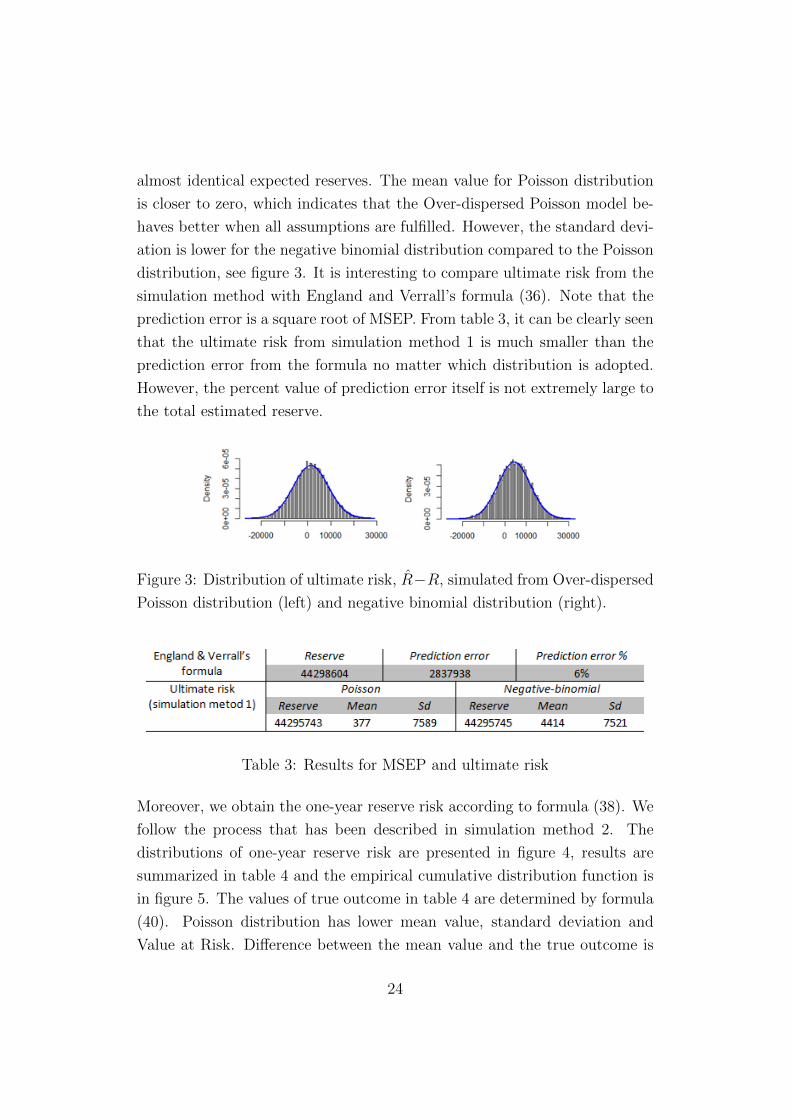
almost identical expected reserves. The mean value for Poisson distribution
is closer to zero, which indicates that the Over-dispersed Poisson model be-
haves better when all assumptions are fulfilled. However, the standard devi-
ation is lower for the negative binomial distribution compared to the Poisson
distribution, see figure 3. It is interesting to compare ultimate risk from the
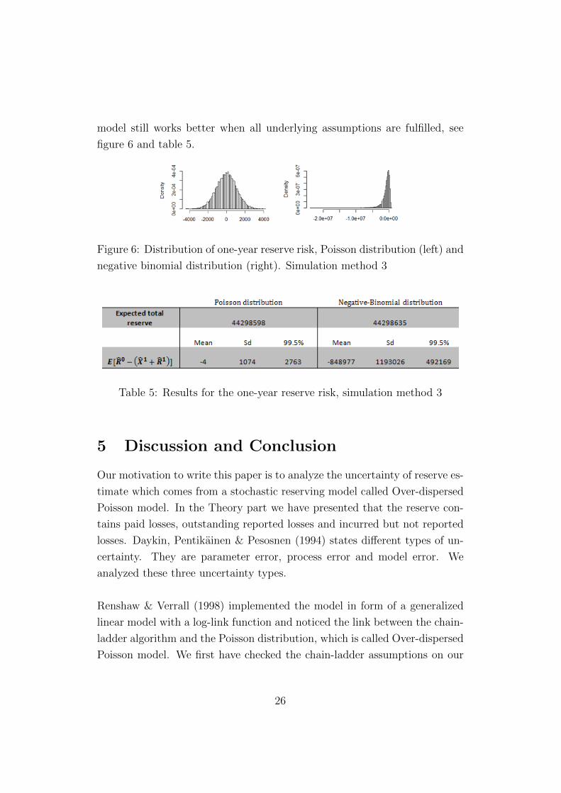
simulation method with England and Verrall’s formula (36). Note that the
prediction error is a square root of MSEP. From table 3, it can be clearly seen
that the ultimate risk from simulation method 1 is much smaller than the
prediction error from the formula no matter which distribution is adopted.
However, the percent value of prediction error itself is not extremely large to
the total estimated reserve.
Figure 3: Distribution of ultimate risk, R−R, simulated from Over-dispersed
Poisson distribution (left) and negative binomial distribution (right).
Table 3: Results for MSEP and ultimate risk
Moreover, we obtain the one-year reserve risk according to formula (38). We
follow the process that has been described in simulation method 2. The
distributions of one-year reserve risk are presented in figure 4, results are
summarized in table 4 and the empirical cumulative distribution function is
in figure 5. The values of true outcome in table 4 are determined by formula
(40). Poisson distribution has lower mean value, standard deviation and
Value at Risk. Difference between the mean value and the true outcome is
24

quite large for negative binomial distribution. Since the mean values from
both distributions are non positive, we have reserve losses. In summary, the
Over-dispersed Poisson model still behaves better when all assumptions are
fulfilled.
Figure 4: Distribution of one-year reserve risk simulated from Poisson distri-
bution (left) and negative binomial distribution (right). Simulation method
2
Table 4: Results for the one-year reserve risk, simulation method 2
Figure 5: Empirical cumulative distribution function of one-year reserve risk
simulated from Poisson distribution (left) and negative binomial distribution
(right)
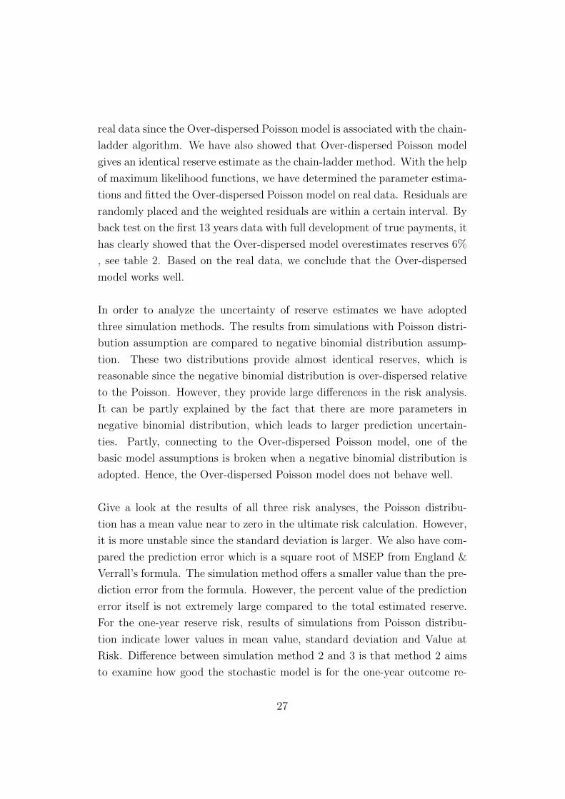
Finally, we adopt simulation method 3 to obtain the risk uncertainty. Re-
member, here the reserve R0 is not considered to be fixed. The reserving
25
model still works better when all underlying assumptions are fulfilled, see
figure 6 and table 5.
Figure 6: Distribution of one-year reserve risk, Poisson distribution (left) and
negative binomial distribution (right). Simulation method 3
Table 5: Results for the one-year reserve risk, simulation method 3
5 Discussion and Conclusion
Our motivation to write this paper is to analyze the uncertainty of reserve es-
timate which comes from a stochastic reserving model called Over-dispersed
Poisson model. In the Theory part we have presented that the reserve con-
tains paid losses, outstanding reported losses and incurred but not reported
losses. Daykin, Pentikainen & Pesosnen (1994) states different types of un-
certainty. They are parameter error, process error and model error. We
analyzed these three uncertainty types.
Renshaw & Verrall (1998) implemented the model in form of a generalized
linear model with a log-link function and noticed the link between the chain-
ladder algorithm and the Poisson distribution, which is called Over-dispersed
Poisson model. We first have checked the chain-ladder assumptions on our
26
real data since the Over-dispersed Poisson model is associated with the chain-
ladder algorithm. We have also showed that Over-dispersed Poisson model
gives an identical reserve estimate as the chain-ladder method. With the help
of maximum likelihood functions, we have determined the parameter estima-
tions and fitted the Over-dispersed Poisson model on real data. Residuals are
randomly placed and the weighted residuals are within a certain interval. By
back test on the first 13 years data with full development of true payments, it
has clearly showed that the Over-dispersed model overestimates reserves 6%
, see table 2. Based on the real data, we conclude that the Over-dispersed
model works well.
In order to analyze the uncertainty of reserve estimates we have adopted
three simulation methods. The results from simulations with Poisson distri-
bution assumption are compared to negative binomial distribution assump-
tion. These two distributions provide almost identical reserves, which is
reasonable since the negative binomial distribution is over-dispersed relative
to the Poisson. However, they provide large differences in the risk analysis.
It can be partly explained by the fact that there are more parameters in
negative binomial distribution, which leads to larger prediction uncertain-
ties. Partly, connecting to the Over-dispersed Poisson model, one of the
basic model assumptions is broken when a negative binomial distribution is
adopted. Hence, the Over-dispersed Poisson model does not behave well.
Give a look at the results of all three risk analyses, the Poisson distribu-
tion has a mean value near to zero in the ultimate risk calculation. However,
it is more unstable since the standard deviation is larger. We also have com-
pared the prediction error which is a square root of MSEP from England &
Verrall’s formula. The simulation method offers a smaller value than the pre-
diction error from the formula. However, the percent value of the prediction
error itself is not extremely large compared to the total estimated reserve.
For the one-year reserve risk, results of simulations from Poisson distribu-
tion indicate lower values in mean value, standard deviation and Value at
Risk. Difference between simulation method 2 and 3 is that method 2 aims
to examine how good the stochastic model is for the one-year outcome re-
27

serve risk. However, a stochastic model is not a indispensable condition in
simulation method 3, but we have simulated data and see how the expected
prediction of reserves behaves.
In summary, we have showed that the reserve risks behave better when the
underlying assumptions of Over-dispersed Poisson model are fulfilled. In
the other word, the Over-dispersed model works as expected given that the
underlying assumptions are fulfilled. The results can become poor if the
underlying assumptions are broken.
6 Limitations and future researches
There are several ways to extend and improve our analysis. First, the data in
our study is limited to payments due to the property of the insurance prod-
uct. One would have to include data of reserves in further researches. One
could investigate how different stresses on the estimated parameters affect
the reserve if the data of reserves is involved.
Secondly, Renshaw & Verrall (1998) assume the incremental payments are
Poisson distributed in the model. Beside the Poisson distribution, we have
also assumed and analyzed that the incremental payments are negative bi-
nomial distributed. Kremer (1982) used a log-normal distribution, which is
a most common distribution used for claims payments. Other distributions
could be analyzed in the further analysis.
28

7 References
References
[1] Dahl, P. (2003) Introduction to Reserving. Stockholms University
[2] Daykin, C. D., Pentikainen, T. & Pesosnen, M. (1994) Practical Risk
Theory for Actuaries. London: Chapman & Hall.
[3] England, P. D. & Verrall, R. J. (2002) Stochastic claims reserving in
general insurance. Institute of Actuaries and Faculty of Actuaries
[4] Gould, I. L. (2008) Stochastic chain-ladder models in nonlife insurance.
The University of Bergen
[5] Huang, J. & Wu, X. (2012) Stochastiv Claims Reserving in General In-
surance: Models and Methodologies. Department of Statistics and Ac-
tuarial Science, East China Normal University
[6] Kremer, E. (1982) IBNR-claims and the two-way model of ANOVA.
Scand. Act. J 1, 47-55.
[7] Mack, T. (1993a) Distribution-free calculation of the standard error of
chain ladder reserve estimates. ASTIN BULLETIN, 23:2.
[8] Mack, T. (1993b) Measuring the Variability of Chain Ladder Reserve
Estimates. The Casualty Actuarial Society
[9] Niman, P. (2007) Stochastic claims reserving of a Swedish life insurance
portfolio. The Swedish Actuarial Society.
[10] Ohlsson, E. & Lauzeningks, J. (2009). The one-year non-life insurance
risk. Insurance: Mathematics and Economics, 45(2):203 – 208.
[11] Pinheiro, P. J. R. & Andrade e Silva, J. M. & Centeno, M. L. (2000).
Bootstrap methodology in claim reserving. Centre for Applied Maths,
Forecasting & Economic Decision, ISEG Lisboa
29

[12] Renshaw, A. E. & Verrall, R.J. (1998) A stochastic model underlying
the chain-ladder technique. B.A.J.4,IV, 903-923.
[13] Rosenberg, P. S. (1990) A simple correlation of AIDS surveillance data
for reporting delays. J. AIDS, 3, 49-54.
[14] Wuthrich, M. V. (2015). Non-Life Insurance: Mathematics & Statistics.
Department of Mathematics, ETH
[15] Wuthrich, M. V., Merz, M. & Lysenko, N. (2007). Uncertainty in the
claims development result in the chain ladder method. ETH, Zurich
8 Appendix
Figure 7: Regression and residuals Ci2 against Ci1 (left) and weighted resid-
uals (right).
30

Figure 8: Regression and residuals Ci3 against Ci2 (left) and weighted resid-
uals (right).
Figure 9: Regression and residuals Ci4 against Ci3 (left) and weighted resid-
uals (right).
31

Figure 10: Regression and residuals Ci5 against Ci4 (left) and weighted resid-
uals (right).
Figure 11: Regression and residuals Ci6 against Ci5 (left) and weighted resid-
uals (right).
32
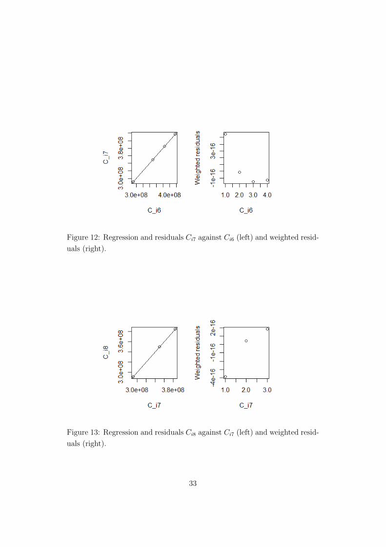
Figure 12: Regression and residuals Ci7 against Ci6 (left) and weighted resid-
uals (right).
Figure 13: Regression and residuals Ci8 against Ci7 (left) and weighted resid-
uals (right).
33

Figure 14: Regression and residuals Ci9 against Ci8 (left) and weighted resid-
uals (right).
Table 6: Development factors fik.
Table 7: Results of rank factor rik.
34

Table 8: Results of rank factor sik.
Table 9: Spearman’s rank coefficients Tk.
Table 10: Results of large rank, small rank and mean rank
35

Table 11: Results of expected value and variance of Zj
36