Embed Size (px)
Citation preview
Analysis of System Reports of Task 26 for Sensitivity of Parameters
A Report of IEA SHC - Task 26 Solar Combisystems December 2003 (revised February 2007)
Wolfgang Streicher Richard Heimrath Chris Bales
Analysis of System Reports of Task 26 for Sensitivity of Parameters
by
Wolfgang Streicher* and Richard Heimrath*
A technical report of Subtask C
*Institute of Thermal Engineering Graz University of Technology
Austria
IEA SHC – Task 26 – Solar Combisystems
3
Contents
1 INTRODUCTION AND METHODOLOGY 5
2 DESCRIPTIONS OF SYSTEMS ANALYZED 6
2.1 System #2 [6] 6 2.2 System #3a [7] 7 2.3 System #4 [8] 8 2.4 System #8 [9] 9 2.5 System #9b [10] 10 2.6 System #11 [11] 12 2.7 System #12 [12] 13 2.8 System #15 [13] 14 2.9 System #19 [14] 15
3 INFLUENCE OF CLIMATE AND HEAT LOAD (BUILDING TYPE) 16
4 INFLUENCE OF PARAMETERS CONCERNING COLLECTOR 21
4.1 Collector slope and azimuth 21 4.2 Collector size 22 4.3 Collector mass flow 23 4.4 Collector control settings 24
5 INFLUENCE OF PARAMETERS CONCERNING STORAGE 25
5.1 Storage volume 25 5.2 Combined collector size/store volume 26 5.3 Storage insulation 28 5.4 Size of heat exchangers 29 5.5 Position of components 30
5.5.1 Position of Inlet/Outlet pairs or heat exchangers 31
5.5.2 Position of temperature sensors 34
5.6 Mass flow from/to heat storage 35 5.7 Storage related control settings 37
6 INFLUENCE OF BOILER AND SH SYSTEM 38
6.1 Influence of boiler type and control 38 6.2 Influence of the SH system 42
7 GENERAL ANALYSIS AND CONCLUSION 43
7.1 Methodology 43 7.2 Results 44 7.3 Conclusion 48

IEA SHC – Task 26 – Solar Combisystems
4
8 REFERENCES 49
IEA SHC – Task 26 – Solar Combisystems
5
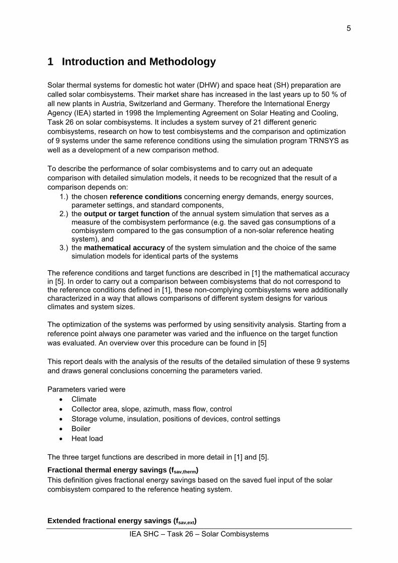
1 Introduction and Methodology Solar thermal systems for domestic hot water (DHW) and space heat (SH) preparation are called solar combisystems. Their market share has increased in the last years up to 50 % of all new plants in Austria, Switzerland and Germany. Therefore the International Energy Agency (IEA) started in 1998 the Implementing Agreement on Solar Heating and Cooling, Task 26 on solar combisystems. It includes a system survey of 21 different generic combisystems, research on how to test combisystems and the comparison and optimization of 9 systems under the same reference conditions using the simulation program TRNSYS as well as a development of a new comparison method. To describe the performance of solar combisystems and to carry out an adequate comparison with detailed simulation models, it needs to be recognized that the result of a comparison depends on:
1.) the chosen reference conditions concerning energy demands, energy sources, parameter settings, and standard components,
2.) the output or target function of the annual system simulation that serves as a measure of the combisystem performance (e.g. the saved gas consumptions of a combisystem compared to the gas consumption of a non-solar reference heating system), and
3.) the mathematical accuracy of the system simulation and the choice of the same simulation models for identical parts of the systems
The reference conditions and target functions are described in [1] the mathematical accuracy in [5]. In order to carry out a comparison between combisystems that do not correspond to the reference conditions defined in [1], these non-complying combisystems were additionally characterized in a way that allows comparisons of different system designs for various climates and system sizes. The optimization of the systems was performed by using sensitivity analysis. Starting from a reference point always one parameter was varied and the influence on the target function was evaluated. An overview over this procedure can be found in [5] This report deals with the analysis of the results of the detailed simulation of these 9 systems and draws general conclusions concerning the parameters varied. Parameters varied were
• Climate • Collector area, slope, azimuth, mass flow, control • Storage volume, insulation, positions of devices, control settings • Boiler • Heat load
The three target functions are described in more detail in [1] and [5].
Fractional thermal energy savings (fsav,therm) This definition gives fractional energy savings based on the saved fuel input of the solar combisystem compared to the reference heating system.
Extended fractional energy savings (fsav,ext)
IEA SHC – Task 26 – Solar Combisystems
6
In this definition, the above value takes into account the parasitic electricity Wpar used by the system.
Fractional savings indicator (fsi) This last definition includes also a penalty Qpenalty,red for not fulfilling the comfort criteria’s of domestic hot water (DHW) and room temperatures as described in [1] is added to the solar combisystem in the fractional energy savings.
2 Descriptions of systems analyzed The following 9 Systems were modelled within Subtask C of Task 26 and are described briefly in the following. Detailed descriptions can be found in [6] to [14]. A comparison using the FSC-method is given in [1] and [2]. Systems System #2 Klaus Ellehauge, Denmark [6] System #3a Philippe Papillon, David Chèze,,Clipsol, Aix-les-Bains, France [7] System #4 Louise Shivan Shah, Denmark [8] System #8 Jacques Bony, Thierry Pittet, EIVD, Yverdon-les-Bains, Switzerland
[9] System #9b Markus Peter, University Oslo, Norway [10] System #11 oil, gas Chris Bales, SERC, Borlänge, Sweden [11] System #12 base Chris Bales, SERC, Borlänge, Sweden [12] System #15 Dagmar Jaehnig, SOLVIS, Braunschweig, Germany [13] System #19 Richard Heimrath, IWT Graz, University of Technology, Austria [14]
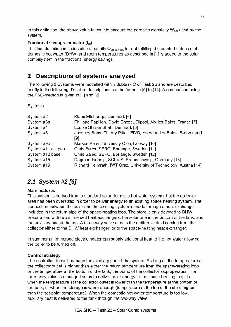
2.1 System #2 [6] Main features This system is derived from a standard solar domestic-hot-water system, but the collector area has been oversized in order to deliver energy to an existing space heating system. The connection between the solar and the existing system is made through a heat exchanger included in the return pipe of the space-heating loop. The store is only devoted to DHW preparation, with two immersed heat exchangers: the solar one in the bottom of the tank, and the auxiliary one at the top. A three-way valve directs the antifreeze fluid coming from the collector either to the DHW heat exchanger, or to the space-heating heat exchanger. In summer an immersed electric heater can supply additional heat to the hot water allowing the boiler to be turned off. Control strategy The controller doesn't manage the auxiliary part of the system. As long as the temperature at the collector outlet is higher than either the return temperature from the space-heating loop or the temperature at the bottom of the tank, the pump of the collector loop operates. The three-way valve is managed so as to deliver solar energy to the space-heating loop, i.e. when the temperature at the collector outlet is lower than the temperature at the bottom of the tank, or when the storage is warm enough (temperature at the top of the store higher than the set-point temperature). When the domestic-hot-water temperature is too low, auxiliary heat is delivered to the tank through the two-way valve.
IEA SHC – Task 26 – Solar Combisystems
7
Figure 1: System #2, hydraulic design
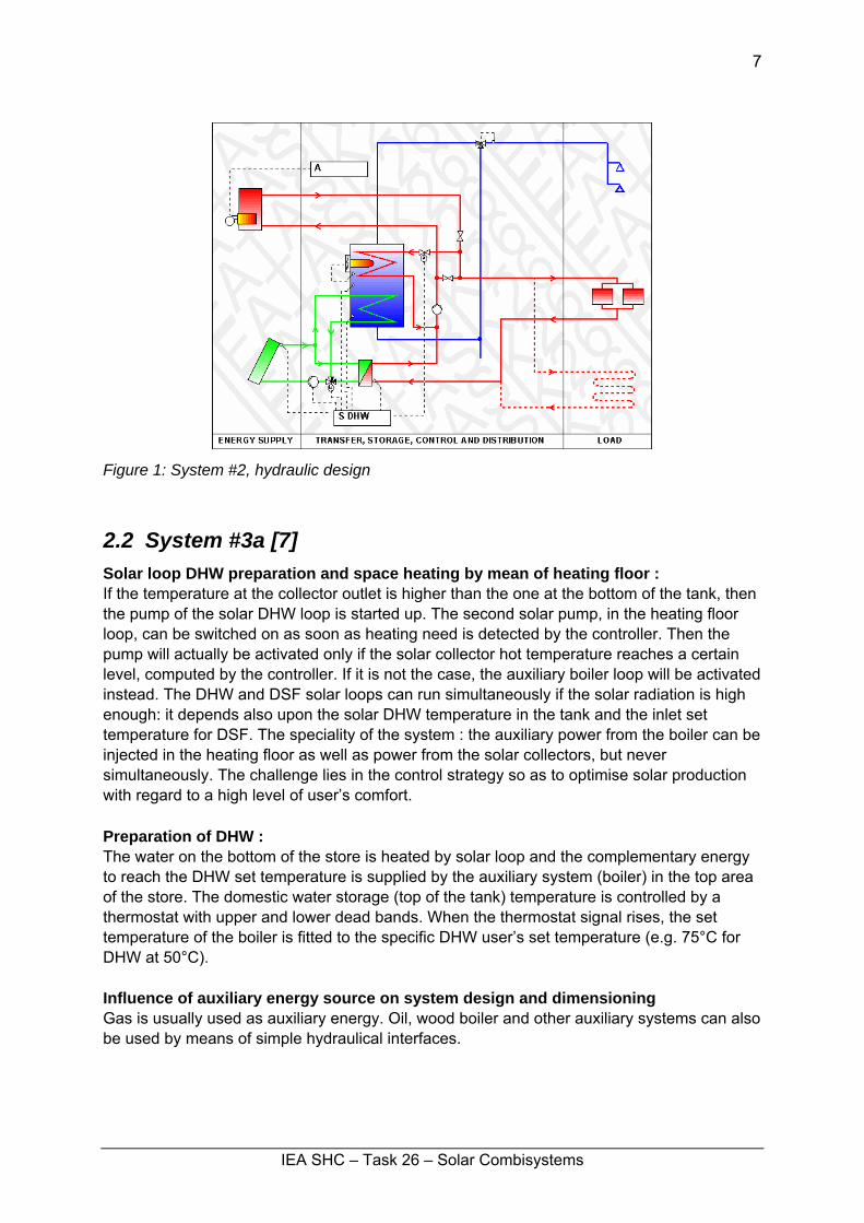
2.2 System #3a [7] Solar loop DHW preparation and space heating by mean of heating floor : If the temperature at the collector outlet is higher than the one at the bottom of the tank, then the pump of the solar DHW loop is started up. The second solar pump, in the heating floor loop, can be switched on as soon as heating need is detected by the controller. Then the pump will actually be activated only if the solar collector hot temperature reaches a certain level, computed by the controller. If it is not the case, the auxiliary boiler loop will be activated instead. The DHW and DSF solar loops can run simultaneously if the solar radiation is high enough: it depends also upon the solar DHW temperature in the tank and the inlet set temperature for DSF. The speciality of the system : the auxiliary power from the boiler can be injected in the heating floor as well as power from the solar collectors, but never simultaneously. The challenge lies in the control strategy so as to optimise solar production with regard to a high level of user’s comfort. Preparation of DHW : The water on the bottom of the store is heated by solar loop and the complementary energy to reach the DHW set temperature is supplied by the auxiliary system (boiler) in the top area of the store. The domestic water storage (top of the tank) temperature is controlled by a thermostat with upper and lower dead bands. When the thermostat signal rises, the set temperature of the boiler is fitted to the specific DHW user’s set temperature (e.g. 75°C for DHW at 50°C). Influence of auxiliary energy source on system design and dimensioning Gas is usually used as auxiliary energy. Oil, wood boiler and other auxiliary systems can also be used by means of simple hydraulical interfaces.
IEA SHC – Task 26 – Solar Combisystems
8
Figure 2: System #3a, hydraulic design
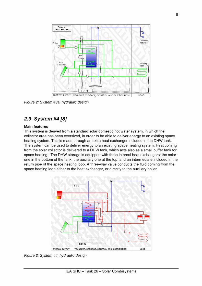
2.3 System #4 [8] Main features This system is derived from a standard solar domestic hot water system, in which the collector area has been oversized, in order to be able to deliver energy to an existing space heating system. This is made through an extra heat exchanger included in the DHW tank. The system can be used to deliver energy to an existing space heating system. Heat coming from the solar collector is delivered to a DHW tank, which acts also as a small buffer tank for space heating. The DHW storage is equipped with three internal heat exchangers: the solar one in the bottom of the tank, the auxiliary one at the top, and an intermediate included in the return pipe of the space heating loop. A three-way valve conducts the fluid coming from the space heating loop either to the heat exchanger, or directly to the auxiliary boiler.
ENERGY SUPPLY TRANSFER, STORAGE, CONTROL AND DISTRIBUTION LOAD
M
M
S DHW
A H1
Figure 3: System #4, hydraulic design
IEA SHC – Task 26 – Solar Combisystems
9
Heat management philosophy The controller does not manage the auxiliary part of the system. If the temperature at the collector outlet is higher than the temperature at the bottom of the tank, the pump of the solar loop works. The three-way valve is managed so as to deliver solar energy to the space heating loop, i.e. when the temperature in the middle of the tank is higher than the temperature at the return temperature from the space heating loop. When the hot water temperature is too low, auxiliary heat is delivered to the tank through the three-way valve. Specific aspects Solar heat used for space heating is stored in the domestic hot water tank. Influence of auxiliary energy source on system design and dimensioning This system can work with any auxiliary energy (gas, fuel, wood, district heating). It could be also used with separate electric radiators.
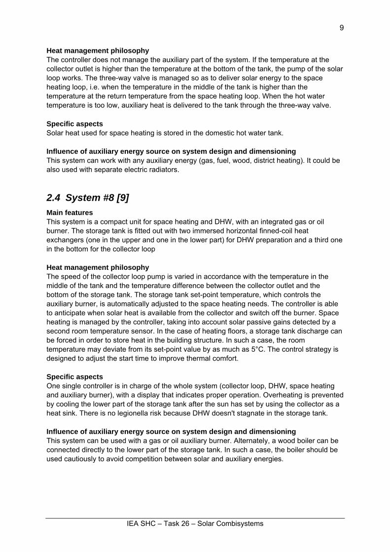
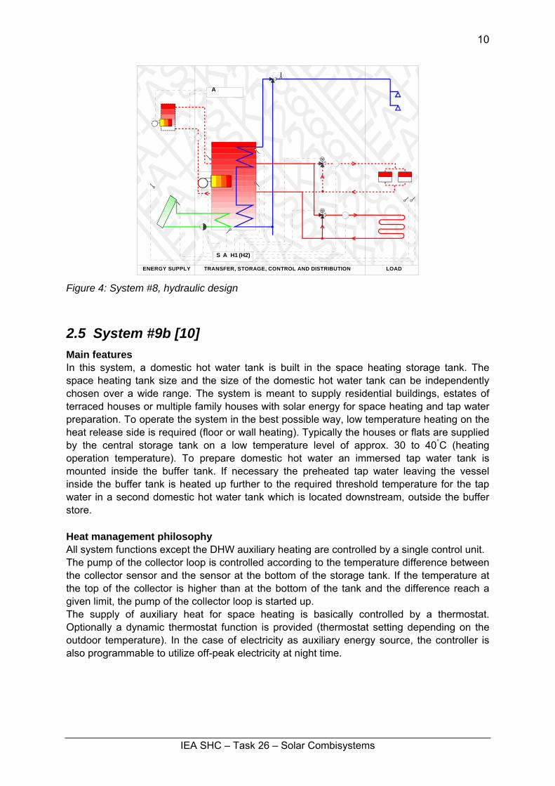
2.4 System #8 [9] Main features This system is a compact unit for space heating and DHW, with an integrated gas or oil burner. The storage tank is fitted out with two immersed horizontal finned-coil heat exchangers (one in the upper and one in the lower part) for DHW preparation and a third one in the bottom for the collector loop Heat management philosophy The speed of the collector loop pump is varied in accordance with the temperature in the middle of the tank and the temperature difference between the collector outlet and the bottom of the storage tank. The storage tank set-point temperature, which controls the auxiliary burner, is automatically adjusted to the space heating needs. The controller is able to anticipate when solar heat is available from the collector and switch off the burner. Space heating is managed by the controller, taking into account solar passive gains detected by a second room temperature sensor. In the case of heating floors, a storage tank discharge can be forced in order to store heat in the building structure. In such a case, the room temperature may deviate from its set-point value by as much as 5°C. The control strategy is designed to adjust the start time to improve thermal comfort. Specific aspects One single controller is in charge of the whole system (collector loop, DHW, space heating and auxiliary burner), with a display that indicates proper operation. Overheating is prevented by cooling the lower part of the storage tank after the sun has set by using the collector as a heat sink. There is no legionella risk because DHW doesn't stagnate in the storage tank. Influence of auxiliary energy source on system design and dimensioning This system can be used with a gas or oil auxiliary burner. Alternately, a wood boiler can be connected directly to the lower part of the storage tank. In such a case, the boiler should be used cautiously to avoid competition between solar and auxiliary energies.
IEA SHC – Task 26 – Solar Combisystems
10
H1
ENERGY SUPPLY TRANSFER, STORAGE, CONTROL AND DISTRIBUTION LOAD
M
M
S A H1 (H2)
A
Figure 4: System #8, hydraulic design
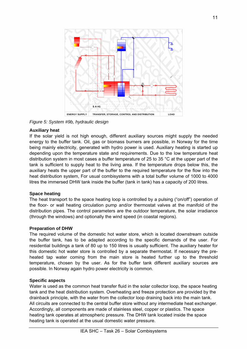
2.5 System #9b [10] Main features In this system, a domestic hot water tank is built in the space heating storage tank. The space heating tank size and the size of the domestic hot water tank can be independently chosen over a wide range. The system is meant to supply residential buildings, estates of terraced houses or multiple family houses with solar energy for space heating and tap water preparation. To operate the system in the best possible way, low temperature heating on the heat release side is required (floor or wall heating). Typically the houses or flats are supplied by the central storage tank on a low temperature level of approx. 30 to 40°C (heating operation temperature). To prepare domestic hot water an immersed tap water tank is mounted inside the buffer tank. If necessary the preheated tap water leaving the vessel inside the buffer tank is heated up further to the required threshold temperature for the tap water in a second domestic hot water tank which is located downstream, outside the buffer store. Heat management philosophy All system functions except the DHW auxiliary heating are controlled by a single control unit. The pump of the collector loop is controlled according to the temperature difference between the collector sensor and the sensor at the bottom of the storage tank. If the temperature at the top of the collector is higher than at the bottom of the tank and the difference reach a given limit, the pump of the collector loop is started up. The supply of auxiliary heat for space heating is basically controlled by a thermostat. Optionally a dynamic thermostat function is provided (thermostat setting depending on the outdoor temperature). In the case of electricity as auxiliary energy source, the controller is also programmable to utilize off-peak electricity at night time.
IEA SHC – Task 26 – Solar Combisystems
11
ENERGY SUPPLY TRANSFER, STORAGE, CONTROL AND DISTRIBUTION LOAD
M
S A H1
Figure 5: System #9b, hydraulic design
Auxiliary heat If the solar yield is not high enough, different auxiliary sources might supply the needed energy to the buffer tank. Oil, gas or biomass burners are possible, in Norway for the time being mainly electricity, generated with hydro power is used. Auxiliary heating is started up depending upon the temperature state and requirements. Due to the low temperature heat distribution system in most cases a buffer temperature of 25 to 35 °C at the upper part of the tank is sufficient to supply heat to the living area. If the temperature drops below this, the auxiliary heats the upper part of the buffer to the required temperature for the flow into the heat distribution system, For usual combisystems with a total buffer volume of 1000 to 4000 litres the immersed DHW tank inside the buffer (tank in tank) has a capacity of 200 litres. Space heating The heat transport to the space heating loop is controlled by a pulsing (“on/off”) operation of the floor- or wall heating circulation pump and/or thermostat valves at the manifold of the distribution pipes. The control parameters are the outdoor temperature, the solar irradiance (through the windows) and optionally the wind speed (in coastal regions). Preparation of DHW The required volume of the domestic hot water store, which is located downstream outside the buffer tank, has to be adapted according to the specific demands of the user. For residential buildings a tank of 80 up to 150 litres is usually sufficient. The auxiliary heater for this domestic hot water store is controlled by a separate thermostat. If necessary the pre-heated tap water coming from the main store is heated further up to the threshold temperature, chosen by the user. As for the buffer tank different auxiliary sources are possible. In Norway again hydro power electricity is common. Specific aspects Water is used as the common heat transfer fluid in the solar collector loop, the space heating tank and the heat distribution system. Overheating and freeze protection are provided by the drainback principle, with the water from the collector loop draining back into the main tank. All circuits are connected to the central buffer store without any intermediate heat exchanger. Accordingly, all components are made of stainless steel, copper or plastics. The space heating tank operates at atmospheric pressure. The DHW tank located inside the space heating tank is operated at the usual domestic water pressure.
IEA SHC – Task 26 – Solar Combisystems
12
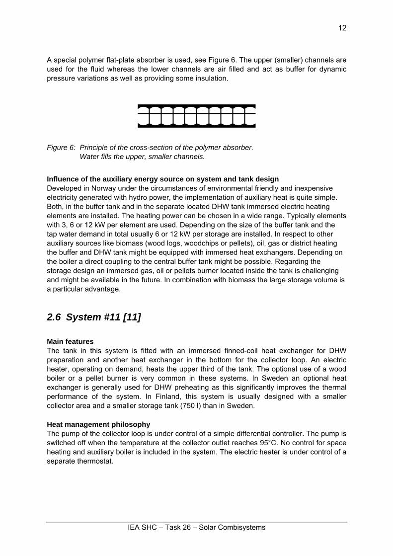
A special polymer flat-plate absorber is used, see Figure 6. The upper (smaller) channels are used for the fluid whereas the lower channels are air filled and act as buffer for dynamic pressure variations as well as providing some insulation.
Figure 6: Principle of the cross-section of the polymer absorber. Water fills the upper, smaller channels.
Influence of the auxiliary energy source on system and tank design Developed in Norway under the circumstances of environmental friendly and inexpensive electricity generated with hydro power, the implementation of auxiliary heat is quite simple. Both, in the buffer tank and in the separate located DHW tank immersed electric heating elements are installed. The heating power can be chosen in a wide range. Typically elements with 3, 6 or 12 kW per element are used. Depending on the size of the buffer tank and the tap water demand in total usually 6 or 12 kW per storage are installed. In respect to other auxiliary sources like biomass (wood logs, woodchips or pellets), oil, gas or district heating the buffer and DHW tank might be equipped with immersed heat exchangers. Depending on the boiler a direct coupling to the central buffer tank might be possible. Regarding the storage design an immersed gas, oil or pellets burner located inside the tank is challenging and might be available in the future. In combination with biomass the large storage volume is a particular advantage.
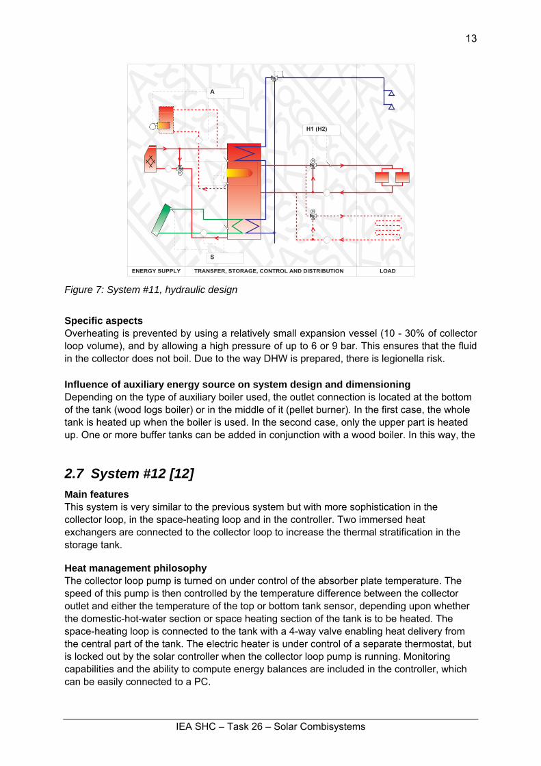
2.6 System #11 [11] Main features The tank in this system is fitted with an immersed finned-coil heat exchanger for DHW preparation and another heat exchanger in the bottom for the collector loop. An electric heater, operating on demand, heats the upper third of the tank. The optional use of a wood boiler or a pellet burner is very common in these systems. In Sweden an optional heat exchanger is generally used for DHW preheating as this significantly improves the thermal performance of the system. In Finland, this system is usually designed with a smaller collector area and a smaller storage tank (750 l) than in Sweden. Heat management philosophy The pump of the collector loop is under control of a simple differential controller. The pump is switched off when the temperature at the collector outlet reaches 95°C. No control for space heating and auxiliary boiler is included in the system. The electric heater is under control of a separate thermostat.
IEA SHC – Task 26 – Solar Combisystems
13
� � � � � � � � � � � � � � � � � � � � � � � � � � � � � � � � � � � � � � � � � � � � � � � � � � � �
�
�
�
�
� � � � � � �
Figure 7: System #11, hydraulic design
Specific aspects Overheating is prevented by using a relatively small expansion vessel (10 - 30% of collector loop volume), and by allowing a high pressure of up to 6 or 9 bar. This ensures that the fluid in the collector does not boil. Due to the way DHW is prepared, there is legionella risk. Influence of auxiliary energy source on system design and dimensioning Depending on the type of auxiliary boiler used, the outlet connection is located at the bottom of the tank (wood logs boiler) or in the middle of it (pellet burner). In the first case, the whole tank is heated up when the boiler is used. In the second case, only the upper part is heated up. One or more buffer tanks can be added in conjunction with a wood boiler. In this way, the
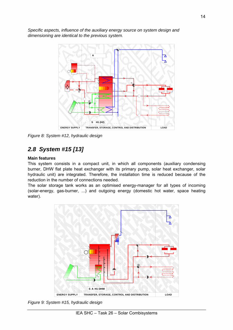
2.7 System #12 [12] Main features This system is very similar to the previous system but with more sophistication in the collector loop, in the space-heating loop and in the controller. Two immersed heat exchangers are connected to the collector loop to increase the thermal stratification in the storage tank. Heat management philosophy The collector loop pump is turned on under control of the absorber plate temperature. The speed of this pump is then controlled by the temperature difference between the collector outlet and either the temperature of the top or bottom tank sensor, depending upon whether the domestic-hot-water section or space heating section of the tank is to be heated. The space-heating loop is connected to the tank with a 4-way valve enabling heat delivery from the central part of the tank. The electric heater is under control of a separate thermostat, but is locked out by the solar controller when the collector loop pump is running. Monitoring capabilities and the ability to compute energy balances are included in the controller, which can be easily connected to a PC.
IEA SHC – Task 26 – Solar Combisystems
14
Specific aspects, influence of the auxiliary energy source on system design and dimensioning are identical to the previous system.
ENERGY SUPPLY TRANSFER, STORAGE, CONTROL AND DISTRIBUTION LOAD
M
S H1 (H2)
A
Figure 8: System #12, hydraulic design
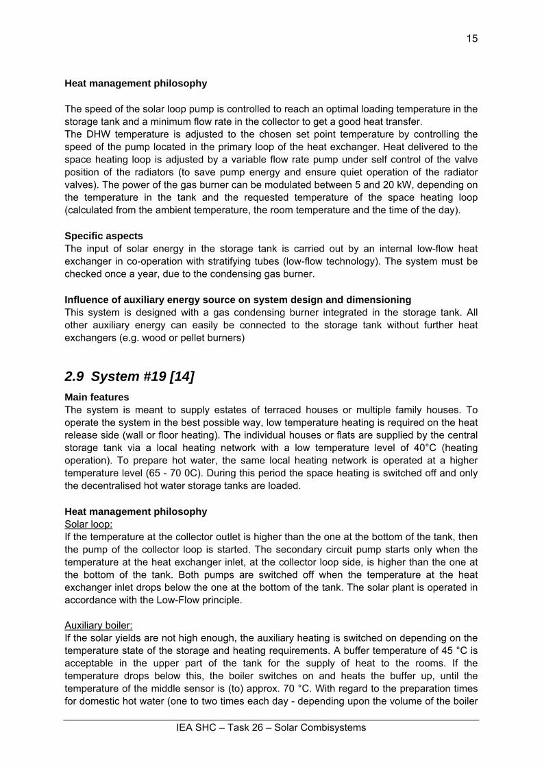
2.8 System #15 [13] Main features This system consists in a compact unit, in which all components (auxiliary condensing burner, DHW flat plate heat exchanger with its primary pump, solar heat exchanger, solar hydraulic unit) are integrated. Therefore, the installation time is reduced because of the reduction in the number of connections needed. The solar storage tank works as an optimised energy-manager for all types of incoming (solar-energy, gas-burner, ...) and outgoing energy (domestic hot water, space heating water).
ENERGY SUPPLY TRANSFER, STORAGE, CONTROL AND DISTRIBUTION LOAD
M
S A H1 DHW
Figure 9: System #15, hydraulic design
IEA SHC – Task 26 – Solar Combisystems
15
Heat management philosophy The speed of the solar loop pump is controlled to reach an optimal loading temperature in the storage tank and a minimum flow rate in the collector to get a good heat transfer. The DHW temperature is adjusted to the chosen set point temperature by controlling the speed of the pump located in the primary loop of the heat exchanger. Heat delivered to the space heating loop is adjusted by a variable flow rate pump under self control of the valve position of the radiators (to save pump energy and ensure quiet operation of the radiator valves). The power of the gas burner can be modulated between 5 and 20 kW, depending on the temperature in the tank and the requested temperature of the space heating loop (calculated from the ambient temperature, the room temperature and the time of the day). Specific aspects The input of solar energy in the storage tank is carried out by an internal low-flow heat exchanger in co-operation with stratifying tubes (low-flow technology). The system must be checked once a year, due to the condensing gas burner. Influence of auxiliary energy source on system design and dimensioning This system is designed with a gas condensing burner integrated in the storage tank. All other auxiliary energy can easily be connected to the storage tank without further heat exchangers (e.g. wood or pellet burners)
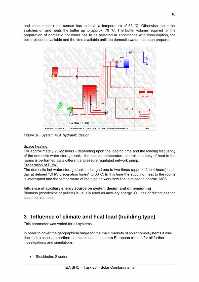
2.9 System #19 [14] Main features The system is meant to supply estates of terraced houses or multiple family houses. To operate the system in the best possible way, low temperature heating is required on the heat release side (wall or floor heating). The individual houses or flats are supplied by the central storage tank via a local heating network with a low temperature level of 40°C (heating operation). To prepare hot water, the same local heating network is operated at a higher temperature level (65 - 70 0C). During this period the space heating is switched off and only the decentralised hot water storage tanks are loaded. Heat management philosophy Solar loop: If the temperature at the collector outlet is higher than the one at the bottom of the tank, then the pump of the collector loop is started. The secondary circuit pump starts only when the temperature at the heat exchanger inlet, at the collector loop side, is higher than the one at the bottom of the tank. Both pumps are switched off when the temperature at the heat exchanger inlet drops below the one at the bottom of the tank. The solar plant is operated in accordance with the Low-Flow principle. Auxiliary boiler: If the solar yields are not high enough, the auxiliary heating is switched on depending on the temperature state of the storage and heating requirements. A buffer temperature of 45 °C is acceptable in the upper part of the tank for the supply of heat to the rooms. If the temperature drops below this, the boiler switches on and heats the buffer up, until the temperature of the middle sensor is (to) approx. 70 °C. With regard to the preparation times for domestic hot water (one to two times each day - depending upon the volume of the boiler
IEA SHC – Task 26 – Solar Combisystems
16
and consumption) this sensor has to have a temperature of 65 °C. Otherwise the boiler switches on and heats the buffer up to approx. 70 °C. The buffer volume required for the preparation of domestic hot water has to be selected in accordance with consumption, the boiler pipeline available and the time available until the domestic water has been prepared.
ENERGY SUPPLY TRANSFER, STORAGE, CONTROL AND DISTRIBUTION LOAD
S A H1 (H2)DHW
Figure 10: System #19, hydraulic design
Space heating: For approximately 20-22 hours - depending upon the loading time and the loading frequency of the domestic water storage tank - the outside temperature controlled supply of heat to the rooms is performed via a differential pressure regulated network pump. Preparation of DHW: The domestic hot water storage tank is charged one to two times (approx. 2 to 4 hours) each day at defined "DHW preparation times" to 60°C. In this time the supply of heat to the rooms is interrupted and the temperature of the pipe network flow line is raised to approx. 65°C. Influence of auxiliary energy source on system design and dimensioning Biomass (woodchips or pellets) is usually used as auxiliary energy. Oil, gas or district heating could be also used.
3 Influence of climate and heat load (building type) This parameter was varied for all systems In order to cover the geographical range for the main markets of solar combisystems it was decided to choose a northern, a middle and a southern European climate for all further investigations and simulations:
• Stockholm, Sweden
IEA SHC – Task 26 – Solar Combisystems
17
• Zurich, Switzerland • Carpentras, France
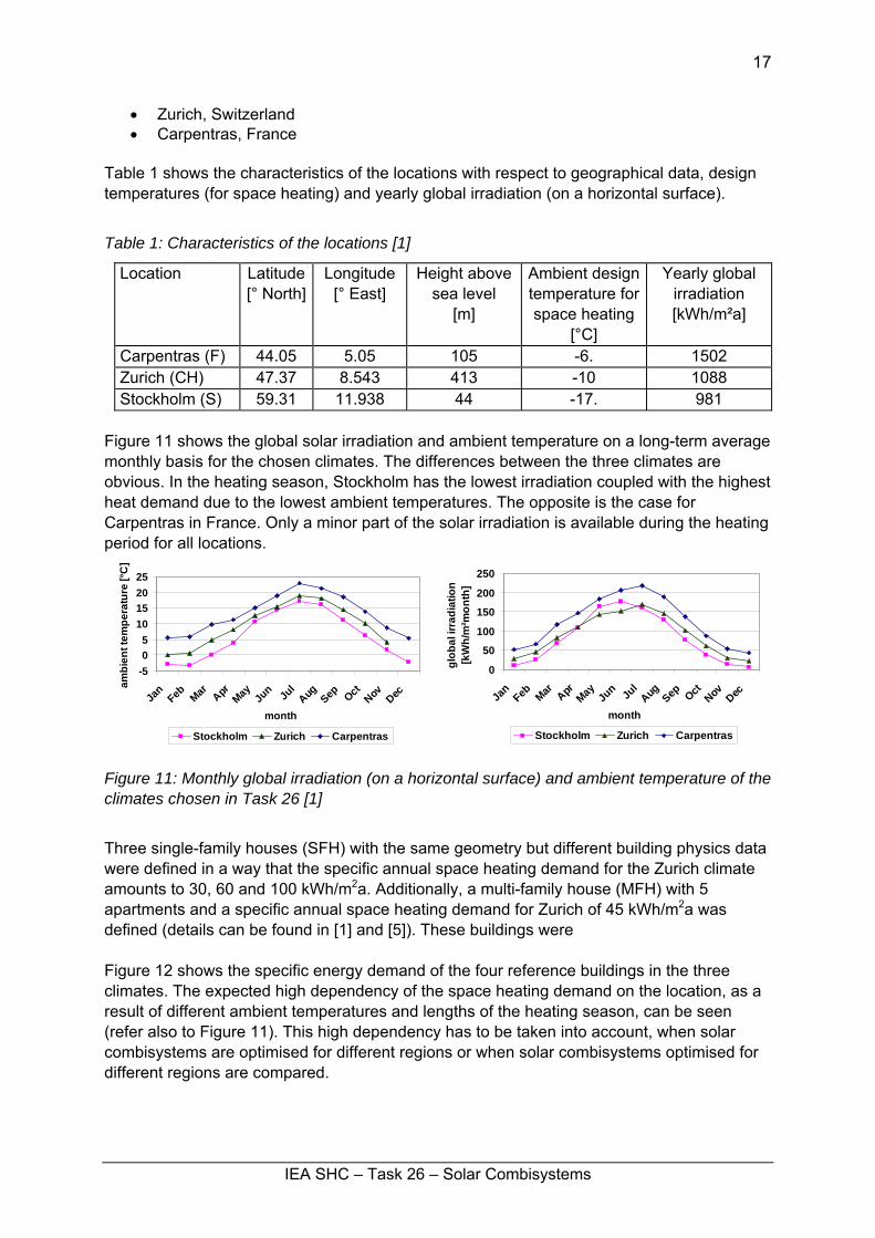
Table 1 shows the characteristics of the locations with respect to geographical data, design temperatures (for space heating) and yearly global irradiation (on a horizontal surface).
Table 1: Characteristics of the locations [1]
Location Latitude [° North]
Longitude[° East]
Height above sea level
[m]
Ambient design temperature for space heating
[°C]
Yearly global irradiation [kWh/m²a]
Carpentras (F) 44.05 5.05 105 -6. 1502 Zurich (CH) 47.37 8.543 413 -10 1088 Stockholm (S) 59.31 11.938 44 -17. 981
Figure 11 shows the global solar irradiation and ambient temperature on a long-term average monthly basis for the chosen climates. The differences between the three climates are obvious. In the heating season, Stockholm has the lowest irradiation coupled with the highest heat demand due to the lowest ambient temperatures. The opposite is the case for Carpentras in France. Only a minor part of the solar irradiation is available during the heating period for all locations.
-505
10152025
Jan
Feb Mar AprMay Ju
n Jul
Aug Sep OctNov Dec
month
ambi
ent t
empe
ratu
re [°
C]
Stockholm Zurich Carpentras
0
50
100
150
200
250
Jan
Feb Mar AprMay Ju
n Jul
Aug Sep OctNov Dec
month
glob
al ir
radi
atio
n [k
Wh/
m²m
onth
]
Stockholm Zurich Carpentras
Figure 11: Monthly global irradiation (on a horizontal surface) and ambient temperature of the climates chosen in Task 26 [1]
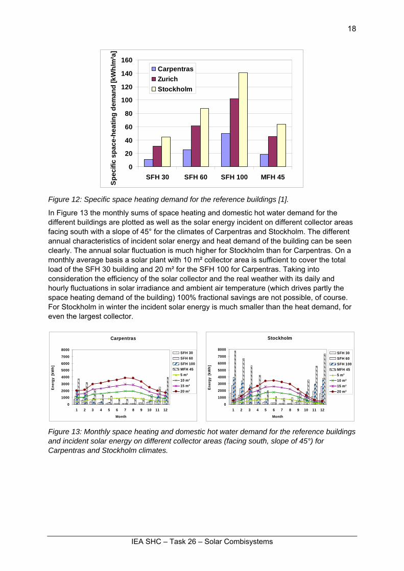
Three single-family houses (SFH) with the same geometry but different building physics data were defined in a way that the specific annual space heating demand for the Zurich climate amounts to 30, 60 and 100 kWh/m2a. Additionally, a multi-family house (MFH) with 5 apartments and a specific annual space heating demand for Zurich of 45 kWh/m2a was defined (details can be found in [1] and [5]). These buildings were Figure 12 shows the specific energy demand of the four reference buildings in the three climates. The expected high dependency of the space heating demand on the location, as a result of different ambient temperatures and lengths of the heating season, can be seen (refer also to Figure 11). This high dependency has to be taken into account, when solar combisystems are optimised for different regions or when solar combisystems optimised for different regions are compared.
IEA SHC – Task 26 – Solar Combisystems
18
0
20
40
60
80
100
120
140
160
SFH 30 SFH 60 SFH 100 MFH 45
Spec
ific
spac
e-he
atin
g de
man
d [k
Wh/
m²a
]
CarpentrasZurichStockholm
Figure 12: Specific space heating demand for the reference buildings [1].
In Figure 13 the monthly sums of space heating and domestic hot water demand for the different buildings are plotted as well as the solar energy incident on different collector areas facing south with a slope of 45° for the climates of Carpentras and Stockholm. The different annual characteristics of incident solar energy and heat demand of the building can be seen clearly. The annual solar fluctuation is much higher for Stockholm than for Carpentras. On a monthly average basis a solar plant with 10 m² collector area is sufficient to cover the total load of the SFH 30 building and 20 m² for the SFH 100 for Carpentras. Taking into consideration the efficiency of the solar collector and the real weather with its daily and hourly fluctuations in solar irradiance and ambient air temperature (which drives partly the space heating demand of the building) 100% fractional savings are not possible, of course. For Stockholm in winter the incident solar energy is much smaller than the heat demand, for even the largest collector.
Carpentras
0
1000
2000
3000
4000
5000
6000
7000
8000
1 2 3 4 5 6 7 8 9 10 11 12
Month
Ener
gy [
kWh]
SFH 30SFH 60SFH 100MFH 455 m²10 m²15 m²20 m²
Stockholm
0
1000
2000
3000
4000
5000
6000
7000
8000
1 2 3 4 5 6 7 8 9 10 11 12
Month
Ener
gy [
kWh]
SFH 30SFH 60SFH 100MFH 455 m²10 m²15 m²20 m²
Figure 13: Monthly space heating and domestic hot water demand for the reference buildings and incident solar energy on different collector areas (facing south, slope of 45°) for Carpentras and Stockholm climates.
IEA SHC – Task 26 – Solar Combisystems
19
0%
10%
20%
30%
40%
50%
100 kWh/m2.a 60 kWh/m2.a 30 kWh/m2.a
Climate and Load
f sa
ve,t
h
Carpentras
Zurich
Stockholm
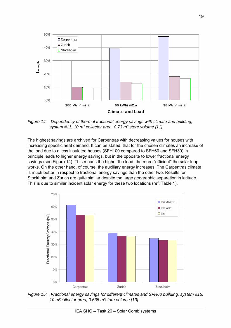
Figure 14: Dependency of thermal fractional energy savings with climate and building,
system #11, 10 m² collector area, 0.73 m³ store volume [11].
The highest savings are archived for Carpentras with decreasing values for houses with increasing specific heat demand. It can be stated, that for the chosen climates an increase of the load due to a less insulated houses (SFH100 compared to SFH60 and SFH30) in principle leads to higher energy savings, but in the opposite to lower fractional energy savings (see Figure 14). This means the higher the load, the more "efficient" the solar loop works. On the other hand, of course, the auxiliary energy increases. The Carpentras climate is much better in respect to fractional energy savings than the other two. Results for Stockholm and Zurich are quite similar despite the large geographic separation in latitude. This is due to similar incident solar energy for these two locations (ref. Table 1).
0%
10%
20%
30%
40%
50%
60%
70%
Carpentras Zurich Stockholm
Frac
tiona
l Ene
rgy
Savi
ngs
/[%
]
Fsavtherm
Fsavext
Fsi
Figure 15: Fractional energy savings for different climates and SFH60 building, system #15,
10 m²collector area, 0.635 m³store volume [13]
IEA SHC – Task 26 – Solar Combisystems
20
In Figure 15 the different fractional energy savings for system #15 are shown. The difference between Stockholm and Zurich climate is a little bigger compared to Figure 14 because the fractional energy savings is higher. For low fractional energy savings, most of the solar energy is used in summer for domestic hot water preparation. As shown in Figure 13 the incident solar energy is even a bit higher in Stockholm compared to Zurich. Amazingly system #11 has far lower fractional savings compared to system #15 although collector area (and type) and store volume are similar. The main difference lays in the boiler type of the two systems. Whereas system #11 uses an oil boiler with lower efficiency than the boiler for the reference building the gas condensing boiler of system #15 has a significantly higher efficiency than the boiler of the reference building. Additionally the positions and size of the heat exchangers, the store insulation and the control settings were not optimal for system #11. System #15 on the other hand has been optimized already in most of these aspects. An optimized version of system #11 using a gas boiler increases the fractional energy savings for example from 10 % (Stockholm climate, SFH 100) to 25 % (ref. also to Figure 43), which is still less but much closer to system #15. Further advantages of system #15 lay in the stratified charge of the storage compared to the internal heat exchanger of system #11 and the different DHW production (external heat exchanger system #15 compared to internal heat exchanger of system #11, which disturbes the stratification in the tank).
Energy Demand and Solar Fraction [%] - Single Family HouseBase Case, Collector Area: 20 m², Store Volume: 1,5 m³
0
5.000
10.000
15.000
20.000
25.000
30.000
30 60 100 30 60 100 30 60 100
Specific Energy Demand (thermal) of a Single Family House [kWh/(m²a)]
Tota
l Ene
rgy,
Q-th
erm
al [k
Wh]
Q-Solar
Q-Auxiliary
Stockholm
Zurich
Carpentras
35,6%
25,9%
21,1%
47,8%
33,8%
22,5%
83,7%
68,0%
53,7%
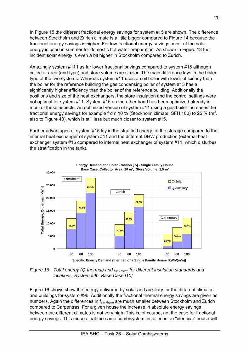
Figure 16 Total energy (Q-thermal) and fsav,therm for different insulation standards and
locations. System #9b: Base Case [10]
Figure 16 shows show the energy delivered by solar and auxiliary for the different climates and buildings for system #9b. Additionally the fractional thermal energy savings are given as numbers. Again the differences in fsav,therm are much smaller between Stockholm and Zurich compared to Carpentras. For a given house the increase in absolute energy savings between the different climates is not very high. This is, of course, not the case for fractional energy savings. This means that the same combisystem installed in an "identical" house will
IEA SHC – Task 26 – Solar Combisystems
21
provide more or less the same energy savings and consequently the same gas or oil savings. In other words, it is equal profitable to install combisystems anywhere in Europe.
4 Influence of parameters concerning collector
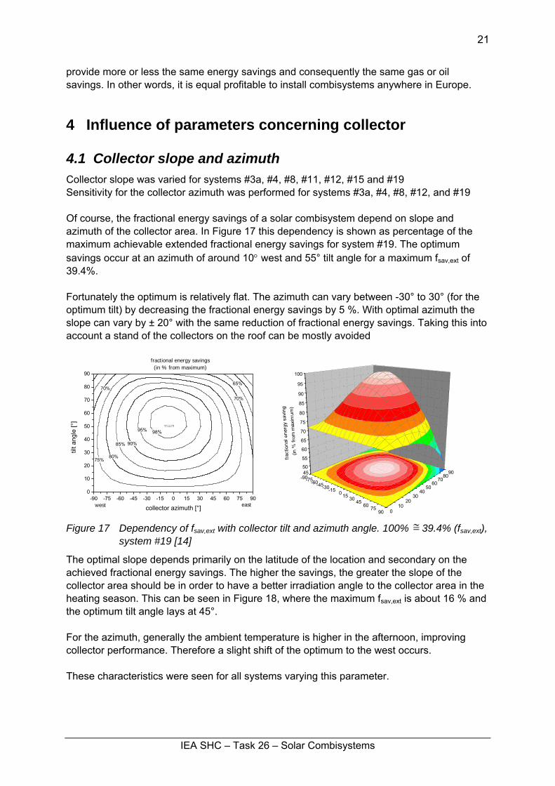
4.1 Collector slope and azimuth Collector slope was varied for systems #3a, #4, #8, #11, #12, #15 and #19 Sensitivity for the collector azimuth was performed for systems #3a, #4, #8, #12, and #19 Of course, the fractional energy savings of a solar combisystem depend on slope and azimuth of the collector area. In Figure 17 this dependency is shown as percentage of the maximum achievable extended fractional energy savings for system #19. The optimum savings occur at an azimuth of around 10° west and 55° tilt angle for a maximum fsav,ext of 39.4%. Fortunately the optimum is relatively flat. The azimuth can vary between -30° to 30° (for the optimum tilt) by decreasing the fractional energy savings by 5 %. With optimal azimuth the slope can vary by ± 20° with the same reduction of fractional energy savings. Taking this into account a stand of the collectors on the roof can be mostly avoided
75%
70%
65%70%
80%
85% 90%
95% 98%
-90 -75 -60 -45 -30 -15 0 15 30 45 60 75 900
10
20
30
40
50
60
70
80
90
east
tilt a
ngle
[°]
collector azimuth [°]west
fractional energy savings (in % from maximum)
-90-75-60-45-30-15 0 15 30 4560 75
90
4550
55
60
65
70
75
80
85
90
95
100
010
2030
4050
6070
8090
Figure 17 Dependency of fsav,ext with collector tilt and azimuth angle. 100% ≅ 39.4% (fsav,ext),
system #19 [14]
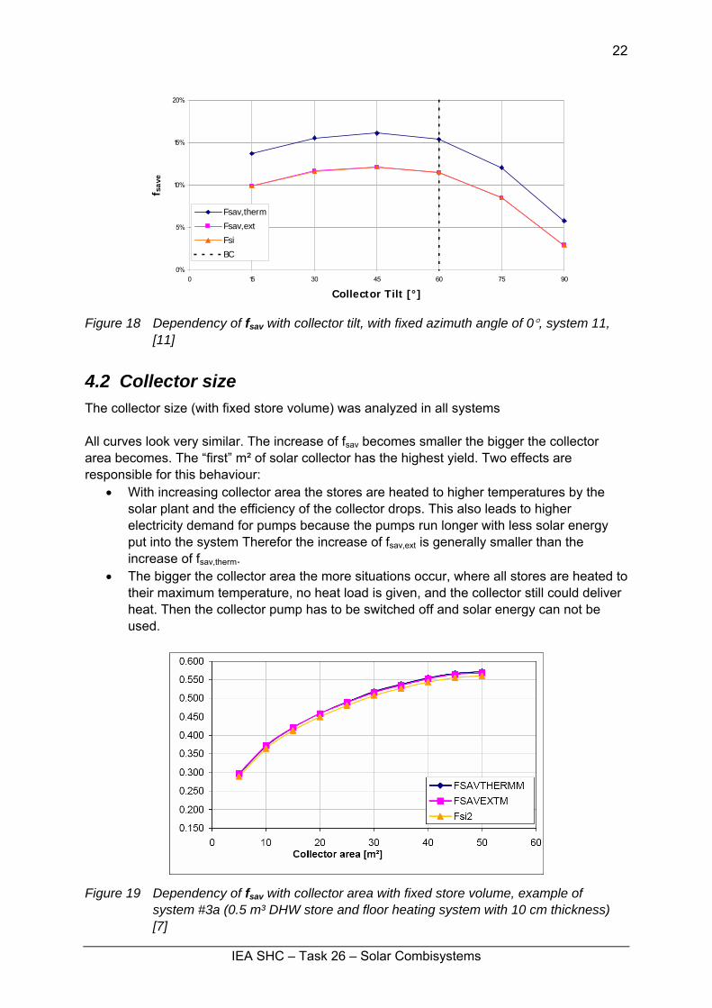
The optimal slope depends primarily on the latitude of the location and secondary on the achieved fractional energy savings. The higher the savings, the greater the slope of the collector area should be in order to have a better irradiation angle to the collector area in the heating season. This can be seen in Figure 18, where the maximum fsav,ext is about 16 % and the optimum tilt angle lays at 45°. For the azimuth, generally the ambient temperature is higher in the afternoon, improving collector performance. Therefore a slight shift of the optimum to the west occurs. These characteristics were seen for all systems varying this parameter.
IEA SHC – Task 26 – Solar Combisystems
22
0%
5%
10%
15%
20%
0 15 30 45 60 75 90
Collector Tilt [°]
f sav
e
Fsav,therm
Fsav,ext
Fsi
BC
Figure 18 Dependency of fsav with collector tilt, with fixed azimuth angle of 0°, system 11, [11]
4.2 Collector size The collector size (with fixed store volume) was analyzed in all systems All curves look very similar. The increase of fsav becomes smaller the bigger the collector area becomes. The “first” m² of solar collector has the highest yield. Two effects are responsible for this behaviour:
• With increasing collector area the stores are heated to higher temperatures by the solar plant and the efficiency of the collector drops. This also leads to higher electricity demand for pumps because the pumps run longer with less solar energy put into the system Therefor the increase of fsav,ext is generally smaller than the increase of fsav,therm.
• The bigger the collector area the more situations occur, where all stores are heated to their maximum temperature, no heat load is given, and the collector still could deliver heat. Then the collector pump has to be switched off and solar energy can not be used.
Figure 19 Dependency of fsav with collector area with fixed store volume, example of
system #3a (0.5 m³ DHW store and floor heating system with 10 cm thickness) [7]
IEA SHC – Task 26 – Solar Combisystems
23
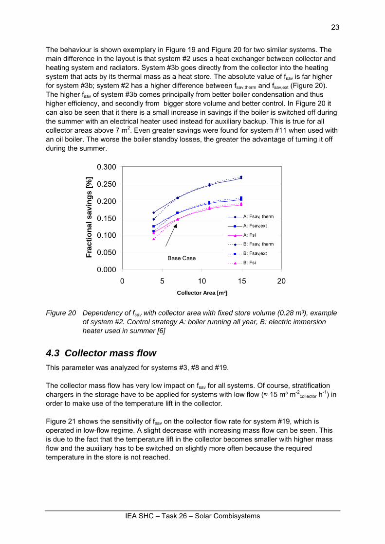
The behaviour is shown exemplary in Figure 19 and Figure 20 for two similar systems. The main difference in the layout is that system #2 uses a heat exchanger between collector and heating system and radiators. System #3b goes directly from the collector into the heating system that acts by its thermal mass as a heat store. The absolute value of fsav is far higher for system #3b; system #2 has a higher difference between fsav,therm and fsav,ext (Figure 20). The higher fsav of system #3b comes principally from better boiler condensation and thus higher efficiency, and secondly from bigger store volume and better control. In Figure 20 it can also be seen that it there is a small increase in savings if the boiler is switched off during the summer with an electrical heater used instead for auxiliary backup. This is true for all collector areas above 7 m2. Even greater savings were found for system #11 when used with an oil boiler. The worse the boiler standby losses, the greater the advantage of turning it off during the summer.
0.000
0.050
0.100
0.150
0.200
0.250
0.300
0 5 10 15 20Collector Area [m²]
Frac
tiona
l sav
ings
[%]
A: Fsav, therm
A: Fsav,ext
A: Fsi
B: Fsav, therm
B: Fsav,ext
B: FsiBase Case
Figure 20 Dependency of fsav with collector area with fixed store volume (0.28 m³), example of system #2. Control strategy A: boiler running all year, B: electric immersion heater used in summer [6]
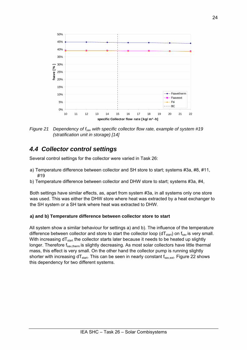
4.3 Collector mass flow This parameter was analyzed for systems #3, #8 and #19. The collector mass flow has very low impact on fsav for all systems. Of course, stratification chargers in the storage have to be applied for systems with low flow (≈ 15 m³ m-2
collector h-1) in order to make use of the temperature lift in the collector. Figure 21 shows the sensitivity of fsav on the collector flow rate for system #19, which is operated in low-flow regime. A slight decrease with increasing mass flow can be seen. This is due to the fact that the temperature lift in the collector becomes smaller with higher mass flow and the auxiliary has to be switched on slightly more often because the required temperature in the store is not reached.
IEA SHC – Task 26 – Solar Combisystems
24
0%
5%
10%
15%
20%
25%
30%
35%
40%
45%
50%
10 11 12 13 14 15 16 17 18 19 20 21 22
specific Collector flow rate [kg/m²-h]
fsav
e [%
]
FsavethermFsaveextFsiBC
Figure 21 Dependency of fsav with specific collector flow rate, example of system #19
(stratification unit in storage) [14]
4.4 Collector control settings Several control settings for the collector were varied in Task 26: a) Temperature difference between collector and SH store to start; systems #3a, #8, #11,
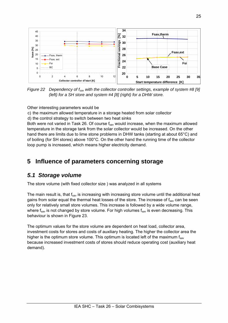
#19 b) Temperature difference between collector and DHW store to start; systems #3a, #4, Both settings have similar effects, as, apart from system #3a, in all systems only one store was used. This was either the DHW store where heat was extracted by a heat exchanger to the SH system or a SH tank where heat was extracted to DHW. a) and b) Temperature difference between collector store to start All system show a similar behaviour for settings a) and b). The influence of the temperature difference between collector and store to start the collector loop (dTstart) on fsav is very small. With increasing dTstart the collector starts later because it needs to be heated up slightly longer. Therefore fsav,therm is slightly decreasing. As most solar collectors have little thermal mass, this effect is very small. On the other hand the collector pump is running slightly shorter with increasing dTstart. This can be seen in nearly constant fsav,ext. Figure 22 shows this dependency for two different systems.
IEA SHC – Task 26 – Solar Combisystems
25
0
5
10
15
20
25
30
35
40
45
0 2 4 6 8 10 12
Collector controller dTstart [K]
fsav
e [%
]
Fsav, thermFsav, extFsiBC
20
22
24
26
28
30
32
34
0 5 10 15 20 25 30 35Start temperature difference [K]
Frac
tiona
l sav
ings
[%
] Fsav,therm
Fsav,ext
FsiBase Case
Figure 22 Dependency of fsav with the collector controller settings, example of system #8 [9] (left) for a SH store and system #4 [8] (right) for a DHW store.
Other interesting parameters would be c) the maximum allowed temperature in a storage heated from solar collector d) the control strategy to switch between two heat sinks Both were not varied in Task 26. Of course fsav would increase, when the maximum allowed temperature in the storage tank from the solar collector would be increased. On the other hand there are limits due to lime stone problems in DHW tanks (starting at about 65°C) and of boiling (for SH stores) above 100°C. On the other hand the running time of the collector loop pump is increased, which means higher electricity demand.
5 Influence of parameters concerning storage
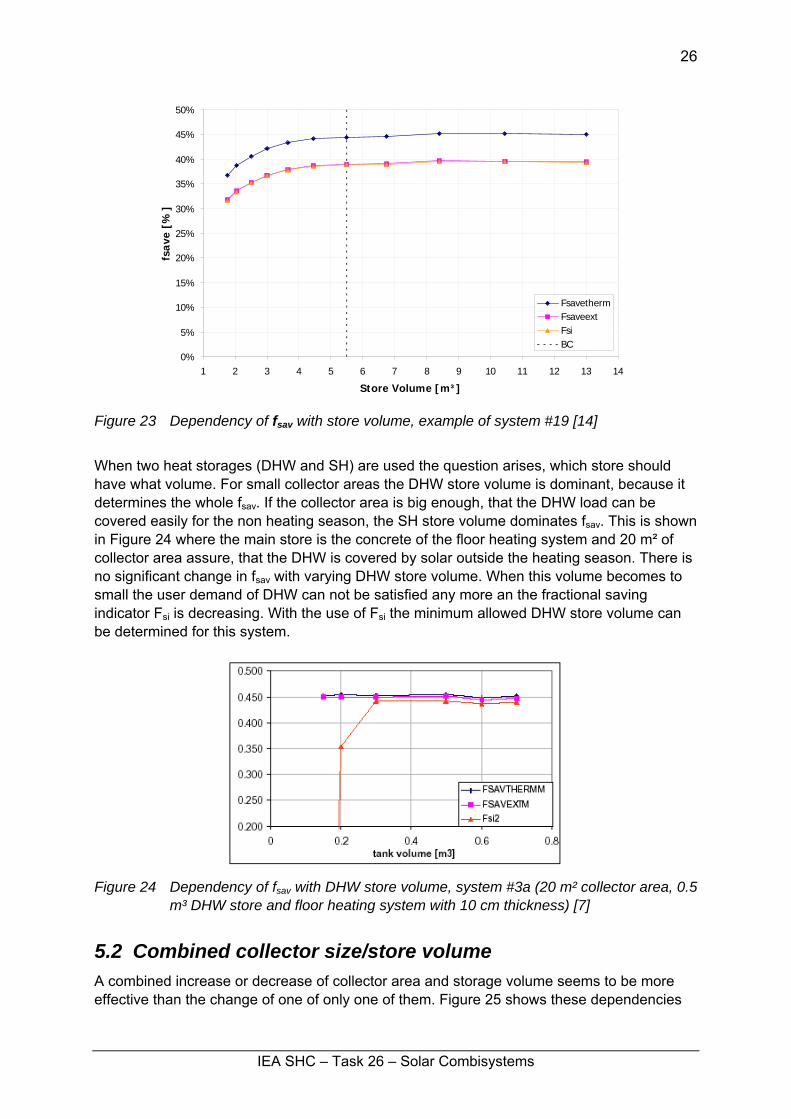
5.1 Storage volume The store volume (with fixed collector size ) was analyzed in all systems The main result is, that fsav is increasing with increasing store volume until the additional heat gains from solar equal the thermal heat losses of the store. The increase of fsav can be seen only for relatively small store volumes. This increase is followed by a wide volume range, where fsav is not changed by store volume. For high volumes fsav is even decreasing. This behaviour is shown in Figure 23. The optimum values for the store volume are dependent on heat load, collector area, investment costs for stores and costs of auxiliary heating. The higher the collector area the higher is the optimum store volume. This optimum is located left of the maximum fsav because increased investment costs of stores should reduce operating cost (auxiliary heat demand).
IEA SHC – Task 26 – Solar Combisystems
26
0%
5%
10%
15%
20%
25%
30%
35%
40%
45%
50%
1 2 3 4 5 6 7 8 9 10 11 12 13 14
Store Volume [m³]
fsav
e [%
]
FsavethermFsaveextFsiBC
Figure 23 Dependency of fsav with store volume, example of system #19 [14]
When two heat storages (DHW and SH) are used the question arises, which store should have what volume. For small collector areas the DHW store volume is dominant, because it determines the whole fsav. If the collector area is big enough, that the DHW load can be covered easily for the non heating season, the SH store volume dominates fsav. This is shown in Figure 24 where the main store is the concrete of the floor heating system and 20 m² of collector area assure, that the DHW is covered by solar outside the heating season. There is no significant change in fsav with varying DHW store volume. When this volume becomes to small the user demand of DHW can not be satisfied any more an the fractional saving indicator Fsi is decreasing. With the use of Fsi the minimum allowed DHW store volume can be determined for this system.
Figure 24 Dependency of fsav with DHW store volume, system #3a (20 m² collector area, 0.5
m³ DHW store and floor heating system with 10 cm thickness) [7]
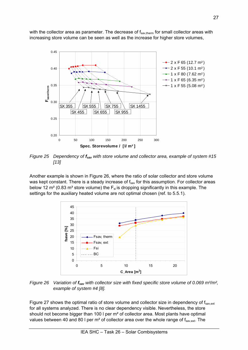
5.2 Combined collector size/store volume A combined increase or decrease of collector area and storage volume seems to be more effective than the change of one of only one of them. Figure 25 shows these dependencies
IEA SHC – Task 26 – Solar Combisystems
27
with the collector area as parameter. The decrease of fsav,therm for small collector areas with increasing store volume can be seen as well as the increase for higher store volumes,
0.20
0.25
0.30
0.35
0.40
0.45
0 50 100 150 200 250 300
Spec. Storevolume / [l/m²]
F sav
eth
erm
2 x F 65 (12.7 m²)2 x F 55 (10.1 m²)1 x F 80 (7.62 m²)1 x F 65 (6.35 m²)1 x F 55 (5.08 m²)SX 355SX 455SX 555SX 655SX 955SX 1455SX 755
SX 355SX 455
SX 555SX 655
SX 755SX 955
SX 1455
Figure 25 Dependency of fsav with store volume and collector area, example of system #15
[13]
Another example is shown in Figure 26, where the ratio of solar collector and store volume was kept constant. There is a steady increase of fsav for this assumption. For collector areas below 12 m² (0.83 m³ store volume) the Fsi is dropping significantly in this example. The settings for the auxiliary heated volume are not optimal chosen (ref. to 5.5.1).
0
510
1520
2530
3540
45
0 5 10 15 20
C_Area [m2]
fsav
e [%
]
Fsav, thermFsav, extFsiBC
Figure 26 Variation of fsav with collector size with fixed specific store volume of 0.069 m³/m², example of system #4 [8].
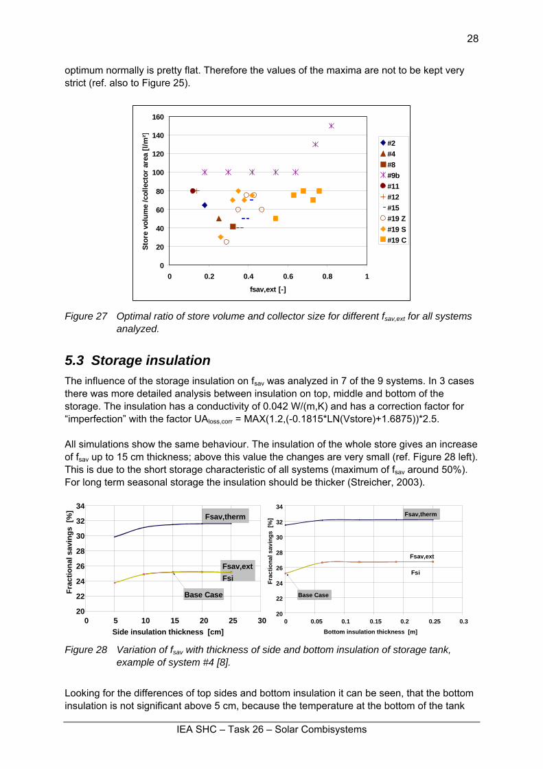
Figure 27 shows the optimal ratio of store volume and collector size in dependency of fsav,ext for all systems analyzed. There is no clear dependency visible. Nevertheless, the store should not become bigger than 100 l per m² of collector area. Most plants have optimal values between 40 and 80 l per m² of collector area over the whole range of fsav,ext. The
IEA SHC – Task 26 – Solar Combisystems
28
optimum normally is pretty flat. Therefore the values of the maxima are not to be kept very strict (ref. also to Figure 25).
0
20
40
60
80
100
120
140
160
0 0.2 0.4 0.6 0.8 1
fsav,ext [-]
Stor
e vo
lum
e /c
olle
ctor
are
a [l/
m²]
#2#4#8#9b#11#12#15#19 Z#19 S#19 C
Figure 27 Optimal ratio of store volume and collector size for different fsav,ext for all systems
analyzed.
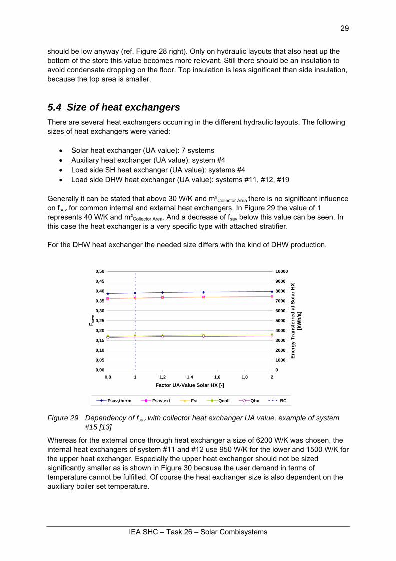
5.3 Storage insulation The influence of the storage insulation on fsav was analyzed in 7 of the 9 systems. In 3 cases there was more detailed analysis between insulation on top, middle and bottom of the storage. The insulation has a conductivity of 0.042 W/(m,K) and has a correction factor for “imperfection” with the factor UAloss,corr = MAX(1.2,(-0.1815*LN(Vstore)+1.6875))*2.5. All simulations show the same behaviour. The insulation of the whole store gives an increase of fsav up to 15 cm thickness; above this value the changes are very small (ref. Figure 28 left). This is due to the short storage characteristic of all systems (maximum of fsav around 50%). For long term seasonal storage the insulation should be thicker (Streicher, 2003).
20
22
24
26
28
30
32
34
0 5 10 15 20 25 30Side insulation thickness [cm]
Frac
tiona
l sav
ings
[%
]
Fsav,therm
Fsav,extFsi
Base Case
20
22
24
26
28
30
32
34
0 0.05 0.1 0.15 0.2 0.25 0.3Bottom insulation thickness [m]
Frac
tiona
l sav
ings
[%
] Fsav,therm
Fsav,ext
Fsi
Base Case
Figure 28 Variation of fsav with thickness of side and bottom insulation of storage tank,
example of system #4 [8].
Looking for the differences of top sides and bottom insulation it can be seen, that the bottom insulation is not significant above 5 cm, because the temperature at the bottom of the tank
IEA SHC – Task 26 – Solar Combisystems
29
should be low anyway (ref. Figure 28 right). Only on hydraulic layouts that also heat up the bottom of the store this value becomes more relevant. Still there should be an insulation to avoid condensate dropping on the floor. Top insulation is less significant than side insulation, because the top area is smaller.
5.4 Size of heat exchangers There are several heat exchangers occurring in the different hydraulic layouts. The following sizes of heat exchangers were varied:
• Solar heat exchanger (UA value): 7 systems • Auxiliary heat exchanger (UA value): system #4 • Load side SH heat exchanger (UA value): systems #4 • Load side DHW heat exchanger (UA value): systems #11, #12, #19
Generally it can be stated that above 30 W/K and m²Collector Area there is no significant influence on fsav for common internal and external heat exchangers. In Figure 29 the value of 1 represents 40 W/K and m²Collector Area. And a decrease of fsav below this value can be seen. In this case the heat exchanger is a very specific type with attached stratifier. For the DHW heat exchanger the needed size differs with the kind of DHW production.
0,00
0,05
0,10
0,15
0,20
0,25
0,30
0,35
0,40
0,45
0,50
0,8 1 1,2 1,4 1,6 1,8 2
Factor UA-Value Solar HX [-]
F sav
e
0
1000
2000
3000
4000
5000
6000
7000
8000
9000
10000
Ener
gy T
rans
ferr
ed a
t Sol
ar H
X [k
Wh/
a]
Fsav,therm Fsav,ext Fsi Qcoll Qhx BC
Figure 29 Dependency of fsav with collector heat exchanger UA value, example of system #15 [13]
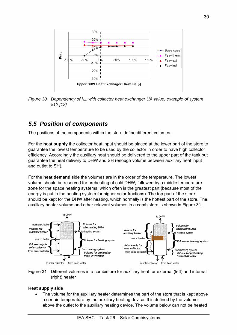
Whereas for the external once through heat exchanger a size of 6200 W/K was chosen, the internal heat exchangers of system #11 and #12 use 950 W/K for the lower and 1500 W/K for the upper heat exchanger. Especially the upper heat exchanger should not be sized significantly smaller as is shown in Figure 30 because the user demand in terms of temperature cannot be fulfilled. Of course the heat exchanger size is also dependent on the auxiliary boiler set temperature.
IEA SHC – Task 26 – Solar Combisystems
30
-30%
-20%
-10%
0%
10%
20%
30%
-100% -50% 0% 50% 100% 150%
Upper DHW Heat Exchnager UA-value [-]
Fsav
Base caseFsav,thermFsav,extFsav,ind
Figure 30 Dependency of fsav with collector heat exchanger UA value, example of system
#12 [12]
5.5 Position of components The positions of the components within the store define different volumes. For the heat supply the collector heat input should be placed at the lower part of the store to guarantee the lowest temperature to be used by the collector in order to have high collector efficiency. Accordingly the auxiliary heat should be delivered to the upper part of the tank but guarantee the heat delivery to DHW and SH (enough volume between auxiliary heat input and outlet to SH). For the heat demand side the volumes are in the order of the temperature. The lowest volume should be reserved for preheating of cold DHW, followed by a middle temperature zone for the space heating systems, which often is the greatest part (because most of the energy is put in the heating system for higher solar fractions). The top part of the store should be kept for the DHW after heating, which normally is the hottest part of the store. The auxiliary heater volume and other relevant volumes in a combistore is shown in Figure 31.
to heating system
from heating system
to DHW
from fresh water
from solar collector
to solar collector
Volume for heating system
Volume for afterheating DHW
Volume for preheating fresh DHW water
Volume only for solar collector
Volume for auxiliary heater }
}{{ }
from aux. boiler
to aux. boiler
to heating system
from heating system
to DHW
from fresh water
from solar collector
to solar collector
Volume for heating system
Volume for afterheating DHW
Volume for preheating fresh DHW water
Volume only for solar collector
Volume for auxiliary heater
Interal heater }}{
{ }
Figure 31 Different volumes in a combistore for auxiliary heat for external (left) and internal
(right) heater Heat supply side
• The volume for the auxiliary heater determines the part of the store that is kept above a certain temperature by the auxiliary heating device. It is defined by the volume above the outlet to the auxiliary heating device. The volume below can not be heated
IEA SHC – Task 26 – Solar Combisystems
31
by the auxiliary. The size of the volume is determined by the maximum heat demand that has to be guaranteed by the system, the required minimum running time and the heat capacity of the auxiliary heater.
• The volume only for the collector is unaffected by the auxiliary heater. It is defined as the volume between outlet to the collector (should be always at the bottom for external heat exchangers) or the lower end of the internal heat exchanger of the solar collector (which should be again as close as possible to the lower end of the boiler).
• If there remains a volume below the collector volume it can not be heated and is lost for the user (“dead volume”).
Heat demand side
• On the demand side the volume for the space heating system is between the inlet and outlet of the heating system.
• Below is the preheating zone of the fresh and cold DHW. • Above is the after heating zone of DHW, which is normally the hottest part of the
store • If there remains a volume above the highest outlet it can not be used for the demand
side and is “lost” volume.
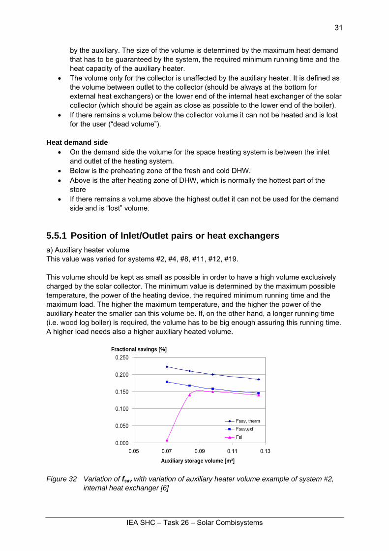
5.5.1 Position of Inlet/Outlet pairs or heat exchangers a) Auxiliary heater volume This value was varied for systems #2, #4, #8, #11, #12, #19. This volume should be kept as small as possible in order to have a high volume exclusively charged by the solar collector. The minimum value is determined by the maximum possible temperature, the power of the heating device, the required minimum running time and the maximum load. The higher the maximum temperature, and the higher the power of the auxiliary heater the smaller can this volume be. If, on the other hand, a longer running time (i.e. wood log boiler) is required, the volume has to be big enough assuring this running time. A higher load needs also a higher auxiliary heated volume.
0.000
0.050
0.100
0.150
0.200
0.250
0.05 0.07 0.09 0.11 0.13
Auxiliary storage volume [m³]
Fractional savings [%]
Fsav, thermFsav,extFsi
Figure 32 Variation of fsav with variation of auxiliary heater volume example of system #2,
internal heat exchanger [6]
IEA SHC – Task 26 – Solar Combisystems
32
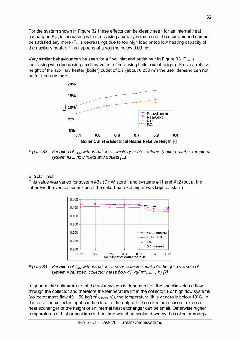
For the system shown in Figure 32 these effects can be clearly seen for an internal heat exchanger. Fsav is increasing with decreasing auxiliary volume until the user demand can not be satisfied any more (Fsi is decreasing) due to too high load or too low heating capacity of the auxiliary heater. This happens at a volume below 0.09 m³. Very similar behaviour can be seen for a flow inlet and outlet pair in Figure 33. Fsav is increasing with decreasing auxiliary volume (increasing boiler outlet height). Above a relative height of the auxiliary heater (boiler) outlet of 0.7 (about 0.230 m³) the user demand can not be fulfilled any more.
0%
5%
10%
15%
20%
0.4 0.5 0.6 0.7 0.8 0.9Boiler Outlet & Electrical Heater Relative Height [-]
f save
Fsav,thermFsav,extFsiBC
Figure 33 Variation of fsav with variation of auxiliary heater volume (boiler outlet) example of
system #11, flow inlets and outlets [11
b) Solar inlet This value was varied for system #3a (DHW store), and systems #11 and #12 (but at the latter two the vertical extension of the solar heat exchanger was kept constant)
Figure 34 Variation of fsav with variation of solar collector heat inlet height, example of
system #3a, spec. collector mass flow 40 kg/(m2collector,h) [7]
In general the optimum inlet of the solar system is dependent on the specific volume flow through the collector and therefore the temperature lift in the collector. For high flow systems (collector mass flow 40 – 50 kg/(m2
collector,h)), the temperature lift is generally below 10°C. In this case the collector input can be close to the output to the collector in case of external heat exchanger or the height of an internal heat exchanger can be small. Otherwise higher temperatures at higher positions in the store would be cooled down by the collector energy
IEA SHC – Task 26 – Solar Combisystems
33
input. This effect can be seen in Figure 34, where a light decrease with increasing inlet of solar can be seen. The higher decrease above 0.35 is probably an overlap with the auxiliary heat exchanger For low flow systems (collector mass flow 10 – 15 kg/(m2
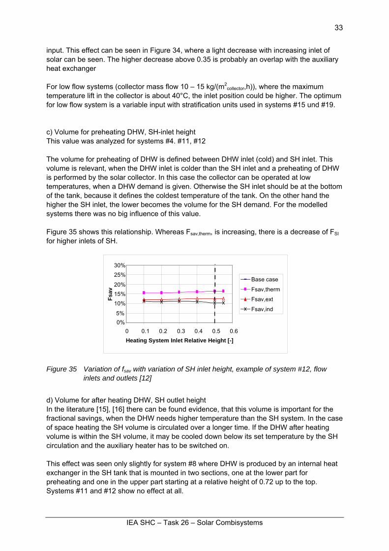
collector,h)), where the maximum temperature lift in the collector is about 40°C, the inlet position could be higher. The optimum for low flow system is a variable input with stratification units used in systems #15 und #19. c) Volume for preheating DHW, SH-inlet height This value was analyzed for systems #4. #11, #12 The volume for preheating of DHW is defined between DHW inlet (cold) and SH inlet. This volume is relevant, when the DHW inlet is colder than the SH inlet and a preheating of DHW is performed by the solar collector. In this case the collector can be operated at low temperatures, when a DHW demand is given. Otherwise the SH inlet should be at the bottom of the tank, because it defines the coldest temperature of the tank. On the other hand the higher the SH inlet, the lower becomes the volume for the SH demand. For the modelled systems there was no big influence of this value. Figure 35 shows this relationship. Whereas Fsav,therm, is increasing, there is a decrease of FSI for higher inlets of SH.
0%5%
10%15%20%
25%30%
0 0.1 0.2 0.3 0.4 0.5 0.6Heating System Inlet Relative Height [-]
Fsav
Base case
Fsav,therm
Fsav,ext
Fsav,ind
Figure 35 Variation of fsav with variation of SH inlet height, example of system #12, flow
inlets and outlets [12]
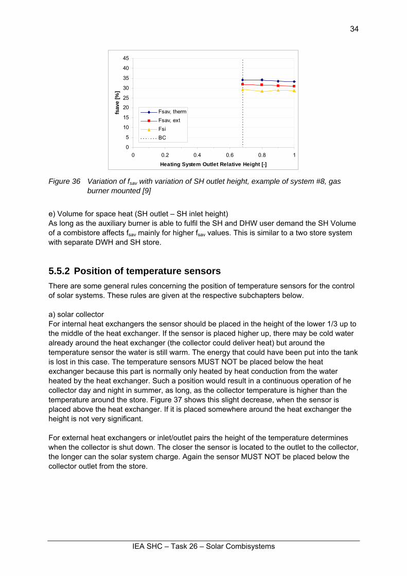
d) Volume for after heating DHW, SH outlet height In the literature [15], [16] there can be found evidence, that this volume is important for the fractional savings, when the DHW needs higher temperature than the SH system. In the case of space heating the SH volume is circulated over a longer time. If the DHW after heating volume is within the SH volume, it may be cooled down below its set temperature by the SH circulation and the auxiliary heater has to be switched on. This effect was seen only slightly for system #8 where DHW is produced by an internal heat exchanger in the SH tank that is mounted in two sections, one at the lower part for preheating and one in the upper part starting at a relative height of 0.72 up to the top. Systems #11 and #12 show no effect at all.
IEA SHC – Task 26 – Solar Combisystems
34
0
5
10
15
20
25
30
35
40
45
0 0.2 0.4 0.6 0.8 1
Heating System Outlet Relative Height [-]
fsav
e [%
]Fsav, thermFsav, extFsiBC
Figure 36 Variation of fsav with variation of SH outlet height, example of system #8, gas
burner mounted [9]
e) Volume for space heat (SH outlet – SH inlet height) As long as the auxiliary burner is able to fulfil the SH and DHW user demand the SH Volume of a combistore affects fsav mainly for higher fsav values. This is similar to a two store system with separate DWH and SH store.
5.5.2 Position of temperature sensors There are some general rules concerning the position of temperature sensors for the control of solar systems. These rules are given at the respective subchapters below. a) solar collector For internal heat exchangers the sensor should be placed in the height of the lower 1/3 up to the middle of the heat exchanger. If the sensor is placed higher up, there may be cold water already around the heat exchanger (the collector could deliver heat) but around the temperature sensor the water is still warm. The energy that could have been put into the tank is lost in this case. The temperature sensors MUST NOT be placed below the heat exchanger because this part is normally only heated by heat conduction from the water heated by the heat exchanger. Such a position would result in a continuous operation of he collector day and night in summer, as long, as the collector temperature is higher than the temperature around the store. Figure 37 shows this slight decrease, when the sensor is placed above the heat exchanger. If it is placed somewhere around the heat exchanger the height is not very significant. For external heat exchangers or inlet/outlet pairs the height of the temperature determines when the collector is shut down. The closer the sensor is located to the outlet to the collector, the longer can the solar system charge. Again the sensor MUST NOT be placed below the collector outlet from the store.
IEA SHC – Task 26 – Solar Combisystems
35
0%
5%
10%
15%
20%
0.0 0.1 0.2 0.3 0.4 0.5
Collector Controller Sensor Relative Height [-]
fsav
e
Fsav,thermFsav,extFsiBC
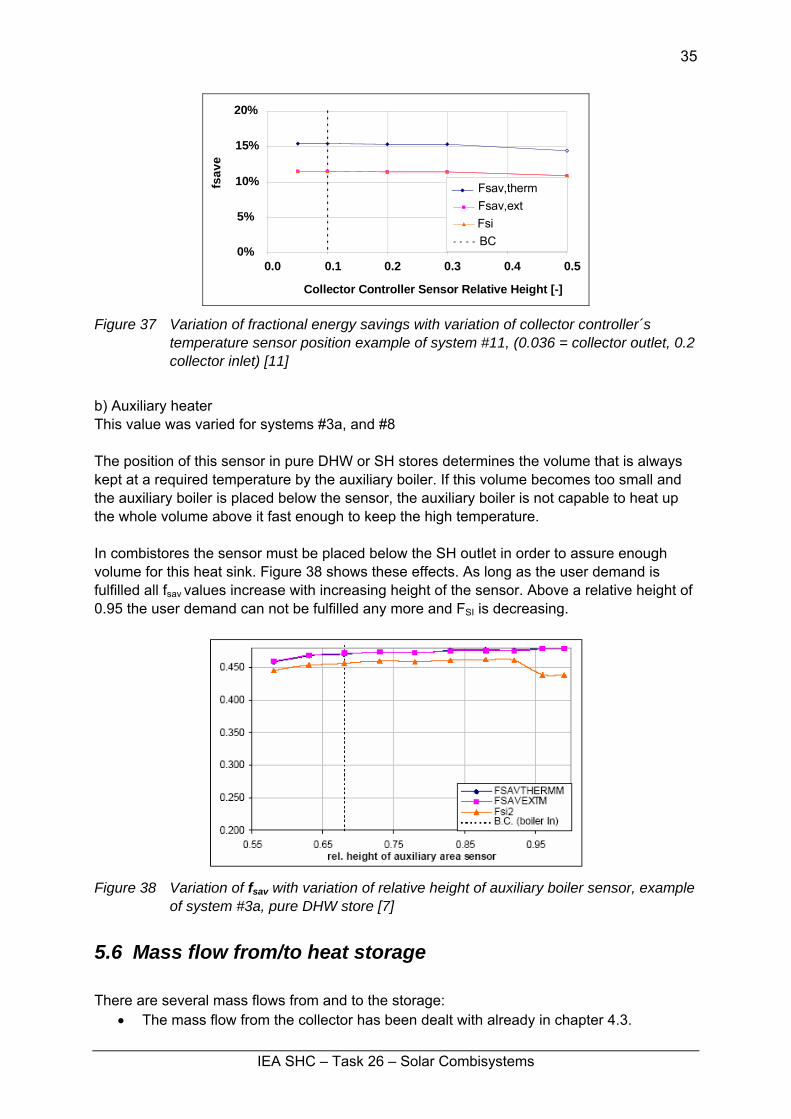
Figure 37 Variation of fractional energy savings with variation of collector controller´s temperature sensor position example of system #11, (0.036 = collector outlet, 0.2 collector inlet) [11]
b) Auxiliary heater This value was varied for systems #3a, and #8 The position of this sensor in pure DHW or SH stores determines the volume that is always kept at a required temperature by the auxiliary boiler. If this volume becomes too small and the auxiliary boiler is placed below the sensor, the auxiliary boiler is not capable to heat up the whole volume above it fast enough to keep the high temperature. In combistores the sensor must be placed below the SH outlet in order to assure enough volume for this heat sink. Figure 38 shows these effects. As long as the user demand is fulfilled all fsav values increase with increasing height of the sensor. Above a relative height of 0.95 the user demand can not be fulfilled any more and FSI is decreasing.
Figure 38 Variation of fsav with variation of relative height of auxiliary boiler sensor, example
of system #3a, pure DHW store [7]
5.6 Mass flow from/to heat storage There are several mass flows from and to the storage:
• The mass flow from the collector has been dealt with already in chapter 4.3.
IEA SHC – Task 26 – Solar Combisystems
36
• The mass flow from the auxiliary boiler is determined by the heating capacity and the temperature lift in the boiler. Normally either 10 – 20°C temperature lift for fixed capacity boilers or a boiler outlet temperature several °C above the actual needed temperature for capacity controlled burners are chosen.
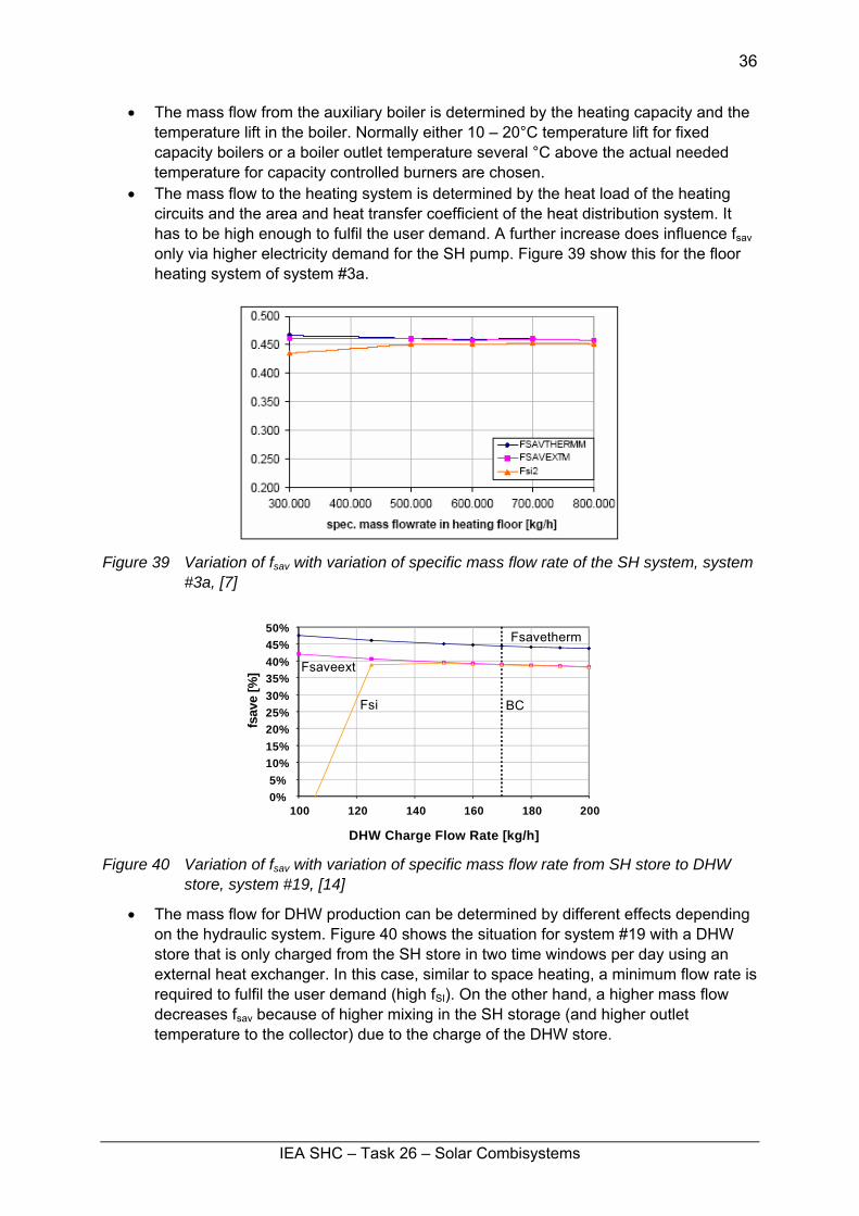
• The mass flow to the heating system is determined by the heat load of the heating circuits and the area and heat transfer coefficient of the heat distribution system. It has to be high enough to fulfil the user demand. A further increase does influence fsav only via higher electricity demand for the SH pump. Figure 39 show this for the floor heating system of system #3a.
Figure 39 Variation of fsav with variation of specific mass flow rate of the SH system, system
#3a, [7]
0%5%
10%15%20%25%30%35%40%45%50%
100 120 140 160 180 200
DHW Charge Flow Rate [kg/h]
fsav
e [%
]
Fsavetherm
Fsaveext
Fsi BC
Figure 40 Variation of fsav with variation of specific mass flow rate from SH store to DHW
store, system #19, [14]
• The mass flow for DHW production can be determined by different effects depending on the hydraulic system. Figure 40 shows the situation for system #19 with a DHW store that is only charged from the SH store in two time windows per day using an external heat exchanger. In this case, similar to space heating, a minimum flow rate is required to fulfil the user demand (high fSI). On the other hand, a higher mass flow decreases fsav because of higher mixing in the SH storage (and higher outlet temperature to the collector) due to the charge of the DHW store.
IEA SHC – Task 26 – Solar Combisystems
37
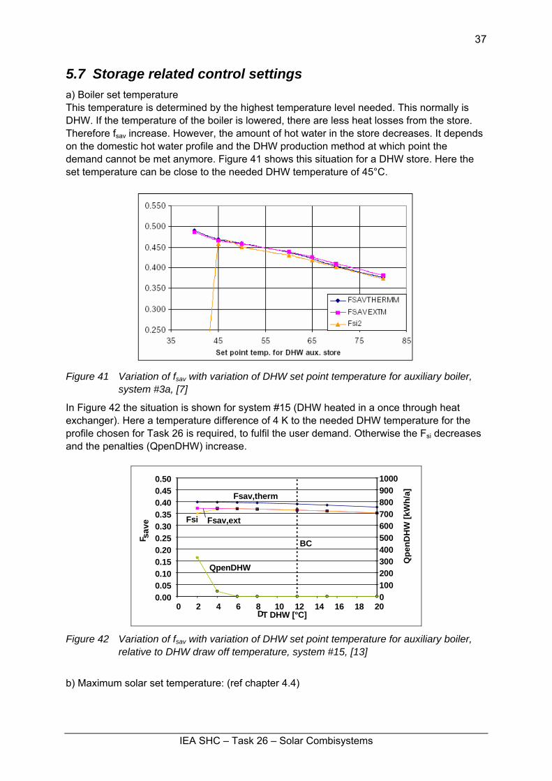
5.7 Storage related control settings a) Boiler set temperature This temperature is determined by the highest temperature level needed. This normally is DHW. If the temperature of the boiler is lowered, there are less heat losses from the store. Therefore fsav increase. However, the amount of hot water in the store decreases. It depends on the domestic hot water profile and the DHW production method at which point the demand cannot be met anymore. Figure 41 shows this situation for a DHW store. Here the set temperature can be close to the needed DHW temperature of 45°C.
Figure 41 Variation of fsav with variation of DHW set point temperature for auxiliary boiler,
system #3a, [7]
In Figure 42 the situation is shown for system #15 (DHW heated in a once through heat exchanger). Here a temperature difference of 4 K to the needed DHW temperature for the profile chosen for Task 26 is required, to fulfil the user demand. Otherwise the Fsi decreases and the penalties (QpenDHW) increase.
0.000.050.100.150.200.250.300.350.400.450.50
0 2 4 6 8 10 12 14 16 18 20DT DHW [°C]
F sav
e
01002003004005006007008009001000
Qpe
nDH
W [k
Wh/
a]Fsav,therm
Fsav,extFsi
QpenDHW
BC
Figure 42 Variation of fsav with variation of DHW set point temperature for auxiliary boiler,
relative to DHW draw off temperature, system #15, [13]
b) Maximum solar set temperature: (ref chapter 4.4)
IEA SHC – Task 26 – Solar Combisystems
38
6 Influence of boiler and SH system
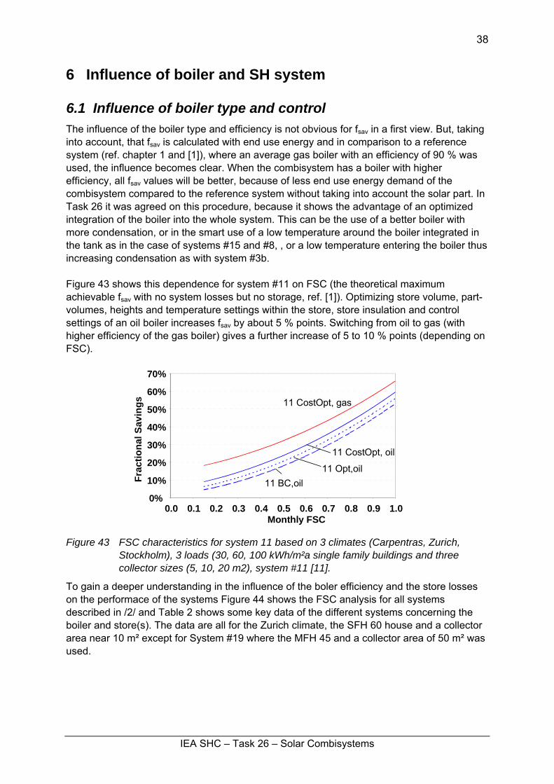
6.1 Influence of boiler type and control The influence of the boiler type and efficiency is not obvious for fsav in a first view. But, taking into account, that fsav is calculated with end use energy and in comparison to a reference system (ref. chapter 1 and [1]), where an average gas boiler with an efficiency of 90 % was used, the influence becomes clear. When the combisystem has a boiler with higher efficiency, all fsav values will be better, because of less end use energy demand of the combisystem compared to the reference system without taking into account the solar part. In Task 26 it was agreed on this procedure, because it shows the advantage of an optimized integration of the boiler into the whole system. This can be the use of a better boiler with more condensation, or in the smart use of a low temperature around the boiler integrated in the tank as in the case of systems #15 and #8, , or a low temperature entering the boiler thus increasing condensation as with system #3b. Figure 43 shows this dependence for system #11 on FSC (the theoretical maximum achievable fsav with no system losses but no storage, ref. [1]). Optimizing store volume, part-volumes, heights and temperature settings within the store, store insulation and control settings of an oil boiler increases fsav by about 5 % points. Switching from oil to gas (with higher efficiency of the gas boiler) gives a further increase of 5 to 10 % points (depending on FSC).
0%
10%
20%
30%
40%
50%
60%
70%
0.0 0.1 0.2 0.3 0.4 0.5 0.6 0.7 0.8 0.9 1.0Monthly FSC
Frac
tiona
l Sav
ings
11 BC,oil11 Opt,oil
11 CostOpt, oil
11 CostOpt, gas
Figure 43 FSC characteristics for system 11 based on 3 climates (Carpentras, Zurich,
Stockholm), 3 loads (30, 60, 100 kWh/m²a single family buildings and three collector sizes (5, 10, 20 m2), system #11 [11].
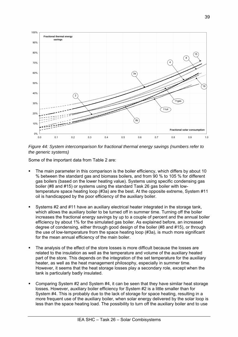
To gain a deeper understanding in the influence of the boler efficiency and the store losses on the performace of the systems Figure 44 shows the FSC analysis for all systems described in /2/ and Table 2 shows some key data of the different systems concerning the boiler and store(s). The data are all for the Zurich climate, the SFH 60 house and a collector area near 10 m² except for System #19 where the MFH 45 and a collector area of 50 m² was used.
IEA SHC – Task 26 – Solar Combisystems
39
0%
10%
20%
30%
40%
50%
60%
70%
80%
90%
100%
0.0 0.1 0.2 0.3 0.4 0.5 0.6 0.7 0.8 0.9 1.0
Fractional solar consumption
Fractional thermal energy savings
15
2
3a
8
11gas
11oil
9b
4
19
Figure 44: System intercomparison for fractional thermal energy savings (numbers refer to the generic systems)
Some of the important data from Table 2 are: The main parameter in this comparison is the boiler efficiency, which differs by about 10
% between the standard gas and biomass boilers, and from 90 % to 105 % for different gas boilers (based on the lower heating value). Systems using specific condensing gas boiler (#8 and #15) or systems using the standard Task 26 gas boiler with low-temperature space heating loop (#3a) are the best. At the opposite extreme, System #11 oil is handicapped by the poor efficiency of the auxiliary boiler.
Systems #2 and #11 have an auxiliary electrical heater integrated in the storage tank,
which allows the auxiliary boiler to be turned off in summer time. Turning off the boiler increases the fractional energy savings by up to a couple of percent and the annual boiler efficiency by about 1% for the simulated gas boiler. As explained before, an increased degree of condensing, either through good design of the boiler (#8 and #15), or through the use of low-temperature from the space heating loop (#3a), is much more significant for the mean annual efficiency of the main boiler.
The analysis of the effect of the store losses is more difficult because the losses are
related to the insulation as well as the temperature and volume of the auxiliary heated part of the store. This depends on the integration of the set temperature for the auxiliary heater, as well as the heat management philosophy, especially in summer time. However, it seems that the heat storage losses play a secondary role, except when the tank is particularly badly insulated.
Comparing System #2 and System #4, it can be seen that they have similar heat storage
losses. However, auxiliary boiler efficiency for System #2 is a little smaller than for System #4. This is probably due to the lack of storage for space heating, resulting in a more frequent use of the auxiliary boiler, when solar energy delivered by the solar loop is less than the space heating load. The possibility to turn off the auxiliary boiler and to use
IEA SHC – Task 26 – Solar Combisystems
40
the integrated electric heater in summer time, which should theoretically improve the annual efficiency, does not seem to be able to compensate for this effect.
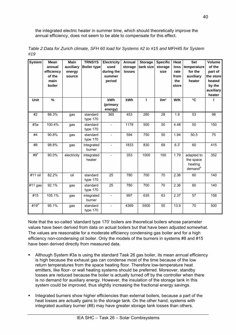
Table 2:Data for Zurich climate, SFH 60 load for Systems #2 to #15 and MFH45 for System #19
System Mean annual
efficiency of the main boiler
Main auxiliary energy source
TRNSYS Boiler type
Electricity used
during the summer period
Annual storage losses
Storage tank size
Specific storage
size
Heat loss rate from the
store
Set temperature
for the auxiliary heater
Volume of the part of
the store heated by the
auxiliary heater
Unit % kWh (primary energy)
kWh l l/m² W/K °C l
#2 88.3% gas standard type 170
365 453 280 28 1.9 53 98
#3a 100.4% gas standard type 170
- 1178 500 50 4.48 50 150
#4 90.8% gas standard type 170
- 594 750 50 1.94 50.5 75
#8 98.8% gas integrated burner
- 1833 830 69 6.3i 60 415
#9ii 90.0% electricity integrated heater
- 353 1000 100 1.79 adapted to the space heating
demandiii
352
#11 oil 82.2% oil standard type 170
25 780 700 70 2.36 60 140
#11 gas 92.1% gas standard type 170
25 780 700 70 2.36 60 140
#15 105.1% gas integrated burner
- 997 635 63 2.37 57 158
#19iv 95.1% gas
standard type 170
- 4369 5500 50 13.9 70 500
Note that the so-called ‘standard type 170’ boilers are theoretical boilers whose parameter values have been derived from data on actual boilers but that have been adjusted somewhat. The values are reasonable for a moderate efficiency condensing gas boiler and for a high efficiency non-condensing oil boiler. Only the models of the burners in systems #8 and #15 have been derived directly from measured data. Although System #3a is using the standard Task 26 gas boiler, its mean annual efficiency
is high because the exhaust gas can condense most of the time because of the low return temperatures from the space heating floor. Therefore low-temperature heat emitters, like floor- or wall heating systems should be preferred. Moreover, standby losses are reduced because the boiler is actually turned off by the controller when there is no demand for auxiliary energy. However, the insulation of the storage tank in this system could be improved, thus slightly increasing the fractional energy savings.
Integrated burners show higher efficiencies than external boilers, because a part of the
heat losses are actually gains to the storage tank. On the other hand, systems with integrated auxiliary burner (#8) may have greater storage tank losses than others.
IEA SHC – Task 26 – Solar Combisystems
41
Comparing Systems #15 and #3a, it can be seen that they have similar storage tank
losses. The difference between the two fsav curves is mainly related to the difference in the boiler efficiencies.
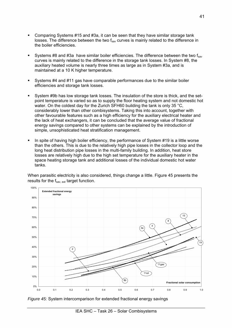
Systems #8 and #3a have similar boiler efficiencies. The difference between the two fsav
curves is mainly related to the difference in the storage tank losses. In System #8, the auxiliary heated volume is nearly three times as large as in System #3a, and is maintained at a 10 K higher temperature.
Systems #4 and #11 gas have comparable performances due to the similar boiler
efficiencies and storage tank losses. System #9b has low storage tank losses. The insulation of the store is thick, and the set-
point temperature is varied so as to supply the floor heating system and not domestic hot water. On the coldest day for the Zurich SFH60 building the tank is only 35 °C, considerably lower than other combisystems. Taking this into account, together with other favourable features such as a high efficiency for the auxiliary electrical heater and the lack of heat exchangers, it can be concluded that the average value of fractional energy savings compared to other systems can be explained by the introduction of simple, unsophisticated heat stratification management.
In spite of having high boiler efficiency, the performance of System #19 is a little worse
than the others. This is due to the relatively high pipe losses in the collector loop and the long heat distribution pipe losses in the multi-family building. In addition, heat store losses are relatively high due to the high set temperature for the auxiliary heater in the space heating storage tank and additional losses of the individual domestic hot water tanks.
When parasitic electricity is also considered, things change a little. Figure 45 presents the results for the fsav, ext target function.
0%
10%
20%
30%
40%
50%
60%
70%
80%
90%
100%
0.0 0.1 0.2 0.3 0.4 0.5 0.6 0.7 0.8 0.9 1.0
Fractional solar consumption
Extended fractional energy savings
15
2
3a
8
11gas
11oil
9b
4
19
Figure 45: System intercomparison for extended fractional energy savings
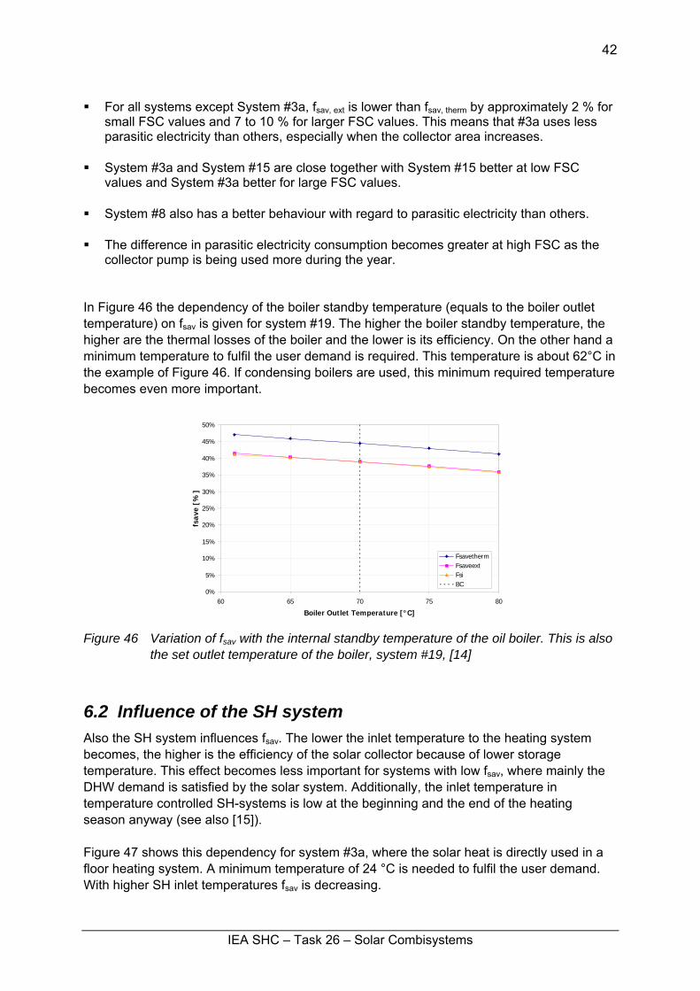
IEA SHC – Task 26 – Solar Combisystems
42
For all systems except System #3a, fsav, ext is lower than fsav, therm by approximately 2 % for
small FSC values and 7 to 10 % for larger FSC values. This means that #3a uses less parasitic electricity than others, especially when the collector area increases.
System #3a and System #15 are close together with System #15 better at low FSC
values and System #3a better for large FSC values. System #8 also has a better behaviour with regard to parasitic electricity than others.
The difference in parasitic electricity consumption becomes greater at high FSC as the
collector pump is being used more during the year. In Figure 46 the dependency of the boiler standby temperature (equals to the boiler outlet temperature) on fsav is given for system #19. The higher the boiler standby temperature, the higher are the thermal losses of the boiler and the lower is its efficiency. On the other hand a minimum temperature to fulfil the user demand is required. This temperature is about 62°C in the example of Figure 46. If condensing boilers are used, this minimum required temperature becomes even more important.
0%
5%
10%
15%
20%
25%
30%
35%
40%
45%
50%
60 65 70 75 80
Boiler Outlet Temperature [°C]
fsav
e [%
]
FsavethermFsaveextFsiBC
Figure 46 Variation of fsav with the internal standby temperature of the oil boiler. This is also
the set outlet temperature of the boiler, system #19, [14]
6.2 Influence of the SH system Also the SH system influences fsav. The lower the inlet temperature to the heating system becomes, the higher is the efficiency of the solar collector because of lower storage temperature. This effect becomes less important for systems with low fsav, where mainly the DHW demand is satisfied by the solar system. Additionally, the inlet temperature in temperature controlled SH-systems is low at the beginning and the end of the heating season anyway (see also [15]). Figure 47 shows this dependency for system #3a, where the solar heat is directly used in a floor heating system. A minimum temperature of 24 °C is needed to fulfil the user demand. With higher SH inlet temperatures fsav is decreasing.
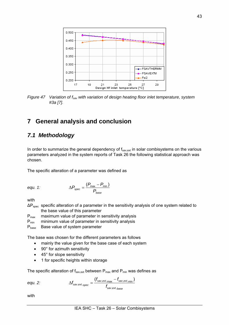
IEA SHC – Task 26 – Solar Combisystems
43
Figure 47 Variation of fsav with variation of design heating floor inlet temperature, system
#3a [7].
7 General analysis and conclusion
7.1 Methodology In order to summarize the general dependency of fsav,ext in solar combisystems on the various parameters analyzed in the system reports of Task 26 the following statistical approach was chosen. The specific alteration of a parameter was defined as
equ. 1: base
spec PPPP )( minmax −=Δ
with ΔPspec specific alteration of a parameter in the sensitivity analysis of one system related to
the base value of this parameter Pmax maximum value of parameter in sensitivity analysis Pmin minimum value of parameter in sensitivity analysis Pbase Base value of system parameter The base was chosen for the different parameters as follows
• mainly the value given for the base case of each system • 90° for azimuth sensitivity • 45° for slope sensitivity • 1 for specific heights within storage
The specific alteration of fsav,ext between Pmax and Pmin was defines as
equ. 2: baseextsav
extsavextsavspecextsav f
fff
,,
min,,max,,,,
)( −=Δ
with
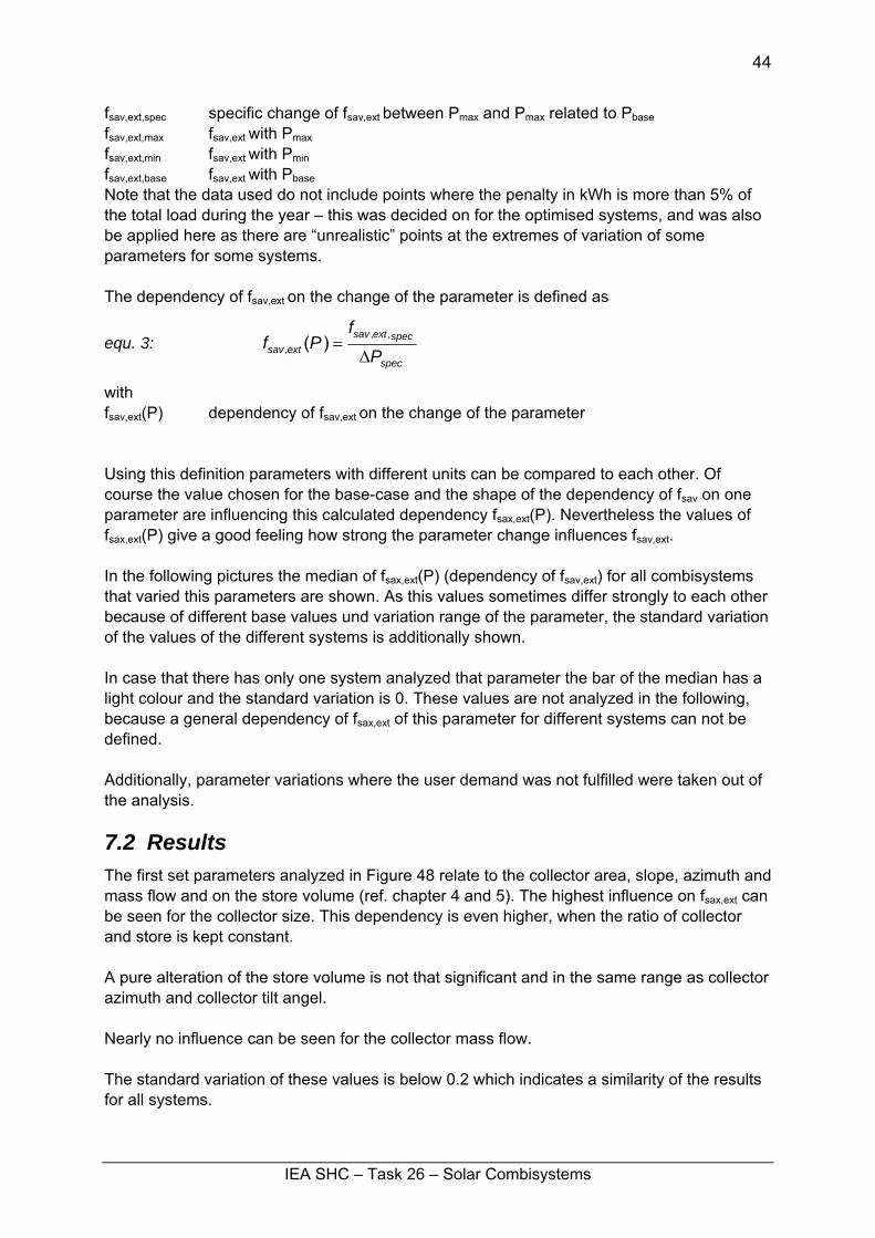
IEA SHC – Task 26 – Solar Combisystems
44
fsav,ext,spec specific change of fsav,ext between Pmax and Pmax related to Pbase fsav,ext,max fsav,ext with Pmax fsav,ext,min fsav,ext with Pmin
fsav,ext,base fsav,ext with Pbase
Note that the data used do not include points where the penalty in kWh is more than 5% of the total load during the year – this was decided on for the optimised systems, and was also be applied here as there are “unrealistic” points at the extremes of variation of some parameters for some systems. The dependency of fsav,ext on the change of the parameter is defined as
equ. 3: spec
specextsavextsav P
fPf
Δ=
,,, )(
with fsav,ext(P) dependency of fsav,ext on the change of the parameter Using this definition parameters with different units can be compared to each other. Of course the value chosen for the base-case and the shape of the dependency of fsav on one parameter are influencing this calculated dependency fsax,ext(P). Nevertheless the values of fsax,ext(P) give a good feeling how strong the parameter change influences fsav,ext. In the following pictures the median of fsax,ext(P) (dependency of fsav,ext) for all combisystems that varied this parameters are shown. As this values sometimes differ strongly to each other because of different base values und variation range of the parameter, the standard variation of the values of the different systems is additionally shown. In case that there has only one system analyzed that parameter the bar of the median has a light colour and the standard variation is 0. These values are not analyzed in the following, because a general dependency of fsax,ext of this parameter for different systems can not be defined. Additionally, parameter variations where the user demand was not fulfilled were taken out of the analysis.
7.2 Results The first set parameters analyzed in Figure 48 relate to the collector area, slope, azimuth and mass flow and on the store volume (ref. chapter 4 and 5). The highest influence on fsax,ext can be seen for the collector size. This dependency is even higher, when the ratio of collector and store is kept constant. A pure alteration of the store volume is not that significant and in the same range as collector azimuth and collector tilt angel. Nearly no influence can be seen for the collector mass flow. The standard variation of these values is below 0.2 which indicates a similarity of the results for all systems.
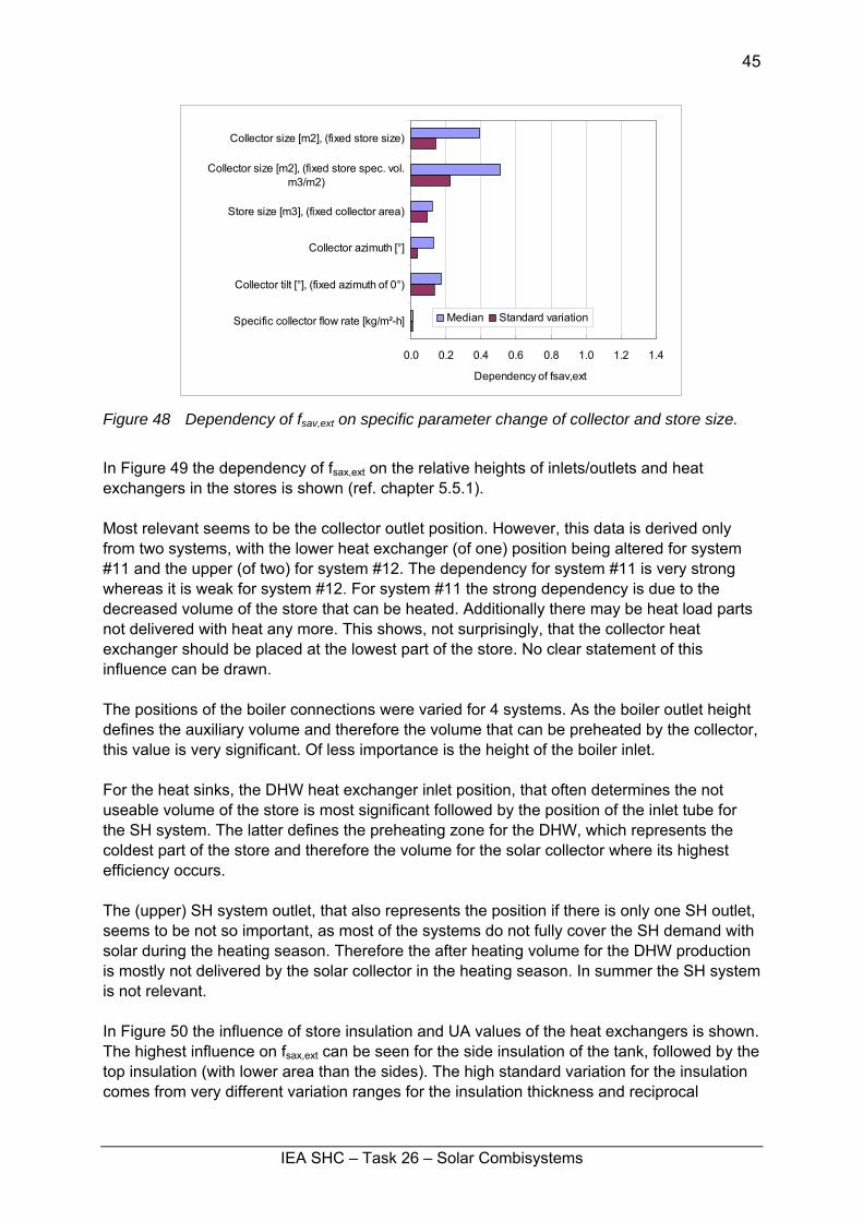
IEA SHC – Task 26 – Solar Combisystems
45
0.0 0.2 0.4 0.6 0.8 1.0 1.2 1.4
Collector size [m2], (fixed store size)
Collector size [m2], (fixed store spec. vol.m3/m2)
Store size [m3], (fixed collector area)
Collector azimuth [°]
Collector tilt [°], (fixed azimuth of 0°)
Specific collector flow rate [kg/m²-h]
Dependency of fsav,ext
Median Standard variation
Figure 48 Dependency of fsav,ext on specific parameter change of collector and store size.
In Figure 49 the dependency of fsax,ext on the relative heights of inlets/outlets and heat exchangers in the stores is shown (ref. chapter 5.5.1). Most relevant seems to be the collector outlet position. However, this data is derived only from two systems, with the lower heat exchanger (of one) position being altered for system #11 and the upper (of two) for system #12. The dependency for system #11 is very strong whereas it is weak for system #12. For system #11 the strong dependency is due to the decreased volume of the store that can be heated. Additionally there may be heat load parts not delivered with heat any more. This shows, not surprisingly, that the collector heat exchanger should be placed at the lowest part of the store. No clear statement of this influence can be drawn. The positions of the boiler connections were varied for 4 systems. As the boiler outlet height defines the auxiliary volume and therefore the volume that can be preheated by the collector, this value is very significant. Of less importance is the height of the boiler inlet. For the heat sinks, the DHW heat exchanger inlet position, that often determines the not useable volume of the store is most significant followed by the position of the inlet tube for the SH system. The latter defines the preheating zone for the DHW, which represents the coldest part of the store and therefore the volume for the solar collector where its highest efficiency occurs. The (upper) SH system outlet, that also represents the position if there is only one SH outlet, seems to be not so important, as most of the systems do not fully cover the SH demand with solar during the heating season. Therefore the after heating volume for the DHW production is mostly not delivered by the solar collector in the heating season. In summer the SH system is not relevant. In Figure 50 the influence of store insulation and UA values of the heat exchangers is shown. The highest influence on fsax,ext can be seen for the side insulation of the tank, followed by the top insulation (with lower area than the sides). The high standard variation for the insulation comes from very different variation ranges for the insulation thickness and reciprocal
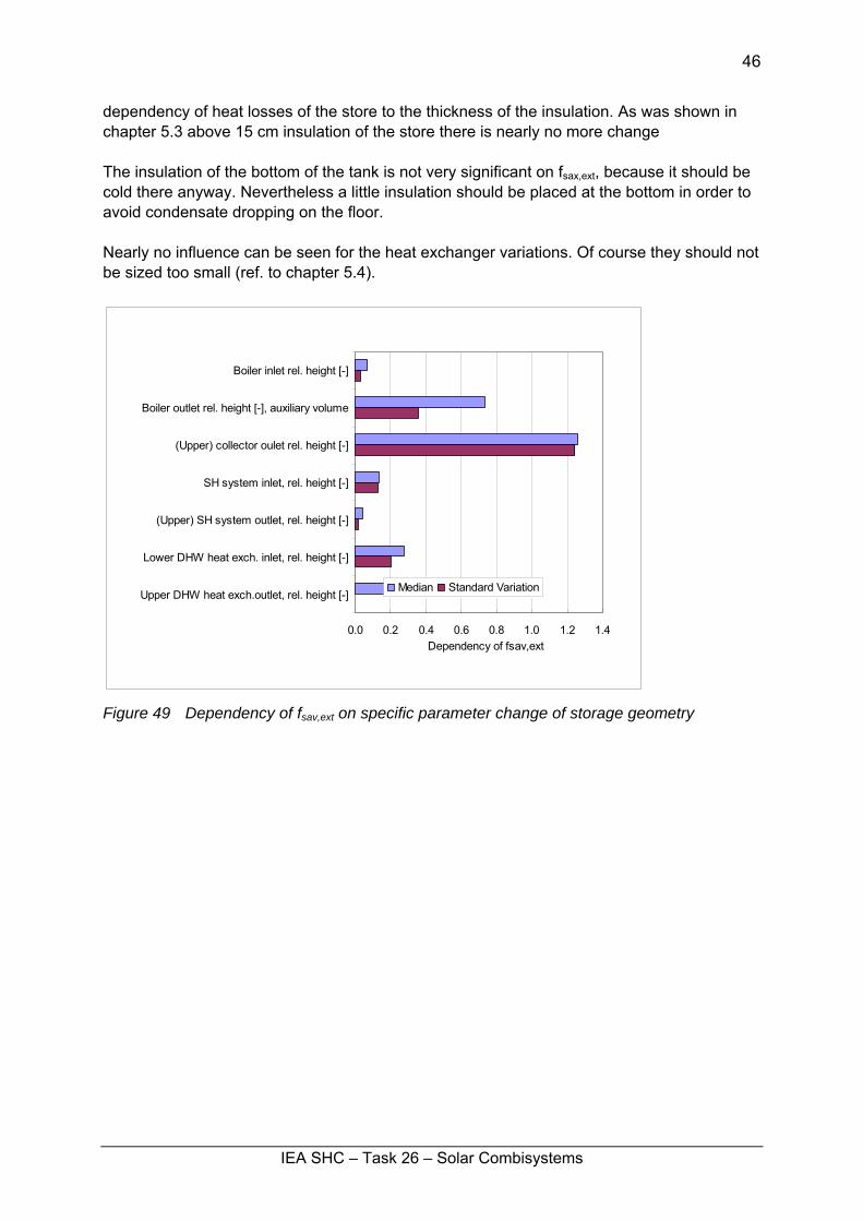
IEA SHC – Task 26 – Solar Combisystems
46
dependency of heat losses of the store to the thickness of the insulation. As was shown in chapter 5.3 above 15 cm insulation of the store there is nearly no more change The insulation of the bottom of the tank is not very significant on fsax,ext, because it should be cold there anyway. Nevertheless a little insulation should be placed at the bottom in order to avoid condensate dropping on the floor. Nearly no influence can be seen for the heat exchanger variations. Of course they should not be sized too small (ref. to chapter 5.4).
0.0 0.2 0.4 0.6 0.8 1.0 1.2 1.4
Boiler inlet rel. height [-]
Boiler outlet rel. height [-], auxiliary volume
(Upper) collector oulet rel. height [-]
SH system inlet, rel. height [-]
(Upper) SH system outlet, rel. height [-]
Lower DHW heat exch. inlet, rel. height [-]
Upper DHW heat exch.outlet, rel. height [-]
Dependency of fsav,ext
Median Standard Variation
Figure 49 Dependency of fsav,ext on specific parameter change of storage geometry
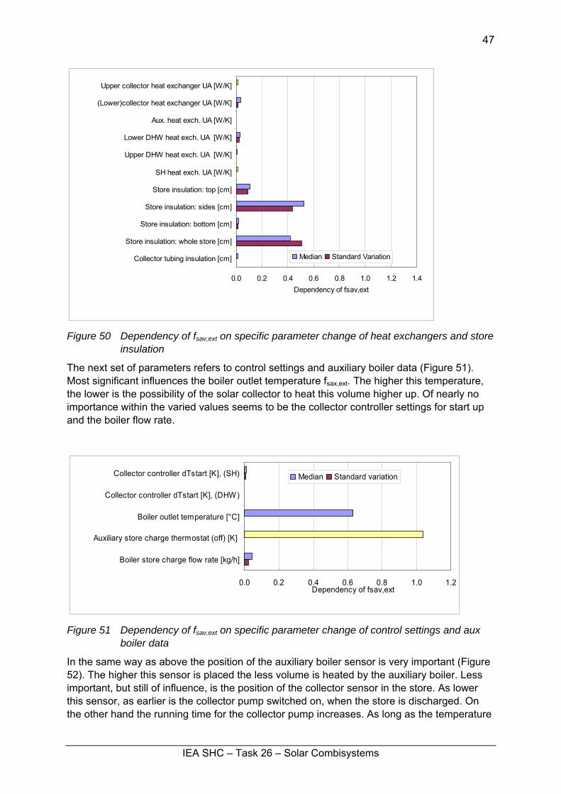
IEA SHC – Task 26 – Solar Combisystems
47
0.0 0.2 0.4 0.6 0.8 1.0 1.2 1.4
Upper collector heat exchanger UA [W/K]
(Lower)collector heat exchanger UA [W/K]
Aux. heat exch. UA [W/K]
Lower DHW heat exch. UA [W/K]
Upper DHW heat exch. UA [W/K]
SH heat exch. UA [W/K]
Store insulation: top [cm]
Store insulation: sides [cm]
Store insulation: bottom [cm]
Store insulation: whole store [cm]
Collector tubing insulation [cm]
Dependency of fsav,ext
Median Standard Variation
Figure 50 Dependency of fsav,ext on specific parameter change of heat exchangers and store
insulation
The next set of parameters refers to control settings and auxiliary boiler data (Figure 51). Most significant influences the boiler outlet temperature fsax,ext. The higher this temperature, the lower is the possibility of the solar collector to heat this volume higher up. Of nearly no importance within the varied values seems to be the collector controller settings for start up and the boiler flow rate.
0.0 0.2 0.4 0.6 0.8 1.0 1.2
Collector controller dTstart [K], (SH)
Collector controller dTstart [K], (DHW)
Boiler outlet temperature [°C]
Auxiliary store charge thermostat (off) [K]
Boiler store charge flow rate [kg/h]
Dependency of fsav,ext
Median Standard variation
Figure 51 Dependency of fsav,ext on specific parameter change of control settings and aux
boiler data
In the same way as above the position of the auxiliary boiler sensor is very important (Figure 52). The higher this sensor is placed the less volume is heated by the auxiliary boiler. Less important, but still of influence, is the position of the collector sensor in the store. As lower this sensor, as earlier is the collector pump switched on, when the store is discharged. On the other hand the running time for the collector pump increases. As long as the temperature
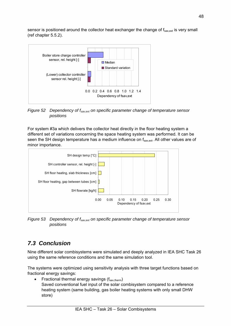
IEA SHC – Task 26 – Solar Combisystems
48
sensor is positioned around the collector heat exchanger the change of fsax,ext is very small (ref chapter 5.5.2).
0.0 0.2 0.4 0.6 0.8 1.0 1.2 1.4
Boiler store charge controllersensor, rel. height [-]
(Lower) collector controllersensor rel. height [-]
Dependency of fsav,ext
Median
Standard variation
Figure 52 Dependency of fsav,ext on specific parameter change of temperature sensor
positions
For system #3a which delivers the collector heat directly in the floor heating system a different set of variations concerning the space heating system was performed. It can be seen the SH design temperature has a medium influence on fsax,ext. All other values are of minor importance.
0.00 0.05 0.10 0.15 0.20 0.25 0.30
SH design temp [°C]
SH controller sensor, rel. height [-]
SH floor heating, slab thickness [cm]
SH floor heating, gap between tubes [cm]
SH flowrate [kg/h]
Dependency of fsav,ext
Figure 53 Dependency of fsav,ext on specific parameter change of temperature sensor
positions
7.3 Conclusion Nine different solar combisystems were simulated and deeply analyzed in IEA SHC Task 26 using the same reference conditions and the same simulation tool. The systems were optimized using sensitivity analysis with three target functions based on fractional energy savings:
• Fractional thermal energy savings (fsav,therm) Saved conventional fuel input of the solar combisystem compared to a reference heating system (same building, gas boiler heating systems with only small DHW store)
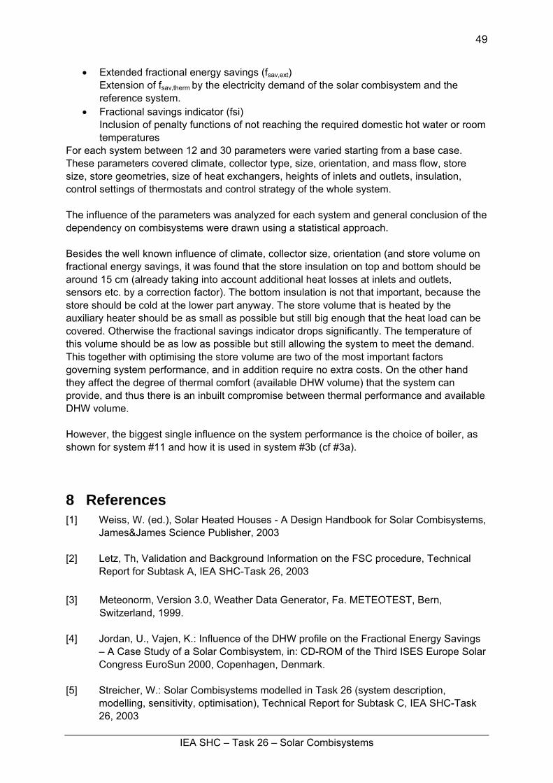
IEA SHC – Task 26 – Solar Combisystems
49
• Extended fractional energy savings (fsav,ext) Extension of fsav,therm by the electricity demand of the solar combisystem and the reference system.
• Fractional savings indicator (fsi) Inclusion of penalty functions of not reaching the required domestic hot water or room temperatures
For each system between 12 and 30 parameters were varied starting from a base case. These parameters covered climate, collector type, size, orientation, and mass flow, store size, store geometries, size of heat exchangers, heights of inlets and outlets, insulation, control settings of thermostats and control strategy of the whole system. The influence of the parameters was analyzed for each system and general conclusion of the dependency on combisystems were drawn using a statistical approach. Besides the well known influence of climate, collector size, orientation (and store volume on fractional energy savings, it was found that the store insulation on top and bottom should be around 15 cm (already taking into account additional heat losses at inlets and outlets, sensors etc. by a correction factor). The bottom insulation is not that important, because the store should be cold at the lower part anyway. The store volume that is heated by the auxiliary heater should be as small as possible but still big enough that the heat load can be covered. Otherwise the fractional savings indicator drops significantly. The temperature of this volume should be as low as possible but still allowing the system to meet the demand. This together with optimising the store volume are two of the most important factors governing system performance, and in addition require no extra costs. On the other hand they affect the degree of thermal comfort (available DHW volume) that the system can provide, and thus there is an inbuilt compromise between thermal performance and available DHW volume. However, the biggest single influence on the system performance is the choice of boiler, as shown for system #11 and how it is used in system #3b (cf #3a).
8 References [1] Weiss, W. (ed.), Solar Heated Houses - A Design Handbook for Solar Combisystems,
James&James Science Publisher, 2003 [2] Letz, Th, Validation and Background Information on the FSC procedure, Technical
Report for Subtask A, IEA SHC-Task 26, 2003 [3] Meteonorm, Version 3.0, Weather Data Generator, Fa. METEOTEST, Bern,
Switzerland, 1999. [4] Jordan, U., Vajen, K.: Influence of the DHW profile on the Fractional Energy Savings
– A Case Study of a Solar Combisystem, in: CD-ROM of the Third ISES Europe Solar Congress EuroSun 2000, Copenhagen, Denmark.
[5] Streicher, W.: Solar Combisystems modelled in Task 26 (system description,
modelling, sensitivity, optimisation), Technical Report for Subtask C, IEA SHC-Task 26, 2003
IEA SHC – Task 26 – Solar Combisystems
50
[6] Ellehauge, K.: Generic System #2: A Solar Combisystem based on a Heat Exchanger
between the Collector Loop and Space-Heating Loop, Technical Report for Subtask C, IEA SHC-Task 26, Appendix 1 to [5], 2003
[7] Cheze, D, Papillon, P.: Generic System #3a: Advanced Direct Solar Floor, Technical
Report for Subtask C, IEA SHC-Task 26, Appendix 2 to [5], 2003 [8] Shah, L.S.: Generic System #4: DHW Tank as Space-Heating Storage Device,
Technical Report for Subtask C, IEA SHC-Task 26, Appendix 3 to [5], 2003 [9] Bony, J., Pittet, J.: Generic System #8: Space Heating Store with Double Load-Side
Heat Exchanger for DHW, Technical Report for Subtask C, IEA SHC-Task 26, Appendix 4 to [5], 2003
[10] Peter, M.: Generic System #9b: Space Heating Store with Immersed DHW tank and
External DHW store with Auxiliary, Technical Report for Subtask C, IEA SHC-Task 26, Appendix 5 to [5], 2003
[11] Bales, C.: Generic System #11: Space Heating Store with DHW Load Side Heat
Exchanger(s) and External Auxiliary Boiler, Technical Report for Subtask C, IEA SHC-Task 26, Appendix 6 to [5], 2003
[12] Bales, C.: Generic System #12: Space Heating Store with DHW Load Side Heat
Exchanger(s) and External Auxiliary Boiler (Advanced Version), Technical Report for Subtask C, IEA SHC-Task 26, Appendix 7 to [5], 2003
[13] Jaehnig, D.: Generic System #15: Two stratifiers in a Space Heating Storage Tank
with an External Load-Side Heat Exchanger for DHW, Technical Report for Subtask C, IEA SHC-Task 26, Appendix 8 to [5], 2003
[14] Heimrath, R.: Generic System #19: Centralized Heat Production, Distributed Heat
Load, Technical Report for Subtask C, IEA SHC-Task 26, Appendix 9 to [5], 2003 [15] Streicher, W.: Sonnenenergienutzung, Lecture book, Graz University of Technology,
http://wt.tu-graz.ac.at, 2003 [16] Streicher, W. (1996), Analyse und Optimierung einer teilsolaren Heizungsanlage, 6.
Symposium Thermische Solarenergie, Kloster Banz, D-96231 Staffelstein. Hrsg.: OTTI-Technologie-Kolleg, Wernerwerkstr. 4, D-93049 Regensburg, S.285 289.
i Integrated burner losses taken into account ii Values are given for the space heating storage tank. Auxiliary energy for domestic hot water is brought in a separate small tank (80 l), with a heat loss rate of 1 W/K and a set-point temperature of 47.5 °C iii 35 °C for the coldest day for the SFH60 building in the Zurich climate iv Values are given for the space heating storage tank. Domestic hot water is heated in 5 separate small tanks (250 l), with a heat loss rate of 2.8 W/K and a set-point temperature of 60 °C. The additional annual storage losses are 2864 kWh for these 5 tanks.