HAL Id: hal-01061680https://hal.archives-ouvertes.fr/hal-01061680

Submitted on 8 Sep 2014

HAL is a multi-disciplinary open accessarchive for the deposit and dissemination of sci-entific research documents, whether they are pub-lished or not. The documents may come fromteaching and research institutions in France orabroad, or from public or private research centers.

L’archive ouverte pluridisciplinaire HAL, estdestinée au dépôt et à la diffusion de documentsscientifiques de niveau recherche, publiés ou non,émanant des établissements d’enseignement et derecherche français ou étrangers, des laboratoirespublics ou privés.

Analysis of the environmental magnetic noise rejectionby using two simple magnetoelectric sensors

Ying Shen, Junqi Gao, Liangguo Shen, D. Gray, Jiefang Li, Peter Finkel,Dwight Viehland, Xin Zhuang, Sebastien Saez, Christophe Dolabdjian

To cite this version:Ying Shen, Junqi Gao, Liangguo Shen, D. Gray, Jiefang Li, et al.. Analysis of the environmentalmagnetic noise rejection by using two simple magnetoelectric sensors. Sensors and Actuators A:Physical , Elsevier, 2011, 171, pp.63-68. �hal-01061680�

Accepted Manuscript

Title: Analysis of the environmental magnetic noise rejectionby using two simple magnetoelectric sensors

Authors: Y. Shen, J. Gao, L. Shen, D. Gray, J. Li, P. Finkel, D.Viehland, X. Zhuang, S. Saez, C. Dolabdjian

PII: S0924-4247(11)00478-XDOI: doi:10.1016/j.sna.2011.08.013Reference: SNA 7474

To appear in: Sensors and Actuators A

Received date: 9-2-2011Revised date: 19-7-2011Accepted date: 14-8-2011

Please cite this article as: Y. Shen, J. Gao, L. Shen, D. Gray, J. Li, P. Finkel, D.Viehland, X. Zhuang, S. Saez, C. Dolabdjian, Analysis of the environmental magneticnoise rejection by using two simple magnetoelectric sensors, Sensors and Actuators: APhysical (2010), doi:10.1016/j.sna.2011.08.013

This is a PDF file of an unedited manuscript that has been accepted for publication.As a service to our customers we are providing this early version of the manuscript.The manuscript will undergo copyediting, typesetting, and review of the resulting proofbefore it is published in its final form. Please note that during the production processerrors may be discovered which could affect the content, and all legal disclaimers thatapply to the journal pertain.

Page 1 of 18

Accep

ted

Man

uscr

ipt

Analysis of the environmental magnetic noise rejection by using two simple magnetoelectric sensors Y. Shen1, J. Gao1, L. Shen1, D. Gray1, J. Li1, P. Finkel2, D. Viehland1, X. Zhuang3, S. Saez3 and C. Dolabdjian3 1Department of Materials Science and Engineering, Virginia Tech, Blacksburg, Virginia 24061, USA 2Naval Undersea Warfare Center, Newport, Rhode island 02840, USA 3Groupe de Recherche en Informatique, Image, Automatique et Instrumentation de Caen (GREYC), CNRS UMR 6072–ENSICAEN and the University of Caen, France 14050 Caen Cedex We have evaluated the performance of a classical differential technique to reject magnetic or, in a lesser extent, the vibrational coherent noise sources sensed by two identical magnetoelectric (ME) laminated sensors with the help of a data logger. The signals of two ME sensors were directly subtracted given highly homogeneous external noise. Through a signal processing technique, the intrinsic noise of the ME sensor systems was obtained to be 20 pT/√Hz with a rejection factor of the external homogeneous noise sources of 20. The latter is mainly limited, as theoretical described, by the incoherent noise and discrepancy between the sensors. To demonstrate the efficiency of this technique by using ME sensors, internal noise tests were also performed in a magnetic shielding chamber for individual ME sensor and shown to be close to that of the sensors in an open environment. Introduction There is a large market for compact and effective man-portable magnetic sensor systems [1, 2]. Most existing magnetic sensor types have critical drawbacks. Superconducting quantum interference devices (SQUID) require extreme low operational temperatures to reach high sensitivity [3, 4]. Fluxgate sensors face detection limitations due to magnetic hysteresis, zero-field offset voltages, and demagnetization factors [5-7]. Giant magnetoresistive (GMR) or Giant magnetoimpedance (GMI) sensors have intrinsically a poorer linearity than ME and require mA DC bias current. All required feedback field loop to improve their performances in term of dynamic range. Laminate composite magnetoelectric (ME) sensors do not face the same limitations as other sensor types. Metglas/ Pb(Zr,Ti)O3 (PZT) multi-push-pull mode laminates are very low-power and room temperature magnetic sensor devices [8]. These ME laminate sensors consist of a magnetostrictive layer that is elastically coupled to a piezoelectric layer. A strain induced on the magnetostrictive layer by an incident magnetic field or on the piezoelectric layer by an incident vibration then produces a charge in the piezoelectric one [9, 10]. Values of the ME voltage coefficient have been found to be as highest αME = 20 V/(cm-Oe) in tri-layer Metglas/PZT/Metglas heterostructures and a lowest detectable magnetic field (f = 1 Hz) of 1 nT [10, 11]. Recently, by optimization of the metglas layer thickness, ME sensor has been improved to achieve the best possible sensitivity of 0.6 nT [12]. In most applications, magnetic sensors must be operated in an open (i.e., magnetically unshielded) environment. Such environments are contaminated by environmental noise, which can raise the equivalent magnetic noise floor of any magnetic sensor dramatically. In other words, for practical use ME magnetic sensor is fundamentally challenged by the inability to distinguish minute target signals from external noises which have several orders of higher amplitudes than former. As environmental shielding of magnetic sensors is impractical in numerous applications, using two (or more) magnetic sensors in a differential mode configuration is expected to reject/reduce environmental magnetic noise. Recent studies have indicated that such configurations are capable of rejecting common noise sources that are coherently shared between two sensors spatially separated by a baseline or sensor arrays [13, 14]. However, there has been no experimental report so far on the differential gradiometry measurement on ME sensor to reject environmental noises that are are coherently shared between two sensors separated by a baseline. Here, we focus on the analysis of the magnetic detection potentiality to optimize ME differentiator more sensitive for device applicatins.We evaluate the efficiency of coherent noise rejection and analyze the capacity of intrinsic noise

Page 2 of 18

Accep

ted

Man

uscr

ipt

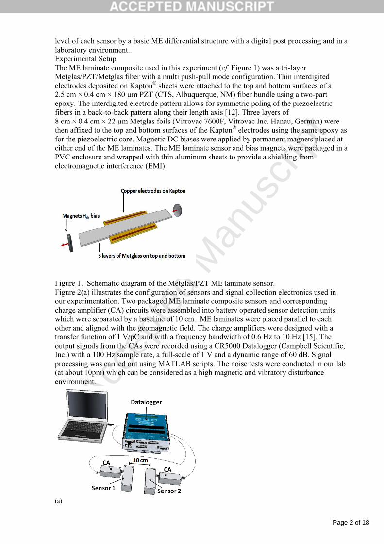
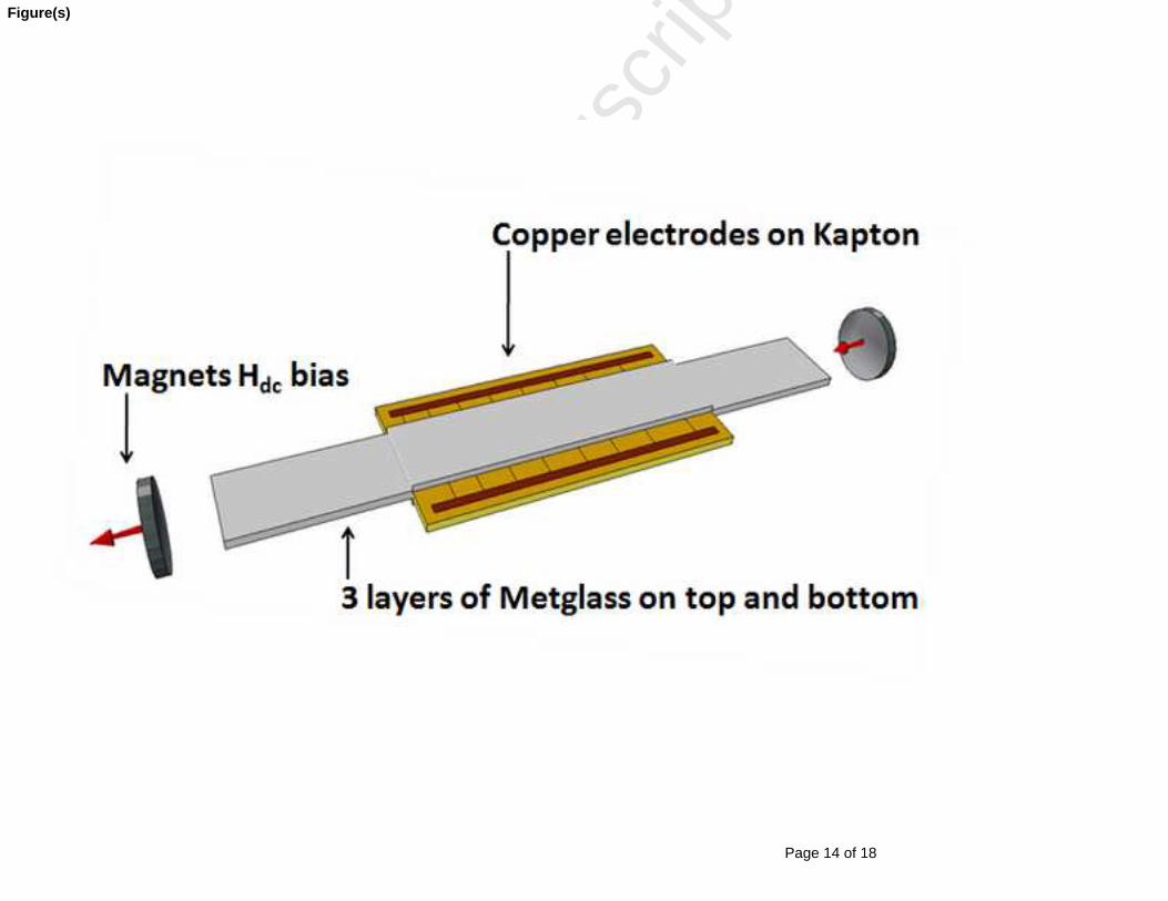
level of each sensor by a basic ME differential structure with a digital post processing and in a laboratory environment.. Experimental Setup The ME laminate composite used in this experiment (cf. Figure 1) was a tri-layer Metglas/PZT/Metglas fiber with a multi push-pull mode configuration. Thin interdigited electrodes deposited on Kapton® sheets were attached to the top and bottom surfaces of a 2.5 cm × 0.4 cm × 180 µm PZT (CTS, Albuquerque, NM) fiber bundle using a two-part epoxy. The interdigited electrode pattern allows for symmetric poling of the piezoelectric fibers in a back-to-back pattern along their length axis [12]. Three layers of 8 cm × 0.4 cm × 22 µm Metglas foils (Vitrovac 7600F, Vitrovac Inc. Hanau, German) were then affixed to the top and bottom surfaces of the Kapton® electrodes using the same epoxy as for the piezoelectric core. Magnetic DC biases were applied by permanent magnets placed at either end of the ME laminates. The ME laminate sensor and bias magnets were packaged in a PVC enclosure and wrapped with thin aluminum sheets to provide a shielding from electromagnetic interference (EMI).

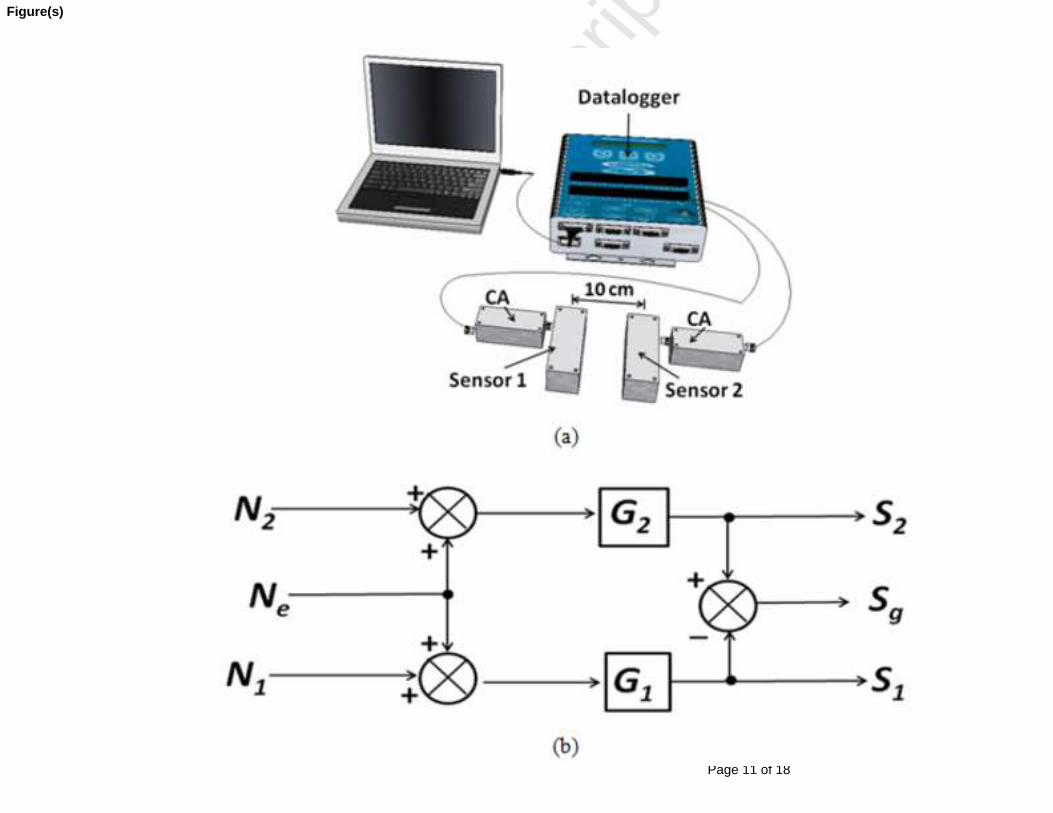
Figure 1. Schematic diagram of the Metglas/PZT ME laminate sensor. Figure 2(a) illustrates the configuration of sensors and signal collection electronics used in our experimentation. Two packaged ME laminate composite sensors and corresponding charge amplifier (CA) circuits were assembled into battery operated sensor detection units which were separated by a baseline of 10 cm. ME laminates were placed parallel to each other and aligned with the geomagnetic field. The charge amplifiers were designed with a transfer function of 1 V/pC and with a frequency bandwidth of 0.6 Hz to 10 Hz [15]. The output signals from the CAs were recorded using a CR5000 Datalogger (Campbell Scientific, Inc.) with a 100 Hz sample rate, a full-scale of 1 V and a dynamic range of 60 dB. Signal processing was carried out using MATLAB scripts. The noise tests were conducted in our lab (at about 10pm) which can be considered as a high magnetic and vibratory disturbance environment.

(a)

Page 3 of 18

Accep

ted

Man

uscr

ipt

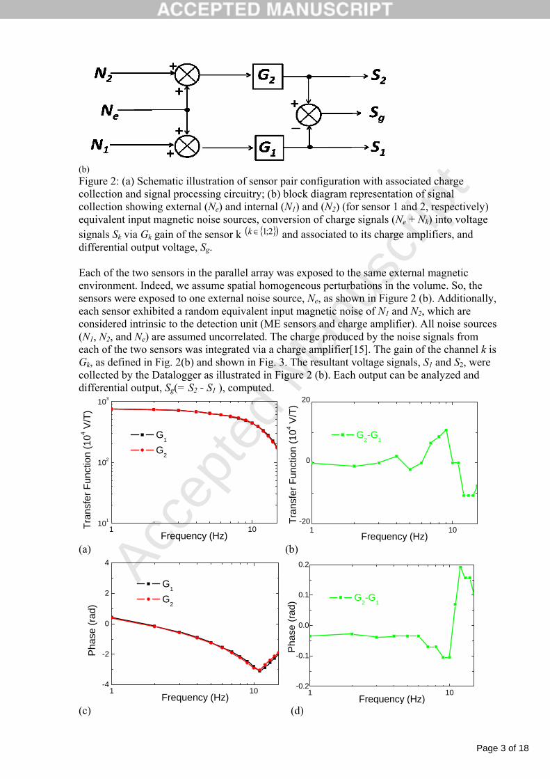
(b) Figure 2: (a) Schematic illustration of sensor pair configuration with associated charge collection and signal processing circuitry; (b) block diagram representation of signal collection showing external (Ne) and internal (N1) and (N2) (for sensor 1 and 2, respectively) equivalent input magnetic noise sources, conversion of charge signals (Ne + Nk) into voltage signals Sk via Gk gain of the sensor k { }( )2;1∈k and associated to its charge amplifiers, and differential output voltage, Sg. Each of the two sensors in the parallel array was exposed to the same external magnetic environment. Indeed, we assume spatial homogeneous perturbations in the volume. So, the sensors were exposed to one external noise source, Ne, as shown in Figure 2 (b). Additionally, each sensor exhibited a random equivalent input magnetic noise of N1 and N2, which are considered intrinsic to the detection unit (ME sensors and charge amplifier). All noise sources (N1, N2, and Ne) are assumed uncorrelated. The charge produced by the noise signals from each of the two sensors was integrated via a charge amplifier[15]. The gain of the channel k is Gk, as defined in Fig. 2(b) and shown in Fig. 3. The resultant voltage signals, S1 and S2, were collected by the Datalogger as illustrated in Figure 2 (b). Each output can be analyzed and differential output, Sg(= S2 - S1 ), computed.

1 10101

102

103

Tran

sfer

Fun

ctio

n (1

04 V/T

)

Frequency (Hz)

G1

G2

1 10

-20

0

20

Tran

sfer

Fun

ctio

n (1

04 V/T

)

Frequency (Hz)

G2-G1

(a) (b)

1 10-4

-2

0

2

4

Pha

se (r

ad)

Frequency (Hz)

G1

G2

1 10

-0.2

-0.1

0.0

0.1

0.2

Pha

se (r

ad)

Frequency (Hz)

G2-G1

(c) (d)

Page 4 of 18

Accep

ted

Man

uscr

ipt

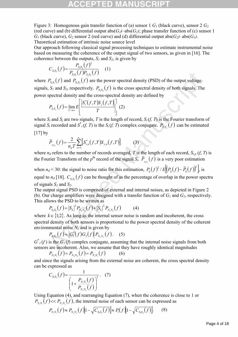
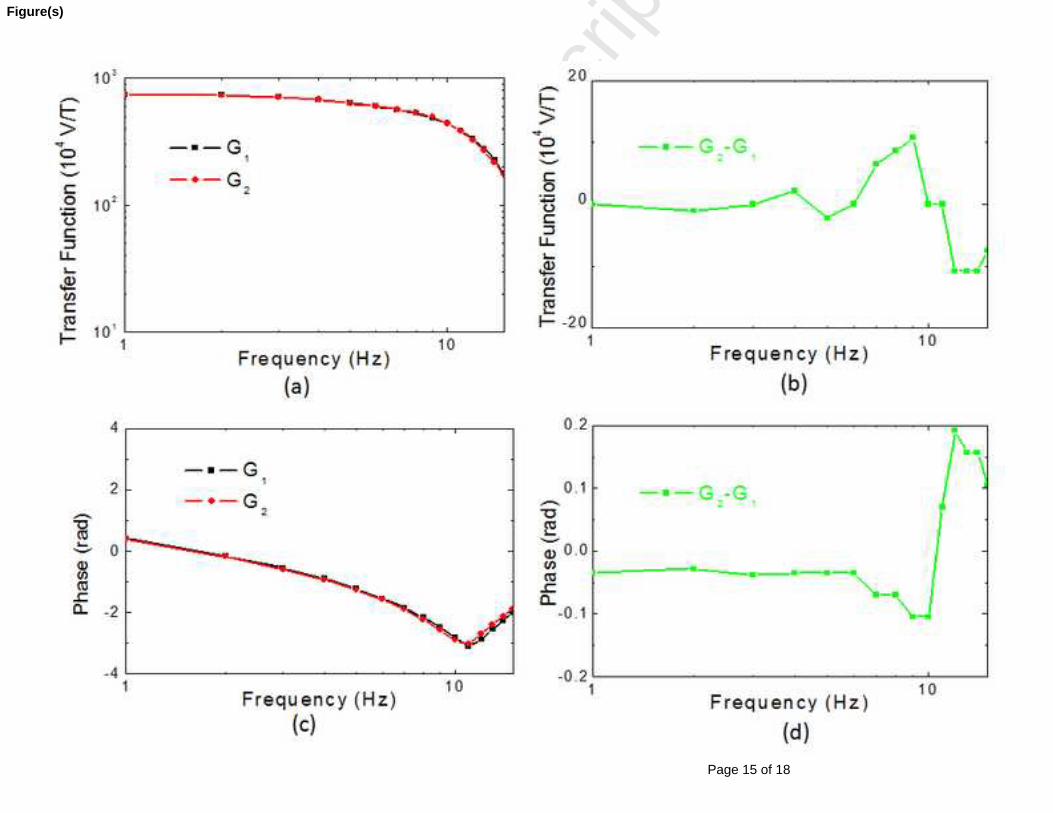
Figure 3: Homogenous gain transfer function of (a) sensor 1 G1 (black curve), sensor 2 G2 (red curve) and (b) differential output abs(G2)–abs(G1); phase transfer function of (c) sensor 1 G1 (black curve), G2 sensor 2 (red curve) and (d) differential output abs(G2)–abs(G1). Theoretical estimation of intrinsic noise source level Our approach following classical signal processing techniques to estimate instrumental noise based on measuring the coherence of the output signal of two sensors, as given in [16]. The coherence between the outputs, S1 and S2, is given by

( ) ( )( ) ( )fPfP

fPfC

SSSS

SSSS

2211

21

21

2

= (1)

where ( )fP SS 11 and ( )fP SS 22

are the power spectral density (PSD) of the output voltage signals, S1 and S2, respectively. ( )fP SS 21

is the cross spectral density of both signals. The power spectral density and the cross-spectral density are defined by

( )( ) ( )

⎥⎥⎦

⎤

⎢⎢⎣

⎡=

∞→ T

TfSTfSEfP ji

TSS ji

,,lim

*

(2)

where Si and Sj are two signals, T is the length of record, Si (f, T) is the Fourier transform of signal Si recorded and S*

i (f, T) is the Si (f, T) complex conjugate. ( )fPji SS can be estimated

[17] by

( ) ( ) ( )[ ]∑=

=d

jSiS

n

nnjni

d

TfSTfSTn

fP1

,*, ,,2~ (3)

where nd refers to the number of records averaged, T is the length of each record, Si,p (f, T) is the Fourier Transform of the pth record of the signal Si. ( )fP

jSiS

~ is a very poor estimation

when nd < 30: the signal to noise ratio for this estimation, ( ) ( ) ( )( )[ ]22 ~/ fPfPEfP ijijij − , is equal to nd [18]. ( )fC SS 21

can be thought of as the percentage of overlap in the power spectra of signals S1 and S2. The output signal PSD is comprised of external and internal noises, as depicted in Figure 2 (b). Our charge amplifiers were designed with a transfer function of G1 and G2, respectively. This allows the PSD to be written as ( ) ( ) ( )fPSfPSfP

eekkkk NNkNNkSS22 += (4)

where { }2;1∈k . As long as the internal sensor noise is random and incoherent, the cross spectral density of both sensors is proportional to the power spectral density of the coherent environmental noise Ne and is given by ( ) ( ) ( ) ( )fPfGfGfP

ee NNSS 2*121

= . (5) G*

1 (f ) is the G1 (f) complex conjugate, assuming that the internal noise signals from both sensors are incoherent. Also, we assume that they have roughly identical magnitudes ( ) ( ) ( )fPfPfP

ii NNNNNN ==2211

(6) and since the signals arising from the external noise are coherent, the cross spectral density can be expressed as

( )( )( )

2

1

121

⎟⎟⎠

⎞⎜⎜⎝

⎛+

=

fPfP

fC

ee

ii

NN

NN

SS . (7)

Using Equation (4), and rearranging Equation (7), when the coherence is close to 1 or ( ) ( )fPfP

eeii NNNN << , the internal noise of each sensor can be expressed as

( ) ( ) ( )[ ] ( ) ( )[ ]fCfPfCfPfP SSSSNNNN eeii 212111 1 −≈−≈ . (8)

Page 5 of 18

Accep

ted

Man

uscr

ipt

The gains of each channel are closed ( ) ( )( )fGfG 21 ≈ . Thus, the output noise in the differential configuration can be evaluated by

( ) ( ) ( ) ( ) ( )( ) ( )

⎟⎟

⎠

⎞

⎜⎜

⎝

⎛ −+= fP

fGfGfGfPfGfP

eeiigg NNNNSS

2

1

1221 2 . (9)

This noise level is clearly limited by the intrinsic differentiator noise, ( )fPii NN2 , and by

( ) ( )( ) ( )fPfG

fGfGee NN

2

1

12 − value given by the discrepancy between the two sensors (cf. Fig. 3).

In order to evaluate this last term, the ratio T12(f )=G2(f )/G1(f ) between S2(f ) and S1(f ) can be used

( ) ( )( ) ( ) ( ) ( )( )( )fTfTfTfG

fGfG1212

212

2

1

12 argcos21 −+=− . (10)

Then, for close sensors ( ε+= 112T with 1<<ε and ( ) 1arg 12 <<=θT ) and spatial homogeneous external noise sources, the rejection of coherent noise sources can be evaluated by

( ) ( )( )

222

1

12 θε +≈−fG

fGfG . (11)

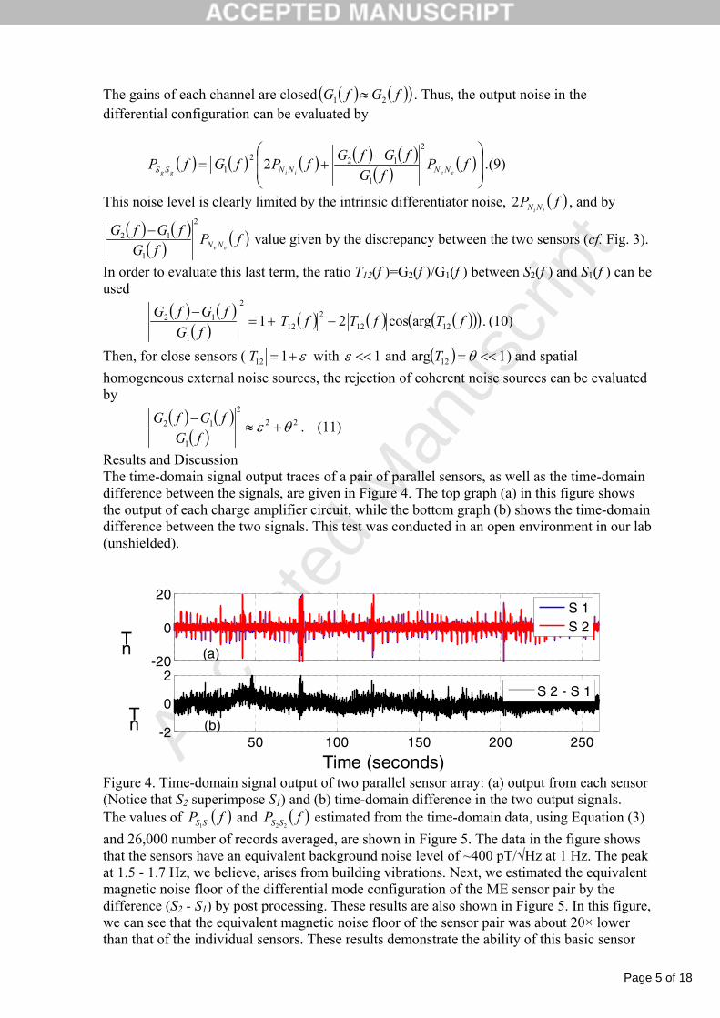
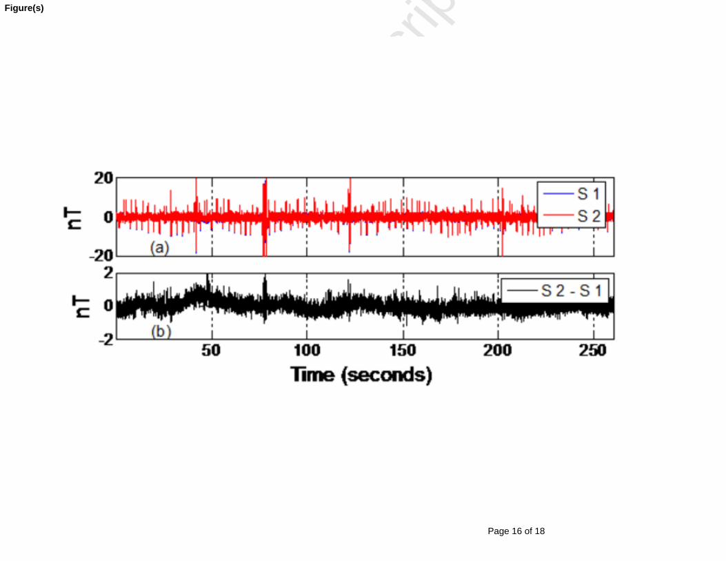
Results and Discussion The time-domain signal output traces of a pair of parallel sensors, as well as the time-domain difference between the signals, are given in Figure 4. The top graph (a) in this figure shows the output of each charge amplifier circuit, while the bottom graph (b) shows the time-domain difference between the two signals. This test was conducted in an open environment in our lab (unshielded).

-20

0

20

nT

S 1S 2

50 100 150 200 250-2

0

2

Time (seconds)

nT

S 2 - S 1

(b)

(a)

Figure 4. Time-domain signal output of two parallel sensor array: (a) output from each sensor (Notice that S2 superimpose S1) and (b) time-domain difference in the two output signals. The values of ( )fP SS 11

and ( )fP SS 22 estimated from the time-domain data, using Equation (3)

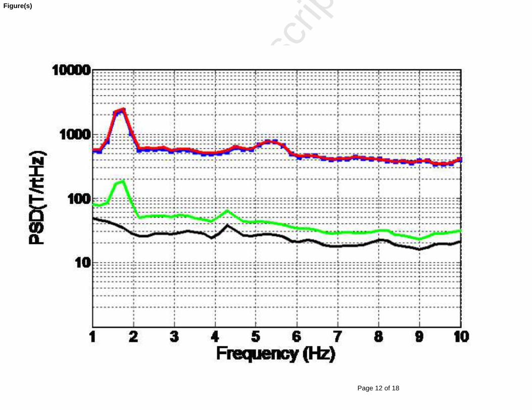
and 26,000 number of records averaged, are shown in Figure 5. The data in the figure shows that the sensors have an equivalent background noise level of ~400 pT/√Hz at 1 Hz. The peak at 1.5 - 1.7 Hz, we believe, arises from building vibrations. Next, we estimated the equivalent magnetic noise floor of the differential mode configuration of the ME sensor pair by the difference (S2 - S1) by post processing. These results are also shown in Figure 5. In this figure, we can see that the equivalent magnetic noise floor of the sensor pair was about 20× lower than that of the individual sensors. These results demonstrate the ability of this basic sensor

Page 6 of 18

Accep

ted

Man

uscr

ipt

differentiator to reject environmental noise, as a common mode. This infers a strong coherence between the output noise of S1 and S2.

1 2 3 4 5 6 7 8 9 10

10

100

1000

10000

Frequency (Hz)

PSD(T/rtHz)

Figure 5. Power spectral density curves of S1 (blue dotted curve), S2 (red curve) and the signal (S2 - S1) (green curve) after post processing. The estimated intrinsic sensor noise (N1 or N2) is the black curves. The upper plot (a) in Figure 6 shows the coherence ( )fC SS 21

between sensors 1 and 2. Because of ( ) 1

21≈fC SS , the ratio between S2 and S1 helps to evaluate the ratio

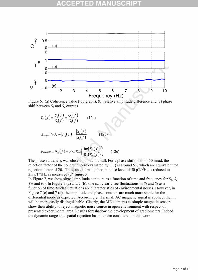
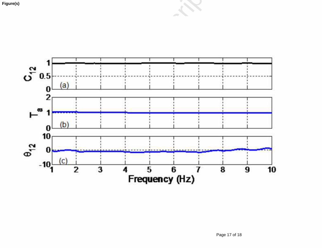
T12(f ) = G2(f )/G1(f ) as given in (12a). The magnitude of this ratio ( )fT12 gives information about the relative amplitudes of the output signals, while the phase of the transfer function θ12 provides information about the time lag between the two output signals. The middle plot (b) in Figure 6 originates from the smoothing transfer function amplitude ( )fT12 . As can been seen in this Figure 6, the amplitude remained at a near constant level of T12 = 1, which means that S1 and S2 have nearly identical absolute values. The phase angle θ12(f ) is shown in Figure 6 (c).

Page 7 of 18

Accep

ted

Man

uscr

ipt

0

0.5

1

C12

0

1

2

Ta

1 2 3 4 5 6 7 8 9 10-10

0

10

Frequency (Hz)

θ12

(a)

(b)

(c)

Figure 6. (a) Coherence value (top graph), (b) relative amplitude difference and (c) phase shift between S1 and S2 outputs.

( ) ( )( )

( )( )fG

fGfSfSfT

1

2

1

212 == (12a)

( ) ( )( )fS

fSfTAmplitude

1

212 =≡ (12b)

( ) ( )( )( )( )⎟

⎟⎠

⎞⎜⎜⎝

⎛=≡

fTfT

ArcTanfPhase12

1212 Re

Imθ (12c)

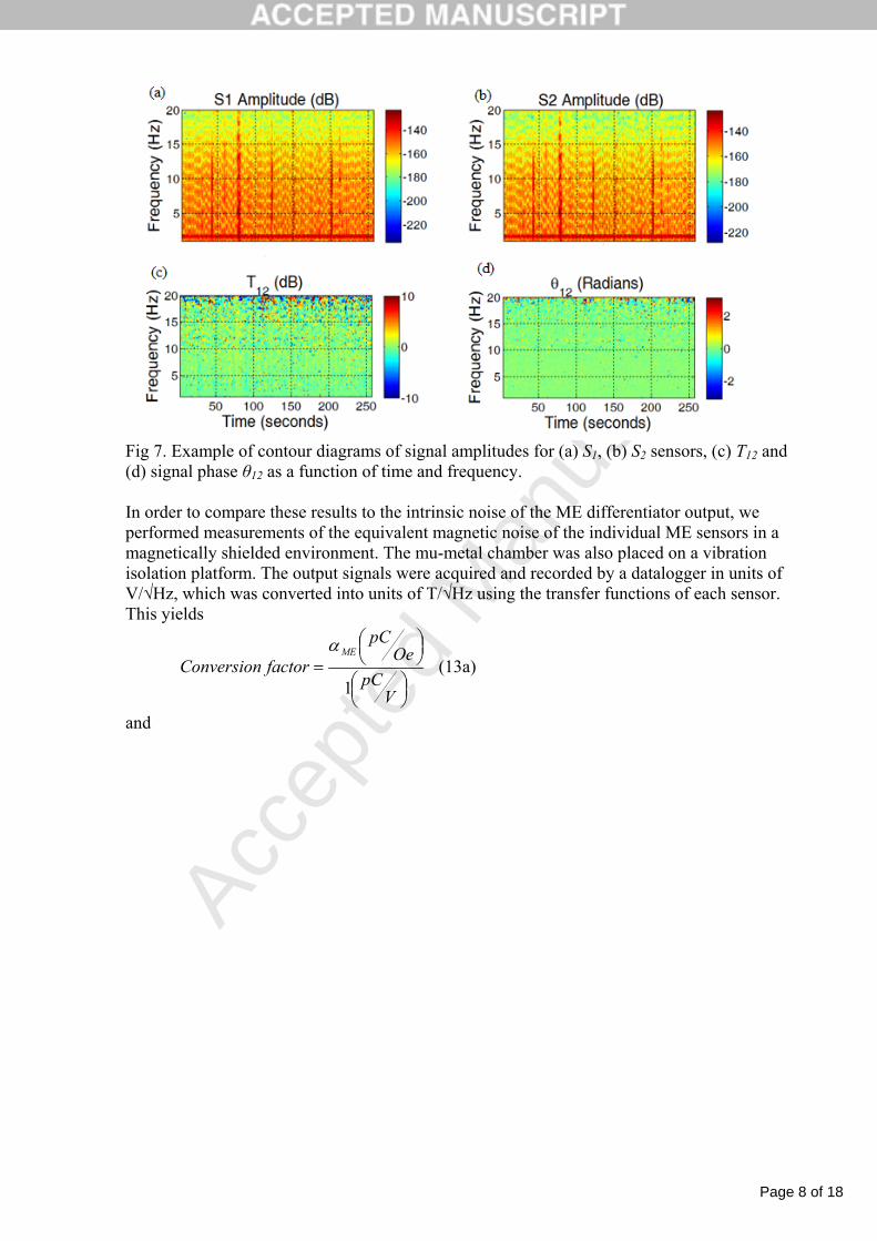
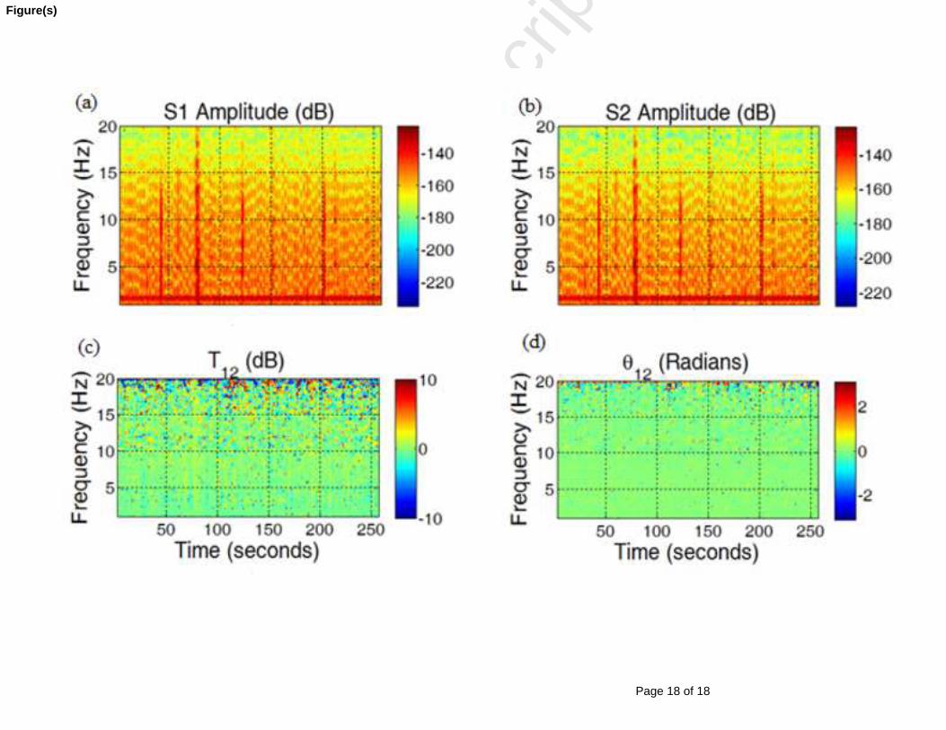
The phase value, θ12, was close to 0, but not null. For a phase shift of 3° or 50 mrad, the rejection factor of the coherent noise evaluated by (11) is around 5%,which are equivalent toa rejection factor of 20. Thus, an external coherent noise level of 50 pT/√Hz is reduced to 2.5 pT/√Hz as measured (cf. figure 5). In Figure 7, we show signal amplitude contours as a function of time and frequency for S1, S2, T12 and θ12. In Figure 7 (a) and 7 (b), one can clearly see fluctuations in S1 and S2 as a function of time. Such fluctuations are characteristics of environmental noises. However, in Figure 7 (c) and 7 (d), the amplitude and phase contours are much more stable for the differential mode as expected. Accordingly, if a small AC magnetic signal is applied, then it will be more easily distinguishable. Clearly, the ME elements as simple magnetic sensors show their ability to reject magnetic noise source in open environment with respect of presented experimental area. Results foreshadow the development of gradiometers. Indeed, the dynamic range and spatial rejection has not been considered in this work.

Page 8 of 18

Accep

ted

Man

uscr

ipt

Fig 7. Example of contour diagrams of signal amplitudes for (a) S1, (b) S2 sensors, (c) T12 and (d) signal phase θ12 as a function of time and frequency. In order to compare these results to the intrinsic noise of the ME differentiator output, we performed measurements of the equivalent magnetic noise of the individual ME sensors in a magnetically shielded environment. The mu-metal chamber was also placed on a vibration isolation platform. The output signals were acquired and recorded by a datalogger in units of V/√Hz, which was converted into units of T/√Hz using the transfer functions of each sensor. This yields

⎟⎠⎞⎜

⎝⎛

⎟⎠⎞⎜

⎝⎛

=

VpC

OepC

factorConversionME

1

α (13a)

and

Page 9 of 18

Accep

ted

Man

uscr

ipt

410−×⎟⎠⎞

⎜⎝⎛

=⎟⎠⎞

⎜⎝⎛

factorConversionHz

VfloorNoise

HzTfloorNoise . (13b)

1 2 3 4 5 6 7 8 9 10

10

100

1000

Frequency (Hz)

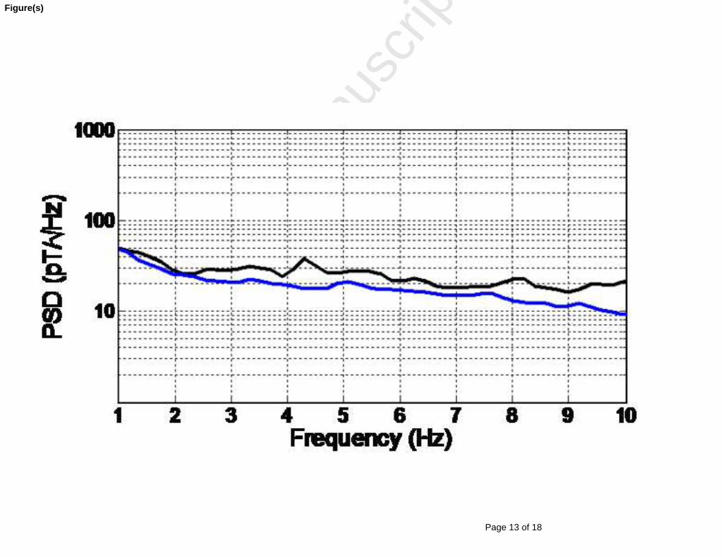
PSD (pT/√Hz)

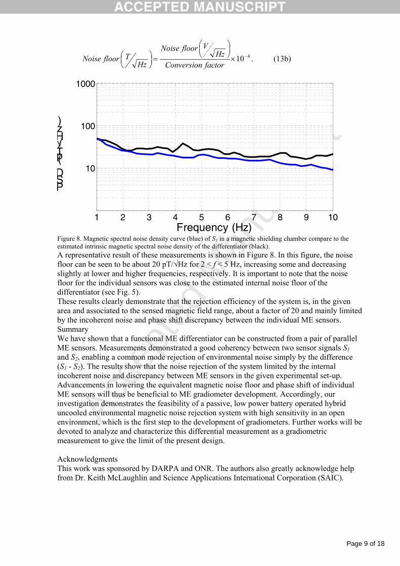
Figure 8. Magnetic spectral noise density curve (blue) of S1 in a magnetic shielding chamber compare to the estimated intrinsic magnetic spectral noise density of the differentiator (black). A representative result of these measurements is shown in Figure 8. In this figure, the noise floor can be seen to be about 20 pT/√Hz for 2 < f < 5 Hz, increasing some and decreasing slightly at lower and higher frequencies, respectively. It is important to note that the noise floor for the individual sensors was close to the estimated internal noise floor of the differentiator (see Fig. 5). These results clearly demonstrate that the rejection efficiency of the system is, in the given area and associated to the sensed magnetic field range, about a factor of 20 and mainly limited by the incoherent noise and phase shift discrepancy between the individual ME sensors. Summary We have shown that a functional ME differentiator can be constructed from a pair of parallel ME sensors. Measurements demonstrated a good coherency between two sensor signals S1 and S2, enabling a common mode rejection of environmental noise simply by the difference (S1 - S2). The results show that the noise rejection of the system limited by the internal incoherent noise and discrepancy between ME sensors in the given experimental set-up. Advancements in lowering the equivalent magnetic noise floor and phase shift of individual ME sensors will thus be beneficial to ME gradiometer development. Accordingly, our investigation demonstrates the feasibility of a passive, low power battery operated hybrid uncooled environmental magnetic noise rejection system with high sensitivity in an open environment, which is the first step to the development of gradiometers. Further works will be devoted to analyze and characterize this differential measurement as a gradiometric measurement to give the limit of the present design. Acknowledgments This work was sponsored by DARPA and ONR. The authors also greatly acknowledge help from Dr. Keith McLaughlin and Science Applications International Corporation (SAIC).

Page 10 of 18

Accep

ted

Man

uscr

ipt

Reference [1] R. Wiegert and J. Oeschger, "Portable magnetic gradiometer for real-time localization and classification of unexploded ordnance," IEEE , Oceans, 2006. [2] S. Kumar, et al., "Real-Time Tracking Magnetic Gradiometer for Underwater Mine Detection," IEEE , Oceans, 2004. [3] S. Kumar, et al., "Real-time tracking magnetic gradiometer for underwater mine detection," in OCEANS '04. MTTS/IEEE TECHNO-OCEAN '04, 2004, pp. 874-878 Vol.2. [4] J. Vrba, SQUID Sensors: Fundamentals, Fabrication and Applications. Dordrecht, Netherland: Kluwer Academic, 1996. [5] D. I. Gordon, "Recent Advances in Fluxgate Magnetometer," IEEE Transactions on Magnetics, vol. 8, 1972. [6] J. E. Lenz, "A review of magnetic sensors," Proceedings of the IEEE, vol. 78, pp. 973-989, 1990. [7] J. Zhai, "Geomagnetic sensor based on giant magnetoelectric effect," Applied Physics Letters, vol. 91, 2007. [8] S. X. Dong, et al., "Enhanced magnetoelectric effects in laminate composites of Terfenol-D/Pb(Zr,Ti)O-3 under resonant drive," Applied Physics Letters, vol. 83, pp. 4812-4814, Dec 2003. [9] S. Dong, et al., "Longitudinal and Transverse Magnetoelectric Voltage Coefficients of Magnetostrictive/ -Piezoelectric Laminate Composite: Theory," IEEE Trans. Ultrason. Ferroelectr. Freq. Control, vol. 50, p. 1253, 2003. [10] S. Dong, et al., "Push-pull mode magnetostrictive/piezoelectric laminate composite with an enhanced magnetoelectric voltage coefficient," Applied Physics Letters, vol. 87, p. 062502, 2005. [11] Z. Xing, et al., "Noise and scale effects on the signal-to-noise ratio in magnetoelectric laminate sensor/detection units," Applied Physics Letters, vol. 91, p. 182902, 2007. [12] J. Das, et al., "Enhancement in the field sensitivity of magnetoelectric laminate heterostructures," Applied Physics Letters, vol. 95, p. 092501, 2009. [13] B. Ullrich, et al., "Geophysical Prospection in the Southern Harz Mountains, Germany: Settlement History and Landscape Archaeology Along the Interface of the Latène and Przeworsk Cultures," Archaeological Prospection, vol. 18, pp. 95-104, 2011. [14] J. McGuirk, et al., "Sensitive absolute-gravity gradiometry using atom interferometry," Physical Review A, vol. 65, 2002. [15] Z. P. Xing, et al., "Modeling and detection of quasi-static nanotesla magnetic field variations using magnetoelectric laminate sensors," Measurement Science and Technology, vol. 19, p. 015206, 2008. [16] J. Bendat and A. Piersol, Random Data: Analysis and Measurement Procedures, 4th ed.: WILEY, 2010. [17] L. K. J. V. J. Briaire, "Uncertainty in Gaussian noise generalized for cross-correlation spectra," J. Appl. Phys, vol. 84, pp. 4370 - 4374, 1998. [18] P. Welch, "The Use of Fast Fourier Transform for the Estimation of Power Spectra: A Method of Time Averaging over Short Modified Periodograms," IEEE Trans. Audio and Electroacoustics, vol. 15, pp. 70-73, 1967.

Page 11 of 18

Accep

ted

Man

uscr

ipt

Figure(s)

Page 12 of 18

Accep

ted

Man

uscr

ipt

Figure(s)

Page 13 of 18

Accep

ted

Man

uscr

ipt

Figure(s)

Page 14 of 18

Accep

ted

Man

uscr

ipt

Figure(s)

Page 15 of 18

Accep

ted

Man

uscr

ipt

Figure(s)

Page 16 of 18

Accep

ted

Man

uscr

ipt

Figure(s)

Page 17 of 18

Accep

ted

Man

uscr

ipt

Figure(s)

Page 18 of 18

Accep

ted

Man

uscr

ipt

Figure(s)