Analysis of the Long-Term Pavement Performance Data for the … · 2013-03-13 · Analysis of the Long-Term Pavement Performance Data for the Idaho GPS and SPS Sections FINAL REPORT

Analysis of the Long-Term Pavement Performance Data for the Idaho GPS and SPS Sections

FINAL REPORT

NIATT Project No. KLK 481

ITD Project No. SPR-0003(014) RP 160

Prepared for

Idaho Transportation Department Mr. Michael Santi, PE

Assistant Material Engineer

Prepared by

Fouad Bayomy Professor of Civil Engineering and Principal Investigator

Hassan Salem

Graduate Research Assistant and

Lacy Vosti Undergraduate Research Assistant

National Institute for Advanced Transportation Technology Center for Transportation Infrastructure, CTI

University of Idaho

December 2006 (Revised June 2007)

i

ABSTRACT

This project addresses the analysis of the Long-Term Pavement Performance (LTPP) data for

the LTPP sites in Idaho. The goal was to determine the performance trends for the pavement

in Idaho as found in the LTPP experiments. The research also investigate into the use of the

data to develop (as much possible) models that enable the prediction of the seasonal variation

effects on the pavement materials (soils and asphalt mixes). In addition, the project looks into

the applicability of the LTPP data in Idaho for the use and implementation of the new

Mechanistic-Empirical Pavement design Guide (MEPDG).

Idaho participates in the LTPP program with 13 sites of general pavement studies

(GPS) that include GPS-1, 3, 5 and 6A experiments. There is only specific pavement studies

(SPS) experiment in Idaho (SPS-3). Idaho participates in the SPS-3 with 12 sections. All data

from all the sites were obtained and accumulated on a mini database. Analysis of the Idaho

data was supplemented with data from few LTPP sites located in adjacent states with similar

environments.

Analysis of the performance data including roughness and rutting revealed that

Continuous concrete pavements performed best, followed by jointed concrete pavements.

The asphalt pavements on granular bases and existing asphalt overlays on asphalt pavements

showed mediocre performances. That was largely due to the big gap in data at these sites.

For SPS sites regarding cracking and rutting, the various types of surface treatments tested at

the SPS 3 experiment were not effective at improving pavement conditions. Results showed

that to improve pavement roughness, a thin overlay is the best treatment option, followed by

the placement of a slurry seal coat. Placing chip and crack seal treatments did not show

significant impact on pavement roughness.

As part of the outcomes of this project, a mini-LTPP database for the LTPP sections

in Idaho was developed in MDB file format and series of Excel files that include all Idaho

data. In addition, models were developed based on analysis of national data for the subgrade

and asphalt concrete moduli. An investigation into the implementation of the MEPDG in

Idaho indicated that the current performance data in the Idaho sites are not sufficient for any

meaningful calibration of the performance models in the new design guide.

ii

ACKNOWLEDGEMENTS

This project was funded by the Idaho Transportation Department (ITD) under a contract with

the National Institute for Advanced Transportation Technology (NIATT), project number

KLK481. The ITD and FHWA supports are greatly appreciated.

Many Individuals have contributed to the progress of this project. From ITD, thanks are due

to Mr. Mike Santi, PE, Assistant Materials Engineer and Mr. Bob Smith, PE who oversaw

the project in its initial stages. Thanks are also due to Mr. Jeff Miles for his continued

support of our research program and his insight into the practicality of the research outcomes.

Many undergraduate students at the University of Idaho contributed at various stages to the

analysis of data in this report. In addition to the co-author of this report (Ms. Lacy Vosti),

Mr. Frank Eckwright has contributed a great deal of effort into the computer runs of the

Mechanistic-Empirical Design Guide software, and developed a worksheet to facilitate data

input. He contributed greatly to the writing of Chapter 7 of this report. In addition, Mr.

Ahmad Abu Abdo, a graduate student at UI, helped a lot in training the undergraduate

students. Thanks to all these individuals and their efforts are greatly appreciated.

The support of the NIATT administrative staff is also acknowledged. Ms. Judy LaLonde and

Debbie Foster have provided close monitoring for the project progress reports and budget.

Mr. Roger Saunders reviewed and edited the initial draft of the manuscript of the final report.

Authors are very thankful to all their efforts and support.

iii

TABLE OF CONTENTS 1. INTRODUCTION.................................................................................. 1

1.1 Background............................................................................................................... 1 1.2 Objectives ................................................................................................................. 2 1.3 Scope......................................................................................................................... 3 1.4 Methodology............................................................................................................. 4

2. IDAHO MINI LTPP DATABASE ....................................................... 5 2.1 LTPP dataBase.......................................................................................................... 5 2.2 LTPP sites in Idaho................................................................................................... 5 2.3 Mini Database ........................................................................................................... 6

3. REVIEW OF CURRENT DATA ANALYSIS REPORTS.............. 10 3.1 introduction............................................................................................................. 10 3.2 LTPP Smoothness And Distress Studies: A Review .............................................. 10 3.3 ROUGHNESS STUDIES ....................................................................................... 11

3.3.1 Factors Affecting Pavement Smoothness ....................................................... 11 3.3.2 Roughness Development of AC Pavements ................................................... 12 3.3.3 Roughness Development of PCC Pavements ................................................. 13 3.3.4 Roughness Characteristics of Overlaid Pavements......................................... 16 3.3.5 Models to Predict Roughness Development ................................................... 16 3.3.6 Transverse, Seasonal and Daily Variations of IRI.......................................... 17 3.3.7 Relationships Between IRI and Profile Index (PI) ......................................... 17

3.4 FLEXIBLE PAVEMENT MAINTENANCE EFFECTIVENESS......................... 26 3.4.1 Distress Variability ......................................................................................... 26 3.4.2 Description of LTPP Experiment SPS-3......................................................... 27 3.4.3 SPS-3 Performance Findings from Previous Studies...................................... 28 3.4.4 Effects of Flexible Pavement Maintenance Treatment on Roughness ........... 33 3.4.5 Effects of Flexible Pavement Maintenance Treatment on Rutting................. 35 3.4.6 Effects of Flexible Pavement Maintenance Treatment on Fatigue Cracking . 35

4. DATA MINING AND ANALYSIS – IDAHO DATA ...................... 37 4.1 INTRODUCTION .................................................................................................. 37 4.2 Selected SITES ....................................................................................................... 37 4.3 Methodology........................................................................................................... 39 4.4 Analysis................................................................................................................... 40

4.4.1 GPS-1: Asphalt Pavements On Granular Bases.............................................. 41 4.4.2 GPS-3: Jointed Concrete Pavements .............................................................. 45 4.4.3 GPS-5: Continuous Concrete Pavements........................................................ 47 4.4.4 GPS-6A: Existing Asphalt Overlays on Asphalt Pavements.......................... 50 4.4.5 SPS-3: Pavement Treatment Performance...................................................... 54

4.5 Conclusions form Idaho Sites ................................................................................. 58 4.5.1 GPS Sites ........................................................................................................ 58 4.5.2 SPS Sites ......................................................................................................... 58

iv

5. SEASONAL VARIATION OF SUBGRADE RESILIENT MODULUS – NATIONAL LTPP DATA ...................................................................... 59

5.1 INTRODUCTION .................................................................................................. 59 5.2 Backgorund on the LTPP SMP Study .................................................................... 59 5.3 modulus-moisture relationship for subgrade soils .................................................. 61

5.3.1 Moisture Effects on Soil Resilient Modulus................................................... 61 5.3.2 Temperature Effects on Subgrade Soil Resilient Modulus............................. 63 5.3.3 Subgrade Moisture Prediction Using the Integrated Climatic Model (ICM) . 64 5.3.4 Seasonal Variation and Seasonal Adjustment Factors.................................... 65

5.4 LTPP-SMP DATA requisition and preparation...................................................... 66 5.5 DATA ANALYSIS................................................................................................. 67

5.5.1 Moisture and Modulus Variation with Time .................................................. 68 5.5.2 Model Development for Plastic Soils ............................................................. 68 5.5.3 Estimating Seasonal Adjustment Factors........................................................ 73

5.6 Conclusions of SMP Data Analysis for Subgrade Soils ......................................... 78 6. SEASONAL VARIATION OF THE ASPHALT CONCRETE MODULUS – NATIONAL LTPP DATA................................................. 79

6.1 INTRODUCTION .................................................................................................. 79 6.2 modulus-Temperature relationship for AC layer.................................................... 79

6.2.1 Seasonal Variations in the AC Layer Elastic Modulus................................... 79 6.2.2 Relating Temperature Variation to AC Modulus............................................ 80 6.2.3 Pavement Temperature Prediction Models..................................................... 81

6.3 LTPP DATA ACQUISITION and preparation ...................................................... 82 6.3.1 DATA ANALYSIS......................................................................................... 84 6.3.2 Temperature and Modulus Variation with Time ............................................ 84 6.3.3 AC Layer Temperature at Various Depths Versus Modulus .......................... 84 6.3.4 AC Modulus Versus Mid-Depth Temperature ............................................... 86 6.3.5 AC Layer Modulus Prediction Models ........................................................... 91 6.3.6 Estimating the Seasonal Adjustment Factor ................................................... 94

6.4 Conclusions of the SMP Data Analysis for Aspahlt Modulus................................ 96 7. APPLICABILITY OF THE IDAHO LTPP DATA FOR THE IMPLEMENTATION OF MEPDG.......................................................... 98

7.1 Introduction............................................................................................................. 98 7.2 Backgorund on the MEPDG ................................................................................... 98 7.3 MEPDG Inputs and Availability in the LTPP Database for Idaho......................... 99 7.4 Recommendation for Implementation at the State level....................................... 100

8. CONCLUSIONS ................................................................................ 106 9. REFERENCES................................................................................... 109 10. APPENDICES .................................................................................... 116

v

LIST OF FIGURES

Figure 2-1: LTPP Sites in Idaho ............................................................................................... 7 Figure 2-2 GPS and SPS Sites in Neighboring States that were Used in Analysis ................. 8 Figure 3-1: Relationship between the inertial profiler IRI and the PI5-mm (PI0.2-in) .......... 18 Figure 3-2: Relationships between the profilograph PI5-mm (PI0.2-in) and the IRI values.. 21 Figure 3-3: Relationships between the IRI and the simulated PI response............................. 22 Figure 3-4: Correlation analysis of the IRI and simulated PI5-mm (PI0.2-in) values produced by the lightweight profiler. ..................................................................................................... 24 Figure 4-1: GPS-1 Roughness Trends in Idaho ...................................................................... 42 Figure 4-2: GPS-1 Rutting Trends in Idaho............................................................................ 43 Figure 4-3: GPS-3 Roughness Trends in Idaho ...................................................................... 46 Figure 4-4: GPS-3 Rutting Trends in Idaho and Washington................................................. 47 Figure 4-5: GPS-5 Roughness Trends in Idaho ...................................................................... 48 Figure 4-6: GPS-5 Rutting Trends in Idaho and Oregon........................................................ 49 Figure 4-7: GPS-6A Roughness Trends in Idaho ................................................................... 51 Figure 4-8: GPS-6A Rutting Trends in Idaho, Washington and Wyoming............................ 52 Figure 5-1: Variation of Modulus and Moisture with Time for Various Soil Types at the Selected LTPP Sites................................................................................................................ 69 Figure 5-2: Model Development for Non-Plastic Soils .......................................................... 72 Figure 5-3: Modulus-Moisture Relationships for Non-Plastic Soils. ..................................... 75 Figure 5-4: Variation of the Seasonal Adjustment Factor with the Moisture Ratio for Different Soil Types................................................................................................................ 77 Figure 6-1: Variation of Modulus and Temperature with Time for Three Different LTPP Sites......................................................................................................................................... 85 Figure 6-2: Modulus Versus Pavement Temperature at Various Depths. .............................. 87 Figure 6-3: Modulus - Temperature Relationship for Five Sites from Nonfreezing Zones. .. 88 Figure 6-4: Modulus – Temperature Relationship for Six Sites from Freezing Zones .......... 90 Figure 6-5: Comparing The Models to Data from Different Zones........................................ 93 Figure 6-6: Estimated AC Layer Modulus Shift Factor for Both Nonfreezing and Freezing Zones....................................................................................................................................... 96

vi

LIST OF TABLES

Table 2-1: Available LTPP Sites in Idaho and Their Locations............................................... 9 Table 2-2: Selected sites in Neighboring States that were used in the Analysis ...................... 9 Table 3-1: The various regression equations found in the literature relating IRI from an inertial profiling system with PI statistics (PI5-mm, PI2.5-mm, and PI0.0) , Kelly et al. (2002)...................................................................................................................................... 25 Table 3-2: SPS-3 Core Experimental Sections. ...................................................................... 27 Table 4-1: Pavement Information for GPS-1 Sites ................................................................. 37 Table 4-2 Climatic Information for GPS and SPS Sites in Idaho........................................... 38 Table 4-3: Pavement Information for GPS-3, 5, 6A and SPS-3 Sites .................................... 38 Table 4-4: Specific Location and Climate Information for Non-Idaho Sites ......................... 39 Table 4-5: Pavement Information for Non-Idaho Sites .......................................................... 39 Table 5-1: Experimental Design and Data Elements for the LTPP Seasonal Monitoring Program (Rada et al, 1994) ..................................................................................................... 60 Table 5-2: Selected LTPP Sites and Subgrade Soil Characterizations ................................... 67 Table 5-3: SAS Output for Regression Analyses for Modulus-Moisture Relationship for Plastic Soils............................................................................................................................. 71 Table 5-4: SAS Output for Regression Analyses for Modulus-Moisture Relationship for Non-Plastic Soils............................................................................................................................. 74 Table 5-5: Parameters k1 and k2 for the SAF Model (Equation 7) ........................................ 76 Table 6-1: Selected LTPP Sites and Their AC Layer Properties............................................ 82 Table 6-2: Estimated Constants of The Exponential Function for The different Sites........... 89 Table 7-1 Example of Inputs for the MEPDG Using Data from Idaho Site 16-1001 .......... 101

1

1. INTRODUCTION

1.1 BACKGROUND

Pavement performance is a critical factor in the operation, planning, and engineering of

highway facilities. It affects the safety and comfort of the highway user. It is also an

economic factor in that engineers want to extend the pavement life to the most economical

extent possible. Understanding "why" some pavements perform better than others is key to

building and maintaining a cost-effective highway system. That's why in 1987, the Long-

Term Pavement Performance (LTPP) program - a comprehensive 20-year study of in-service

pavements - began a series of rigorous long-term field experiments monitoring more than

2,400 asphalt and Portland cement concrete pavement test sections across the U.S. and

Canada. LTPP was designed as a partnership with the States and Provinces. One of its goals

was to help the States and Provinces make decisions that will lead to better performing and

more cost-effective pavements.

The LTPP research program is an outgrowth of the Strategic Highway Research Program

(SHRP) which initiated the original LTPP program in 1987 to study the long-term

performance of the in-service pavements. At the completion of SHRP program, in 1992, the

Federal Highway Administration (FHWA) continued and expanded the LTPP program.

Under FHWA, a seasonal monitoring program (SMP) was initiated within the LTPP program

to focus on the effects of seasonal changes on pavement performance. Data collected from

the various studies in the LTPP program are accessible via the LTPP Datapave online web

site (http://www.ltpp-products.com/DataPave/index.asp), which allows access to almost all

data in the national LTPP database.

The Idaho Transportation Department (ITD) is sponsoring research into the pavement

performance specific to the state of Idaho. Such specific research is needed to understand the

seasonal changes on a number of pavement types in the state. This report is a compilation of

University of Idaho research into the data collected on pavements in Idaho, in particular, and

the uses of national pavement data for modeling pavement performance, in general.

2

Specifically, this research project focuses on the analysis of the data from LTPP sits in Idaho.

The Idaho sites include 13 general pavement studies (GPS) sites. The GPS experiments in

Idaho are GPS-1 (9 sites), GPS-3 (2 sites), GPS-5 (one site) and GPS-6A (one site). All these

experiments are studies of in-service asphalt concrete pavements. GPS-1 sites are asphalt

pavements built on granular bases, GPS-3 sites are for jointed concrete pavements, GPS- 5

site is for continuous concrete pavement, and the GPS-6A site is for existing asphalt overlay

over asphalt pavement.

Idaho also participates in the LTPP specific pavement studies (SPS) in the experiment of

preventive maintenance effectiveness for asphalt pavements designated as SPS-3. The SPS-3

experiment design matrix, in Idaho, includes 12 sections, which are located in three sites.

Each site is divided into four sections for different treatment methods (crack seal, chip seal,

slurry seal and thin overlay). Data have been collected by both the state and the FHWA-

LTPP program. However, very limited analysis has been done to address pavement

performance problems specific to the state conditions. The SPS-3 experiments are of great

importance since they address current maintenance techniques adopted by ITD. Analysis of

data available in the LTPP information management system (IMS) shall help the state

evaluates the effectiveness of these techniques in Idaho environment.

This project represents the only activity related to data analysis of the Idaho LTPP sections at

the state level. At the national level, there are few NCHRP projects that address LTPP data

analysis. However, the NCHRP projects are neither particular nor focused on the Idaho

sections, especially that there is no current NCHRP project for preventive maintenance.

Review of all previous data analysis reports developed by FHWA contractors or by NCHRP

contractors is presented later in this report.

1.2 OBJECTIVES

The overall objective of this project is to analyze the LTPP data related to the Idaho sections

for the following purposes:

3

• Develop a mini-database that includes Idaho LTPP data.

• Study the performance characteristics of pavements in Idaho in general and the

effectiveness of the preventive maintenance techniques used in the Idaho SPS-3 sites.

• Develop pavement performance models, as far as the data allows. These models

should incorporate the effect of pavement structure, material properties, and

environment and traffic loading conditions.

• Investigate how the Idaho LTPP data can support the implementation of the new

Mechanistic-Empirical Pavement Design Guide (MEPDG) that is expected to be

adopted by AASHTO in the near future.

1.3 SCOPE

The scope of this project is limited to procure all LTPP data for Idaho sections from the

national database via the DataPave software. Analyze the data to develop performance

trends, and investigate the applicability of previously developed models, or established trends

from the national studies, to the pavement sections in Idaho. As mentioned earlier, the

majority of GPS sections in Idaho are for the GPS-1 experiment. Thus, the focus is on the

performance characteristics of pavements built on granular bases, which is the main feature

of the pavements in GPS-1 experiment. For the Specific Pavement Studies (SPS) sections,

only sections for the SPS-3 (Preventative Maintenance Effectiveness) experiment are

available in Idaho. While all data will be analyzed, the focus is on developing performance

trends for:

• Smoothness or Roughness variability, • Distress development.

The variability of these performance indicators may be investigated in relation to:

• Structural support parameters (layer thicknesses and elastic moduli) • Site conditions, such as freeze or non-freeze, dry or wet.

For the SPS sections, the target is to identify how significant are the various maintenance

techniques adopted at these sections.

4

1.4 METHODOLOGY

The following tasks were undertaken to address the objectives and scope of the project:

Task 1: Develop Idaho Mini LTPP Database: All LTPP data related to Idaho sections

was procured from the national IMS. It was done by means of DataPave software. At early

stages of the project, DataPave version 3.0 was used, and when the FHWA moved to the

online version, data was acquired via the DataPave online. In addition, Microsoft Access

Database files were procured directly from LTPP headquarters. LTPP general data release

and management protocols were followed. The procured data was collected in one mini-

database (in series of Excel files) to facilitate analysis. The database also includes the MS-

Access files for future reference. In addition to the raw data files, analyzed data are also

included in the various database files. The files are provided in electronic format on a CD.

Task 2: Review Current Data Analysis Reports: Relevant reports published by

FHWA and NCHRP were reviewed to establish a methodology for the analysis.

Task 3: Data Mining and Analysis: The collected data was analyzed using basic

statistical tools. The data was analyzed to establish performance trends, and investigate the

level of its applicability to available performance models.

Task 4: Develop an Implementation Plan for new AASHTO 2002 Design Guide,

which is referred to later as the Mechanistic-Empirical Pavement Design Guide (MEPDG).

Depending upon the released information on the AASHTO 2002 design guide and as much

as the data available allowed, the analyzed data was used to determine its applicability for the

use in the MEPDG.

This report was prepared to address the results of these tasks, and document the conclusions

of the data analysis. The following chapters are organized to address the tasks listed above.

5

2. IDAHO MINI LTPP DATABASE

2.1 LTPP DATABASE

The LTPP program includes more than 2400 sites in North America. These sites include

about 800 GPS sites and about 1600 SPS sites. The national database of all these sites is

housed in a central database, referred to the Information Management system, IMS), which

that is accessible via the DataPave online software. The national database includes more than

500 in 22 modules with thousands of data fields. Additional data are stored offline, which

can be accessed via the LTPP headquarters. However, these additional data files are massive

and are not needed for many of the analysis purposes. For example, there is a separate central

traffic database that houses all the traffic data that states provide to the LTPP. Summary of

the traffic information is stored in the national main IMS. The database is updated annually

since the data collection process is a continuous process since the launch of the LTPP

program. For the majority fo data users, data can be obtained from the DataPave Online.

2.2 LTPP SITES IN IDAHO

The state of Idaho participates in the FHWA long-term pavement performance (LTPP)

program, with 13 general pavement studies (GPS) sites. The GPS experiments in Idaho are

GPS-1 (9 sites), GPS-3 (2 sites), GPS-5 (one site) and GPS-6A (one site). All these

experiments are studies of in-service asphalt concrete pavements. GPS-1 sites are asphalt

pavements built on granular bases, GPS-3 sites are for jointed concrete pavements, GPS-5

site is for continuous concrete pavement, and the GPS-6A site is for existing asphalt overlay

over asphalt pavement. Also, the state participates in the LTPP specific pavement studies

(SPS) in the experiment of preventive maintenance effectiveness for asphalt pavements

designated as SPS-3. The SPS-3 experiment design matrix, in Idaho, includes 12 sections,

which are located in three sites. Each site is divided into four sections for different treatment

methods (crack seal, chip seal, slurry seal and thin overlay). Figure 2-1 shows the different

site locations in Idaho.

6

The main sites specific information like; the site latitude, longitude, elevation, highway class,

route number, county located in, construction date, freezing index, average precipitation and

number of days above 32 C are all presented in Table 2-1.

Due to limited data for some experiments, two GPS-5 sites in Oregon and two GPS-6A sites

from both Washington and Wyoming were used in the data analysis of some criteria. The

location of these GPS and SPS sites can be seen in Figure 2-2 while specific site information

for non-Idaho sites are presented in Table 2-2

2.3 MINI DATABASE

For the purpose of this project, all data in the LTPP Database for all Idaho sites have been

obtained and updated. The versions of the data release that were used to retrieve LTPP data

for the analysis in this project included the DataPave 3 that was released in 2002, and

subsequent standard data release versions 17, 18, 19 and 20 for the years 2003, 2004, 2005,

and 2006.

All data retrieved from the LTPP Database were accumulated in one single MS-Access

database file, and stored in a folder named “ID_LTTP Mini Database” and is provided in

the project CD (attached to this report). The main database file (ID_LTPP Data.mdb)

includes all the raw data from LTTP tables. The tables in this file are structured in

accordance to the LTPP table structure system. To facilitate the identification of all tables

and codes, a (CODE.mdb) file is also included. The traffic data tables from the LTPP

database for all sections in Idaho are included in the file (ID_Traffic.mdb). The user will

need to use the MS-Access Database software to open these database files.

In addition, all files for the data analysis are presented in series of Excel sheets and charts.

They are grouped and stored in the same folder “ID_LTPP Mini Database”.

7

Figure 2-1: LTPP Sites in Idaho

9034

N GPS-1 (9 Sites)

GPS-3 (2 Sites)

GPS-5 (1 Site)

GPS-6A (1 Site)

SPS (3x3 = 9Sites)

Idaho Sites (5)

1001

9032

1005

1009

1020

1007 5025

3017

6027

1021

SPS_B SPS_C

1010 SPS_A

3023

8

Figure 2-2 GPS and SPS Sites in Neighboring States that were Used in Analysis

9

Table 2-1: Available LTPP Sites in Idaho and Their Locations

1001 8/1/1973 Kootenai 2 95 2150 47.77 116.79 217 692.9 16.081005 7/1/1975 10/1/1999 Adams 2 95 3232 44.63 116.44 399.1 627 44.861007 6/1/1972 8/1/1997 Twin Falls 2 30 3771 42.59 114.7 326 253.8 23.96

1009 10/1/1974 Cassia 1 84 3025 42.47 113.38 350.61 261.77 29.131010 10/1/1969 8/1/1997 Jefferson 1 15 4775 43.68 112.12 665.21 303.42 19.041020 9/1/1986 Jerome 2 93 4097 42.74 114.44 327.59 280.01 42.121021 10/1/1985 Jefferson 2 20 4849 43.65 111.93 622 341.55 17.249032 10/1/1987 Kootenai 2 95 2602 47.64 116.87 258.65 717.98 10.59

3017 9/1/1986 Power 1 86 4254 42.64 113.05 356.24 341.82 47.35

SPS3320: Slurry

330: Crack B Jefferson 2 20 4849 43.65 111.93 622 341.55 17.24

350: Chip C 8/1/1997 Jefferson 1 15 4775 43.68 112.12 665.21 303.42 19.04

327.59 280.01 42.12

De-Assign date

Route # Elev, (m)

Freez Index (C-Days)

5

A Jerome 2 93 4097 42.74 114.44

42.45 111.35 817.16 379.77Bear Lake 2 30 6056GPS6A 6027 9/1/1960 8/1/1997

112.21 538.28 399.28 21.92

47.59

GPS5 5025 9/1/1972 8/3/1995 Bannock 1 15 4979 42.38

43.84 116.76 278.29 295.29Payette 1 84 2503GPS3

3023 10/1/1983

116.5 315.53 806.69 9

Days above 32 C

GPS1

9034 10/1/1988 Bonner 2 95 2119 48.42

Class Lat, Deg Long, Deg

Precipit. (mm)

Experiment Site Const. Date

County

Table 2-2: Selected sites in Neighboring States that were used in the Analysis

Experiment State SiteRoute Number

Functional Class Elev. (ft) ecipitation (Freezing Index (C‐days)

Climatic Region

GPS‐1 WA 1002 12 Rural Arterial 1557 18.7 155.7 Dry FreezeGPS‐3 WA 3013 195 Rural Arterial 2356 17 292.1 Dry FreezeGPS‐5 OR 5008 84 Rural Interstate 2729 17.2 179.8 Dry Freeze

UT 7082 15 Rural Interstate 4527 16.7 411.45 Dry FreezeWA 6056 195 Rural Arterial 2545 19.9 175.3 Dry FreezeWA 7322 195 Rural Arterial 2545 21.1 224.5 Wet FreezeWY 6032 22 Rural Mjr. Collector 6156 17.5 894.3 Dry FreezeGPS‐6A

10

3. REVIEW OF CURRENT DATA ANALYSIS REPORTS

3.1 INTRODUCTION

This chapter discusses the previous research done related to the objectives of this project

through a comprehensive literature review of previous roughness and distress studies and the

effectiveness of the flexible pavement maintenance. Appendix A contains a bibliography of the

related FHWA and NCHRP Reports indicating which were reviewed for use.

3.2 LTPP SMOOTHNESS AND DISTRESS STUDIES: A REVIEW

The original Long-Term Pavement Performance (LTPP) program was established by the

Strategic Highway Research Program (SHRP) in 1987 to study the long-term performance of the

in-service pavements. The objective of the LTPP program and its state of progress since its

inception has been the subject of many publications. The original SHRP-LTPP program included

two main experiments, the General Pavement Studies (GPS) and the Specific Pavement Studies

(SPS). At the conclusion of the SHRP in 1992, the LTPP program continued under the

management of the Federal Highway Administration (FHWA). The FHWA-LTPP program team

recognized the need to study the environmental impacts on pavement performance.

Consequently, the FHWA-LTPP team launched the Seasonal Monitoring Program (SMP) as an

integral part of the LTPP program. The primary objective of the SMP was to study the impacts of

temporal variations in pavement response and materials properties due to the separate and

combined effects of temperature, moisture and frost/thaw variations. The GPS sections generally

represent pavements that incorporate materials and structural designs used in standard

engineering practice in the United States. The GPS test sections had been in service for some

time when they were accepted into the LTPP program. Roughness data collection at these test

sections has been performed at regular intervals after the test sections were accepted into the

LTPP program. However, the initial International Roughness Index (IRI) of these test sections

are not known. The SPS experiments were designed to study the effect of specific design features

on pavement performance. Each SPS experimental test site consists of multiple test sections,

each of which is 152 m in length.

11

3.3 ROUGHNESS STUDIES

Several research projects that used LTPP data to study roughness progression have been

performed during the past several years. Perera et al. (1998) had performed the first

comprehensive analysis of roughness progression at LTPP sections. He investigated the time-

sequence roughness data at GPS test sections to study trends in development of roughness, and

developed models to predict roughness. An evaluation of roughness data collected for the SPS-1,

-2, -5 and –6 experiments were also performed. Khazanovich et al. (1998) used LTPP data to

investigate common characteristics of good and poorly performing PCC pavements. They

grouped jointed plain concrete (JPC), jointed reinforced concrete (JRC) and continuously

reinforced concrete (CRC) pavements into three groups (poor, normal and good) based on time

vs IRI relationships, and examined factors contributing to differences in pavement performance.

Owusu-Antwi et al. (1998) and Titus-Glover et al. (1998,1999) used LTPP data to analyze the

performance of PCC pavements. They determined design features and construction practices that

enhance pavement performance, and developed models to predict roughness. Simpson et al.

(1994) performed a sensitivity analysis of IRI data at the GPS sections.

Profile data collected at GPS-3 and 4 sections were analyzed by Byrum (2000). This research

developed a curvature index to quantify slab shape from profile elevation data, and showed that

slab curvature was related to PCC pavement performance. An analysis of pavement performance

trends for test sections in SPS-5 and SPS-6 projects was also performed by Daleiden et al.

(1998). In this study, a comparison of performance trends of different test sections was made to

evaluate the effect of different rehabilitation treatments. The parameters studied were pavement

distress (e.g., fatigue cracking, longitudinal cracking, transverse cracking), roughness, rutting,

and deflection data. Von Qunitus et al. (2000) used LTPP data to study the relationship between

changes in pavement surfaces distress of flexible pavements to incremental changes in IRI.

3.3.1 Factors Affecting Pavement Smoothness

The data available in the LTPP Information Management System (IMS) was used by Perera and

Kohn (2001) to determine the effect of design and rehabilitation parameters, climatic conditions,

12

traffic levels, material properties, and extent and severity of distress that cause changes in

pavement smoothness. The IRI was used as the measure of pavement smoothness.

The pavement types in the GPS experiment that were studied in this research project were:

asphalt concrete (AC) on granular base, AC on stabilized base, jointed plain concrete, jointed

reinforced concrete, continuously reinforced concrete, AC overlays of AC pavements, and AC

overlays on concrete pavements. Roughness trends over time for each of these pavement types

were studied. Subgrade, climatic and pavement material properties that influence the roughness

progression on each of these pavement types were identified.

In their final report, Perera and Kohn (2001) concluded that the cause for the high rate of

increase of roughness that were observed on some of the sections prior to the end of their design

life can be attributed to several causes. If a pavement is subjected to its design traffic volume in a

time period that is less than its intended design life, the roughness of the section is expected to

increase rapidly. Also, if the pavement is not adequately designed based on the subgrade and

environmental conditions at the site, the roughness of the section can increase at a high rate. It

was noted that the pavements that are at higher levels of roughness generally were subjected to a

several factors that were identified to be causing high roughness levels. There were many

sections that were old, but have maintained their smoothness level over time. Many of these

sections appear to have carried low traffic volumes relative to the theoretical traffic volume that

can be carried by the pavement section. It was observed that pavements that were of similar age

show a parallel trend in roughness progression, indicating pavements that are built smoother

provide a smoother pavement over its design life.

3.3.2 Roughness Development of AC Pavements

Perera et al. (1998) found a strong relationship between pavement performance and

environmental factors. Each of their GPS sections had been profiled an average of four times.

When roughness progression for test sections in each GPS experiment was plotted for each of the

four environmental zones (i.e., wet-freeze, wet no-freeze, dry-freeze, and dry no-freeze), there

were distinct trends in roughness progression between the regions. The observed roughness

13

development trends in GPS-1 sections seem to indicate that pavement roughness remains

relatively constant over the initial life of the pavement and then after a certain point show a rapid

increase. The IRI plots show several sections that were over 15 years old, but had low IRI values.

An analysis of these sections indicated they have carried a relatively low cumulative traffic

volume when compared to the theoretical cumulative traffic volume the section was capable of

carrying. A preliminary analysis of the sections showing a high increase in roughness over the

monitored period indicated that these sections were close to or exceeded their design life based

on equivalent axle loads.

3.3.3 Roughness Development of PCC Pavements

A comprehensive analysis of IRI trends of GPS-3, GPS-4 and GPS-5 pavements was performed

by Perera et al. (1998). This analysis indicated distinct IRI trends for each of those experiments.

Perera et al. (1998) found that for JPC pavements (i.e., GPS-3) there were distinct differences in

IRI progression between doweled and non-doweled pavements. Generally, the non-doweled

pavements showed higher rates of increase in roughness when compared to doweled pavements.

For both doweled and non-dowelled pavements, higher IRI values were generally indicated for

pavements located in areas that received higher precipitation, had higher freezing indices, and

had a higher content of fines in the subgrade. In the non-freeze regions, pavements located in

areas that had a higher number of days above 32°C had lower IRI values for both doweled and

non-doweled pavements. Pavements that had higher modulus values for PCC had higher IRI

values. These observations indicate that mix design factors and the type of aggregate used may

influence the performance of the pavements from a roughness point of view.

Roughness trends in JPC (i.e., GPS-3) sections have been analyzed by Khazanovich et al. (1998)

through dividing the sections into three groups based on IRI vs. time performance. The three

groups were classified as poor, normal and good. The performance of a pavement section was

classified to be good if the IRI satisfied the following condition:

IRI < 0.631 + 0.0631 * Age

Where, IRI is in m/km, and age is the pavement age in years.

14

The performance of a pavement section was classified to be poor if the IRI satisfied the

following condition:

IRI > 1.263 + 0.0947 * Age

Where, IRI is in m/km, and age is the pavement age in years.

Pavement sections falling between the good and poor cut-off limits were considered to be

performing normally. Of the poor performing sections, approximately 71 percent were located in

wet-freeze region, 24 percent in dry-freeze region, and 6 percent in wet no-freeze region. None

of the poorly performing sections were located in dry no-freeze regions. Higher IRI values were

related to high freeze index values, higher freeze thaw cycles, and higher annual days below 0

°C. They also found that the presence of increased moisture over an extended period of time,

characterized by the average number of wet days per year, caused higher roughness. Pavements

in warmer climates generally had lower IRI values. They also found a strong relationship

between pavement performance and subgrade type. Approximately 67 percent of sections

constructed on fine-grained subgrade had a poor IRI performance, while only 33 percent of

sections on coarse-grained soils had a poor IRI performance. No trend between traffic and IRI

was found. Sections with stabilized bases had lower IRI compared to sections with granular

bases. In the poor performance group, 82 percent of the sections had granular bases while 18

percent of the sections had stabilized bases. Sections with asphalt-stabilized bases had

significantly lower IRI than all other bases. They used linear regression to estimate the initial as-

constructed roughness and to obtain a rate of increase of roughness. They found that poor

performing sections had the highest average rate of increase of roughness, while good

performing sections had the lowest rate. They also found that poor performing sections had

higher backcasted initial roughness when compared to normal and good sections.

Perera et al. (1998) found that for JRCP (i.e., GPS-4) pavements, higher IRI values were

associated with higher precipitation, higher moisture content in subgrade, thicker slabs, longer

joint spacing, lower water cement ratios, and higher modulus values for PCC. Khazanovich et al.

(1998) performed an analysis of JRCP sections using an approach similar to that used in the

analysis of GPS-3 sections. They determined JRCP constructed on coarse-grained soil performs

better than JRCP constructed on fine-grained subgrade. All JRCP rated as poor were constructed

15

on fine-grained subgrade while no JRCP rated as poor was constructed on coarse-grained soil.

They indicated where poor subgrade soil exists; the specification of a thick granular layer will be

beneficial. They did not find any specific trends between IRI and traffic, but observed JRCP in

good IRI performance category carried much higher ESALs than those in the poor or normal

group. Higher IRI values were associated with thicker slabs which indicated thicker slabs were

constructed rougher than thinner slabs.

Pavements in areas having a greater annual precipitation or a higher number of wet days had a

higher IRI. There were no significant differences in IRI between granular and stabilized bases.

They used a linear regression on the time-sequence IRI data to backcast the initial roughness

value and obtain a rate of increase of IRI. This analysis indicated that both the initial IRI and rate

of increase of IRI over time were greater for the JRCP rated as poor when compared to the

normal and good performing category. They found that the mean backcasted initial IRI of JRCP

rated as poor was 2.38 m/km while the sections that were rated as good had a mean backcasted

initial IRI of 1.10 m/km. The sections that were rated as poor had an IRI increase per year that

was twice as high for JRCP rated as good. They also found, on average, sections with higher k-

values had lower IRI values. Perera et al. (1998) analyzed roughness trends of CRCP pavements

and observed that CRCP pavements appear to maintain a relatively constant IRI over the

monitored period. The IRI behavior pattern was observed to be similar for new as well as old

pavements. They report that there were many sections that are over 15 years old, but are still

very smooth (IRI < 1.5 m/km). Lower IRI values were associated with higher percentage of

longitudinal steel and higher water cement ratios for PCC mix, while higher IRI values were

associated with higher values of PCC modulus. In non-freezing areas, higher IRI values were

noted for pavements in areas that had higher number of days above 32°C.

Khazanovich et al. (1998) analyzed roughness trends in CRCP pavements by dividing the LTPP

sections into three groups based on time vs IRI performance. The three groups were classified as

poor, normal and good. They found higher percentage of steel reinforcement resulted in

smoother pavements. They indicated that pavements constructed over coarse-grained subgrade

performed better than those constructed over fine-grained subgrade. Among all poorly

performing sections, 63 percent were located on fine-grained subgrade while 37 percent was

16

located on coarse-grained subgrade. They did not find any trends between IRI and traffic, but

found that sections that were in the good category had higher traffic volumes.

3.3.4 Roughness Characteristics of Overlaid Pavements

The roughness characteristics of SPS-5 projects that deal with the performance of selected

asphalt concrete rehabilitation treatment factors have been investigated by Perera et al. (1998).

The study found that regardless of the roughness before overlay of a section, the roughness after

overlay of the sections for a specific project would fall within a relatively narrow band. They

also analyzed IRI data from the GPS-6B and GPS-7B pavements for which IRI before and after

the overlay was available. The analysis indicated that a relatively thin overlay could reduce the

IRI of a pavement dramatically. For example, a 100 mm thick AC overlay reduced the IRI of a

flexible pavement from 3.15 to 0.63 m/km. Similarly, a 84 mm thick AC overlay reduced the IRI

of a PCC pavement from 2.68 to 0.87 m/km. Sufficient time-sequence IRI data were not

available for the GPS-6B and GPS-7B experiments to see the how the rate of IRI development is

affected by the IRI before the overlay.

3.3.5 Models to Predict Roughness Development

Perera et al. (1998) developed models to predict the development of roughness for GPS

experiments 1 through 4 using an optimization technique. These models predict the initial IRI of

the pavement with the use of subgrade properties and structural properties of the pavement, and

then predict a growth rate as a function of time, traffic, subgrade properties, and pavement

structure. Models to predict roughness that were developed using LTPP data for PCC pavements

were also presented by Titus-Golver (1998, 1999). Paterson (1987) used data from Brazil to

develop models to predict roughness based on traffic, structural parameters of pavement and

distress data. The incremental change in roughness was modeled through three groups of

components dealing with structural, surface distress, and environmental-age-condition factors.

Von Quintus et al. (2001) studied relationships between changes in pavement surface distress in

flexible pavements to incremental changes in IRI using LTPP data.

17

3.3.6 Transverse, Seasonal and Daily Variations of IRI

Several experiments were conducted using an inertial profiler for NCHRP project 10-47 by

Karamihas et al (1999) to investigate the effect of lateral variations of the profiled path on IRI. A

shift in the wheel path of 0.3 m typically caused variations of IRI ranging from 5 to 10 percent.

In this project, IRI values from LTPP seasonal sites were analyzed to study variations in IRI due

to seasonal effects. Also, data from PCC seasonal sites were used to study daily variations in IRI.

The project report also describes the seasonal variations in roughness that was observed at the

LTPP seasonal monitoring sites. When daily variations in IRI at the seasonal monitoring sites

were analyzed, it was noted for slabs that were curled downwards, that the pavement roughness

increased in the afternoon when compared to the morning. The roughness of slabs that are curled

upwards decreased in roughness from morning to afternoon. The magnitude of this change in

roughness observed during the day due to temperature effects was generally less than 0.1 m/km

for most sections.

3.3.7 Relationships Between IRI and Profile Index (PI)

3.3.7.1 The Pennsylvania Transportation Institute (PTI) Method The Pennsylvania Transportation Institute (PTI) conducted a full-scale field-testing program on

behalf of the Federal Highway Administration (FHWA) (Kulakowski and Wambold, 1989) in an

effort to develop calibration procedures for profilographs and evaluate equipment for measuring

the smoothness of new pavement surfaces. Concrete and asphalt pavements at five different

locations throughout Pennsylvania were selected for the experiment; each pavement was new or

newly surfaced. Multiple 0.16-km (0.1-mi) long pavement sections were established at each

location resulting in 26 individual test sections over which 2 different types of profilographs

(California and Rainhart), a Mays Meter, and an inertial profiler were operated. The resulting

smoothness measurements were evaluated for correlation. Figure 3-1-a shows the relationship

between the inertial profiler IRI and the PI5-mm (PI0.2-in) determined manually from the

California-type profilograph. As can be seen, the resulting linear regression equation had a

coefficient of determination (R2) of 0.57. Figure 3-1-b shows the relationship between the

inertial profiler IRI and the computer-generated PI5-mm (PI0.2-in) from the California-type

profilograph. Although the resulting linear regression equation had a similar coefficient of

determination (R2 = 0.58), its slope was considerably flatter. For any given IRI, the data show a

18

wide range of PI5-mm (PI0.2-in). Although both of these relationships were based on

measurements from both concrete and asphalt pavement sections, neither one is considerably

different from regressions based solely on data from the concrete sections.

Figure 3-1: Relationship between the inertial profiler IRI and the PI5-mm (PI0.2-in)

a) Determined manually, b) Computer-generated from the California-type profilograph

19

3.3.7.2 Arizona DOT Initial Smoothness Study In 1992, the Arizona Department of Transportation (AZDOT) initiated a study to determine the

feasibility of including their K.J. Law 690 DNC Profilometer (optical-based inertial profiler) as

one of the principal smoothness measuring devices for measuring initial pavement smoothness

on PCC pavements (Kombe and Kalevela, 1993). At the time, the AZDOT used a Cox

California-type profilograph to test newly constructed PCC pavements for compliance with

construction smoothness standards.

To examine the correlative strength of the Profilometer (IRI) and profilograph (PI) outputs, a

group of twelve 0.16-km (0.1-mi) pavement sections around the Phoenix area were selected for

testing. The smoothness levels of the sections spanned a range that is typical of newly built

concrete pavement—PI5-mm (PI0.2-in) between 0 and 0.24 m/km (15 inches/mile). A total of

three smoothness measurements were made with the Profilometer over each wheelpath of each

selected section, whereas a total of five measurements were made by the profilograph over each

wheelpath of each section. The mean values of each set of three or five measurements were then

used to correlate the IRI and PI5-mm (PI0.2-in) values. Simple linear regression analyses

performed between the left wheelpath, right wheelpath, and both wheelpath sets of values

indicated generally good correlation between the two indexes. The R2 for the both wheelpath

regression line was very high (0.93).

3.3.7.3 University of Texas Smoothness Specification Study In the course of developing new smoothness specifications for rigid and flexible pavements in

Texas, researchers at the University of Texas conducted a detailed field investigation comparing

the McCracken California-type profilograph and the Face Dipstick, a manual Class I profile

measurement device (Scofield, 1993). The two devices were used to collect smoothness

measurements on 18 sections of roadway consisting of both asphalt and concrete pavements. For

both devices, only one test per wheelpath was performed.

20

Results of linear regression analysis showed a strong correlation (R2 = 0.92) between the IRI and

PI5-mm (PI0.2-in) values. The resulting linear regression equation had a higher intercept value

than those obtained in the PTI and AZDOT studies, while the slope of the equation was more in

line with the slopes generated in the PTI study.

3.3.7.4 Florida DOT Ride Quality Equipment Comparison Study Looking to upgrade its smoothness testing and acceptance process for flexible pavements, the

Florida DOT (FLDOT) undertook a study designed to compare its current testing method (rolling

straightedge) with other available methods, including the California profilograph and the high

speed inertial profiler (FLDOT, 1997). A total of twelve 0.81-km (0.5-mi) long pavement

sections located on various Florida State highways were chosen for testing. All but one of the

sections represented newly constructed or resurfaced asphalt pavements.

The left and right wheelpaths of each test section were measured for smoothness by each piece of

equipment. The resulting smoothness values associated with each wheelpath were then averaged,

yielding the values to be used for comparing the different pieces of equipment. The inertial

profiler used in the study was a model manufactured by the International Cybernetics

Corporation (ICC). Because one of the objectives of the study was to evaluate different

technologies, the ICC inertial profiler was equipped with both laser and ultrasonic sensors.

Separate runs were made with each sensor type, producing two sets of IRI data for comparison.

Figure 3-2 shows the relationships developed between the profilograph PI5-mm (PI0.2-in) and

the IRI values respectively derived from the laser and ultrasonic sensors. As can be seen, both

correlations were fairly strong (R2 values of 0.88 and 0.67), and the linear regression equations

were somewhat similar in terms of slope. As is often the case, however, the ultrasonic-based

smoothness measurements were consistently higher than the laser-based measurements, due to

the added sensitivity to items such as surface texture, cracking, and temperature. This resulted in

a higher y-intercept for the ultrasonic-based system.

21

Figure 3-2: Relationships between the profilograph PI5-mm (PI0.2-in) and the IRI values.

3.3.7.5 Texas Transportation Institute Smoothness Testing Equipment Comparison Study

As part of a multi-staged effort to transition from a profilograph-based smoothness specification

to a profile-based specification, the Texas Transportation Institute (TTI) was commissioned by

the Texas DOT (TXDOT) in 1996 to evaluate the relationship between IRI and profilograph PI

(Fernando, 2000). The study entailed obtaining longitudinal surface profiles (generated by one of

the Department’s high-speed inertial profiler) from 48 newly AC resurfaced pavement sections

throughout Texas, generating computer-simulated profilograph traces from those profiles using a

field-verified kinematic simulation model, and computing PI5-mm (PI0.2-in) and PI0.0 values

using the Pro-Scan computer software. A total of three simulated runs per wheelpath per section

were performed, from which an average PI value for each section was computed. The resulting

section PI values were then compared with the corresponding section IRI values, which had been

computed by the inertial profiling system at the time the longitudinal surface profiles were

22

produced in the field. Since both the PI and IRI values were based on the same longitudinal

profiles, potential errors due to differences in wheelpath tracking were eliminated.

Illustrated in Figure 3-3 are the relationships between the IRI and the simulated PI response

parameters. As can be seen, a much stronger trend was found to exist between IRI and PI0.0 than

between IRI and PI5-mm (PI0.2-in). Again, this is not unexpected since the application of a

blanking band has the natural effect of masking certain components of roughness. In comparison

with the other IRI–PI5-mm (IRI–PI0.2-in) correlations previously presented, the one developed

in this study is quite typical. The linear regression equation includes a slightly higher slope but a

comparable y-intercept value.

Figure 3-3: Relationships between the IRI and the simulated PI response

3.3.7.6 Kansas DOT Lightweight Profilometer Performance Study The major objective of this 1999/2000 study was to compare as-constructed smoothness

measurements of concrete pavements taken by the Kansas DOT’s (KDOT) manual

Californiatype profilograph, four lightweight inertial profilers (Ames Lightweight Inertial

Surface Analyzer [LISA], K.J. Law T6400, ICC Lightweight, and Surface Systems Inc. [SSI]

Lightweight), and two full-sized inertial profilers (KDOT South Dakota-type profiler, K.J. Law

T6600) (Hossain et al., 2000). The simulated PI0.0 values produced by the various lightweight

systems were statistically compared with the California-type profilograph PI0.0 readings to

23

determine the acceptability of using lightweight systems to control initial pavement smoothness.

In addition, IRI values generated by the lightweight systems were statistically compared with

those generated by the full-sized, high-speed profilers to investigate whether the IRI statistic can

be used as a “cradle-to-grave” statistic for road roughness.

The field evaluation was performed at eight sites along I-70 west of Topeka. Each lane (driving

and passing) at each site was tested with KDOT’s profilograph and full-sized profiler while the

remaining profilers tested at only some of the eight sites. At a given site, one run of each

wheelpath was made with the profilograph, and the average of the two runs was determined and

reported. For the lightweight and full-sized profilers, three and five runs were made,

respectively, with both wheelpaths measured and averaged during each run.

Statistical analysis of the data indicated that the lightweight systems tended to produce

statistically similar PI0.0 values when compared to the KDOT manual profilograph. It also

showed similarities in IRI between the KDOT full-sized profiler and three of the four lightweight

profilers giving some credence to the “cradle-to-grave” roughness concept.

The study included correlation analysis between the PIs from the manual profilograph and those

from the lightweight systems. It also included correlation analysis between the simulated PI and

IRI values produced by each inertial profiler.

3.3.7.7 Illinois DOT Bridge Smoothness Specification Development Study As part of an effort to develop a preliminary bridge smoothness specification for the Illinois

DOT (ILDOT), the University of Illinois coordinated a series of bridge smoothness tests in 1999

using the K.J. Law T6400 lightweight inertial profiler (Rufino et al., 2001). A total of 20 bridges

in the Springfield, Illinois area were chosen and tested, with each bridge measured for IRI and

PI5-mm (PI0.2-in). At least one run per wheelpath of the driving lane was made, and each run

extended from the front approach pavement across the bridge deck to the rear approach

pavement.

A correlation analysis of the IRI and simulated PI5-mm (PI0.2-in) values produced by the

lightweight profiler was performed in the study, which resulted in the graph and linear

24

relationship given in Figure 3-4. Unlike other relationships presented earlier in this chapter, this

relationship covers a larger spectrum of PI values— PI5-mm (PI0.2-in) values largely in the

range of 0.4 to 1.0 m/km (25 to 63 inches/mile)—due to the fact that bridges are often much

rougher than pavements.

Figure 3-4: Correlation analysis of the IRI and simulated PI5-mm (PI0.2-in) values produced by the lightweight profiler.

The various regression equations found in the literature relating IRI from an inertial profiling

system with PI statistics (PI5-mm, PI2.5-mm, and PI0.0) generated by California-type

profilographs or simulated by inertial profilers are summarized in Table 3-1 by Kelly et al.

(2002).

Kelly et al. (2002) performed a much broader and more controlled evaluation using over 43,000

LTPP smoothness data points. The data showed generally similar PI–IRI trends as the past study

trends. The data points consisted of IRI and simulated PI values computed from the same

longitudinal profiles measured multiple times for 1,793 LTPP pavement test sections. Detailed

statistical analyses of IRI and simulated PI data indicated a reasonable correlation between IRI

and PI (PI5-mm, PI2.5-mm, and PI0.0) and between PI0.0 and PI (PI5-mm and PI2.5-mm).

However, it was determined that pavement type (i.e., AC, JPC, AC/PCC) and climatic conditions

(i.e., dry-freeze, wet-nonfreeze) are significant factors in the relationship between IRI and PI.

25

The effects of these variables were taken into consideration in the development of PI-to-IRI and

PI-to-PI conversion models. A total of 15 PI-to-IRI models and 18 PI-to-PI models covering all

three PI blanking band sizes (5, 2.5, and 0 mm [0.2, 0.1, and 0 inches]) and all four climatic

zones (dry-freeze, dry-nonfreeze, wet-freeze, and wet-nonfreeze) were developed for Ac

surfaced pavements.

Table 3-1: The various regression equations found in the literature relating IRI from an inertial profiling system with PI statistics (PI5-mm, PI2.5-mm, and PI0.0) , Kelly et al. (2002).

26

3.4 FLEXIBLE PAVEMENT MAINTENANCE EFFECTIVENESS

3.4.1 Distress Variability

Distress was viewed as the most critical aspect of the performance analysis of the preventive

maintenance treatments. If carrying or distributing load is the primary function of a pavement,

the secondary function is protecting the underlying layers from the infiltration of water and

erosion. Cracking is the inevitable phenomenon by which this secondary function is undermined.

It is the function of a maintenance treatment to offset the detrimental effects of cracking by

sealing the crack itself, as well as, the pavement surface. This prevents or decreases the

infiltration of water and incompressibles into the cracks and subsequent loss of supporting

material out of the crack. Maintenance treatments also reduce the rate of future cracking by

slowing the pavement aging process. Untended cracks are a major contributor to pavement

deterioration and consume significant amounts of a pavement's performance life.

The distress data evaluated in this portion of study by Morian et al., (1998), were obtained from

the Regional Information Management Systems (RIMS) of the four LTPP regions. This data has

been collected on General Pavement Studies (GPS) sections since 1988 and in fact, the GPS data

were reviewed as a basis for selecting sites for the SPS-3 experiment. It must be noted that there

are several significant sources of differences in the distress data that explain some of the data

variability. Among these are:

• Rater variability. • PASCO versus manual methods. • Weather and time of day effects. • Seasonal effects.

Although distress criteria are clearly defined, subjective evaluation of distress data results in rater

variability. The distress data used in this analysis is particularly subject to this because two

different methods of distress data collection were used: manual and PASCO. The manual

procedures were still under development at the beginning of this project and were not finalized

until 1993. Consequently, the majority of initial distress data was gathered by the automated

procedure.

27

Weather and time of day influence rater variability. Data collection activities varied from

morning to evening on clear and overcast days. These factors influence the rater’s ability to

perceive different types of cracks. Seasonal effects can influence the extent, severity, and number

of cracks that appear in pavement. Depending on the climate, some types of cracks heal

themselves during the heat of summer. Conversely, cracks may increase in width and number

during the winter. No control over which season the distress evaluations were made was

possible, so subsequent ratings at one site may have varied from winter and summer. As a result,

it is possible the data could reflect distress actually present in the field, yet show significantly

different amounts of cracking from one data collection round to another.

3.4.2 Description of LTPP Experiment SPS-3

The SPS-3 experiment was designed to assess the performance of different flexible pavement

maintenance treatments, relative to the performance of untreated control sections. The

experiment design was developed by the Texas Transportation Institute, under SHRP Highway

Operations contracts.

The core SPS-3 experiment consists of a control section and four maintenance treatments, listed

in Table 3-2. Agency supplemental test sections are also present at several SPS-3 sites. These are

additional test sections for study of maintenance treatments of interest to the participating

highway agency.

Table 3-2: SPS-3 Core Experimental Sections.

Test section number Treatment

310 Thin overlay

320 Slurry seal

330 Crack seal

340 Control

350 Chip seal

The thin overlays were nominally 1.5 inches thick. These overlays were placed by the state and

provincial highway agencies using their own asphalt concrete mixes and their own crews. Four

28

contractors placed the slurry seals and chip seals, one in each of the four LTPP regions. The

material specifications were the same for all four regions, but a different source was used for

each region. The material used for crack sealing was the same for all sites in all regions, but the

installation procedures varied. Four different installation crews, one in each region, applied the

crack sealant.

Thus, for the crack seals, the installation crews varied by region. For the slurry seals and chip

seals, both the materials and installation crews varied by region. For the thin overlays, both the

materials and installation crews varied by state or province. SPS-3 experiments were placed at 81

sites in the United States and Canada, in 1990 and 1991. Every SPS-3 site is located adjacent to a

GPS-1 or GPS-2 test section, and is linked to this GPS site in the LTPP database. Thirty of the

81 SPS-3 sites have no control (340) test section; at these sites, the linked GPS site serves as the

control (Hall et al., 2002).

3.4.3 SPS-3 Performance Findings from Previous Studies

4.4.3.1 Damage Modeling Approach Proposed in Original Experiment Design The approach to SPS-3 performance modeling proposed by the developers of the SPS-3

experiment design was development of one or more damage models by Smith et al (1993). Such

models express some aspect of pavement performance (e.g., development of a given type of

distress or other performance measure) in terms of a damage index between 0 and 1.

An S-shaped curve has upper and lower horizontal asymptotes, and is well suited for measures of

performance that can be expressed in this manner (e.g., percent of wheel path area cracked,

portion of allowable serviceability loss that has occurred). The general form of such a model is

the following:

g = exp [ - (ρ / W ) β] (Eqn. 1)

where

g = the damage index

W = accumulated traffic or age

ρ = parameter for the expected traffic or time to failure

29

β = parameter for the shape of the performance trend

This model form was used to develop the original AASHO flexible and rigid pavement

performance models (HRB, 1962) which are still embedded in the design equations in the 1993

AASHTO Guide. In the context of the AASHTO models, the damage index g is the ratio of the

actual serviceability loss (initial serviceability minus actual serviceability) to maximum

allowable serviceability loss (initial serviceability minus failure serviceability, 1.5). In the

AASHTO models, both ρ and β are functions of the applied load (axle type and magnitude) and

the pavement design.

The report on the SPS-3 experiment design proposed the development of a basic damage model

for the performance of the control sections in the SPS-3 experiment as a function of design,

materials, soils, climate, and traffic rate variables. The relative effectiveness of different

maintenance treatments on improving performance could hypothetically then be expressed as

adjustments to the parameters, which define the shape of the S-shaped curve in the basic

performance model, (Smith et al., 1993).

Variations on the basic model form could reflect the following potential effects of a maintenance

treatment:

• Delaying initiation of a distress, • Achieving an immediate improvement in pavement condition by reducing the quantity of

a distress without significantly affecting the rate of occurrence of the distress, and/or • Changing the rate of occurrence of a distress.

Smith et al., 1993 identified structural adequacy as a factor in the SPS-3 experiment design, and

defined it as the ratio of in-place Structural Number to required Structural Number. This factor

does not, however, appear to enter into the originally proposed approach to modeling SPS-3

maintenance effectiveness.

Smith et al., 1993 describes some efforts to apply this analysis approach to early performance

data from the SPS-3 experiment. These efforts were hampered by data availability problems and

the short times in which the treatments had been in service. The researchers estimated that it

would be five to ten years from the time of treatment application before the effects of the

maintenance treatments on pavement performance could be assessed.

30

3.4.3.1 Five-Year Evaluation of SPS-3 Performance by Expert Task Groups Morian et al (1997) reported that four Expert Task Groups (ETGs), one in each LTPP region,

visited and evaluated a total of 57 SPS-3 sites in the summer and fall of 1995

The ETG members used a 0-10 scale (e.g., 0-2 = “very poor,” 8-10 = “very good”) to give

consensus ratings to the overall pavement condition independent of treatment, the overall

condition of the treatments, the overall effectiveness of the treatments, and the appropriateness of

the treatments.

According to Morian et al (1997), the SPS-3 maintenance treatments were judged by the ETGs to

have exhibited somewhat better performance than the control sections in the first five years of

service. This was judged to be more true of the thin overlay and chip seal treatments than the

slurry seal and crack seal treatments.

Zaniewski and Mamlouk (1999) attributed the following conclusions to the 1995 report on the

Expert Task Groups’ site evaluations of SPS-3:

• Sections with preventive maintenance treatments generally outperformed control sections.

• Treatments applied to pavements in good condition have shown good results. • Traffic level and pavement structural adequacy did not appear to affect performance.

3.4.3.2 Regression Modeling of SPS-3 Performance Morian et al (1998) described efforts made to apply regression analyses to SPS-3 performance

data. The data analyzed included distress, deflection, profile, rut depth, and friction data.

Attempts were made to use multiple regressions to develop prediction models for cracking,

rutting, ride quality, friction, and an index called Pavement Rating Score (PRS). They defined

structural adequacy as “the actual structural number of the test section divided by structural

number requirements to carry the section traffic volume. Whether“actual structural number” is

that at the time of construction of the pavement or at the time of application of the maintenance

treatment, and in either case, how it is to be determined, is not clear. How the required structural

number should be determined, i.e., for what design traffic volume and for what subgrade

modulus, drainage, and reliability inputs, is also not clear.

31

Morian et al (1998) concluded that structural adequacy was not found to have a significant effect

on performance of SPS-3 treatments. They also reported that only the thin overlay treatment

achieved a significant immediate reduction in rutting. Analysis of the change in rut depths after

five years of service indicated that crack seal sections and thin overlay sections rutted at about

the same rate as control sections, slurry seal sections at a slightly slower rate, and chip seal

sections at a slightly faster rate. At certain sites in Arizona, chips seals and slurry seals appeared

to have accelerated rutting. This effect was attributed to stripping in the asphalt concrete layer,

due to an increase in moisture content in the pavement structure.

Morian et al (1998) reported also that thin overlays achieved significant initial reductions in IRI,

chip seal and slurry seals achieved slight initial reductions, and crack sealing did not initially

reduce IRI. Analysis of the change in IRI after five years of service indicated that all of the

treatments, including crack sealing, resulted in better smoothness than in the control sections.

However, the effect of crack sealing on long-term IRI trends was judged to be difficult to

accurately assess after five years of service, given that new cracks did not get sealed, and some

sections designated as crack seal treatment sections did not in fact have any cracks.

Deflections measured before treatment, after treatment, and after five years of service were

normalized to a fixed load level for analysis purposes, but apparently not adjusted to account for

temperature variation. As a result, no conclusions could be drawn about the effects of any of the

treatments on either post treatment deflections or deflections after five years of service.

3.4.3.3 Survival Modeling of SPS-3 Performance Eltahan et al (1999) and Daleiden and Eltahan (1999) conducted a survival analysis of SPS-3

sites in the Southern LTPP region. The objectives of the analysis were to obtain estimates of:

• The life expectancy of each treatment (i.e., the median, or fiftieth percentile, survival time),

• The effect of timing of treatment application on life expectancy (i.e., whether the treatment was applied when the pavement was in good, fair, or poor condition), and

32

• The benefit of the treatment, in terms of added years of life expectancy due to the treatment, compared to the life expectancy without treatment (i.e., the life expectancy of the control section).

The survival analyses were conducted using the Kaplan-Meier method, which is a nonparametric

survival analysis technique. That is, it generates the actual failure probability distribution without

attempting to fit the data to any assumed theoretical distribution. Failure probabilities were

calculated as a function of age only, not accumulated traffic. Failure was defined as reaching

poor condition, defined in terms of severities and quantities of cracking, patching, and bleeding.

Eltahan et al (1999) reported that that overall, after six years of service, sections that received

maintenance when in poor condition had a probability of failure of 83 percent, whereas those that

received treatment when in fair or good condition had probabilities of failure of 38 or 37 percent,

respectively. The overall median survival times for thin overlay, slurry seal, and crack seal were

7, 5.5, and 5.1 years, respectively. A median survival time for chip seal could not be determined

because fewer than 50 percent of these sections had failed at the time of the analysis.

Nonetheless, chip seals were concluded to have outperformed thin overlay, slurry seal, and crack

seal treatments with respect to controlling the reappearance of distress.

3.4.3.4 Crack Sealing Field Study In addition to the various SPS-3 performance modelling efforts described before, the findings of

a related SHRP field study deserve mention. Smith, K. L. and Romine (1999) documented an

asphalt pavement crack sealing study conducted under SHRP Project H-106 and the Long-Term

Monitoring (LTM) Pavement Maintenance Materials Test Sites project. The study addressed the

installation and performance monitoring of 31 different crack treatments (combinations of

sealant materials, reservoir configurations, and installation methods such as conventional air

blasting versus hot air blasting) at five sites. The findings from this study are relevant to the

crack sealing treatment used in the SPS-3 experiment; because some of the crack sealant

reservoir configurations studied resemble those used in the SPS-3 crack sealing sections. In the

North Atlantic and North Central regions, a 38-mm-wide by 9.5-mm-deep reservoir was used in

the SPS-3 crack sealing sections.

33

These reservoir dimensions are similar to those of the standard and shallow recessed band-aid

treatments (configurations B and C) evaluated in the H-106/LTM study. The 25-mm by 25-mm

reservoir size used in the Western region SPS-3 sites is similar to the deep and standard

reservoir-and-recess treatments (configurations E and F) evaluated in the H-106/LTM study.

Notable differences in crack treatment performance were noted among the sites surveyed. These

differences were attributed to factors such as climate, traffic, pavement type, crack type, and

crack spacing, all of which influence the magnitudes of crack movements. When used with using

SHRP-specified rubberized asphalt sealants, the standard recessed band-aid configuration (B)

exhibited the longest service life, followed very closely by the shallow recessed band-aid

configuration (C). The simple band-aid configuration (D) exhibited only about half the service

life of these two other treatments.

3.4.4 Effects of Flexible Pavement Maintenance Treatment on Roughness

In an analysis of a long-term effect of a maintenance treatment on IRI by Hall et al. (2002), the

results indicated that of the four maintenance treatments in the core SPS-3 experiment, only the

thin overlays had long-term IRI values significantly different than the corresponding control

sections.

They also tested the significant effects of other factors, i.e., time, traffic, climate, pavement

strength, and pretreatment IRI. The steps in this analysis are the following:

1. For each site, the change in IRI in the control section, from the first post-treatment

measurement to the most recent measurement, is calculated.

2. For each treated section at the same site, the change in IRI in the treated section at the

same site, from the first post-treatment measurement to the most recent measurement, is

calculated.

3. The difference between the change in IRI in the control section and the change in IRI in

each of the treated sections is calculated for each site.

4. For each treatment type, the slope of the difference calculated in step 3 with respect to

each of the factors of interest is analyzed. This may be done with an F test (or

equivalently, with a t test).

34

Although testing for significance of factor effects applies a statistical test to the linear regression

of performance differences with respect to each of the factors, it does not imply a presumption

that those relationships are better described by linear rather than nonlinear regression. In

detection of significant factor effects, the question of interest is not whether a linear versus a

nonlinear relationship exists, but whether any relationship exists.

The analysis of long-term treatment effects described here represents the first two steps in

building models for the effects of maintenance treatments on pavement performance:

• Determining which treatment types significantly affect long-term performance, and • Determining which factors (traffic, climate, pretreatment condition, etc.), if any,

significantly influence how much effect the treatment types have on long-term performance.

The result showed that on average thin overlays had a significant effect in reducing long-term

roughness, as reported earlier, but that no factor effects were found to be significant, with the

exception of a slight correlation with precipitation? These are not contradictory findings. From

them it may be inferred that the effectiveness of thin overlays in reducing the rate of increase in

roughness, relative to the rate in the control sections, was (a) significant, and (b) consistently so

across the ranges of the factors studied. The exception to this is the precipitation factor: at sites

with more precipitation, the rate of increase in roughness in the control sections exceeded the

rate of increase in the thin overlays slightly more than at sites with less precipitation.

Similarly, what does it mean that one significant factor effect was detected for slurry seals and

one for crack seals, even though, as reported earlier, on average neither of these treatments had a

significant effect in reducing long-term roughness? Again, these are not contradictory

statements. From them, it may be inferred that the effectiveness of these two treatment types in

reducing the rate of increase in roughness, relative to the rate in the control sections, was (a)

negligible, and (b) consistently so across the ranges of the factors studied, with the exception of a

slight correlation with precipitation for slurry seals, and pretreatment IRI for crack seals.

35

3.4.5 Effects of Flexible Pavement Maintenance Treatment on Rutting

The long-term effects of maintenance treatments on rutting are assessed by Hall et al. (2002) in

the same manner as described previously for IRI. SPS-3 sites that were excluded from the

analysis of long-term effects on rutting were those at which all or most of the sections were

rehabilitated or taken out of service shortly after treatment application. However, a site was not

judged as unsuitable for use if one or two of the four treatment sections did not have suitable data

available.

About 50 percent of the test sections in the thin overlay and slurry seal treatment groups were

judged to have data suitable for use in analysis of the long-term effects of maintenance on

rutting. About 40 percent of the test sections in the crack seal and chip seal treatment groups had

suitable data. The data used in the long-term rutting analysis cover a range of time from 2.0 to

8.1 years, with an average of 4.5 years.

The long-term effect of maintenance treatment type on rutting was analyzed using multiple

paired difference tests. The long-term rutting in each treated section was compared to the long-

term rutting in the corresponding control section, and the mean differences were tested to

determine whether or not they are significantly different than zero.

3.4.6 Effects of Flexible Pavement Maintenance Treatment on Fatigue Cracking

Hall et al. (2002) assessed the long-term effects of maintenance on fatigue cracking by

comparing the percent of the test section area cracked, as recorded in the most recent distress

survey, with the percent of the corresponding control section cracked, as recorded at the same

time. The rather remarkable result is that fatigue cracking is fairly consistent among almost all of

the thin overlay sections considered in this analysis. The trend line is very close to horizontal,

and the average area cracked is 13 percent.

The effectiveness of the slurry seal treatment, while not as great as that of the thin overlay

treatment, is still evident. At most of the sites, fatigue cracking in the control section exceeds the

fatigue cracking in the slurry seal section. There is a more upward trend in the data, however,

then there was in the thin overlay data. This suggests that the tendency for fatigue cracking to

36

increase with time is somewhat stronger in the slurry seal sections than in the thin overlay

sections.

The slope of the trend line suggests that the effectiveness of the chip seals at retarding the

reflection of fatigue cracking is between that of the thin overlay sections and that of the slurry

seal sections. These data cover a range of time from 1.6 to 8.4 years, with an average of 5.9

years. However, a relatively small proportion of SPS-3 sites – just 25 percent – have data

suitable for a long-term analysis of cracking. Thus, more detailed analysis of the influence of

factor effects seems unwarranted; as any results obtained could not be counted on to reflect most

of the SPS-3 experiment.

37

4. DATA MINING AND ANALYSIS – IDAHO DATA

4.1 INTRODUCTION

This chapter presents analysis of the pavement performance data retrieved from the LTPP

database for sections in the state of Idaho, and for the selected sections from neighboring states.

The overall performance of various pavement types with regard to roughness, rutting, and certain

types of cracking is discussed, as well as the effectiveness of maintenance techniques used to

remedy these pavement problems. All analyses and conclusions are focused on the state of Idaho

and the close surrounding region.

4.2 SELECTED SITES

In chapter 2, a brief discussion was made about the Idaho sites in the LTPP program along with

those in the proximity of Idaho boarders. For the convenience of the analysis in this chapter the

selected sites and the pavement properties in the selected sites are listed in Table 4-1 through

Table 4-5

Table 4-1: Pavement Information for GPS-1 Sites

Pavement Layer Thickness (in) for GPS‐1 Sites Pavement Layers 1001 1005‐1 1005‐2 1007‐1 1007‐2 1009‐1 1009‐2 1010 1020‐1 1020‐2 1021 9032‐1 9032‐2 9034Seal Coat 0.3 0.2 0.6 0.2 0.6 0.2 0.8 0.2 0.2 0.2 0.3 0.2 0.6 0.3 Original Surface (AC) 3.4 3.6 3.6 3.4 3.4 4.8 4.6 5 3.6 3.6 5.6 2.4 2.4 2.9 AC Below Surface (Binder Course) 5.6 5.6 5.7 3.4 3.4 6 Granular Base 9.2 11.6 11.6 19.4 19.4 9.2 9.2 5.4 12.3 12.3 5.3 23.2 23.2 18.8Engineering Fabric Interlayer 0.1 0.1 Granular Subbase 8.2 8.2 Subgrade 48 48 48 51 51 ? ? ? 93 93 30 ? ? ?

Note: Missing data is indicated by “?” entries

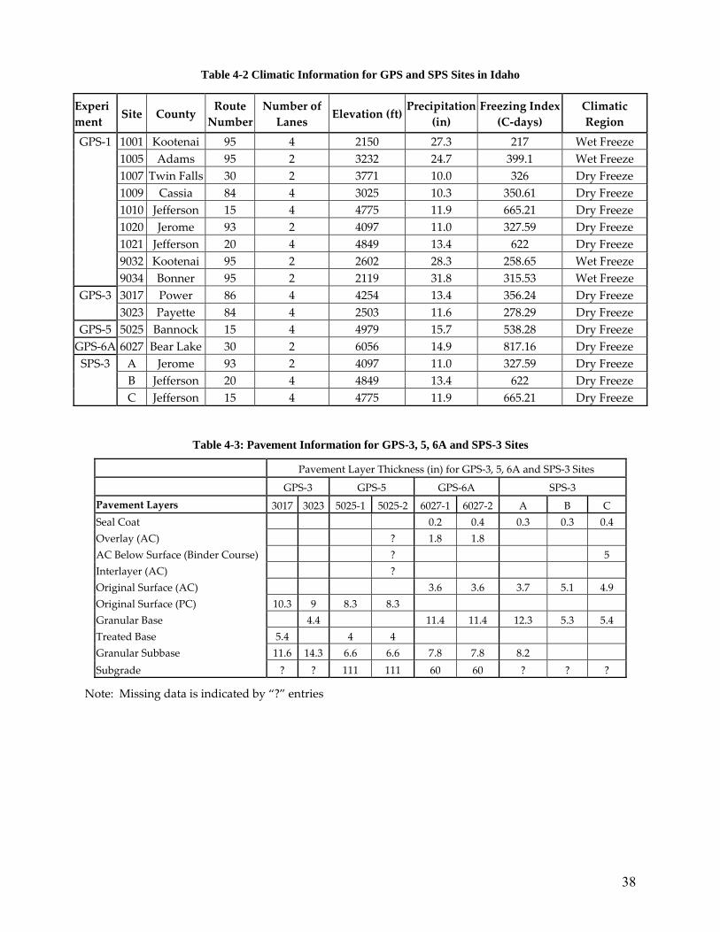
38

Table 4-2 Climatic Information for GPS and SPS Sites in Idaho

Table 4-3: Pavement Information for GPS-3, 5, 6A and SPS-3 Sites

Pavement Layer Thickness (in) for GPS‐3, 5, 6A and SPS‐3 Sites

GPS‐3 GPS‐5 GPS‐6A SPS‐3 Pavement Layers 3017 3023 5025‐1 5025‐2 6027‐1 6027‐2 A B C Seal Coat 0.2 0.4 0.3 0.3 0.4 Overlay (AC) ? 1.8 1.8 AC Below Surface (Binder Course) ? 5 Interlayer (AC) ? Original Surface (AC) 3.6 3.6 3.7 5.1 4.9 Original Surface (PC) 10.3 9 8.3 8.3 Granular Base 4.4 11.4 11.4 12.3 5.3 5.4 Treated Base 5.4 4 4 Granular Subbase 11.6 14.3 6.6 6.6 7.8 7.8 8.2 Subgrade ? ? 111 111 60 60 ? ? ?

Note: Missing data is indicated by “?” entries

Experiment Site County

Route Number

Number of Lanes Elevation (ft)

Precipitation (in)

Freezing Index (C‐days)

Climatic Region

1001 Kootenai 95 4 2150 27.3 217 Wet Freeze 1005 Adams 95 2 3232 24.7 399.1 Wet Freeze 1007 Twin Falls 30 2 3771 10.0 326 Dry Freeze 1009 Cassia 84 4 3025 10.3 350.61 Dry Freeze 1010 Jefferson 15 4 4775 11.9 665.21 Dry Freeze 1020 Jerome 93 2 4097 11.0 327.59 Dry Freeze 1021 Jefferson 20 4 4849 13.4 622 Dry Freeze 9032 Kootenai 95 2 2602 28.3 258.65 Wet Freeze

GPS‐1

9034 Bonner 95 2 2119 31.8 315.53 Wet Freeze 3017 Power 86 4 4254 13.4 356.24 Dry Freeze GPS‐3 3023 Payette 84 4 2503 11.6 278.29 Dry Freeze

GPS‐5 5025 Bannock 15 4 4979 15.7 538.28 Dry Freeze GPS‐6A 6027 Bear Lake 30 2 6056 14.9 817.16 Dry Freeze

A Jerome 93 2 4097 11.0 327.59 Dry Freeze B Jefferson 20 4 4849 13.4 622 Dry Freeze

SPS‐3

C Jefferson 15 4 4775 11.9 665.21 Dry Freeze

39

Table 4-4: Specific Location and Climate Information for Non-Idaho Sites

Experiment State Site Route Number

Functional Class

Number of Lanes

Elevation (ft)

Precipitation (in)

Freezing Index (C‐days)

Climatic Region

GPS‐1 WA 1002 12

Rural Arterial 2 1557 18.7 155.7 Dry Freeze

GPS‐3 WA 3013 195


GPS‐5 OR 5008 84

Rural Interstate 4 2729 17.2 179.8 Dry Freeze

UT 7082 15

Rural Interstate 4 4527 16.7 411.45 Dry Freeze

WA 6056 195


WA 7322 195

Rural Arterial 2 2545 21.1 224.5 Wet Freeze

GPS‐6A

WY 6032 22

Rural Mjr. Collector 2 6156 17.5 894.3 Dry Freeze

Table 4-5: Pavement Information for Non-Idaho Sites

Pavement Layer Thicknesses (in) for Non‐Idaho Sites Pavement Layers OR‐5008 UT‐7082 WA‐1002 WA‐3013 WA‐6056 WA‐7322 WY‐6032

Seal Coat Overlay (AC) 2.5 2.3 2.3 Friction Course 0.3 1.1

Original Surface (AC) 8.1 9.8 4.3 8.2 3.8 4.9 1.9 Original Surface (PC)

AC Below Surface (Binder Course) 2.7 9.8 Interlayer (AC) Granular Base 8 2.2 11.3 9.6 Treated Base 4.4 4.2

Granular Subbase 6 22 36.9 Subgrade ? ? 66 ? ? ? 36

Note: Missing Data is indicated by ?

4.3 METHODOLOGY

Once familiar with the LTPP database, analysis began with the thirteen GPS sites. Data for all

available sites was downloaded for alligator cracking, longitudinal cracking, transverse

cracking and roughness. The data was then extracted and organized by site. For all cracking

data, a sum of the number of cracks per section was used, ignoring the distinction between low,

40

medium or high severity cracks. This was done in an attempt to simplify analysis and also to

eliminate the inconsistency introduced when different data collectors determined the severity

of a specific crack.

For roughness data, an average of the left-wheel and right-wheel path IRI measurements was

used. Each distress parameter was then graphed versus time for each site.

The GPS sites were then grouped according to their corresponding GPS experiment. The

maximum, minimum and average increase rates for each type of distress in a given experiment

group were calculated. These values were analyzed, and thus conclusions based solely on

pavement type were made. Limited analysis was also done on the basis of climate and

temperature by ignoring experiment distinctions and looking at the geographic areas and

functional classes of each roadway.

Similar data for the available SPS sites was also downloaded and organized according to site

and distress type, and eventually grouped by SPS experiment for analysis purposes. Increase

rates were calculated for each site and each distress type both before and after surface

treatment. The changes in increase rates within each SPS experiment were compared to

determine which, if any, surface treatments had a significant impact on improving poor

pavement conditions caused by the various distresses.

4.4 ANALYSIS

The results are organized by experiment type, and include both local and national trends, when

available, for the various distress types. While every attempt was made to complete a thorough

analysis, a lack of local data and national information made it impossible to make consistent

comparisons throughout the report. Very few of the Idaho sites had available data for any of the

cracking types, and all sites providing data were asphalt pavements on granular pavements. In

addition, most of the sites containing cracking data had only one or two data points, making it

inadequate for analysis purposes. Washington, Oregon, Utah, and Wyoming sites also provided

no useful cracking data. Therefore, longitudinal, transverse and fatigue cracking trends could not

be analyzed for GPS sites in Idaho or the surrounding areas. Additionally, national rutting trends

41

were unavailable for GPS-3 and GPS-5 experiments. Consequently, several experiments could

not be compared on a local versus national level for several distresses.

4.4.1 GPS-1: Asphalt Pavements On Granular Bases

The purpose of the GPS-1 experiments is to study the behavior of asphalt pavements on granular

bases with respect to roughness, rutting and fatigue cracking. As described by the LTPP manual,

sections in this experiment include a dense-graded hot mix asphalt concrete (HMAC) surface

layer, with or without other HMAC layers, placed over an untreated granular base. One or more

subbase layers may also be present but are not required. "Full depth" AC pavements are also

included in this study. All GPS-1 distress trends can be found in Appendix B.

4.4.1.1 Analysis of Roughness Data Pavement roughness is quantified using the IRI. Information on gathering roughness data and

computing IRI values can be found in the Data Collection Guide for Long-Term Pavement

Performance Studies (1990).

Roughness Trends in Idaho Of the four experiments in Idaho, asphalt pavements on granular bases showed the most

significant increases in roughness over time, followed by continuous concrete pavements, jointed

concrete pavements, and existing asphalt overlays on asphalt pavements, respectively. The

average increase in roughness with time in the asphalt pavement sites was 0.077 m/km per year,

with increases as high as 0.20 m/km per year in sites 1001 and 1005. The high increases in

roughness in these areas could be attributed to a combination of climate and traffic; both are on

the major arterial US HWY 95 and have a high annual precipitation in comparison to most other

sites (see Error! Reference source not found.), however they also have some of the lower

freezing indices, which is counterintuitive. Figure 4-1 shows the roughness trends for all GPS-1

sites in Idaho.

42

GPS-1 IRI Versus Time

0

0.5

1

1.5

2

2.5

3

Aug-87 May-90 Jan-93 Oct-95 Jul-98 Apr-01 Jan-04 Oct-06

Date

Ave

rage

Rou

ghne

ss (m

/km

)

Site 1001 Site 1005 Site 1007 Site 1009 Site 1010 Site 1020 Site 1021 Site 9032 Site 9034

Figure 4-1: GPS-1 Roughness Trends in Idaho

National Roughness Trends According to FHWA publication FHWA-RD-97-147 (Perera et al, 1998), flexible pavement data

gathered from the LTPP program reveals several trends. In general, pavement roughness

remains relatively constant for the initial years of the pavement life, and after a certain point,

shows a rapid increase in roughness. The average increases in roughness, as gleaned from

figures within the report, are approximately 0.1 m/km per year in dry-freeze regions and 0.05

m/km per year in wet-freeze regions. It is important to note, however, that while the increase

rate for dry-freeze environments is higher than that of wet-freeze environments, the actual

roughness values are higher in the wet-freeze regions. The national trends also show that areas

with high freezing indices or a high number of freeze/thaw cycles had higher roughness values

than those with lower freezing indices.

FHWA publication FHWA-RD-99-193 (Rauhut et al, 1999) presents roughness trends for AC

pavements under both interstate and non-interstate categories. Nearly all sites analyzed under

the non-interstate category showed IRI values less than 2.5 m/km, which is consistent with

roughness values found in Idaho sites. Based on the performance boundaries determined by the

report authors, the majority of sites analyzed feel within the “good” performance range, with IRI

values less than approximately 1.6 m/km. Using the same boundaries, five Idaho GPS-1 sites

43

would fall into the “good” performance category, and all others would be classified as having

“normal” performance.

4.4.1.2 Analysis of Rutting Data Rutting Trends in Idaho Of the four GPS experiments, asphalt pavement on granular bases provided the most useful data

in terms of rutting analysis, as seven of the nine sites could be used. The average increase in rut

depth with time was 0.31 mm per year, with values as high as 0.59 mm per year in section 1001

and as low as 0.00 mm per year in section 1005. The high value for section 1001 can be

explained using the same reasoning as described in the roughness analysis, however the low

value in section 1005 cannot be explained based on this preliminary analysis; climate and traffic

data are similar for both sections 1001 and 1005, and the structural design of the two pavements

is nearly identical as well (see Table 4-1). Figure 4-2 shows the rutting trends for all GPS-1

sites in Idaho.

GPS-1 Rut Depth Versus Time

0

2

4

6

8

10

12

14


Date

Max

imum

Whe

el P

ath

Rut

Dep

th (m

m)

Site 1001 Site 1005 Site 1007 Site 1009 Site 1010 Site 1020 Site 1021 Site 9032 Site 9034

Figure 4-2: GPS-1 Rutting Trends in Idaho

44

National Rutting Trends FHWA publication FHWA-RD-99-193 (Rauhut et al, 1999) presents rutting trends for AC

pavements under both interstate and non-interstate categories. Based on the performance

boundaries presented in the report, nearly all non-interstate sites analyzed fall into the “good” or

“normal” range, with rut depths less than approximately 15mm, depending on pavement age. All

sites in Idaho easily fall into this range, with two sites performing “good” and the remaining

seven having a “normal” performance.

The same publication also analyzed the rutting rate of AC pavements, with approximately 62%

of GPS-1 pavements having a nominal rutting rate (less than 1mm per year). This rate is lower

than the average rutting rate of 0.31 mm per year that was found in Idaho sites. As stated in the

FHWA report, asphalt concrete pavements that are built in wetter, colder climates tend to have a

higher percentage of pavements with poor rutting performance. This correlation provides an

explanation as to the higher rutting rates seen in Idaho versus the national averages.

4.4.1.3 Analysis of Various Cracking Data Cracking Trends in Idaho As stated previously, a lack of usable data within Idaho sites, as well as those in surrounding

states, made analysis of local fatigue, longitudinal and transverse cracking impossible.

National Cracking Trends Longitudinal Cracking National trends for longitudinal cracking in GPS-1 experiments could not be located. Transverse Cracking As discussed in FHWA publication FHWA-RD-99-193 (Rauhut et al, 1999), 64% of sites in

Dry-Freeze climates performed “good” (crack spacing greater than 20 m) while 100% of sites in

Wet-Freeze climates performed “good”. However, no distinction was made between GPS-1 and

GPS-6 pavements in the presentation of these results. Since all sites in Idaho are in one of these

45

two climatic regions, it can be concluded that the majority of asphalt pavements in Idaho are

performing well with respect to transverse cracking.

Fatigue Cracking As discussed in FHWA publication FHWA-RD-99-193 (Rauhut et al, 1999), 94% of sites in

Dry-Freeze climates performed “good” (crack spacing greater than 20 m) while 97% of sites in

Wet-Freeze climates performed “good. However, no distinction was made between GPS-1 and

GPS-6 pavements in the presentation of these results. Since all sites in Idaho are in one of these

two climatic regions, it can be concluded that the majority of asphalt pavements in Idaho are

performing well with respect to fatigue cracking.

4.4.2 GPS-3: Jointed Concrete Pavements

GPS-3 pavement experiments included jointed, unreinforced Portland cement concrete (PCC)

slabs placed over most types of base layers. One or more subbase layers also may have been

present but were not required. The joints may have had either no load transfer devices or smooth

dowel bars. Sampling design factors for this study are moisture, temperature, subgrade type,

traffic rate, dowels, PCC thickness and base type. All GPS-3 distress trends can be found in

Appendix C.

4.4.2.1 Analysis of Roughness Data Pavement roughness is quantified using the International Roughness Index (IRI). Information on

gathering roughness data and computing IRI values can be found in the Data Collection Guide

for Long-Term Pavement Performance Studies (1990).

Roughness Trends in Idaho Jointed concrete pavements showed nearly constant or slight increases in roughness values in

Idaho. Site 3017 showed an increase of approximately 0.045 m/km per year. Figure 4-3 shows

the roughness trends for GPS-3 sites in Idaho.

46


0

0.5

1

1.5

2

2.5


Date

Ave

rage

Rou

ghne

ss (m

/km

)

Site 3017 Site 3023


National Roughness Trends FHWA publication FHWA-RD-98-148 (What Makes….., 2000) presents key findings in the

analysis of roughness trends in PCC pavements. Jointed plain concrete pavements (JPCP) had

higher roughness values in areas with high precipitation and high freezing indices, however

roughness values showed little or no increase over time in wet-freeze regions. In jointed

reinforced concrete pavements (JRCP), roughness values increased with precipitation, subgrade

moisture content, slab thickness, joint spacing and PCC modulus vales. The overall roughness

trend for JRCP pavements appears to increase exponentially. The average increase in roughness

in JRCPs in wet freeze areas was 0.05 m/km per year.

4.4.2.2 Analysis of Rutting Data Rutting Trends in Idaho Jointed concrete pavement experiments in Idaho provided inadequate data for analysis, and only

one site in Washington (53-3013) was found to have applicable values. Thus, the average rate of

increase in rut depth with time for jointed concrete pavements was 0.50 mm per year. Figure 3-1

shows rutting trends for GPS-3 sites in Idaho and Washington.

47


0

2

4

6

8

10

12


Date

Max

imum

Whe

el P

ath

Rut

Dep

th, m

m

Site 3017 Site 3023 WA Site 3013

Figure 4-4: GPS-3 Rutting Trends in Idaho and Washington

National Rutting Trends As described previously, rutting trends were unavailable for GPS-3 sites, and therefore

comparisons between local and national trends could not be made.

4.4.3 GPS-5: Continuous Concrete Pavements

The GPS-5 experiment studies continuously reinforced PCC slabs placed over most types of base

layers. One or more subbase layers may exist but are not required. A seal coat is also

permissible above a granular base layer. All GPS-5 distress trends can be found in Appendix D.

4.4.3.1 Analysis of Roughness Data Pavement roughness is quantified using the IRI and information on gathering roughness data and


Performance Studies (1990) .

48

Roughness Trends in Idaho The single continuous concrete pavement site in Idaho showed nearly constant or slight increases

in roughness values with time. Both before and after the 1996 rehabilitation, roughness values

remained nearly constant with only a slight increase of 0.05 m/km per year prior to maintenance.

Figure 3-1 shows the roughness trend for the single GPS-5 site in Idaho.


0

0.5

1

1.5

2

2.5

3


Date

Ave

rage

Rou

ghne

ss (m

/km

)

Site 5025


National Roughness Trends FHWA publication FHWA-RD-98-148 (What Makes…., 2000) presents key findings in the

analysis of roughness trends in PCC pavements. Continuous reinforced concrete pavements

(CRCP) maintained relatively constant roughness values over time. In wet-freeze locations,

roughness values showed little to no increase over time. In no-freeze areas, higher roughness

values were associated with a higher number of days above 32 degrees Celsius. In all climatic

regions, higher roughness values in CRCPs were associated with higher PCC elastic modulus

values.

49

4.4.3.2 Analysis of Rutting Data Rutting Trends in Idaho Being that there exists only one continuous concrete pavement experiment site in Idaho, two

additional sites were used in Eastern Oregon. However, the data obtained from these two sites

was deemed inadequate for this analysis, thus the single Idaho site was used. This site showed

nearly constant values for rut depth over time, leading to an average increase rate of zero, and

thus having the best performance in terms of rutting. Figure 4-6shows the rutting trends for the

GPS-5 sites in Idaho and Oregon.


0

2

4

6

8

10

12


Date

Max

imum

Whe

el P

ath

Rut

Dep

th, m

m

Site 5025 OR Site 5006 OR Site 5008

Figure 4-6: GPS-5 Rutting Trends in Idaho and Oregon

National Rutting Trends As described previously, rutting trends were unavailable for GPS-5 sites, and therefore

comparisons between local and national trends could not be made.

50

4.4.4 GPS-6A: Existing Asphalt Overlays on Asphalt Pavements

The GPS-6 experiments include pavement sections, which were a part of the original LTPP

experimental design for rehabilitated pavements, as well as those that have been added in

response to changes in practice. Pavements included for GPS-6A, Existing AC Overlay of AC,

have a dense-graded HMAC surface layer with or without other HMAC layers placed over a

previously existing AC pavement. The total thickness of HMAC used in the overlay is at least 25

mm (1.0 inch). All GPS-6A distress trends can be found in Appendix E.

4.4.4.1 Analysis of Roughness Data Pavement roughness is quantified using IRI and information on gathering roughness data and


Performance Studies (1990).

Roughness Trends in Idaho The sole GPS-6 site in Idaho showed nearly constant roughness values for all data points, with a

maximum IRI value of 1.62 m/km and a maximum roughness increase rate of 0.20 m/km per

year. Figure 4-7 shows the roughness trend for the single GPS-6A site in Idaho.

National Roughness Trends As presented in FHWA publication FHWA-RD-00-165 (Performance Trends…., 2000), nearly

one quarter of the GPS-6 test sections showed roughness values greater than the nominal level of

roughness selected for this study (less than 1.6 m/km). No correlations between climatic data

and roughness values, or roughness values over time were presented. However, it is noted that

the amount of traffic on an overlay significantly affects the rate of increase of roughness, while

the initial condition of the pavement (prior to rehabilitation) has little to do with the overlay

roughness.

FHWA publication FHWA-RD-99-193 (Rauhut et al, 1999) presents national trends for GPS-6A

sites with respect to roughness. All but two data points fall within the “normal” or “good”

performance range, which, as determined by the report authors, is approximately less than 3.18

51

m/km, depending on pavement age. The sole Idaho GPS-6A site falls within the “good” range of

this study’s boundary selection.


0

0.2

0.4

0.6

0.8

1

1.2

1.4

1.6

1.8

Dec-88 May-90 Sep-91 Jan-93 Jun-94 Oct-95 Mar-97

Date

Ave

rage

Rou

ghne

ss (m

/km

)

Site 6027

Figure 4-7: GPS-6A Roughness Trends in Idaho

4.4.4.2 Analysis of Rutting Data Rutting Trends in Idaho The sole existing asphalt overlay on asphalt pavement site in Idaho also provided data that was

not applicable; however one site in Wyoming (56-6032) and two sites in Washington (53-6056,

53-7322) were found to have adequate data. The average rate of increase in rut depth was 0.42

mm per year for these experiments. Figure 4-8 shows the rutting trends for GPS-6A sites in

Idaho, Washington and Wyoming.

52

GPS-6A Rut Depth Versus Time

0

2

4

6

8

10

12

Aug-87 May-90 Jan-93 Oct-95 Jul-98 Apr-01 Jan-04

Date

Max

imum

Whe

el P

ath

Rut

Dep

th, m

m

Site 6027 WA Site 6056 WA Site 7322 WY Site 6029 WY Site 6032

Figure 4-8: GPS-6A Rutting Trends in Idaho, Washington and Wyoming

National Rutting Trends As presented in FHWA publication FHWA-RD-00-165 (Performance Trends …., 2000), one

third of the GPS-6 test sections had rut depths greater than 7 mm. Again, no correlations

between climatic data and rut depth, or rut depth over time were presented. The analysis shows

that thick overlays do no resist rutting any more than thin overlays. It is noted that material

properties and construction techniques are likely to be the most important factors in the severity

of rutting.

FHWA publication FHWA-RD-99-193 (Rauhut et al, 1999) also presents national trends for

GPS-6A sites with respect to rutting. The majority of analyzed data points fall into the “normal”

or “good” performance range, which, as determined by the report authors, is approximately less

than 10 mm, depending on pavement age. The sole Idaho GPS-6A Idaho site, as well as those

sites in surrounding states, also falls within this “normal” or “good” range. Also presented in

this report was the rutting rate of GPS-6A pavements. 49% of GPS-6A pavements showed a

nominal rutting rate (less than 1 mm per year) while 13% showed a moderate rutting rate

53

(between 1 and 2 mm per year). Based on these rutting rate distinctions, the Idaho and

surrounding area GPS-6A sites easily qualify as having nominal rutting rates, as their average

rate of increase in rut depth was 0.42 mm per year.

4.4.4.3 Analysis of Various Cracking Data Cracking Trends in Idaho As stated previously, a lack of usable data within Idaho sites, as well as those in surrounding

states, made analysis of fatigue, longitudinal and transverse cracking impossible.

National Cracking Trends Longitudinal Cracking As presented in FHWA publication FHWA-RD-00-165 (Performance Trends…., 2000),

approximately twenty percent of the GPS-6 test sections contained more than 50 meters of

longitudinal cracking, both in and out of the wheel path. Again, no correlations between climatic

data and longitudinal cracking, or longitudinal cracking over time were presented. Neither the

condition of the pavement prior to rehabilitation nor the age of the overlay has a significant

impact on its performance with respect to longitudinal cracking.

Transverse Cracking As presented in FHWA publication FHWA-RD-00-165 (Performance Trends…, 2000), thirty-

five percent of the GPS-6 test sections have more than eleven transverse cracks. Again, no

correlations between climatic data and transverse cracking, or transverse cracking over time were

presented. However, it is noted that while transverse cracks are believed to be caused by low

temperatures, only moderate to low amounts of transverse cracks were observed in Canadian test

sections, where low temperatures are common. Unlike longitudinal cracking, the original

pavement condition prior to overlay placement does affect the amount of cracking observed in

the overlay. The age of the overlay affected its performance with respect to transverse cracking

in thin overlays (less than 60 mm) but not in thicker overlays. Also, as the thickness of an

overlay increases, so does its resistance to transverse cracking.

54

FHWA publication FHWA-RD-99-193 (Rauhut et al, 1999) presents national transverse

cracking trends for all AC pavements, but does not distinguish between GPS-1 and GPS-6

pavements. See previous sections for a summary of these trends.

Fatigue Cracking As presented in FHWA publication FHWA-RD-00-165 (Performance Trends…., 2000), fifteen

percent of the GPS-6 test sections have more than 11 m2 of fatigue cracking. Again, no

correlations between climatic data and fatigue cracking, or fatigue cracking over time were

presented. However, a correlation between longitudinal cracking in the wheel path and fatigue

rutting was made. It was found that with continued traffic loading, longitudinal cracking in the

wheel path will evolve into fatigue cracking.

FHWA publication FHWA-RD-99-193 (Rauhut et al, 1999) presents national fatigue cracking

trends for all AC pavements, but does not distinguish between GPS-1 and GPS-6 pavements.

See previous sections for a summary of these trends.

4.4.5 SPS-3: Pavement Treatment Performance

SPS-3 compares the effectiveness and mechanisms by which the selected maintenance

treatments preserve and extend pavement service life, safety and ride quality. The overall goal

was not to compare the performance of one treatment to another, but to compare the change in

performance of the treated section to the untreated section. The study factors for flexible

pavements include: climatic zone, subgrade type (fine or coarse), traffic loading (greater or less

than 85,000 ESALs/year), initial condition (good, fair, or poor), and structural adequacy (high or

low). The maintenance treatments applied were slurry seal, chip seal, crack seal and thin overlay.

All SPS distress trends can be found in Appendix F.

Three SPS-3 experiments were conducted in Idaho (SPS3-A, B and C). The results of the

analysis of various treatment performances for each distress type are discussed below. National

performance trends were gleaned from the FHWA publication FHWA-RD-96-208 (Morian et al,

1997).

55

4.4.5.1 Thin Overlay Treatment Treatment Performance in Idaho Roughness The thin overlay treatment performed the best, with regards to roughness, in sections SPS3-A

and B. SPS3-C also showed a marked improvement in roughness after the application of a thin

overlay.

Rutting The application of a thin overlay seemed to have little or no effect on resisting rutting in the three

Idaho SPS-3 experiment sites.

Longitudinal Cracking The only test sections using a thin overlay treatment recorded zero longitudinal cracks prior to

treatment. Therefore, no analysis could be conducted on its performance in treating this distress.

Transverse Cracking The single SPS site providing transverse cracking data for thin overlay treatments showed no

improvement in pavement condition after treatment.

Fatigue Cracking The only test sections using a thin overlay treatment recorded zero fatigue cracking prior to


Treatment Performance Nationally In all regions, the thin overlay treatments performed the best after five years.

4.4.5.2 Slurry Seal Treatment Treatment Performance in Idaho Roughness In section SPS3-C, the slurry seal treatment performed best in improving the roughness of the

pavement. A slight improvement in roughness was noted in SPS3-A and B due to the

application of the slurry seal coat.

56

Rutting The application of a slurry seal coat performed the best at resisting rutting of all treatments in

section SPS3-B. No significant improvement in rutting from this treatment was noted at the

other test sections

Longitudinal Cracking Only one test section using the slurry seal treatment also recorded longitudinal cracking data.

From this data, it was concluded that the slurry seal coat provided an initial improvement by

reducing the number of cracks; however, within a few years, the same number of longitudinal

cracks as was observed prior to treatment reappeared.

Transverse Cracking The single SPS site providing transverse cracking data for slurry seal treatments showed no


Fatigue Cracking The only test sections using a slurry seal treatment recorded zero fatigue cracking prior to


Treatment Performance Nationally The slurry seal treatments were also best in the Southern Region, but performed very poorly in

the North Central Region.

4.4.5.3 Crack Seal Treatment Treatment Performance in Idaho Roughness The application of a crack seal coat had no effect on roughness in any of the three Idaho test

sections.

Rutting The application of a crack seal coat showed a slight improvement in rutting in section SPS3-B.

No significant improvement in rutting from this treatment was noted at the other test sections.

Longitudinal Cracking No test sections using a crack seal treatment provided longitudinal cracking data. Therefore, no

analysis could be made on its performance in treating this distress.

57

Transverse Cracking The single SPS site providing transverse cracking data for crack seal treatments showed no


Fatigue Cracking The only test sections using a crack seal treatment recorded zero fatigue cracking prior to


Treatment Performance Nationally Crack seals performed very well in the North Atlantic and North Central Regions, but were

unsuccessful in the Western and Southern Regions

4.4.5.4 Chip Seal Treatment Treatment Performance in Idaho Roughness The application of a chip seal coat had no effect on roughness in any of the three Idaho test

sections.

Rutting The application of a chip seal coat showed no significant improvement in rutting in any of the

three Idaho test sections.

Longitudinal Cracking The only test sections using a chip seal treatment recorded zero longitudinal cracks prior to


Transverse Cracking Two sections, SPS3-B and C, provided transverse cracking data for chip seal treated pavements.

Both sections showed no improvement in transverse cracks due to this treatment.

Fatigue Cracking No test sections using a chip seal treatment provided fatigue cracking data. Therefore, no

analysis could be made on its performance in treating this distress.

58

Treatment Performance Nationally Chip seals performed fairly well, although they performed best in the Southern Region.

4.5 CONCLUSIONS FORM IDAHO SITES

4.5.1 GPS Sites

Since cracking trends were not considered for GPS sites in Idaho, conclusions as to the most

effective pavement type is based solely on its performance with regards to roughness and rutting.

Continuous concrete pavements performed best in both areas, while jointed concrete pavements,

asphalt pavements on granular bases and existing asphalt overlays on asphalt pavements had

mediocre performances.

4.5.2 SPS Sites

With regards to cracking and rutting, the surface treatments tested were not effective at

improving pavement conditions. To improve pavement roughness, a thin overlay is the best

treatment option, followed by the placement of a slurry seal coat. Chip and crack seal

treatments again have no impact on pavement roughness.

59

5. SEASONAL VARIATION OF SUBGRADE RESILIENT MODULUS – NATIONAL LTPP DATA

5.1 INTRODUCTION

As mentioned earlier, there was only one seasonal site in Idaho, and therefore, data from other

LTPP seasonal sites (form allover the national sites) were used to investigate the variability of

the subgarde resilient modulus with seasonal variation. This investigation was published in a

paper at the TRB annual meting by Salem and Bayomy (2003). The goal of the research was to

develop regression models that can enable design engineers to assess the seasonal changes in the

resilient modulus, and to develop an algorithm for calculating a seasonal adjustment factor that

allows estimating the subgrade modulus at any season from a known reference value at a given

season.

5.2 BACKGORUND ON THE LTPP SMP STUDY

The FHWA-LTPP team launched the Seasonal Monitoring Program (SMP) as an integral part of

the LTPP program. The primary objective of the SMP was to study the impacts of temporal

variations in pavement response and materials properties due to the separate and combined

effects of temperature, moisture and frost/thaw variations. The SMP experiment focused on

collecting data that capture the seasonal variations of the pavement material properties along

with the associated variations in pavement performance. The factorial design of the SMP

experiment included 32 different study factors. Table 5-1 summarizes the original experiment

design of the LTPP-SMP. The original design included 32 design cells, with three sites to be

selected for each flexible pavements cell (cells 1-16) and one site for each rigid pavement

cell(cells 17-32). However, and due to practical implementation of this huge study program, not

all cells were filled with the required number of sites. The data collected by the FHWA-LTPP

program for the SMP study included, in addition to the basic LTPP data designated for the

General Pavement Studies (GPS), data that relate to the seasonal variations of the material

properties and the structural capacity of the exiting pavements. The data types that were

collected under the SMP study are listed in Table 5-1. Most of the LTPP data were released to

60

the public in CD formats via the DataPave software. The latest DataPave software released is

version 3.0, which includes the data release in January 2002.

The approach adopted in this study was to select LTPP-SMP sites that represent various soil

categories and use the backcalculated modulus and gravimetric moisture content data in the

LTPP database to develop regression models for the modulus-moisture relationships for various

soils.

Table 5-1: Experimental Design and Data Elements for the LTPP Seasonal Monitoring Program (Rada et al, 1994)

a) LTPP-SMP Experimental Design

No Freeze Zone Freeze Zone Pavement Type Subgrade

Soil Type Dry Wet Dry Wet

Fine 1 2 3 4 Flexible, Thin AC Surface, <127 mm Coarse 5 6 7 8

Fine 9 10 11 12 Flexible, Thick AC Surface, >127 mm Coarse 13 14 15 16

Fine 17 18 19 20 Rigid –Jointed Plain Concrete, JPC Coarse 21 22 23 24

Fine 25 26 27 28 Rigid Jointed Reinforced Concrete, JRC Coarse 29 30 31 32

b) SMP Data Elements

Element Type of Data Collected

Structural Capacity Deflection data using FWD

Environmental Related Data

Ambient Temperature and rainfall Pavement surface and air temperature Surface layer temperature profile Moisture – depth profile Depth of frost /thaw Depth of ground water table Joint opening and joint faulting (rigid pavements)

Elevation and Profile Data Surface elevation (rod and level) Longitudinal profile (profiler/dipstick)

Distress Data Distresses (Photographic /annual)

61

5.3 MODULUS-MOISTURE RELATIONSHIP FOR SUBGRADE SOILS

The relationship between the modulus of resilience of the soil and its changes with moisture has

been studied for many decades. Most of the published information is based on laboratory or

small-scale field experiments. A brief summary of previous work discussing the effect of

seasonal variations on the soil resilient modulus is presented in the following subsections.

5.3.1 Moisture Effects on Soil Resilient Modulus

Many researchers have investigated the influence of water content on the resilient modulus of

fine-grained soils. Seed et al, (1962) studied the influence of "natural" water content on the

resilient modulus of undisturbed samples of the silty clay subgrade soil used in the AASHO

Road Test. The positions of the test points showed that for this soil a decrease in water content

of only three percent below the optimum resulted in a doubling of the resilient modulus. For

instance, the data showed a modulus increase from about 34 MPa to about 69 MPa upon

decrease in moisture of 3% (Seed et al, 1962).

Tests conducted on silty clay subgrade soil at the San Diego County Experimental Base Project

by Jones and Witczak (1977) showed that as its compaction water content was increased from

about 11 percent to about 20 percent the resilient modulus varied from almost 275 MPa to as low

as about 52 MPa.

Carmichael and Stuart (1985) presented correlations relating the resilient modulus to

fine-grained soil composition parameters. Using a database representing over 250 soils (fine and

coarse) and 3,300 modulus test data points, they developed the following relationship:

Mr = 37.431 - 0.4566 PI - 0.6179 w - 0. 1424F + 0.1791CS - 0.3248 σd + 36.422CH + 17.097

MH (2)

62

Where Mr is the resilient modulus in ksi, PI is plasticity index in percent, w is the water content

in percent, F is percent passing sieve No. 200, CS is the confining stress in psi and σd is deviator

stress in psi. The CH term is a material factor which is equal to one for soils classified as CH and

is equal to zero for soils classified as ML, MH, or CL. MH is a material factor equal to one for

soils classified as MH and equal to zero for soils classified as ML, CL, or CH.

The moisture sensitivity of coarse-grained materials depends on the amount and nature of its fine

fraction. Clean gravels and sands classified as GW, GP, SW, and SP are not likely to exhibit

moisture sensitivity due to the absence of a sufficient number of the small pores necessary to

create significant suction-induced effective stresses even at low water contents (Hicks and

Monismith, 1971). Studies of coarse materials containing larger amounts of fines have shown

that increasing degrees of saturation above 80 to 85 percent can have a pronounced effect on

resilient modulus. Rada and Witczak (1981) concluded that changes in water content of

compacted aggregates and coarse soils could cause modulus decreases of up to 207 MPa.

Several researchers have developed regression relationships between the resilient modulus of

granular materials and water content. The general regression relationship for granular materials

of Carmichael and Stewart (1985), stated previously as Equation 2, contains a water content term

that results in a 0.62 Ksi (4.3 MPa) decrease in resilient modulus for each one percent increase in

water content. Lary and Mahoney (1984) found regression relationships for resilient moduli of

specific northwest aggregate base materials and predominantly coarse subgrade soils. The

regression equations for the materials showed that if the initial modulus is on the order of 140

MPa, a one percent increase in moisture content typically results in a resilient modulus decrease

from about 4 to 11 MPa. A reasonable estimate for the influence of water content on reference

resilient modulus of coarse soils would be about 3.4 MPa decrease for each one percent moisture

content increase for uniform or well-graded coarse materials containing little or non-plastic fines

(GW, GP, SW, SP). That value would increase to about 3.8 MPa per one percent moisture

content increase for sands and gravels containing substantial amounts of plastic fines (GM, GC,

SM, SC).

63

For the development of AASHTO2002, Witczak et al (2000) developed the model shown below

by Eqn. 3 for evaluating the change in modulus of resilience due to change in moisture content.

Log {Mr / Mr-opt} = a + (b-a) / (1+ exp(c + d (S-Sopt))) (3)

Where;

Mr = Resilient modulus at any degree of saturation, S

Mr-opt = Resilient modulus at optimum moisture content

S = Degree of saturation in decimal.

Sopt = S at optimum

a, b, c, d = Model parameters

5.3.2 Temperature Effects on Subgrade Soil Resilient Modulus

Low temperatures, below freezing, may cause significant variation of the soil moduli values. The

penetration of freezing temperatures into moist soils may cause the moisture in the soil voids to

freeze. The soil-moisture system during the freezing condition will show much higher modulus

value. However, during the thaw period, the material loses the apparent increase in its modulus.

This effect is more profound in soft soils, where the material softens further in the thaw season

and it loses its strength significantly below its normal value. Study by Hardcastle (1992) showed

that freezing of soil moisture could transform a soft subgrade into a rigid material. However,

thawing of the same material can produce a softening effect such that for some time after

thawing, the material would have a resilient modulus that is only a fraction of its pre-freezing

value. The effects of an annual cycle of freezing and thawing on the deflections of pavements

having coarse and fine-grained subgrade soils in Illinois and Minnesota were studied by Scrivner

et al. (1969). The study showed that, for all of the pavements, freezing results in sharp reductions

in surface deflections while thawing produces immediate deflection increase. It showed also that

the pavement deflection changes could occur due to freezing of the structural layers alone, while

the largest thaw-induced deflection increases take place when there is deep frost penetration into

the fine-grained subgrade soils. Deflection increases due to deep frost penetration and thawing of

the coarse-grained subgrade soil are smaller than those for fine-grained soils.

64

5.3.3 Subgrade Moisture Prediction Using the Integrated Climatic Model (ICM)

Recent studies are showing that important climatic factors such as temperature, rainfall, wind

speed and solar radiation can be modeled accurately enough for design purposes by using a

combination of deterministic and stochastic analytical methods. These techniques provide the

input into climatic-materials-structural-infiltration-drainage frost-penetration frost-heave and

thaw weakening models that result in meaningful simulations of the behavior of pavement

materials and of subgrade conditions or characteristics over several years of operation. The

Integrated Climatic Model developed under contract to Federal Highway Administration by

Lytton et al. (1989) has been designed to perform these tasks. Larson and Dempsey (1997-2000)

upgraded the model for the ICM version 2.1. It could be applied to either asphalt or Portland

cement concrete pavements. The model is composed of four major components. They are the

Precipitation (PRECIP) Model, the Infiltration and Drainage (ID) Model, the Climatic-Material-

Structural Model (CMS) Model and the CRREL (The U.S. Army Cold Regions Research and

Engineering Laboratory) Model for Frost Heave-Thaw Settlement. For the development of

AASHTO2002, the NCHRP 1-37(a) research team modified the ICM and developed the

enhanced ICM. The new version of the model is called EICM 2.62 (Witzak et al, 2000).

Richter and Witczak (2001) have discussed the application of data collected at 10 LTPP SMP

sites to evaluate the volumetric moisture prediction capabilities of the ICM. The moisture

prediction capabilities of the Integrated Climatic Model (ICM) were evaluated by applying the

model to predict the subsurface moisture contents for the test sections, and then comparing the

results to the data collected at those sites. Several versions of the ICM model were considered in

this work. Six of the sites were modeled with Version 2.1 of the ICM. Poor agreement between

the model output and the monitored moisture data was observed because several of the key

material parameters required by the model are not among the data collected for the test sections

used in the evaluation. Based on their findings, Richter and Witczak (2001) concluded that

Version 2.62 of the ICM could sometimes provide reasonable estimates of the variation in the in-

situ moisture content of unbound pavement materials. The findings for one of the sites suggested

that the model might not work well for sites in arid climates; however, they recommended more

extensive evaluation to draw definitive conclusions in this regard.

65

5.3.4 Seasonal Variation and Seasonal Adjustment Factors

In a study on the LTPP data by Ali and Parker (1996), they found out that the backcalculated

resilient moduli of both subgrade and AC surface could be correlated to the month of the year in

a sinusoidal function with reasonable accuracy.

Several research projects were conducted at the University of Idaho by Hardcastle (1992), Al-

Kandari (1994), Bayomy et al (1977), studying the effect of seasonal variations on pavement

performance). These research projects provided initial values of subgrade soil resilient modulus

for various climatic regions and soil types across the State of Idaho. Based on these studies,

Bayomy et al (1996) developed seasonal adjustment factors (SAF) for subgrade soils in Idaho

and incorporated them in the Idaho overlay design system, WINFLEX 2000 (Bayomy and Abo-

Hashema, 2001).

The Washington State Department of Transportation (WSDOT) uses a mechanistic-empirical

system developed at the University of Washington and implemented in the computer program

EVERPAVE 5.0 (Sivaneswaran et al, 1999). This program uses the SAF as key inputs by users

and it does not compute the SAF.

The Minnesota Department of Transportation (Mn/DOT) uses a mechanistic-empirical (M-E)

flexible pavement thickness design that is implemented in the computer program ROADENT 4.0

by Timm et al (2001). The ROADENT program does not include the SAF to adjust the resilient

modulus from one season to another; therefore the user has to calculate and enter the resilient

modulus values for each season.

The above studies demonstrate that there is need to establish realistic prediction models that

allow the prediction of the subgrade soil modulus at various seasons. The prediction can be in the

form of a direct relationship between the modulus and the moisture at a selected season, or in the

form of a seasonal adjustment factor (SAF) that shifts the modulus value from a known reference

modulus to that of the season in consideration.

66

5.4 LTPP-SMP DATA REQUISITION AND PREPARATION

The first step in the analysis was to isolate all sites in the freeze zones (wet and dry) from the

non-freeze zones since the frost susceptibility of a soil would certainly influence its modulus

change, especially in the transition from the freeze period to the thaw period. It is also

recognized that the frost susceptibility issue is another main factor that may influence soil

behavior in the freeze and thaw period. It was decided that this chapter would concentrate on

moisture variation effects in “non-freeze” zones.

Next, extensive data mining was performed to gather and consolidate available data in all sites in

the no-freeze zones (wet or dry), which have sufficient data that allows the development of the

desired prediction models. The extensive analysis revealed seven LTPP sites that were used in

the analysis. Table 5-2 presents the selected sites, and the subgrade soil properties at these sites.

It is important to note that even though the LTPP site number 24-1634 is located in Maryland,

which is classified geographically as Freeze zone, the climatic data of this site indicated no frost

conditions but the authors included the data obtained from this site in their analysis because it

was the only site that had fine silt subgrade soil.

The downloaded data for each site included the backcalculated elastic moduli for subgrade soil

and asphalt concrete (AC) surfaces, the AC layer temperature, and both volumetric and

gravimetric moisture content of subgrade soil at different time intervals. The Backcalculated

subgrade resilient (elastic) modulus was obtained from the LTPP database table

(MON_DEF_FLX_BAKCAL_SECT). The gravimetric moisture content was obtained from the

table SMP_TDR_AUTO_MOISTURE. These tables are available in the DataPave software. For

the purpose of this study, only the analyses of the change in subgrade soil moduli with seasonal

moisture variation were considered. The moisture content of the subgrade is provided in the

LTPP database as moisture profile along the subgrade depth. The average moisture content along

the depth was considered the corresponding moisture for the backcalculated resilient modulus at

a given location.

67

Table 5-2: Selected LTPP Sites and Subgrade Soil Characterizations

1 2 3 4 5 6 7 LTPP Sites

48-4143 13-1005 48-1122 24-1634 48-1077 35-1112 28-1016

Location Texas (TX)

Georgia (GA)

Texas (TX)

Maryland (MD)

Texas (TX)

New Mexico (NM)

Mississippi (MS)

Surface Type Rigid Flexible Flexible Flexible Flexible Flexible FlexibleMinimum Monthly Avg. Air Temp, Co

9.7 8.7 9.7 1.7 3.6 5.8 5

Soil Type as Identified by the LTPP

Lean Inorganic Clay

Fine Clayey Sand

Coarse Clayey Sand

Fine Silt Fine Sandy Silt

Coarse, poorly graded sand

Coarse, Silty sand

AASHTO Soil Classification A-7-6 A-6 A-2-6 A-4 A-4 A-3 A-2-4

% Passing # 4 - - 99 99 94 100 92 % Passing # 10 - - 97 98 93 99 91 % Passing # 40 - - 75 98 87 94 85 % Passing # 200 90 38.4 6.5 97.9 51.8 2.7 25.7

D60, mm - - 0.3 - 0.1 0.18 0.23 Liquid Limit, % 41 27 26 - - - 18

Plasticity Index, % 23 12 12 NP NP NP 3

Max. Dry Density, gm/cm3

1.730 2.05 1.858 1.746 1.906 1.698 1.906

Optimum Moisture, % 15.0 10.0 8.0 12.0 10.0 12.0 13.0

5.5 DATA ANALYSIS

The selected sites were placed in two groups, sites for plastic soils (LTPP sites 48-4143, 13-

1005, and 48-1122), and non-plastic subgrade soil (LTPP sites 24-1634, 48-1077, 35-1112 and

28-1016). In the following discussions, the sites will be referred to by their serial numbers (1

through 7), shown in Table 3-1. The data were analyzed to investigate the changes over time

68

(time series analysis), and to develop models for modulus prediction for both types of soil

groups. In addition, a generalized model for seasonal adjustment factor was developed.

5.5.1 Moisture and Modulus Variation with Time

Time series plots for the relationship between both gravimetric moisture content and subgrade

backcalculated modulus for the different sites considered in this study are presented in 26.

The data indicate that both moisture content and backcalculated elastic modulus have almost a

sinusoidal function with time. The data also indicate that the backcalculated elastic modulus

could be related to moisture content in an inverse function. It increases when the moisture

decreases, and vice versa. This correlates with the data obtained by Ali and Parker (1996). The

same behavior is observed at all sites except for site 28-1016, where the modulus showed an

increasing function with increasing moisture content. Careful analysis of the data showed that the

subgrade soils at that site had recorded field moisture contents that were below the lab optimum

moisture content. Since the soil is granular (coarse silty sand) and has very low plasticity (PI=3),

it is most likely that the field condition was on the dry side of the optimum, which may lead to an

increase in the modulus with the increase in moisture content until near the optimum. The results

for sites 24-1634 and 13-1005 in Figure 5-1 indicates that the maximum modulus values and

minimum moisture values are measured through the summer season (July and August), while the

minimum modulus values and maximum moisture values are measured through the winter

(January and February).

5.5.2 Model Development for Plastic Soils

Multiple regression analysis techniques were applied to relate the backcalculated elastic modulus

to subgrade moisture content and other soil properties such as Atterberge limits and percentage

passing sieve # 200. Data from the first three LTPP sites (48-4143,13-1005 and 48-1122) were

used in this analysis. The subgrade soils at these three sites are: clay, fine sandy clay and coarse

sandy clay, respectively.

Based on study by Carmichael and Stuart (1985), a model that includes the fine content and the

plasticity index as representative of the soil properties was suggested. After intensive statistical

analysis, the best form of the relationship between the soil resilient modulus and other related

soil parameters was chosen in the form:

69

Figure 5-1: Variation of Modulus and Moisture with Time for Various Soil Types at the Selected

LTPP Sites.

70

E1 = Co + C1 * X1 + C2*X2 + C3 * F + C4* PI (4)

Where;

E1 = Log (E)

E = Backcalculated elastic modulus, MPa

X1 = log (moisture content, %) X2 = 1/ (moisture content, %)

F = Percentage passing sieve # 200, %

PI = Plasticity index, %

Co, C1, C2, C3 and C4 are regression coefficients.

The Statistical Analysis System (SAS Software, 2001) computer program was used to perform

the multiple regression analysis with the model proposed by Equation 4 above. The program’s

output of the regression analysis is shown in Table 5-3. The ANOVA results indicate that the

logarithm of the backcalculated modulus (E1) could be related only to the logarithm of moisture

content (X1), with a function having a coefficient of determination (R2) value of 0.6981.

However, when adding other soil properties like PI and F to the model, a better model having R-

square value of 0.9891 could be achieved. Hence, a regression model in the form of Equation 4

was fitted. The results of the regression analysis for the model are also shown in Table 5-3. The

results of the statistical test that evaluates the significance of each regression coefficient indicate

that the estimated model parameters are significant (p-value is less than 0.05). The final model

for this group of soils, based on 183 data points, is represented by Equation 5 below:

Log (E) = 8.82 – 0.673 * X1 – 2.44 * X2 + 0.0084 * F – 0.11* PI (5)

Error! Reference source not found.Figure 5-2 shows the model application on the data

collected from sites 48-4143,13-1005 and 48-1122, respectively. The three plots in the figure

indicate that the model fits the data very well and that the modulus decreases with increasing soil

moisture even if the field moisture content is less than the optimum moisture content, as in sites

13-1005 and 48-1122, respectively. This would be acceptable since the subgrade soils at both

sites are cohesive soils (sandy clay). Hence, when the moisture content decreases, the soil

becomes harder and its modulus increases, and vice versa. It should be noted that this model

71

could be applied only for plastic soils, as there is a term in the model for PI. For non-plastic soils,

this model will be modified to account for soil properties other than PI, as is discussed below.

Table 5-3: SAS Output for Regression Analyses for Modulus-Moisture Relationship for Plastic Soils The REG Procedure Model: MODEL1 Dependent Variable: E1 R-Square Selection Method Number in Root Model R-Square C(p) BIC MSE Variables in Model 1 0.9767 176.6577 -844.4975 0.07112 PI 1 0.7840 2926.776 -491.2373 0.21651 F 1 0.6981 4151.479 -437.8291 0.25593 x1 1 0.5068 6880.904 -359.4122 0.32712 x2 ------------------------------------------------------------------------------- 2 0.9795 137.8704 -863.9304 0.06683 F PI 2 0.9768 177.2805 -844.1832 0.07120 x2 PI 2 0.9767 178.3979 -843.6575 0.07132 x1 PI 2 0.9022 1241.671 -617.3199 0.14614 x1 x2 ------------------------------------------------------------------------------- 3 0.9884 13.2697 -950.0654 0.05045 x1 F PI 3 0.9871 32.4110 -933.3682 0.05329 x2 F PI 3 0.9781 159.8558 -852.5841 0.06930 x1 x2 PI 3 0.9161 1045.302 -641.4009 0.13579 x1 x2 F ------------------------------------------------------------------------------- 4 0.9891 5.0000 -957.7523 0.04902 x1 x2 F PI

The REG Procedure Model: MODEL1 Dependent Variable: E1 Analysis of Variance Sum of Mean Source DF Squares Square F Value Pr > F Model 4 33.90986 8.47747 3528.46 <.0001 Error 155 0.37240 0.00240 Corrected Total 159 34.28227 Root MSE 0.04902 R-Square 0.9891 Dependent Mean 5.70630 Adj R-Sq 0.9889 Coeff Var 0.85899 Parameter Estimates Parameter Standard Variance Variable DF Estimate Error t Value Pr > |t| Inflation Intercept 1 8.81933 0.31794 27.74 <.0001 0 x1 1 -0.67276 0.12405 -5.42 <.0001 301.27894 x2 1 -2.43912 0.76112 -3.20 0.0016 135.24219 F 1 0.00838 0.00066926 12.52 <.0001 32.88774 PI 1 -0.11065 0.00343 -32.28 <.0001 16.50651

Summary of Regression Coefficients (Model presented by Equation 4):

C0 = 8.81933 C1 = -0.67276 C2 = -2.43912 C3 = 0.00838 C4 = -0.11065

72

Clayey Soil, Site 48-4143100

105

110

115

120

125

130

135

140

20 20.5 21 21.5 22 22.5 23 23.5

Mois ture Content, %

Mod

ulus

, MP

Collected DataModel

Fine Sandy Clay, Site 13-1005

350

370

390

410

430

450

470

7.0 8.0 9.0 10.0 11.0 12.0 13.0 14.0Mois ture Content, %

Mod

ulus

, MP

a

Collected DataModel

290

310

330

350

370

390

410

430

450

3.0 4.0 5.0 6.0 7.0 8.0 9.0 10.0

Mois ture Content, %

Mod

ulus

, MP

a

Collec ted DataModel

Coarse Sandy Clay , Site 48-1122

Figure 5-2: Model Development for Non-Plastic Soils

73

As was described previously, the model shown in Equation 5 could not be applied directly for

non- plastic soils (sandy and/or silty soils), since there is a term in the model for PI. However, a

general model in the form of equation 3 can be used after replacing the PI variable with the soil

parameter D60, which is the soil size for 60% passing. This was selected based on the study by

Witczak et. al (2000).

Similar to the above analysis on plastic soils, data from sites (24-1634, 48-1077 and 35-1112)

with non-plastic materials were used to develop a model in the form:

E1 = Co + C1 * X1 + C2*X2 + C3 * F + C4* D60 (6)

Where variables E1, X1, X2 and are defined as in equation 3, and D60 is the soil grain size for 60% passing.

SAS results revealed that the C1 coefficient was insignificant. Then the model was modified to

exclude the term X1 (Log (Moisture content), and the regression was conducted on the model

with three independent parameters only, X2, F and D60. The results of the multi-regression

analysis are presented in Table 5-4. Figure 5-3 shows the predicted outcome versus the data

observations at these three sites, which once again verifies the high degree of correlation as

represented by the developed regression model.

The final model that represents the modulus-moisture relationship for non-plastic soils, based on

135 data points, can thus be written as:

Log (E) = 13.01194 – 0.18922 * X2 –0.07845* F – 38.03227 * D60 (7)

5.5.3 Estimating Seasonal Adjustment Factors

The previous analysis allows for prediction of the absolute value of the soil modulus at given

moisture contents for the investigated soil types. There is a concern that the developed

relationships may be site specific due to the fact that few sites were identified in the LTPP

database. However, the trends of the relationships are likely to be applicable for the soil groups

74

investigated, which may limit the applicability of the developed equations to the soil types

investigated.

Table 5-4: SAS Output for Regression Analyses for Modulus-Moisture Relationship for Non-Plastic Soils The REG Procedure Model: MODEL1 Dependent Variable: E1 R-Square Selection Method Number in Root Model R-Square C(p) BIC MSE Variables in Model 1 0.6846 1224.554 -378.0942 0.19987 F 1 0.6280 1464.690 -358.8774 0.21707 x2 1 0.5969 1596.451 -349.5369 0.22595 D60 ------------------------------------------------------------------------------- 2 0.9677 26.1621 -638.1637 0.06428 F D60 2 0.7371 1004.122 -399.0313 0.18329 x2 F 2 0.7003 1160.145 -383.8334 0.19570 x2 D60 ------------------------------------------------------------------------------- 3 0.9734 4.0000 -657.6296 0.05861 x2 F D60

The REG Procedure Model: MODEL1 Dependent Variable: E1 Analysis of Variance Sum of Mean Source DF Squares Square F Value Pr > F Model 3 14.17838 4.72613 1376.03 <.0001 Error 113 0.38811 0.00343 Corrected Total 116 14.56649 Root MSE 0.05861 R-Square 0.9734 Dependent Mean 5.49464 Adj R-Sq 0.9726 Coeff Var 1.06660 Parameter Estimates Parameter Standard Variance Variable DF Estimate Error t Value Pr > |t| Inflation Intercept 1 13.01194 0.23642 55.04 <.0001 0 x2 1 -0.18922 0.03849 -4.92 <.0001 3.76081 F 1 -0.07845 0.00231 -34.03 <.0001 178.52955 D60 1 -38.03227 1.20141 -31.66 <.0001 155.80905

Summary of Regression Coefficients (Model presented by Equation 6):

C0 = 13.01194 C1 = Zero C2 = -.18922 C3 = -.07845 C4 = -38.03227

75

Silty Soil, Site 28-1634 140

160

180

200

220

240

260

14.0 14.5 15.0 15.5 16.0 16.5 17.0 17.5 18.0 18.5

Moisture Content, %

Mod

ulus

, MPa

Collected DataModel

Fine Sandy Silt, Site 48-1077120

130

140

150

160

170

180

190

12.0 13.0 14.0 15.0 16.0 17.0 18.0 19.0Moisture Content, %

Mod

ulus

, MPa

Collected DataModel

150

200

250

300

350

400

450

0.0 0.5 1.0 1.5 2.0 2.5 3.0 3.5 4.0 4.5 5.0 5.5 6.0Moisture Content, %

Mod

ulus

, MPa

Collected DataModel

Sandy Soil, Site 35-1112

Figure 5-3: Modulus-Moisture Relationships for Non-Plastic Soils.

76

In order to predict the change in modulus with moisture on a relative basis, an effort was made to

develop a shift factor that allows transferring the modulus from one season to another. For this

purpose, modulus and moisture data were sorted and analyzed to relate the modulus ratio to the

moisture ratio instead of using the absolute values of the modulus and moisture. The modulus

ratio was defined to be the modulus at a given season to that of a known reference season, and

similarly the moisture ratio is the ratio of the moisture content at the considered season to that of

the same reference season.

Based on several statistical trials of various models, an equation was developed in the form:

SAF = k1 (Wr ) k2 (8)

Where;

SAF = Seasonal Adjustment Factor for a season, which is equal to (ESeason/ Eref)

ESeason = Modulus at a given season Eref = Modulus at the reference season

Wr = Moisture ratio, which is equal to (WSeason/ W ref)

WSeason = Water content at a given season Wref = Water content at the reference season

k1 and k2 = Model parameters in which, k1 depends on reference point, and k2 represents the sensitivity of modulus changes with moisture.

Data for the sites (1 through 5) are listed in Table 5-1, and were used to fit a regression model in

the form of Equation 8. The results of the regression analysis are shown in Table 5-5. Plots of the

data for all soils are shown in Figure 5-1.

Table 5-5: Parameters k1 and k2 for the SAF Model (Equation 7)

Site Soil Type k1 Exponent, k2 R2

1 48-4143 Clay 0.99 -1.07 0.48

2 13-1005 Fine Clayey Sand 0.99 -0.29 0.57

3 48-1122 Coarse Clayey Sand 1.04 -0.35 0.53

4 24-1634 Fine Silt 1.01 -1.32 0.72

5 48-1077 Fine Silty Sand 1.02 -0.35 0.50

77

The variables in the model shown by Equation 8 are dimensionless. Once the user determines the

reference modulus and moisture content, Equation 8 can be used to determine the modulus at any

season by multiplying the reference modulus value by the SAF value of that season. It is to be

noted that the parameter k1 depends on the selected reference point, and the parameter k2

depends on the soil type. In this analysis, the authors used the lowest moisture content as the

reference point, which is generally associated with the highest modulus. Therefore, almost all

SAF values, as shown in Figure 5-4, were below 1, and k1 values were almost equal to 1 for all

soils. Practically, the reference modulus and moisture values are the ones determined at the

construction stage, which would be the values determined at the optimum moisture content. As

such, it is recommended that the user determine two modulus-moisture points in order to

determine the k1 and k2 parameters.

y = 0.99x-1.07

R2 = 0.48

y = 0.99x-0.29

R2 = 0.57

y = 1.04x-0.35

R2 = 0.53

y = 1.01x-1.32

R2 = 0.72

y = 1.02x-0.35

R2 = 0.57

0.5

0.6

0.7

0.8

0.9

1.0

1.1

1.0 1.1 1.2 1.3 1.4 1.5 1.6 1.7 1.8 1.9

Moisture Ratio

Mod

ulus

SA

F

SC, 13-1005 SC, 48-1122 Silt, 24-1634

SM,48-1077 Clay, 48-4143 Power (Clay, 48-4143)

Power (SC, 13-1005) Power (SC, 48-1122) Power (Silt, 24-1634)

Power (SM,48-1077)

Figure 5-4: Variation of the Seasonal Adjustment Factor with the Moisture Ratio for Different Soil Types.

78

5.6 CONCLUSIONS OF SMP DATA ANALYSIS FOR SUBGRADE SOILS

- Based on the analysis presented, the findings are summarized below:

- Variation of modulus and moisture with time followed an inverse function, where the

modulus decreased with moisture increase. This result was valid for all soils where the

field moisture contents observed were above the optimum. This relationship may change

if the field moisture is below optimum. In this case, an increase in soil moisture may

cause an increase in the modulus value as well.

- A relationship between subgrade modulus (E) and the gravimetric moisture content was

determined for different soil types. A general model relating subgrade modulus to soil

moisture and other soil properties was developed and applied for different soil types.

- A model for calculating the modulus seasonal adjustment factor (SAF) of subgrade soil

was developed. The modulus SAF adjusts the subgrade modulus from one reference

season (usually summer) to another. This allows the determination of subgrade resilient

modulus at any season by multiplying the reference value by the SAF for that season. The

reference value is the modulus value determined by testing during any selected season

(for instance, the summer). The SAF determined here is dependent on the variation in

moisture content from one season to another.

79

6. SEASONAL VARIATION OF THE ASPHALT CONCRETE MODULUS – NATIONAL LTPP DATA

6.1 INTRODUCTION

Similar to the study on subgrade resilient modulus, the seasonal variation of the asphalt concrete

(AC) modulus with the change in pavement temperature was investigated by data from the

national LTPP database. The goal of the research was to develop regression models that can

enable design engineers to assess the seasonal changes in the AC resilient modulus, and to

develop an algorithm for calculating a seasonal adjustment factor that allows for estimating the

AC modulus at any season from a known reference value at a given season. The results of this

investigation have been published in a TRB paper by Salem and Bayomy (2004).

The approach adopted in this study was to select LTPP-SMP sites that represent various climatic

regions from both freezing and nonfreezing zones. Using the backcalculated modulus and

pavement temperature data in the LTPP database, regression models that capture the modulus-

temperature relationship could be developed for the different climatic zones.

6.2 MODULUS-TEMPERATURE RELATIONSHIP FOR AC LAYER

The relationship between the AC modulus and its changes with temperature has been studied for

many decades. Most of the published information was based on laboratory experiments, while

little was done based on field data. A brief summary of previous work discussing the effect of

seasonal variations on the AC modulus is presented in the following subsections.

6.2.1 Seasonal Variations in the AC Layer Elastic Modulus

The elastic modulus of the asphalt concrete (AC) layer is highly affected by pavement

temperature. Newton’s law shown in Equation 9 explains the exact mechanism:

τ = μ (δε / δτ) (9)

where

80

τ = Shearing resistance between the microscopic layers

μ = Viscosity (a function of temperature)

δε / δτ = Rate of shear strain.

As temperature changes, the viscosity of the binder material changes (the higher the temperature,

the lower the viscosity), thus changing the shear resistance of the material. The elastic modulus

of linear elastic material (E) is related to the shear modulus (G) and Poisson's ratio (ν) via the

following equation:

E = 2(1 + ν) G (10)

This mechanism explains why the elastic modulus of asphalt concrete decreases as temperature

increases. However, since pavement temperature is related to ambient air temperature, and the

latter often follows a sinusoidal pattern throughout the year, Ali and Parker (1996) expected that

the elastic modulus of the AC layer follows the temperature cycle. This theory was supported by

observations made on the seasonal sites included in the analysis (e.g., Sites 48SA and 48SF

located at a nonfreezing zone in Texas).

Von Quintus and Simpson (2002) illustrated examples of the monthly variation of computed

elastic moduli for selected LTPP test sections in which the modulus of the asphalt concrete

layers increased for winter months and decreased for summer months.

6.2.2 Relating Temperature Variation to AC Modulus

Rada et. al (1991) developed a comprehensive equation using initial LTPP data back in 1991.

Their equation related the asphalt layer modulus to several mix parameters and to the pavement

temperature.

Based on the data collected at LTPP site (48-1077) located at Texas, Ali and Lopez (1966) found

that the AC elastic modulus could be well correlated (R2= 0.72) to the AC layer temperature with

this model:

E = e 9.372 - 0.0361 T (11)

where

E = AC elastic modulus in MPa.

81

T = Pavement temperature in oC at depth 25 cm from the surface.

They found that the correlations between temperatures at various depths are very high. This

suggests that in constructing a model to predict the value of the AC modulus, only one measure

of temperature should be included in the model. There is no need to include more than one

temperature measure since there exists a large degree of redundancy between temperature

measures. The authors found that the coefficient of determination (R2) reduced to 0.63 and 0.66

when using pavement temperatures at depths of 69 mm and 112 mm from the AC layer surface,

respectively. They found also that when using the asphalt surface temperature the coefficient of

determination was 0.63.

Von Quintus and Simpson (2002) showed illustrated examples of computed elastic moduli for

asphalt concrete surface layer as a function of mid-depth temperature based on LTPP data. Their

results showed that the modulus of the asphalt concrete layer increased with decreasing

temperatures as typically expected, but some reversed results were also observed. They attributed

the inconsistency due to observed stripping in the AC layers and due to the extreme variations in

the underlying support layers.

The Minnesota Department of Transportation (MnDot;

http//mrr.dot.state.mn.us/research/mnpave/mnpave.asp, 2003) addressed the effect of seasonal

variations on Minnesota pavement through dividing the year into fives seasons; early spring, late

spring, summer, fall and winter. They incorporated the seasonal average daily HMA temperature

in their flexible pavement design software (MnPave Beta Version 5.1). In the MnPave software,

the HMA temperature is being predicted from air temperature using the Asphalt Institute model

(1982).

6.2.3 Pavement Temperature Prediction Models

Many statistical models were developed to predict the AC layer temperature from air

temperature. Some of these models are old like the Asphalt Institute (AI) model (1982), and

some of them are recent and require many input parameters like those called BELLS models

(Stubstad et al, 1994; Stubstad et al, 1998; Lukanen et al, 2000). Abo-Hashima and Bayomy

82

(2002) developed a more recent model called IPAT. They compared their model (IPAT) to

BELLS3 model and Asphalt Institute (AI) model. The statistical analysis indicated that the

correlation coefficients for IPAT, BELLS, and AI models were 0.971, 0.985, and 0.96,

respectively. Models for predicting high and low pavement temperatures, based on air

temperature, were also developed and incorporated in the LTPPBIND, a SUPERPAVE binder

selection software (Mohseni and Symons, 1998; Pavement Systems LLC, 1999). For the

development of the 2002 guide, Larson and Dempsey (1997 - 2003) are working on upgrading

the Enhanced Integrated Climatic Model (EICM) for moisture and temperature predictions to be

incorporated in the design guide. The temperature is being predicted through interpolation from

the nearest weather stations. The EICM can predict the temperature profile at various depths

from the surface. However, the most recent beta version of the EICM (Version 3.0) does not

show the capability of modulus prediction.

6.3 LTPP DATA ACQUISITION AND PREPARATION

The analysis here is based on Eleven different LTPP sites that were selected from the national

database. Five from the nonfreezing zones and six from the freezing zones. The sites are

described in Table 6-1.

Table 6-1: Selected LTPP Sites and Their AC Layer Properties.

Climatic

Zone

LTPP Site

State AC Layer

Thickness (mm)

Bulk Specific Gr. of AC Mix

(BSG)

Air Voids in AC Mix

(%)

AC Binder Grade

Binder Specific Gravity

Binder Content

(%) 13-1005 GA 195.6 2.341 4.4 AC-30 1.034 4.68 28-1016 MS 200 2.359 2.67 AC-30 1.03 4.45 48-1077 TX 129.5 2.373 3.05 AC-10 0.985 4.5 48-1122 TX 86.4 2.321 3.20 AC-10 0.99 4.61

Non - Freeze

35-1112 NM 160 2.464 4.4 AC-30 1.015 5.05

9-1803 CT 183 2.444 5.35 AC-20 1.01 4.3 23-1026 ME 163 2.352 3.85 AC-10 1.015 5.1 25-1002 MA 198 2.427 6.80 AC-20 1.026 5.5 33-1001 NH 213 2.386 5.80 AC-20 1.03 4.7 16-1010 ID 272 2.294 5.30 AC-10 1.026 5.2

Freeze

27-6251 MN 188 2.353 5.80 N/A N/A 4.5

83

The AC layer modulus was downloaded for each site at different time intervals. The AC layer

temperature at different depths, the pavement surface temperature and air temperature were also

downloaded from the DataPave software (2002). An intensive effort was made to select

pavement temperature values that were recorded at nearly the same time at which the FWD (the

Falling Weight Deflectometer) test was conducted. The average daily air temperature was also

downloaded for the same day on which the test was conducted as well as the day before. Other

supporting data describing the properties of the AC layer for the sites were downloaded and are

shown in

Table 6-1. These data include: AC layer thickness, bulk specific gravity (BSG) of the asphalt

mix, asphalt binder grade, asphalt binder specific gravity and asphalt binder content.

The AC modulus and mid-depth pavement temperature were downloaded from the DataPave

table (MON_DEFL_FLX_BAKCAL_SECT). Supporting data for modulus and mid-depth

pavement temperatures were downloaded from table (MON_DEFL_FLX_BAKCAL_POINT)

for outside lanes at the locations nearest to the installed temperature sensors. The asphalt

pavement temperatures at different depths (25 mm from the surface, mid-depth and 25 mm from

bottom of AC layer thickness) were downloaded from the table

(MON_DEFL_TEMP_VALUES), where the data were recorded every 30 minutes. An effort

was made to select the temperature readings at approximately the same time of the FWD test.

The exact depths of the thermistor probes were downloaded from table

(MON_DEFL_TEMP_DEPTHS). The pavement surface temperature and air temperature

recorded during FWD testing were downloaded from table (MON_DEFL_LOC_INFO). The

average daily air temperature was downloaded from table (SMP_ATEMP_RAIN_DAY). The

asphalt binder viscosity, penetration and specific gravity were downloaded from table

(INV_PMA_ASPHALT). The bulk specific gravity was downloaded from table TST_AC02, the

maximum specific gravity was downloaded from table (TST_AC03), and finally the content of

the asphalt binder was downloaded from table (TST_AC04). The different properties of the AC

layer for each of the sites are shown in Table 6-1

84

6.3.1 DATA ANALYSIS

This analysis is based on the data that were downloaded for eleven different LTPP sites, shown

in Table 6-1. The selected sites were placed in two groups, sites from nonfreezing zones (LTPP

sites 13-1005, 28-1016, 35-1112, 48-1077and 48-1122), and sites from freezing zones (LTPP

sites 9-1803, 23-1026, 25-1002, 33-1001,16-1010, 27-6251). The data were analyzed to

investigate the changes over time (time series analysis), and to develop models for modulus

prediction for both types of climatic zones. In addition, a generalized model for estimating the

seasonal adjustment factor was developed. The following discussions describe these efforts.

6.3.2 Temperature and Modulus Variation with Time

The backcalculated modulus and mid-depth pavement temperature were analyzed versus time for

three different sites from nonfreezing zones. Figure 6-1 shows the asphalt concrete (AC)

modulus – temperature relationship for these sites. The figure illustrates that both modulus and

temperature follow a sinusoidal function with time. This finding agrees with the conclusion

drawn by Ali and Parker (1996). The figure also illustrates that when the pavement temperature

increases the modulus decreases and vice versa.

6.3.3 AC Layer Temperature at Various Depths Versus Modulus

To determine the value that best represented the overall pavement temperature, a preliminary

analysis was conducted on three different sites. For each site, pavement temperatures at three

different depths from the AC layer surface were considered, along with the asphalt surface

temperature and the air temperature. The three sites included in this analysis are 13-1005, 28-

1016 and 35-1112. Statistical analysis using SAS software (2001) as carried out to relate the

natural logarithm of the backcalculated AC modulus to the different temperatures.

The statistical results of the three sites, based on 149 data points, indicated that the mid-depth

pavement temperature, T2, achieved the highest coefficient of determination (R2= 0.93) and the

least root mean squared errors (root MSE=0.1614). The statistical analysis also showed that the

pavement temperatures at the lower depth (25 mm from the bottom) and shallow depth (25 mm

from the surface) achieved lower R2 values (0.91 and 0.88 respectively), while the pavement

85

surface temperature achieved the lowest coefficient of determination (R2 =0.785), even lower

than air temperature (R2 =0.86).

Site48-1077

0

10

20

30

40

50

Oct-93 Jan-94 Apr-94 Jul-94 Oct-94 Jan-95 Apr-95 Jul-95

Month

Tem

partu

re, C

1.0E+03

4.0E+03

7.0E+03

1.0E+04

1.3E+04

1.6E+04

Mod

ulus

, MP

a

Tem pModulus

Site48-1122

0

10

20

30

40

50

Nov-93 Jan-94 Apr-94 Jul-94 Oct-94 Jan-95 Apr-95 Jul-95

Month

Tem

partu

re, C

1.0E+03

3.0E+03

5.0E+03

7.0E+03

9.0E+03M

odul

us, M

Pa

Tem pModulus

Site 35-1112

0

10

20

30

40

50

Feb-94 May-94 Aug-94 Nov-94 Feb-95 May-95 Aug-95

Month

Tem

partu

re, C

2.0E+03

6.0E+03

1.0E+04

1.4E+04

1.8E+04

Mod

ulus

, MP

a

TempModulusP l (T )

Figure 6-1: Variation of Modulus and Temperature with Time for Three Different LTPP Sites.

86

Based on this finding, the authors decided to use the mid-depth pavement temperature in the

modulus temperature analysis. This assessment disagrees with the results of Ali and Lopez

(1996), as they used the temperature at 25 mm depth (T1). The main reason for this disagreement

maybe because they based their analysis on data from only one site. The authors believe that the

mid-depth pavement (T2) temperature is the best temperature to represent the AC pavement,

rather than T1 or T3, because it represents the AC average temperature value through the layer

depth. However, the authors agree with Ali and Lopez (1996) in that there is no need to include

more than one temperature measure since there exists a large degree of redundancy between

temperature measures. Furthermore, a possible high correlation between various measures of

temperature would render results unreliable if used in the same estimation process, thanks to the

multicollinearity problem. Figure 6-1 shows the relationship between AC modulus and pavement

temperature at various depths for the three sites. The figures indicate that, while the three

pavement temperatures look the same at lower temperature values, using the temperature at the

shallow depth of 25 mm (T1) overestimates the modulus at higher temperature values. However,

the mid-depth is considered the average value and is the best to represent pavement temperature.

6.3.4 AC Modulus Versus Mid-Depth Temperature

6.3.4.1 Data from Nonfreezing Zones The modulus-temperature relationship was plotted for five different sites in nonfreezing zones.

The results from testing the five sites, shown in Figure 6-3, indicate that the AC modulus could

be related to pavement temperature with an exponential function in the form:

E = Ko e K2 Tac (12)

where E = AC elastic modulus

Tac = Asphalt Concrete pavement temperature

Taking the natural logarithm (log) of Equation 12 yields:

log(E)= K1 + K2* Tac (13)

87

where K1 = log (Ko)

Site 13-1005

0.0E+00

3.0E+03

6.0E+03

9.0E+03

1.2E+04

1.5E+04

1.8E+04

2.1E+04

2.4E+04

0 5 10 15 20 25 30 35 40 45 50 55 60

Tempr, C

Mod

ulus

, MP

a

T3T2T1Expon. (T1)Expon. (T2)Expon. (T3)

Site 28-1016

0.0E+00

3.0E+03

6.0E+03

9.0E+03

1.2E+04

1.5E+04

1.8E+04

2.1E+04

2.4E+04

0 5 10 15 20 25 30 35 40 45 50 55 60

Tempr, C

Mod

ulus

, MP

a


Site 35-1112

0.0E+00

3.0E+03

6.0E+03

9.0E+03

1.2E+04

1.5E+04

1.8E+04

2.1E+04

2.4E+04

0 5 10 15 20 25 30 35 40 45 50 55 60

Pavement Temperature, C

Mod

ulus

, MP

a


Figure 6-2: Modulus Versus Pavement Temperature at Various Depths.

88

0.0E+00

4.0E+03

8.0E+03

1.2E+04

1.6E+04

2.0E+04

2.4E+04

5 10 15 20 25 30 35 40 45 50

Temperature

Mod

ulus

, MPa

13-1005

28-101648-1077

48-1122

35-1112Expon. (28-1016)

Expon. (35-1112)

Expon. (48-1122)

Expon. (48-1077)Expon. (13-1005)

Figure 6-3: Modulus - Temperature Relationship for Five Sites from Nonfreezing Zones.

The values of the model coefficients Ko, K1 and K2 for the different sites are shown in Table 6-2.

The table indicates that this model has a good coefficient of determination, where R2 ranges from

0.85 to 0.98. The model exponent (K2) ranges from -0.051 to -0.058, while the intercept (K1)

ranges from 9.86 to 10.42. The model fitted to different nonfreezing sites is shown in Figure 6-3.

The figure indicates that the curves for all sites are almost parallel; they have nearly the same

slope but different intercepts. The difference in intercepts could be related to the difference in

AC layer properties such as binder viscosity, binder content, mix specific gravity, aggregate type

and /or degree of compaction during construction.

89

Table 6-2: Estimated Constants of The Exponential Function for The different Sites.

Climatic Zone Site Ko K1 = Ln (ko) K2 R2

13-1005 26740 10.19 -0.053 0.96

28-1016 28471 10.26 -0.051 0.98

48-1077 20090 9.91 -0.052 0.96

48-1122 19163 9.86 -0.053 0.85

35-1112 33525 10.42 -0.058 0.95

Nonfreezing

Average 25598 10.13 -0.053 0.83

9-1803 14852 9.61 -0.038 0.95

23-1026 17337 9.76 -0.059 0.95

25-1002 10322 9.24 -0.051 0.96

33-1001 13104 9.48 -0.037 0.95

16-1010 14888 9.61 -0.047 0.67

27-6251 13960 9.54 -0.042 0.91

Freezing

Average 14077 9.54 -0.048 0.77

Comparing the results of Figure 6-2 to the AC layer properties shown in

Table 6-1, the data show that the site having the higher intercept (site 35-1112) also has the

higher binder grade (AC-30). On the other hand, the site having the lower intercept (site 48-

1122) also has the lower binder grade (AC-10). Therefore, the intercept increases with increasing

binder grade. The effect of binder grade and the other AC layer properties, shown in

Table 6-1, will be discussed later in detail, through statistical analysis using the SAS program.

6.3.4.2 Data from Freezing Zones It is important to note that “freezing zones” are those classified by LTPP. The term refers to

regions where the temperature may fall below zero degrees Celsius. The temperature data

reported in the sites in these zones (refer to Table 6-2) showed temperature ranges well above the

zero degrees (refer to Figure 6-3). The apparent reason is the fact that it is practically impossible

90

to test the pavements at these low temperatures. Therefore, the authors considered the use of

Equation 13 to compare the data of the six different sites from freezing zones. The values of the

model coefficients Ko, K1 and K2 for the six sites are also presented on the lower part of Table

6-2. The table indicates that the model has also good coefficient of determination, where R2

ranges from 0.67 to 0.96. The model exponent (K2) ranges from -0.037 to -0.059 while the

intercept (K1) ranges from 9.24 to 9.76. The model compared to the data of different freezing

sites is shown in Figure 6-4. The figure indicates that the curves for different sites are not as

parallel as the sites of nonfreezing zones. The main reason for this difference maybe related to

the freezing effect of the AC pavement. When the pavement temperature reaches freezing,

higher modulus values are achieved. The modulus variation with temperature below the freezing

point is not the same as its variation above the freezing point. It may behave in a different way

and at a different rate. Since the minimum temperature that was recorded at these sites is about –

3.5 °C, there are not enough data available to show this modulus variation with temperature

when the temperature falls below the freezing point simply because the data are not available.

Thus, it is important to re-iterate that the freezing effect on the modulus is not quantified in this

study, simply because the data are not available or very scarce in the LTPP database.

0.0E+00

4.0E+03

8.0E+03

1.2E+04

1.6E+04

2.0E+04

2.4E+04

-5 0 5 10 15 20 25 30 35

Pavement Temperature, C

Mod

ulus

, MPa

16-10109-180323-102625-100233-100127-6251Expon. (9-1803)Expon. (25-1002)Expon. (27-6251)Expon. (33-1001)Expon. (16-1010)Expon. (23-1026)

Figure 6-4: Modulus – Temperature Relationship for Six Sites from Freezing Zones

91

6.3.5 AC Layer Modulus Prediction Models

Although the previous section showed that the AC modulus has a strong correlation with AC

pavement temperature, the temperature alone could not be used to accurately predict the

modulus. The AC layer properties surely affect the value of the elastic modulus. This section is

devoted to the discussion of the prediction of the AC modulus from the mid-depth pavement

temperature and various layer properties.

6.3.5.1 Nonfreezing Sites As described previously, the AC layer modulus could be related to the asphalt pavement

temperature with an exponential function. It was also mentioned above that the different sites of

nonfreezing zones followed almost the same exponential function but with different intercepts.

The difference in intercepts could be related to the difference in AC layer properties such as

layer thickness, mix specific gravity, mix air voids, asphalt binder content and binder grade.

Therefore, an attempt was made, using the statistical package SAS software, to predict the AC

layer modulus from the mid-depth pavement temperature and the AC layer properties shown in

Table 6-2. The statistical analysis revealed the general model given by Equation 14.

Log (E) = Co + C1 * Tac + C2 * H + C3 * BSG + C4 * AV + C5 * GRD (14)

where

E = AC elastic modulus, MPa

Log (E) = Natural logarithm of E

Tac = AC mid-depth temperature, oC

H = AC layer thickness, mm

BSG = Bulk specific gravity of AC mix

AV = % of air voids in the mix

GRD = Code representing the binder grade; equals to 1 for AC-10, 2 for AC-20 and 3 for AC-30.

Co, C1, C2, C3 , C4 & C5 = Model coefficients equal 7.215, -0.053, 0.001, 1.095 , -0.0495 and 0.146, respectively.

92

After substituting the estimated values of model coefficients, the model takes the form shown in

Equation 15:

Log (E) = 7.215 - 0.053 Tac + 0.001 H + 1.095 BSG - 0.049 AV + 0.146 GRD

(15)

The model given by Equation 15 is based on 386 data points from 5 different sites (LTPP sites

13-1005, 28-1016, 35-1112, 48-1077and 48-1122). The coefficient of determination (R2) for this

model is 0.956 and the value of root MSE is 0.123. The positive sign of the coefficients C2 , C3

and C5 indicates that the modulus increases with increasing both the AC layer thickness, the bulk

specific gravity of AC mix and the binder grade. The negative sign of coefficients C1 and C4

indicates that the modulus decreases with increasing both the pavement temperature and the air

voids in the asphalt mix. The statistical analysis also revealed that adding the binder percentage,

binder penetration and binder specific gravity to the model is not significant, so these are not

included in the model. Figure 6-5-A shows the model when compared to data from 5 nonfreezing

sites. The figure shows that the data points in all sites are almost symmetrical around the equity

line (45° line), which indicates that the model fits the data very well.

6.3.5.2 Freezing Sites Five LTPP sites (9-1803, 23-1026, 25-1002,33-1001, 16-1010) are considered in this analysis;

the sixth site (27-6251) is excluded because there is no information available for the properties of

the asphalt binder used in it, as it appears in Table 6-1. The same regression procedures used

before in the nonfreezing sites are followed in these sites. The regression results indicated that all

the variables included in the model are significant. The predicted model took the general form of

the nonfreezing sites, given by Equation 15, but with different coefficients. The coefficients Co,

C1, C2, C3, C4 and C5 were found to be 5.398, -0.047, 0.007, 1.753, -0.420 and 0.469

respectively. The model was based on 406 data points from 5 different sites with R2 value of

0.897, which is less than that of the nonfreezing zone model, and root MSE of 0.171. The model

could be represented by Equation 16.

Log (E) = 5.398 - 0.047 Tac + 0.007 H + 1.753 BSG – 0.420 AV + 0.469 GRD

(16)

93

B) Model for Freezing Zones

0

5000

10000

15000

20000

25000

30000

35000

0 5000 10000 15000 20000 25000 30000 35000

Measured Modulus, MPa

Pre

dict

ed M

odul

us, M

Pa

Full ModelReducedEquityLinear (Equity)

A) Model for Nonfreezing Zones

0

4000

8000

12000

16000

20000

0 4000 8000 12000 16000 20000Measured Modulus, MPa

Pre

dict

ed M

odul

us, M

Pa

Full ModelEquityLinear (Equity)

Figure 6-5: Comparing The Models to Data from Different Zones.

94

As it appears in the previous equation, the model coefficients Co, C1, C2, C3, C4 and C5 have

also the same signs like the nonfreezing zone model, given by Equation 15, with slight difference

in their numeric values. This agreement between the two models could be considered validation

for both of them. The lower R2 values for the Equation 16, compared to Equation 15, could be

related to the freezing and thawing effect that may cause aging and pavement distress in some of

the sites in the freezing zone. This pavement surface distress could make the AC layer behave

non-homogenously compared to the nonfreezing sites. The data presented in Figure 6-3 and

Figure 6-4 explain this behavior. While the curves are almost parallel for all the nonfreezing sites

(Figure 6-3), they are not for the freezing sites (Figure 6-4) due to the dissimilarity in the

pavement surface condition.

The model was applied to compare data from five different sites of freezing zones; the results are

shown in Figure 6-5-B. The figure indicates that the data are well centered around the equity line

except a few data points (13 out of 406) having higher modulus values, which were reported

during the freezing season. The figure indicates that some of the modulus values reported during

freezing season are much higher than usual, where the modulus values exceeded 30, 000 MPa,

while the highest modulus value reported in the nonfreezing sites is 20,000 MPa. These higher

values maybe related to the freezing effect, which occurs for a limited time period, or to an error

in the backcalculation process. Therefore, ignoring these values will not affect the model

accuracy. The model underestimates the modulus during the freezing season, which is considered

safe and more conservative because of the high variability in measuring the modulus during

freezing season.

6.3.6 Estimating the Seasonal Adjustment Factor

The previous analysis allows for prediction of the absolute value of AC modulus at given

temperature for the included sites. Although many variables are included in the models given by

Equations 15 and 16 that could accurately estimate the elastic AC modulus from pavement

temperature and other layer properties, there maybe some concern that certain other variables

may affect the modulus values. These other variables, which could not be included in the model,

may include the construction method, degree of compaction of AC layer, pavement surface

condition and pavement age. Therefore, another effort was made to make the model applicable

for any site. Instead of using the absolute modulus values that may be site specific, a relative

95

value called shift factor (SF) was used. The SF is defined as the AC modulus for a certain site at

any season divided by the AC modulus during a reference season, summer. The asphalt

pavement temperature was also replaced by the temperature ratio (Tr). This is the ratio of the

temperature at the season for which one needs to calculate the AC modulus SF divided by the

temperature of the selected reference season, summer. SAS software was used to predict the AC

modulus shift factor based on pavement temperature and the previously stated layer properties.

The SAS regression results for non-freezing sites indicated that the modulus shift factor could be

determined only from the temperature ratio (Tr) with R2 value of 0.90. The statistical analysis

also showed that adding the other AC layer properties such as viscosity, thickness, or MSG did

not contribute statistically significantly to the model. Therefore the model takes the form shown

in Equation 17.

SF = C1 eC2 Tr (17)

where

SF =AC modulus at any season divided by AC modulus during summer

= (E season / E summer)

Tr = Temperature ratio = Pavement temperature at any season divided by the summer temperature.

C1 and C2 are model coefficients for nonfreezing zones. Thus C1= 10.44 and C2 = -2.18.

For freezing zones the coefficients C1 and C2 were found to be 4.64 and -4.47, respectively. The

R2 value was found to be 0.69, which is smaller than that of the nonfreezing zones but may be

considered acceptable due to the fact that the data used here are actual field data, which have

been collected under the vast variability in environmental conditions. The model was compared

to data from both nonfreezing and freezing sites; the results are shown in Figure 6-6. The figure

shows higher variability of the data from freezing sites while much less variability with

nonfreezing sites. The two curves of nonfreezing and freezing sites, shown in Figure 6-6, could

be used as upper and lower limits for estimating the seasonal adjustment factor. The figure

indicates that if the temperature ratio reduces from 1.0 (during summer) to 0.1 (during winter),

the modulus value would increase to more than 8 times of its summer value for nonfreezing sites

and about 4 times its summer value for freezing sites.

96

y = 4.64e-1.47x

R2 = 0.69

y = 10.44e-2.18x

R2 = 0.90

1

2

3

4

5

6

7

8

9

-0.3 -0.2 -0.1 0 0.1 0.2 0.3 0.4 0.5 0.6 0.7 0.8 0.9 1 1.1

Temperature Ratio (T/ Ts)

Mod

ulus

SF

(E/E

s)FreezNonFreezExpon. (Freez)Expon. (NonFreez)

Figure 6-6: Estimated AC Layer Modulus Shift Factor for Both Nonfreezing and Freezing Zones.

The model shown in Equation 17 is simple, dimensionless and does not need many input

parameters. Once the user determines the reference modulus and temperature, Equation 17 can

be used to determine the modulus at any season by multiplying the reference modulus value by

the SAF value of that season. In this analysis, the authors used the summer temperature as the

reference point, which is the construction season and is generally associated with the lowest AC

modulus.

6.4 CONCLUSIONS OF THE SMP DATA ANALYSIS FOR ASPAHLT MODULUS

Based on the analysis presented, the following conclusions are drawn:

‐ The variation of AC modulus and pavement temperature with time followed an inverse

function, where the modulus decreases with temperature increase. This result was valid for

all sites from freezing and nonfreezing zones.

‐ The mid-depth pavement temperature was found to be the best temperature to represent AC

layer rather than the temperature at 25 mm depth and/or the pavement surface temperature.

97

‐ A relationship between AC modulus and pavement temperature was determined for different

sites in both freezing and nonfreezing zones. Models relating AC modulus to mid-depth

pavement temperature and other AC layer properties were developed and applied for both

freezing and nonfreezing zones.

‐ A model for calculating the modulus seasonal adjustment factor (SAF) of the AC layer was

developed. The SAF adjusts the AC layer modulus from one reference season to another. The

study also showed that the AC modulus could increase in winter to more than 8 times its

summer value if the temperature ratio reduced from 1.0 to 0.1

98

7. APPLICABILITY OF THE IDAHO LTPP DATA FOR THE IMPLEMENTATION OF MEPDG

7.1 INTRODUCTION

This chapter addresses the efforts that were spent in this project to use the Idaho LTPP data with

the new Mechanistic-Empirical Pavement Design Guide (MEPDG) software that was released by

the NCHRP as project 1-37A. It is not intended to look into the development of an

implementation plan of the MEPDG, especially that at the time of the initiation of this project,

the release of the software was very remote. Thus, a background on the design guide and the

efforts by FHWA and lead states to implement the new guide will be briefly discussed. The

efforts of using the beta version software and the development of input forms will be presented,

and finally, the extent of the data availability in Idaho LTPP database will be addressed.

7.2 BACKGORUND ON THE MEPDG

The new MEPDG addresses many issues that were considered shortcomings in the 1993

AASHTO design guide. With a fundamental drawback where the guide was developed based on

empirical data collected form the AASHO Road Test. The new guide combines the pavement

theories with real performance data that have been collected from many real pavement

conditions under actual prevailing traffic and environment including the LTPP experiments and

many other pavement experiments such as the MnRoad.

Although the MEPDG does have immediate benefits, such as allowing for the design of thinner

pavement sections that still provide the required support, the major benefits of the new guide are

long term. The benefits of the MEPDG that will become more apparent over time include; more

appropriate designs, better performance predictions, improved materials research and the ability

to determine the factors that cause pavement failure.

In order to prepare for implementing the new design guide it will be crucial to improve the traffic

and climatic data collected in the state. The MEPDG used “traffic spectra” to classify the

loading conditions that are being designed for. The classification is based on axle type and the

99

distribution of axle weights. Traffic is also evaluated based on daily, weekly, and seasonal

volumes. To accurately represent the traffic in this manner it will be necessary to increase the

amount of traffic data collected.

As for the environmental considerations in the program, it is necessary to have as much

information as available, so as to provide a complete range of the possible climatic conditions in

the area. Ideally at least 20 years of continuous climatic data would be used for the design guide.

The sooner an agency begins compiling data for the various regions within in the state the sooner

this information can be available for use in pavement design. Idaho has a wide range of climatic

zones so it will be necessary to collect data in as many different areas of the state as possible to

insure all locations are sufficiently represented in the data. A possible starting point would be to

gather data for the climatic regions already used in the ITD pavement design guide and then

expand the data from there.

The MEPDG, as released, is calibrated on a nationwide level, which is supposed to accurately

represent the most common conditions throughout the country. Although the guide can be used

effectively under this calibration, increased reliability and accuracy of design can be achieved by

further calibrating the guide to a statewide or even project specific level.

7.3 MEPDG INPUTS AND AVAILABILITY IN THE LTPP DATABASE FOR IDAHO

The software version 0.9 was used to understand the various design inputs that are required by

the guide. An extensive table (almost 14 page long) was developed to enable the user identify

these inputs for a design section. The table is presented in Appendix G. However, many of these

inputs can be the default values in the design software and this would cut the time and effort for

searching for data. An example of data input that was developed using the site 16-1001 is shown

in Table 7-1

Two major obstacles were encountered in the effort to implement the guide during this project.

One was the impracticality of the use of the software where some runs took almost two hours

and the computer hanged up. Based on communication with the MEPDG research team, they

100

indicated that is why it is beta version and they were working on fixing many of such

programming issues. Second obstacle was the fact that Idaho LTPP sites did not have any

multiple sections that could be used for the calibration of the models in the software? In addition,

most of the performance data were limited and discrete as have been presented earlier in chapter

4 of this report.

7.4 RECOMMENDATION FOR IMPLEMENTATION AT THE STATE LEVEL

The MEPDG represents a drastic change in the way pavements are designed and evaluated and

its implementation will require a significant amount of resources to be successful. Also, unless

agencies step up and take the challenge of trying to be on the leading edge of pavement design

technology the new guide will take a long time to realize the potential of the MEPDG. There are

now nineteen state agencies including Washington, Montana and Utah that have already

developed implementation plans and are making steps towards putting the guide into use. This

provides a great opportunity for Idaho not only to build on their local experience but to partner

with them in its effort to implement the new guide.

Along with all of the software considerations that must be taken into account before

implementation, training will also be required for ITD staff. Although it is possible to sit down

at the computer with the software and learn the basics without any formal instruction, it would

not be possible to achieve a high level of proficiency with the technology. The FHWA supports

a number of training activities for state personnel, including workshops and technology enhanced

training. The FHWA training sessions are free and would be an excellent way for staff to become

familiar with the available methods and technology provided in the MEPDG. An additional

benefit of these training sessions would be to facilitate the sharing of information between state

agencies, which could aid in other areas of implementation.

Since immediate implementation of the MEPDG is not possible it is recommended that the state

begin looking at developing a general implementation plan, with a general implementation

scheduled possibly for three years in the future and full implementation to follow two years later.

101

Table 7-1 Example of Inputs for the MEPDG Using Data from Idaho Site 16-1001

Description Value Unit / Format

Project Information:

General Information:

Design Life 20 – 100 years

Base/Subgrade construction 8/1973 month / year

Pavement Construction 8/1973 month / year

Traffic open 8/1973 month / year

Type of Design New Flexible Asphalt Pavement

Site/Location Identification:

Location Kootenai County, Rt 95

Project ID

Section ID 16-1001

Date 5/8/2003

Station/milepost format MP

Station/milepost begins 432

Station/milepost ends 435.86

Traffic Direction N

Analysis Parameters:

Initial IRI 86.8 in/mi

Terminal IRI in/mi (limit / reliability)

AC Surface Down Cracking / long. Cracking 256.3 ft/mi (limit / reliability).

102

AC Bottom Up Cracking / Alligator Cracking 0.5 % % (limit / reliability).

AC Thermal Fracture ft/mi (limit / reliability).

Chemically Stabilized layer / Fatigue Fracture % (limit / reliability).

Permanent Deformation – Total Pavement in (limit / reliability).

Permanent Deformation – AC only in (limit / reliability).

Traffic:

AADTT 14589

Percent of Heavy Vehicles (class 4 or higher) 12.5

Number of Lanes in Design Direction 2

Percent of Trucks in Design Direction 12.5

Percent of Trucks in Design Lane 6.3

Operational Speed 60 mph

Growth

Mean Wheel Location from Lane Marking in

Traffic Wander Standard Deviation in

Design Lane Width ft

Average Axle Width ft

Dual Tire Spacing in

Single Tire Pressure psi

Dual Tire Pressure psi

Tandem Axle Spacing in

Tridem Axle Spacing in

103

Quad Axle Spacing in

Climate:

Latitude 47 deg 46 min degree.minutes

Longitude 116 deg 47 min degree.minutes

Elevation 2150 ft

Annual or Seasonal Depth of Ground Water form Surface

ft

Structure:

Drainage:

Surface Shortwave Absorptivity

Infiltration

Drainage Path Length ft

Pavement Cross Slope %

Layers:

HMA:

Level of Importance 1 (High) to 3 (Low)

HMA Layer Thickness 3.6 in

HMA Mix Properties:

Agg. Cumulative % Retained 3/4 in Sieve 1 %

Agg. Cumulative % Retained 3/8 in Sieve 18 %

Agg. Cumulative % Retained #4 Sieve 44 %

Agg. % Passing #200 Sieve 7 %

Asphalt Binder Grade

104

Asphalt Reference Temperature °F

Effective Binder Content %

Air Voids %

Total Unit Weight pcf

Poisson’s ratio

Asphalt Thermal Conductivity BTU/hr.ft.F°

Asphalt Heat Capacity BTU/lb.F°

Base Type Crushed stone/gravel AASHTO Classification

Base Thickness 9.2 in

Base Elastic Modulus

Base Poisson’s ratio

Base Coefficient of Lateral Pressure, Ko

Subbase Type N/A AASHTO Classification

Subbase Thickness N/A

Subbase Elastic Modulus N/A

Subbase Poisson’s ratio N/A

Subbase Coefficient of Lateral Pressure, Ko

N/A

Subgrade Type A-1-b AASHTO Classification

Subgrade Thickness 48 in

Subgrade Elastic Modulus

Subgrade Poisson’s ratio

Subgrade Coefficient of Lateral Pressure, Ko

105

Thermal Cracking:

Tensile strength at 14 °F

Creep test duration

Creep Compliance (-4, 14, 32 °F) at Different Loading Time

Mixture VMA %

Aggregate coefficient of thermal contraction 1 (High) to 3 (Low)

Distress Potential:

Block Cracking % of Total Design Lane (H/M/L/User Define)

% and Standard Deviation

Sealed Longitudinal Crack Outside Wheel Path (H/M/L/User Define)

ft/mile

106

8. CONCLUSIONS The analysis of LTPP data in this project was focused on the LTPP sites in Idaho and few other

sites in the proximity of Idaho borders. Most of the performance data was time series showing

variation along the pavement life. However, there is no structural evaluation except for one site

at the Idaho Falls (16-1010) which is considered in the SMP program. The data in this site was

not sufficient to develop models that relate the seasonal variability of the pavement properties.

Therefore, several sites from the national database were selected to enable the development of

models that relate the change in layer moduli values with the variation of moisture in Subgrade

or the temperature of the asphalt pavements. The conclusions of these analyses were presented

in the respective chapters. They are summarized here in the context of the project objectives and

scope.

Idaho LTPP Mini Database

LTPP sites in Idaho have been identified and presented in Chapter 2. All data for Idaho sites is

accumulated in one database file which includes all data tables. The file is in MS-Access

Database (MDB) format. It is provided in the CD attached to this report. Traffic data for all

Idaho sites was gathered in a separate MDB file that is also included in the CD. The database

also includes data on few sites from the neighboring states and series of Excel sheets that have

all the developed performance trends.

Review of LTPP data analysis Reports

Published reports by FHWA and NCHRP have been reviewed and summarized in Chapter 3 of

this report. A bibliography list including abstracts of these reports is provided in Appendix A.

Performance Trends at Idaho LTPP Sites

The analysis of performance data in Idaho LTPP sites (presented in Chapter 4) addressed

roughness as represented by IRI values and distresses, which included rutting and cracking.

However, cracking data were very limited with the exception of the SMP site 16-1010 at Idaho

Falls. Therefore, there was no basis for comparison and the analysis of cracking data was

dropped. Hence, the performance was based solely on two indicators, Roughness and Rutting. It

107

was also noted that the LTPP database included rutting data for concrete pavements, which is not

common and not expected. The rutting data reported was based on the analysis of the transversal

profile of the pavement cross section to see whether there is variability on the cross profile.

Therefore, it shouldn’t be interpreted as rut depth trend as commonly done for asphalt

pavements.

For GPS Sites: the various types of pavements exited showed wide variability. Continuous

concrete pavements performed best followed by jointed concrete pavements, especially with

respect to roughness. Asphalt pavements on granular bases and existing asphalt overlays on

asphalt pavements had mediocre performances. No specific trends were captured based on the

data available at these sites in the LTPP database.

For SPS Sites, performance trends showed that the surface treatments tested were not effective at

improving pavement conditions. To improve pavement roughness, data showed that a thin

overlay is the best treatment option, followed by the placement of a slurry seal coat. Chip and

crack seal treatments again have no impact on pavement roughness.

Variability of the Subgrade Resilient Modulus with Moisture:

Based on the analysis presented using data from national sites, results showed that the variation

of modulus with moisture over the time followed an inverse function, where the modulus

decreased with moisture increase. This result was valid for all soils where the field moisture

contents observed were above the optimum. This could change if the field moisture is below

optimum. In such case, an increase in soil moisture may cause an increase in the modulus value

as well. The data was used to develop a modulus-moisture relationship, and an equation for a

seasonal shift factor was developed. These are presented in Chapter 5.

Variability of the Asphalt Modulus with temperature:

Moduli data from national sites were used to develop modulus-temperature relationship that

takes into consideration the effect of the asphalt mix properties such as the asphalt viscosity, air

voids, and asphalt content. A model was developed and presented in Chapter 6. The model

considers the climatic region in the country (e.g. dry free vs. dry no-freeze or wet freeze vs. wet

no-freeze). The model was used to develop an algorithm to calculate a seasonal adjustment factor

that can be used in adjuting moduli data for the purpose of pavement design and evaluation.

108

Applicability of the LTPP data in Idaho Sites for the M-E Design Guide

It was extremely difficult to reach concrete conclusions in this task of the project for two main

reasons. First, the M-E design guide software, until the completion of this project, was a beta

version that did not work smoothly and we had many glitches in every run. Many data had to be

assumed to allow the program to run, and hence would not be applicable to any real condition at

any of the sites. Second, the LTPP database did not include sufficient data in the Idaho sites that

can enable the use of M-E software, with one exception for one site at Idaho Falls where moduli

values and climatic related data were available in the database. The data in this site could be used

to calibrate the roughness model in the M-E Design Guide software.

It is our view that this task is complicated enough to require a whole new project on its own,

especially that the first version of the design guide software has been just released even though it

is still not yet approved by the AASHTO subcommittee. The fact that there are currently huge

efforts at the national level with highly funded projects via the NCHRP and pooled fund state

programs that are looking into this goal will provide Idaho with an opportunity to benefit from

these national efforts and to use their results to plan a specific study that focuses on Idaho

conditions.

109

9. REFERENCES AASHTO (1993). American Association of State Highway and Transportation Officials, Guide

for Design of Pavement Structures, Washington, D. C.

Abo-Hashima, M and Bayomy, F. , “Development of Pavement Temperature Prediction Model

for Asphalt Concrete Pavements,” 6th International Conference on the Bearing Capacity

of Roads, Railways and Airfields (BCRA´ 02), Lisboa, PORTUGAL, 2002.

Ali, H. and Lopez, A., “Statistical Analyses of Temperature and Moisture Effects on Pavement

Structural Properties Based on Seasonal Monitoring Data,” Transportation Research

Record No. 1540, Transportation Research Board, National Research Council,

Washington, DC, 1996.

Ali, H. and N. Parker. Using Time Series To Incorporate Seasonal Variations In Pavement

Design. Transportation Research Record No.1539, Transportation Research Board,

Washington, D.C., 1996, pp 33-43.

Al-Kandari, F. Mechanistic Based Overlay Design Procedure for Idaho Flexible Pavements.

M.S. Thesis, University of Idaho, Moscow, Idaho, 1994.

Ambroz, K.A. and Darter, M.I., (2000). Rehabilitation of Jointed Portland Cement Concrete

Pavements: SPS-6 - Initial Evaluation and Analysis, Final Report.

The Asphalt Institute, “Research and Development of the Asphalt Institute Thickness Design

Manual (MS-1),” 9th ed., Research Report 82-2, Asphalt Institute, Kentucky, August

1982.

Bayomy, F., F. Al-Kandari and W. Nassar. Computer Aided Overlay Design System for Flexible

Pavements. Proceedings of the 8th International Conference on Asphalt Pavements,

Seattle, Washington, August 1977.

Bayomy, F., F. Al-Kandari, and R. Smith. Mechanistic-Based Overlay Design System for Idaho.

Transportation Research Record 1543, Transportation Research Board, Washington,

D.C., 1996, pp. 10-19.

Bayomy, F. and M. Abo-Hashema. WINFLEX 2000: Mechanistic-Emperical Overlay Design

System for Flexible Pavements - Program Documentation. Final report of UI project

110

KLK456, ITD Contract 99-163, National Institute for Advanced Transportation

Technology, NIATT, University of Idaho, Report 01-13, June 2001.

Bayomy, F.M., Salem, H.M., Smith, R, Santi, M. , “Using LTPP Data to Assess the Impacts of

Seasonal Variation of Subgrade Resilient Modulus on Overlay Mechanistic Design”,

International Conference on Highway Pavement (ICHP) Data, Analysis and Mechanistic

Design Applications, Columbus, Ohio, September 7-10, 2003.

Byrum, C., (2000). Analysis by high-speed profile of jointed concrete pavement slab curvatures,

TRR 1730, Transportation Research Board, pp. 1-9.

Carmichael, R.F. III and E. Stuart. Predicting Resilient Modulus: A Study to Determine the

Mechanical Properties of Subgrade Soils. Transportation Research Record 1043,

Transportation Research Board, Washington, D.C., 1985, pp. 145-148.

Daleiden, J. F. and Eltahan, A. A.(1999). “Draft Report on the SPS-3 Experiment of the Long-

Term Pavement Performance Project,” Fugro-BRE, Inc.

Daleiden, J.F., Simpson, A., and Rauhut, J.B., (1998). Rehabilitation Performance Trends: Early

Observations From the Long Term Pavement Performance (LTPP) Specific Pavement

Studies (SPS), FHWA-RD-97-099.

Data Collection Guide for Long-Term Pavement Performance Studies. Monograph Publication

SHRP-LTPP-OG-001. 1990.

DataPave 3.0, Federal Highway Administration Document No. FHWA-RD-01-148, U.S.

Department of Transportation, January 2002.

Eltahan, A. A., Daleiden, J. F., and Simpson, A. L., (1999). “Effectiveness of Maintenance

Treatments of Flexible Pavements,” Transportation Research Record 1680.

Federal Highway Administration, Report No. FHWA-RD-94-110, U.S. Department of

Transportation, 1994.

Hall, K., Correa, C and Simpson, A (2002).” LTPP Data Analysis: Effectiveness of Maintenance

and Rehabilitation Options” NCHRP Web Document 47 (Project 20-50[3/4]):

Contractor’s Final Report

111

Hardcastle, J.H. Subgrade Resilient Modulus for Idaho Pavements. Final Report of ITD Research

Project RP 110-D, Agreement No. 89-47, Department of Civil Engineering, University of

Idaho, 1992, 252 pp.

Hicks, R.G. and C. L. Monismith. Factors Influencing the Resilient Responses of Granular

Materials. Highway Research Record 345, Highway Research Board, National Research

Council, Washington, D.C., 1971, pp. 15-31.

Highway Research Board, (1962). The AASHO Road Test, Proceedings of a Conference Held

May 16-18, 1962, St. Louis, Missouri, Special Report 73.

Highway Research Board, (1962). The AASHO Road Test, Report 5, Pavement Research,

Special Report 61E.

http://www.ltpp-products.com/DataPave/index.asp, Accessed on May, 20, 2007.

http://www.mrr.dot.state.mn.us/research/mnpave/mnpave.asp, Accessed on November 10, 2003.

http://www.tfhrc.gov/pavement/ltpp/ltpp.htm Accessed on July 30, 2002.

http://www.worldclimate.com. Accessed on June 15, 2002.

SAS Software, Release 8.2, Copyright (c) 2001 by SAS Institute Inc., Cary, NC, USA.

Jiang, Y.J. and Darter, M.I. (2000). Structural Factors for Jointed Plain Concrete Pavements:

SPS-2 - Initial Evaluation and Analysis, Final Report.

Jones, M.P. and M.W. Witczak. Subgrade Modulus on the San Diego Test Road. Transportation

Research Record 641, Transportation Research Board, National Research Council,

Washington, D.C., 1977, pp. 1-6.

Karamihas, S.M., Gillespie, T.D., Perera, R.W., and Kohn, S.D.,(1999). Guidelines for

Longitudinal Pavement Profile Measurements, NCHRP Report 434, Transportation

Research Board.

Khazanovich et al, (1998). Common Characteristics of Good and Poorly Performing PCC

Pavements, FHWA-RD-97-13.

Larson, G. and B. J. Dempsey. Enhanced Integrated Climatic Model Version 2.0. Report No.

DTFA MN/DOT 72114, University of Illinois at Urbana-Champaign, 1977.

112

Larson, G. and Dempsey, B. J. (1997-2003). “Enhanced Integrated Climatic Model Version 3.0,”

University of Illinois at Urbana-Champaign and Newmark Civil Engineering Laboratory.

Report No. DTFA MN/DOT 72114.

Lary, J.A. and J.P. Mahoney. Seasonal Effects on the Strength of Pavement Structures.

Transportation Research Record No. 954, Transportation Research Board, National

Research Council, Washington, D.C., 1984, pp. 88-94.

Lukanen, E. O., R. Stubstad & Robert C. Briggs , “Temperature Predictions and Adjustment

Factors for Asphalt Pavements,” Report FHWA-RD-98-085, Federal Highway

Administration, 2000.

Lytton, R. L., D. E., Pufahl, C. H., Michalak, H. S. Liang and B. J. Dempsey. An Integrated

Model Of Climatic Effects On Pavements. Final Report, Federal Highway Administration

Report No. FHWA-RD-90-033. Washington, D. C., 1989.

Mohseni, A. and M. Symons , "Improved AC Pavement Temperature Models from LTPP

Seasonal Data," Prepared for Presentation at 77th Annual TRB Conference, Washington

D.C., 1998.

Morian, D. A., Gibson, S. D., and Epps, J. A., (1998). Maintaining Flexible Pavements – The

Long- Term Pavement Performance Experiment SPS-3 5-Year Data Analysis, Report No.

FHWARD- 97-102.

Morian, D.A., Epps, J.A., and Gibson, S.D., “Pavement Treatment Effectiveness, 1995 SPS-3

and SPS-4 Site Evaluations.” Report No. FHWA-RD-96-208. Federal Highway

Administration, May 1997.

Owusu-Antwi, E.B., Titus-Glover, L, and Darter, M.I.(1998). Design and Construction of PCC

Pavements, Vol. I: Summary of Design Features and Construction Practices That

Influence Performance of Pavements, Report # FHWA-RD-98-052.

Paterson, W.D.O.(1987). Road Deterioration and Maintenance Effects, Models for Planning and

Management. World Bank.

Pavement Systems LLC, “LTPPBIND Version 2.1, A SUPERPAVE Binder Selection Program,”

Developed for the Federal Highway Administration, July 1, 1999.

113

Perera, R.W., Byrum. C., and Kohn, S.D., (1998). Investigation of Development of Pavement

Roughness, FHWA-RD-97-147.

Perera, R. W. and Kohn, S. D. (2001).” LTPP Data Analysis: Factors Affecting Pavement

Smoothness”. NCHRP Web Document 40 (Project 20-50[8/13]): Contractor’s Final

Report, Transportation Research Board, PP 248.

Performance Trends of Rehabilitated AC Pavements (Tech Brief of Performance of

Rehabilitated Asphalt Concrete Pavements in LTPP Experiments – Data Collected

Through February 1997). Publication No. FHWA-RD-00-165 (FHWA-RD-00-029).

2000.

Rada, G. and M.W. Witczak. Comprehensive Evaluation of Laboratory Resilient Moduli Results

for Granular Materials. Transportation Research Record 810, Transportation Research

Board, National Academy of Sciences, Washington, D.C., 1981, pp. 23-33.

Rada, G., G. Elkins, B. Henderson, R. Van Sambeek and A. Lopez. LTPP Seasonal Monitoring

Program: Instrumentation Installation and Data Collection Guidelines.

Rada, G.R., Richter, C.A, Stephanos, P.J., “Layer Moduli from Deflection Measurements:

Software Selection and Development of SHRP’s Procedure for Flexible Pavements,”

Beltsvile, MD, 1991.

Rauhut, J. B., Eltahan, A., and Simpson, A.L., “Common Characteristics of Good and Poorly

Performing AC Pavements.” Report No FHWA-RD-99-193. Federal Highway

Administration, 1999

Richter, C.A. and M.W. Witczak. Application of LTPP Seasonal Monitoring Data to Evaluate

Volumetric Moisture Predictions From The Integrated Climatic Model. Transportation

Research Board 80th Annual Meeting, Washington, DC, 2001.

Roughness Trends of Flexible Pavements (Tech Brief of Investigation of Development of

Pavement Roughness). Publication No. FHWA-RD-97-147. Federal Highway

Administration, 1997.

Salem, H., F. Bayomy, M. Al-Taher, and I. Gnec, “Prediction of Seasonal Variation of the

Asphalt Concrete Modulus Using LTPP Data,” Transportation Research Record No 1896,

114

Journal of the Transportation Research Board, Washington, DC, 2004, paper No. 04-

2863, pp 119-128.

SAS Software, Release 8.2, Copyright (c) 2001 by SAS Institute Inc., Cary, NC, USA.

Scrivner, F.H., R., Peohl, W.M. Moore and M.B. Phillips. Detecting Seasonal Changes in

Load-Carrying Capabilities of Flexible Pavements. NCHRP Report 7, Highway Research

Board, National Research Council, Washington, D.C., 1969,37 pp.

Seed, H.B., C.K. Chan and C.E. Lee. Resilience Characteristics of Subgrade Soils and their

Relation to Fatigue Failures in Asphalt Pavements. Proceedings, International

Conference on the Structural Design of Asphalt Pavements, University of Michigan, 1962 pp.

611-636.

Simpson, A.L., Rauhut, J.B., Jordhal, P.R., Owusu-Antwi, E., Darter, M.I., Ahamad, R.,

Pendleton, O.J., and Lee, Y., (1994). Sensitivity Analyses for Selected Pavement

Distresses, SHRP-P-393, National Research Council.

Sivaneswaran, N., L. Pierce, and J. Mahoney. EVERPAVE 5.11: Pavement Overlay Design

Program. Program User Manual, Washington State Department of Transportation, 1999.

Smith, K. L. and Romine A.R. (1999). LTPP Pavement Maintenance Materials: SHRP Crack

Treatment Experiment, Report No. FHWA-RD-99-143.

Smith, R. E., Freeman, T. J., and Pendleton, O., (1993). Pavement Maintenance Effectiveness,

Report SHRP-H-358.

Stubstad, R. N., S. Baltzer, Erland O. Lukanen & H. J. Ertman-Larsen, “Prediction of AC Mat

Temperatures for Routine Load/Deflection Measurements,” Proceedings, 4th

International Conference on the Bearing Capacity of Roads and Airfields, Trondheim,

1994, pp. 401-412.

Stubstad, R. N., Erland O. Lukanen, Cheryl Allen Richter & S. Baltzer, “Calculation of AC

Layer Temperatures from FWD Field Data,” Proceedings, Fifth International Conference

on the Bearing Capacity of Roads and Airfields, Trondheim, 1998, pp. 919-928.

Thompson, M. R., (1999). “Hot-Mix Asphalt Overlay Design Concepts for Rubblized Portland

Cement Concrete Pavements, Transportation Research Record 1684.

115

Timm, D., B. Birgisson and D. Newcomb. Development of Mechanistic-Empirical Pavement

Design in Minnesota. Transportation Research Board, 80th Annual Meeting, Washington,

D.C, 2001.

Titus-Glover, L., Owusu-Antwi, E.B., and Darter, M.I.,(1999). Design and Construction of PCC

Pavements, Volume II: Design and Construction of PCC Pavements, Volume III:

Improved PCC Performance Models, Report No. FHWA-RD-98-113.

Titus-Glover, L, Owusu-Antwi, E.B., Hoener, T., and Darter, M.I.,(1998). Design and

Construction of PCC Pavements, Volume II: Design Features and Practices That

Influence Performance of Pavements, Report No. FHWA-RD-98-127.

Von Quintus, H.L. and Simpson, A.L(2000). Structural Factors for Flexible Pavements – Initial

Evaluation of the SPS-1 Experiment, Final Report.

Von Quintus, H.L. and Simpson, A.L., “Back-Calculation of Layer Parameters for LTPP Test

Sections,” Volume II: Layered Elastic Analysis for Flexible and Rigid Pavements. US

Department of Transportation, Federal Highway Administration, FHWA-RD-01-113,

2002.

Von Quintus, H.L., Eltahan, A., and Yau, A.,(2001). Smoothness Models for HMA Surfaced

Pavements Developed from LTPP Performance Data, Presented at the 80th Annual

Meeting, Transportation Research Board.

Von Quintus, H.L., Simpson, A.L. and Eltahan, A.A.,(2000). Rehabilitation of Asphalt Concrete

Pavements, Initial Evaluation of the SPS-5 Experiment, Final Report.

Zaniewski, J. and Mamlouk, M., (1999). “Pavement Preventive Maintenance – Key to Quality

Highways,” Transportation Research Record 1680.

What Makes Portland Cement Concrete (PCC) Pavements Rough? (Tech Brief of The

Investigation of Development of Pavement Roughness). Publication No. FHWA-RD-98-

148, 2000.

Witczak, M. W., W. N. Houston, C. E. Zapata, C. Richter, G. Larson and K. Walsh.

Improvement of the Integrated Climatic Model for Moisture Content Predictions. Inter

Team Technical Report (Seasonal 4), NCHRP 1-37 A, Arizona State University, 2000.

116

10. APPENDICES All Appendices are provided on the attached CD to this report. List is provided below:

Appendix A: Bibliography: Related FHWA and NCHRP Reports

Appendix B: Performance Trends for GPS-1 Sites

Appendix C: Performance Trends for GPS-3 Sites

Appendix D: Performance Trends for GPS-5 Sites

Appendix E: Performance Trends for GPS-6A Sites

Appendix F: Performance Trends for SPS-3 Sites

Appendix G: Table for Design Inputs for the MEPDG

File Folder: {ID_LTPP Mini Database}

The folder includes MS-Access Database (MDB) files for the developed mini database, and

Excel sheets for the performance trends.

Documents

Analysis of the Long-Term Pavement Performance Data for the … · 2013-03-13 · Analysis of the Long-Term Pavement Performance Data for the Idaho GPS and SPS Sections FINAL REPORT