ANALYSIS OF THE PRESSUREMETER TEST BY … · CHAPTER l INTRODUCTION Almost thirty years have passed since the first practical version of the pressuremeter was introduced by Menard

\ANALYSIS OF THE PRESSUREMETER TEST BY FEM FORMULATION

OF THE ELASTO-PLASTIC CONSOLIDATIOM„by

S. K.\QainÖDissertation submitted to the Faculty of the

Virginia Polytechnic Institute and State University

in partial fulfillment of the requirements for the degree of

DOCTOR OF PHILOSOPHYin

Civil Engineering

APPROVED:

R. D. walker D. rederick

May, l985

• _ Blacksburg, Virginia

ANALYSIS OF THE PRESSUREMETER TEST BY FEM FORMULATION

S OF THE ELASTO-PLASTIC CONSOLIDATION

S. K. Jain

y (ABSTRACT)

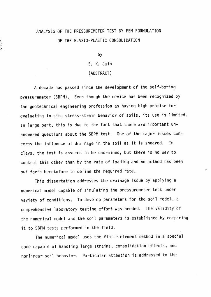
A decade has passed since the development of the self-boring

pressuremeter (SBPM). Even though the device has been recognized by

the geotechnical engineering profession as having high promise for

v evaluating in-situ stress—strain behavior of soils, its use is limited.

In large part, this is due to the fact that there are important un-

answered questions about the SBPM test. One of the major issues con-

cerns the influence of drainage in the soil as it is sheared. In

clays, the test is assumed to be undrained, but there is no way to

control this other than by the rate of loading and no method has been

put forth heretofore to define the required rate. °

This dissertation addresses the drainage issue by applying a

numerical model capable of simulating the pressuremeter test under

variety of conditions. To develop parameters for the soil model, a

comprehensive laboratory testing effort was needed. The validity of

the numerical model and the soil parameters is established by comparing

it to SBPM tests performed in the field.

The numerical model uses the finite element method in a special

code capable of handling large strains, consolidation effects, and

nonlinear soil behavior. Particular attention is addressed to the

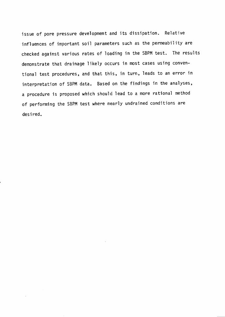
issue of pore pressure development and its dissipation. Relative

influences of important soil parameters such as the permeability are

checked against various rates of loading in the SBPM test. The results

demonstrate that drainage likely occurs in most cases using conven-

tional test procedures, and that this, in turn, leads to an error in

interpretation of SBPM data. Based on the findings in the analyses,

a procedure is proposed which should lead to a more rational method

of performing the SBPM test where nearly undrained conditions are

desired.

ACKNONLEDGEMENTS l

To Professor G. N. Clough, for his continuous encouragement and

guidance. without his assistance this dissertation would not have been

in existence.

To Professor J. M. Duncan, for his useful comments on the draft

of the dissertation.

To fellow graduate students in geotechnical engineering, for

their constant support and friendship.

To the National Science Foundation, for the financial support of

this investigation.

And, to the United States of America, the beautiful and wonderful

blessed land, for having me over here.

iv

TABLE OF CONTENTS

Page

ABSTRACT ........................... ii

ACKNONLEDGEMENTS ....................... iv

CHAPTER

1. INTRODUCTION ..................... 1

2. PRESSUREMETER THEORIES ................ 8

2.1 Menard Pressuremeter Test .........·. . . 81. The Un1oading Phase ............ 102. The Re1oading Phase ............ 103. The E1astic Phase ............. 104. The P1astic Phase ............. 14

2.2 Se1f-Boring Pressuremeter Test .......... 182.3 Stress-Strain Curve from Pressuremeter Data . . . 20

(a) Pa1mer-Bague1in—Ladanyi Method ....... 20(b) Oenby-C1ough Method ............ 23

2.4 Determination of Cvh from the PressuremeterHo1ding Test ................... 30

3. ELASTO-PLASTIC CONSOLIDATION: FORMULATION OF THEFINITE ELEMENT EOUATIONS ............... 33

3.1 Biot's Theory .................. 343.2 E1asto-P1astic Conso1idation ........... 373.3 PEPCO - The Finite E1ement Program ........ 39

4. LABORATORY TESTING OF SAN FRANCISCO BAY MUD ...... AQ

4.1 Samp1ing and Preserving Undisturbed Soi1 ..... 424.2 Unconfined Compression Tests ......... . . . 444.3 Oedometer Tests ................. 52

Samp1e Preparation ............... 57Stress Contro11ed Tests ............ 57Strain Contro11ed Tests ............ 58

4.4 Triaxia1 Tests .................. 61UU Test .................... 65Conso1idated Drained Tests ........... 65Conso1idated Undrained Tests .......... 69The Unconventiona1 Test ............ 76

r V

Page

5. MODELING OF SOIL BEHAVIOR: EVALUATION ANDVERIFICATION OF SOIL CONSTANTS ............ 815.1 Mechanism of Hardening in Meta1s ......... 815.2 Mechanism of Undrained Hardening in C1ays .... 845.3 Cambridge Soi1 Mode1s .............. 87

Mode1 Parameters ................ 93Undrained Strength in Cam C1ay ......... 96

5.4 Verification of Constitutive Mode1 ........ 98(a) Undrained Tests .............. 99(b) Drained Tests ............... 102

5.5 Conc1uding Remarks ................ 102

6. MODELING OF FIELD PRESSUREMETER TESTS: AXISYMMETRICPLANE-STRAIN ANALYSIS ................. 107

6.1 Mode1 Parameters ................. 1076.2 Comparisons: Fie1d vs. Mode1 .......... 1106.3 Simu1ation of Ho1ding Test ............ 125

7. EFFECT OF FINITE PRESSUREMETER LENGTH: THEAXISYMMETRIC ANALYSIS ................. 127

7.1 Simu1ation of Fie1d Tests ............ 1287.2 Observations in the Vertica1 P1ane ........ 1357.3 Cost Ana1ysis: Axisymmetric vs. P1ane—Strain . . 141

8. DRAINAGE DURING SHEAR IN THE PRESSUREMETER TEST .... 144

8.1 Effect of Permeabi1ity in Mode1ing Actua1 Test . . 1448.2 Genera1 Effect of Variation in Permeabi1ity . . . 1458.3 Effect of Rate of Loading ............ 1528.4 Effect of Permeabi1ity and Loading Rate ..... 1618.5 Recommended Procedure for Conducting 4

Pressuremeter Tests ............... 164

9. SUMMARY AND CONCLUSIONS ................ 165

9.1 summary ..................... 1659.2 Conc1usions ................... 166

REFERENCES .......................... 169

APPENDIX1. STRESS-STRAIN RELATIONS ................ 176

A1.1 Undrained Deformations ............. 179

( vi

Page

2. LABORATORY TEST DATA FOR SAN FRANCISCO BAY MUD .... 180

3. A NOTE ON MULTI-SURFACE HARDENING MODELS ....... 199Para11e1 Mode1 ................... 200Series Mode1 .................... 203Integrated Hardening Mode1 ............. 203Discussion ..................... 205

4. CUBICAL TESTS DESIGNED TO SIMULATE PRESSUREMETER‘ LOADING . .'...................... 208

VITA ............................. 214

vii

CHAPTER l

INTRODUCTION

Almost thirty years have passed since the first practical version

of the pressuremeter was introduced by Menard (l956). The basic idea

involved drilling a hole in the ground, inserting a cylindrical probe

into the hole, and expanding a membrane which surrounded the probe into

the sides of the hole. Fundamentally, the pressuremeter represents a

cavity expansion experiment, and soil parameters are obtained from the

pressure — volume curve derived from the test. The basic Menard type

of pressuremeter test has attained a considerable degree of popularity

but remains hampered by the stress relief and disturbance in the pre-

drilling process. Improvements and modifications to the original

approach have been made, with one of the most notable involving the

addition of a self - boring capacity. Developed almost simultaneously

in France and England, the self - boring probe is designed to drill

itself into the ground allowing the body of the instrument to maintain

intimate contact with the ground. This process then avoids the stress —

relaxation effect associated with opening the hole for the Menard

probe and supposedly minimizes disturbance. The test with a self -

boring pressuremeter (SBPM) involves the same principle as the basic

Menard procedure, although the methods of measuring response have been

upgraded and capabilities to monitor pore pressure development have

been added (wroth and Hughes, l974).

l

2

The inherent virtues of the SBPM test have been cited in a

number of publications. According to an MIT report to the Federal

Highway Administration (Ladd et al., l980), "The self—boring test

offers the theoretical potential of making measurements of in-situ

lateral stress and undrained stress-strain properties of saturated

clays in greater detail and more accurately than heretofore possible.

This is an exciting prospect which has received well deserved acclaim."

A similar view was expressed during a l983 National Science Foundation

workshop on experimental soil engineering held at Virginia Tech. As

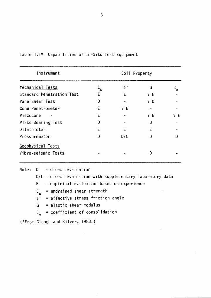
seen in Table l.l, excepting for the pressuremeter, in-situ test can

yield only a very limited infonnation regarding soil properties and

by-and—large their interpretation remains empirical. Moreover, only

the pressuremeter can be used to assess the strain softening properties

of the soil because, "the test has the special virtue that it is always

stable, in the sense that the pressure necessary to produce monotonic

expansion of the membrane always increases even though the soil may be

responding in a strain-softening manner; this is due to the fact that

the size of the element of soil undergoing the test is 'infinitely'

large" (Clough and Silver, l983).

In spite of the inherent virtues of this test, it has yet to be

truly accepted in geotechnical engineering. Presently, the evidence

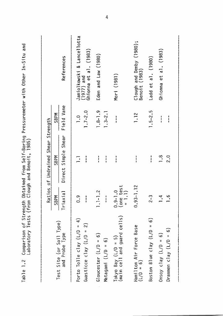
from field investigations is mixed. As shown in Table l.2, the un-

drained shear strength which is derived from the SBPM is often con-

siderably higher than that from other conventional tests. Many reasons

for this discrepancy have been put forth, including length to diameter

ratio of the probe, disturbance, rheological characteristics of the

3

Tab1e 1.1* Capabi1ities of In-Situ Test Equipment

Instrument Soi1 Property

Mechanica1 Tests Cu ¢' G CVStandard Penetration Test E E ? E —Vane Shear Test D - ? D -Cone Penetrometer E ? E — -Piezocone · E - ? E ? EP1ate Bearing Test D — D -Di1atometer E E E -Pressuremeter D D/L D D

Geophysica1 TestsVibro-seismic Tests — — D -

Note: D = direct eva1uationD/L = direct eva1uation with supp1ementary Iaboratory dataE = empirica1 eva1uation based on experienceCU = undrained shear strength ·¢' = effective stress friction ang1eG = e1astic shear modu1usCV = coefficient of conso1idation

(*From C1ough.and Si1ver, 1983.)

G4-)-I-) •n

'Q Q fiC 1- G(5 1- rs G z-

GJ (*7 CN (*73 U OO -*~ fi G

4-) (D C CN O LI rx Qä*1- GJ fü 1*- G G 1-U) U .1 -« CN >; OO

-I C 1- .¤ CNC GJ G5 • sz C 1*- •!-I L IG Q)!-x Ca 1-

GJ ··- fu 3 cm fcL W- X fü rx G •CI) GJ I/)°G4-) CI 1- GCN 1- 4-)C G ECG) G CFC fü GJ-4-) Ofü 'C CN G--G X G C IG 4-) G

1--C fü-

.C-I-* GJ CC OI\C O7*1- C+9 '1"I\O C *1- DO 'C C·1·· ECN·1- GJ L CC 'C *1-3 G1-—C 'O O 1—GJ fü CS- "J--G 1.1.1 E um ‘..1 c:)GJ4-) GJGJ CE r¤ 0 cw •- •.oGJ j • • • Q] •

L O. G GI 1- CU I 1- KI I I3 C G 'O • I I I I • I I IU) 4-) (/7 1-- FC I\ G G I IG LO I IU', Q) • • • •GJ C °Y* IG 1- IG

1-·L GJ LI.Q. L4-)C7 (/7 Lcz- fü'GLO L CULG fü COCN GJ (/7Gr- C

I (/7 GJQ- ^ IG1-+-) °U G- 1*- I I I I I I Gq)••—- GJ C E • I I I 1 I I • •(./)O C G *1- FC I I I I I I 1- C\I

C ·1·· (/7 (/7EGJ GOG L 4-*

-L 'C U‘+—‘C C GJC G L

"CG *1-GJ II- GCC O-1-C7 4-) CUG3 I./7 I/7 IG-1->O O 1- (U GGJ- •_Qp-· ••-· fü • •-I—)1- 1-GC.) 4-) E ·1·· CN I 1- I 1-· • I (*7 <' RD

G D. X • I I I IGJ1- (*7 I • •CE 1 G fü G I 1- I CNC CN C\.I 1- 1--I—)O (/> *1- • •CII •GL L 1- QL; QC‘·I·- I-QjxzL

U) 1-U) r- <I' 1- LD

I-I—GJ GJ r- 1-01- ¤. II N cu GJ II

>5 U U') r-C>; I- G II fü G COOL GJ \ «- 'U cm \ f-mo •—¤. .1 Q kO AL .1 LO II

*1--|-J •r->, Ca es Lßfü Q) ~./Lfü O}- ...1 II CO 3 U II GGL (/7 >~1-“ II C7 L >, \Q.O GJ fü G II O G G —JEL L.C} 1- >; \ G'C L1. 1- \~/OG OO U G .I G \C U ..IG.1 ~—-L ¤—

-\ .|fü L -' >a

C GJ U .I -« ·1·· GJ fü<\! —I—)'C 1- GJ GJ >»1- «·- 1- fü U• *1-C O U -I-) *1- GGJ CCC G 1-1— (/)G I·— U U) E GU O U C

*1- GJ fü -I-)II C GJGJ -I-) O -I-) U O7 OC 1- O >5 E1- (/7 4-) (./7 3 G >;•r- •1-G +-) O E.Q GJ L fü O -1-> XG E\ U) U7 füG I- O 3 r- G OE fü...I O C L1- C G G Z I--- I~/ G G G

5

soils, and dissipation of pore pressures in the soil around the probe.

Recently, a number of research studies have begun to focus on the

issues surrounding the SBPM test. Often these consist of theoretical

or field investigations, yet rarely are the two efforts combined.

One of the most persistent questions concerning all forms of

pressuremeter test is the effect of, or existence of, dissipation of

excess pore pressures set up in the soil during the test. This is im-

portant in clays and silts since the test results are analyzed assuming

that the test is undrained. Inasmuch as the only control on the

drainage is through the rate of loading, the most often asked question

in the pressuremeter literature is how rapidly the test should be con-

ducted. "Is partial drainage an important consideration?" asks the

MIT report. "If so, what expansion rates are required to achieve

acceptable results?" The "...theory has not provided guidelines regard-

ing suitable rates as a function of the consolidation characteristics

of various soil types." This is one of the objectives of this dis-

sertation, to guide the engineer concerning the rate at which the test

is to be conducted so it is virtually undrained, and what to expect

should the test be conducted below the prescribed loading rate.

The rate of loading can have substantial influence on the results

of the SBPM test. Under very slow loading rates, the soil can

experience drainage. Since there is no way for the engineer to know

if the drainage occurred, he analyzes the results assuming that no

drainage took place. As shown in this dissertation, this leads to an

underestimate of the shear strength. On the other hand,’very fast

loading rates will overpredict the shear strength of soil due to

6

rheological effects. Since the rheological or time effects are not

accounted for in the interpretation of the pressuremeter test data, an .

optimum loading rate has to be found for each soil at which the

drainage just begins to take place.6

Recently, in a Ph.D. investigation by Benoit (l983) under the

supervision of Dr. G. W. Clough, a series of SBPM field tests were per-

formed in a deposit of soft clay to examine the influence of rate of

loading and disturbance on test results. These tests utilized state-

of-the-art technology in the equipment and provided a solid data base.S

while the information derived was useful, it left questions unanswered

because the pressuremeter measurements can only be made at the face of

the cavity. Response in the soil medium away from the cavity is not

known.

This thesis is directed towards providing the theoretical basis

for the phenomena observed in the Benoit tests. In the process an

analytical tool is developed and verified which can be used to assess

the question of relative effects of pore pressure dissipation and dis-

turbance on pressuremeter test results. The methodology is thereafter

used to provide a means of predicting the rate at which a pressuremeter

test should be performed to achieve suitably undrained conditions to

yield realistic soil parameters.The finite element method is used in this work as it is the only

available technique for analyzing problems where the material is to

be modeled as a porous elasto-plastic medium with a capability of

coupled consolidation. A finite element mesh permits the examination

of the states of stress and strain, and the developed pore pressures

7

in the entire soil medium during all stages of the pressuremeter

test.

Following this introduction, Chapter 2 briefly describes the

Menard and the self-boring pressuremeter tests, and presents a review

of the pressuremeter theories which are needed for deriving the

engineering properties of soils from the pressuremeter test data. The

finite element soil model is described in Chapter 3. Chapter 4 sum-

marizes the laboratory testing of the San Francisco Bay Mud, undertaken

in order to determine the soil constants for the model. Subsequently,

validity of the soil model is examined, against the laboratory tests

in Chapter 5, and against the field pressuremeter tests in Chapter 6.

Soil model is then used in Chapter 7 for a detailed analysis of the

SBPM test. Finally, the Chapterääaddresses the important question of

drainage in the SBPM test.

CHAPTER 2

PRESSUREMETER THEORIES

The problem of expansion of a cylindrical cavity in a semi-

infinite medium has been a subject of study for decades. The

analysis proceeds as a limiting case of the problem of thick walled

tube whereby an expansion curve relating radial strain and the internal

pressure is derived once the material properties of the medium are

specified. In the pressuremeter test, we attempt to solve an inverse

problem. Given the expansion curve of a cylindrical cavity-—derive the

material properties.

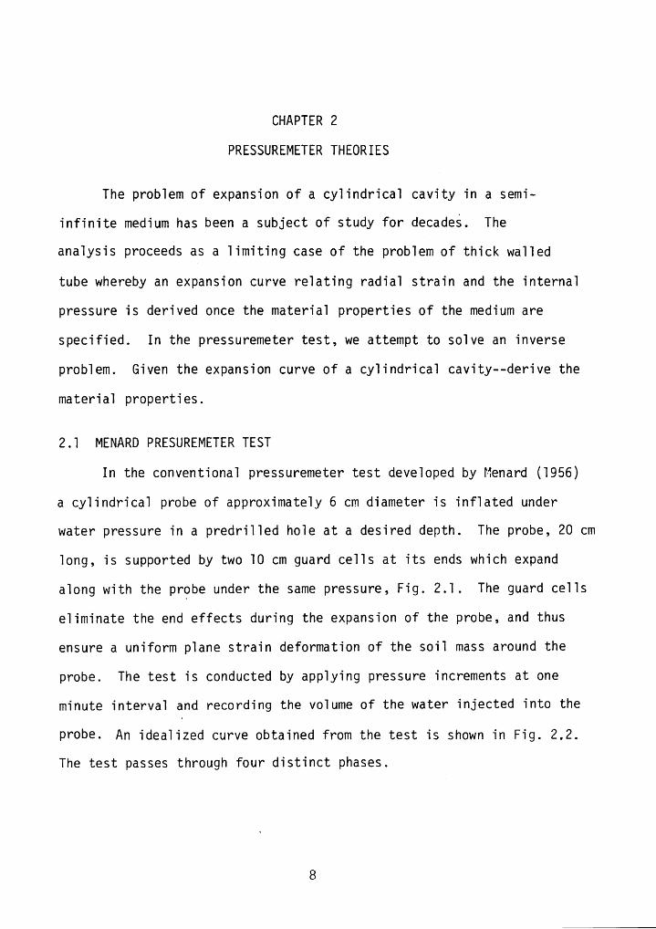
2.l MENARD PRESUREMETER TEST

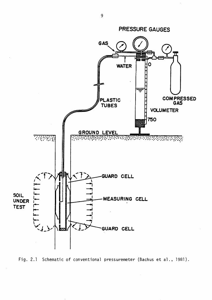
In the conventional pressuremeter test developed by Menard (l956)

a cylindrical probe of approximately 6 cm diameter is inflated under

water pressure in a predrilled hole at a desired depth. The probe, 20 cm

long, is supported by two l0 cm guard cells at its ends which expand

along with the probe under the same pressure, Fig. 2.l. The guard cells

eliminate the end effects during the expansion of the probe, and thus

ensure a uniform plane strain deformation of the soil mass around the

probe. The test is conducted by applying pressure increments at one

minute interval and recording the volume of the water injected into the

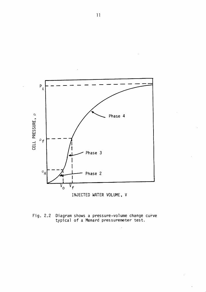
probe. An idealized curve obtained from the test is shown in Fig. 2.2.

The test passes through four distinct phases.

8

9

PRESSURE 6110666G6 ®\ -_ Ö“’wasn {

II

[ „ I' I[ I1TUBES |/2 : VOLUMETER

750. . ,.. ... .....,.

2* (V 6uAn0 661.1.1 _ Q \S: §L- E Q MEASURING 661.1.. E —•1 'TEST [ __, _1.. g E {-1

GUARD661.1.Fig.

2.1 Schematic of 60nventi0na1 pressuremeter (Bachus et a1., 1981).

10

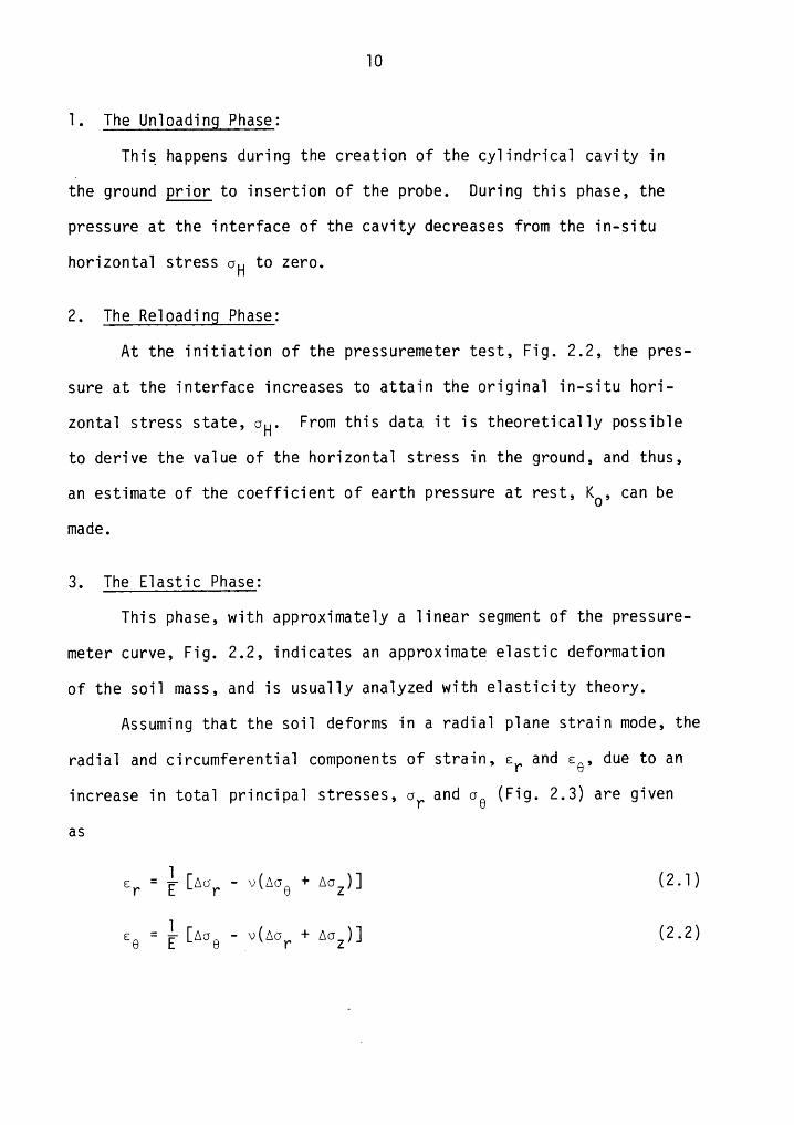
1. The Un1oading Phase:This happens during the creation of the cy1indrica1 cavity in

the ground prigr_to insertion of the probe. During this phase, the

pressure at the interface of the cavity decreases from the in-situ

horizonta1 stress 6H to zero.

2. The Re1oading Phase:At the initiation of the pressuremeter test, Fig. 2.2, the pres-

sure at the interface increases to attain the origina1 in-situ hori-

zonta1 stress state, 6H. From this data it is theoretica11y possib1e

to derive the va1ue of the horizonta1 stress in the ground, and thus,

an estimate of the coefficient of earth pressure at rest, K6, can bemade.

3. The E1astic Phase:

This phase, with approximate1y a 1inear segment of the pressure-

meter curve, Fig. 2.2, indicates an approximate e1astic deformation

of the soi1 mass, and is usua11y ana1yzed with e1asticity theory.

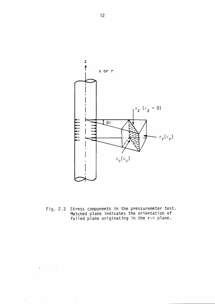
Assuming that the soi1 deforms in a radia1 p1ane strain mode, the

radia1 and circumferentia1 components of strain, 6P and 66, due to anincrease in tota1 principa1 stresses, 6r and 66 (Fig. 2.3) are given

as

(2.1)

66 = é [M16 — 'v(AoY_ + M1Z)] (2.2)

II

. PQ}

C: \ Phase 4E

LUx: .

Ecxc;.1 pf I3 IJg Phase 3 ÄI

IOH A',-I-· Phase 2I

Vo VfINJECTED WATER VOLUME, V

Fig. 2.2 Diagram shows a pressure-voIume change cuhvet_y|D'IC&I of 6 M€I'IöY‘CI pY‘€SSUY‘€ITI€'IZ€Y‘ test.

l2

-T x or r4Ih*

OZ (EZ = O)

o@(c6)

1IP*

Fig. 2.3 Stress components in the pressuremeter test.Matched plane indicates the orientation offailed plane originating in the r—n plane.

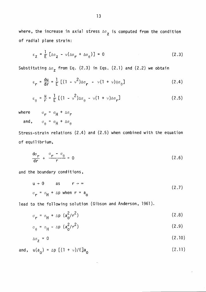
l3

where, the increase in axial stress Adz is computed from the conditionof radial plane strain:

ez [A0Z — v(A0r + A0o)] = Ü · (2.3)

Substituting Adz from Eq. (2.3) in Eqs. (2.l) and (2.2) we obtain

Er - gg = g ((1 (2.4)

eo = $—= g [(l — v2)A0o - v() + v)AGr] ( (2-5)

where dr = dH + Adrand, 0o = 0H + Aoo

Stress-strain relations (2.4) and (2.5) when combined with the equation

of equilibrium,

d0 G — Gr Y' G =-aF— + r 0 (2.6)

and the boundary conditions,

u —> 0 as r —> <>¤(2.7)

0r=0H+Apwh€nY‘=aO

lead to the following solution (Gibson and Anderson, l96l).

dr = dH + AD (ag/r2) (2 8)0o = 0H — Ap (ag/r2) (2.9)

Adz = 0 (2-l0)and- Mao) = AP [(l + v)/Elao (2-ll)

14

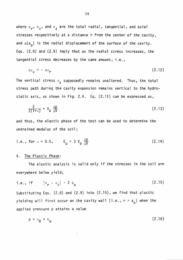
where 6r, 66, and 62 are the tota1 radia1, tangentia1, and axia1

stresses respective1y at a distance r from the center of the cavity,

and u(aO) is the radia1 disp1acement of the surface of the cavity.

Eqs. (2.8) and (2.9) imp1y that as the radia1 stress increases, the

tangentia1 stress decreases by the same amount, i.e.,

A66 = - A6r (2.12)

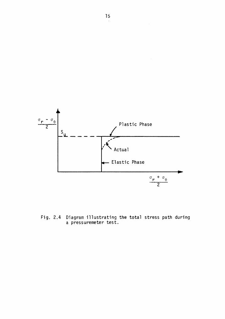
The vertica1 stress 62 supposed1y remains una1tered. Thus, the tota1stress path during the cavity expansion remains vertica1 to the hydro-

static axis, as shown in Fig. 2.4. Eq. (2.11) can be expressed as,

E - AE‘("T21+6 ‘ V6 AV (2*13)and thus, the e1astic phase of the test can be used to determine the

undrained modu1us of the soi1;

· Z = ABi.e., for v 0.5, EU 3 VO AV (2.14)

4. The P1astic Phase:

The e1astic ana1ysis is va1id on1y if the stresses in the soi1 are

everywhere be1ow yie1d;

i.e., if |6r — 69l < 2 cu (2.15)

Substituting Eqs. (2.8) and (2.9) into (2.15), we find that p1astic

yie1ding wi11 first occur on the cavity wa11 (i.e., r = ao) when the

app1ied pressure p attains a va1ue

p = GH + gu (2.16)8

l5

6 - 6—I¥?——Q- Plastic Phase_•-_ _- I

I ActualElastic Phase

or + 692

Fig. 2.4 Diagram illustrating the total stress path duringa pressuremeter test.

T6

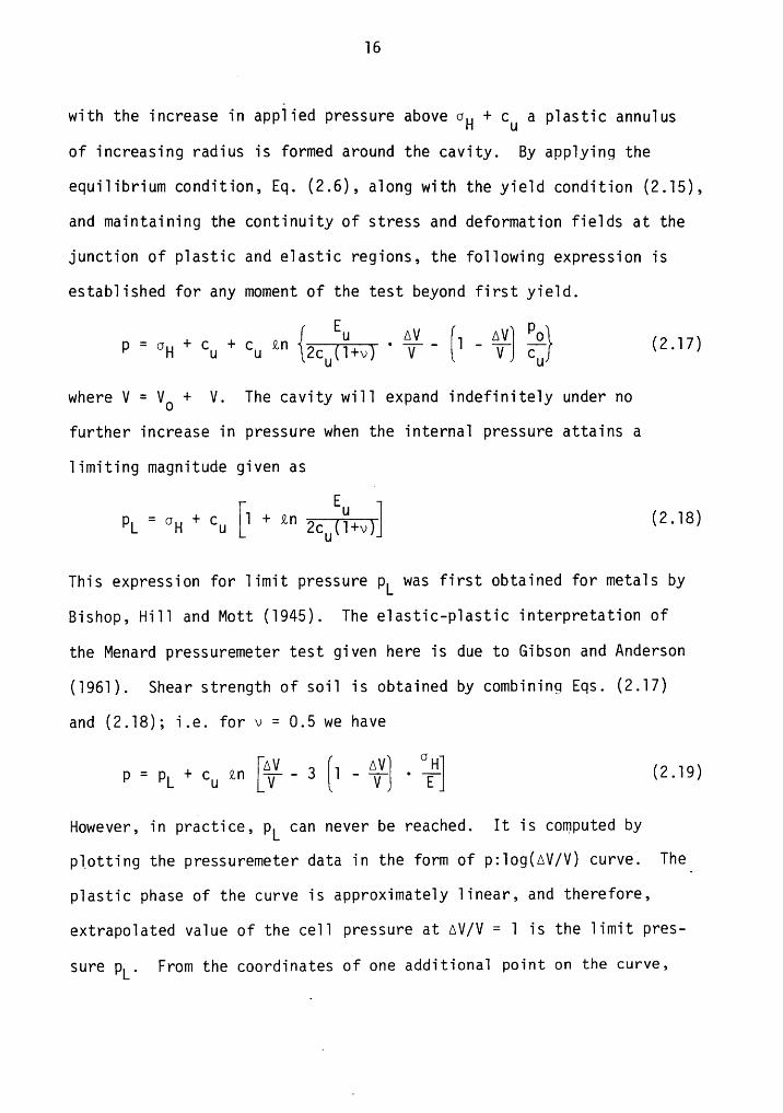
with the increase in applied pressure above 6H + cu a plastic annulus

of increasing radius is formed around the cavity. By applying the

equilibrium condition, Eq. (2.6), along with the yield condition (2.l5),

and maintaining the continuity of stress and deformation fields at the

junction of plastic and elastic regions, the following expression is

established for any moment of the test beyond first yield.

p = 6H + cu + cu ZH

[TwhereV = VO + V. The cavity will expand indefinitely under no

further increase in pressure when the internal pressure attains a

limiting magnitude given as

p = 6 + c [T + Zn EU (2 T8)L H u ÖEETTYÜT °

This expression for limit pressure pL was first obtained for metals by

Bishop, Hill and Mott (T945). The elastic-plastic interpretation of

the Menard pressuremeter test given here is due to Gibson and Anderson

(l96l). Shear strength of soil is obtained by combining Eqs. (2.l7)

and (2.T8); i.e. for v = 0.5 we have

p = pL + cu tn 3

{THowever,in practice, pL can never be reached. It is computed by

plotting the pressuremeter data in the form of p:log(AV/V) curve. The.

plastic phase of the curve is approximately linear, and therefore,

extrapolated value of the cell pressure at AV/V = T is the limit pres-

sure pL. From the coordinates of one additional point on the curve,

l7

the shear strength cu can be computed from Eq. (2.l9).

The determination of E and cu completely defines the stress-

strain curve for the elastic-perfectly plastic material. However,

for soft clays the parameters obtained by the Menard pressuremeter

have been found far from in agreement with other conventional field

and laboratory tests though reasonable modulus values are obtained for

stiff clays.

As mentioned by Ladd et al. (l980) intensive efforts were made by

Menard and co-workers in France to correlate their pressuremeter

values of modulus and strength to those obtained from "conventional"

tests. Results were discouraging. Hence, they decided that the

pressuremeter test be viewed as a "model foundation test," which could

become a basis for designing shallow and deep foundations with the use

of empirical scaling factors. The book by Baguelin et al. (l978)

presents a comprehensive treatment to foundation design by the

pressuremeter.

Ladd et al. (l980) indicate that a practice of employing the

Menard Pressuremeter Test for in-situ measurement of soil properties

for use with conventional theories to predict stability, deformations,

in-situ stresses, etc., is "ill-advised." The reasons include: a

substantial disturbance of soil during the unloading and reloading

phases, the unknown drainage conditions, and the simplifications made

in the methods of interpretation by assuming soil an elastic-perfectly

plastic material.

l8

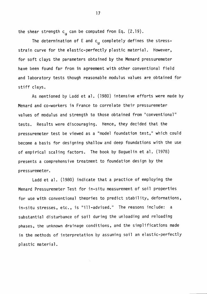
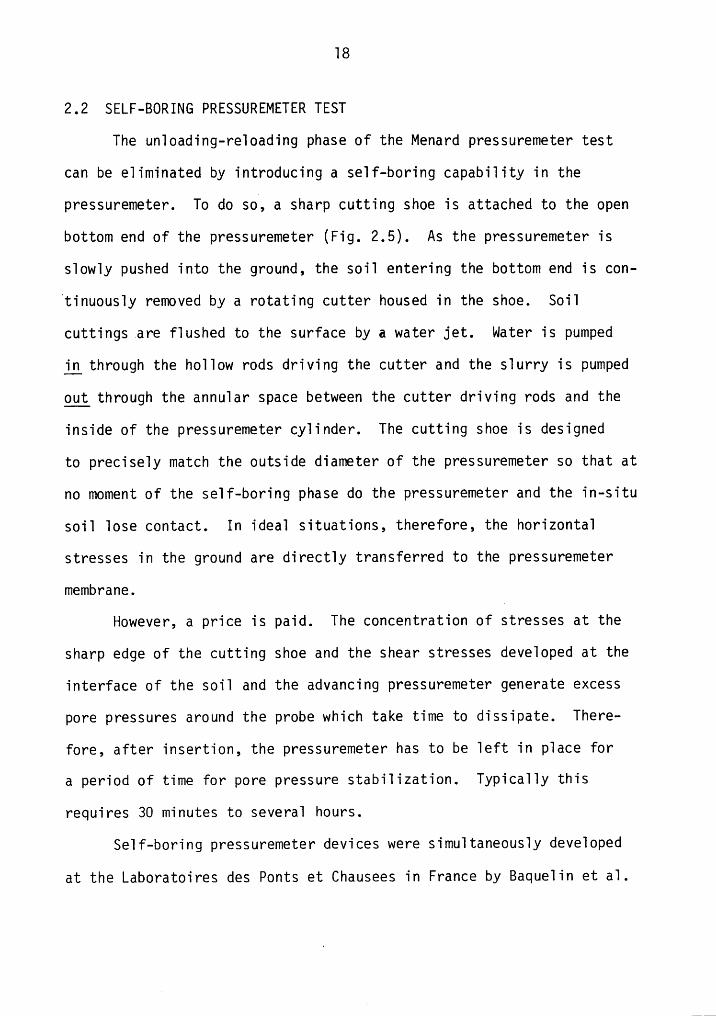
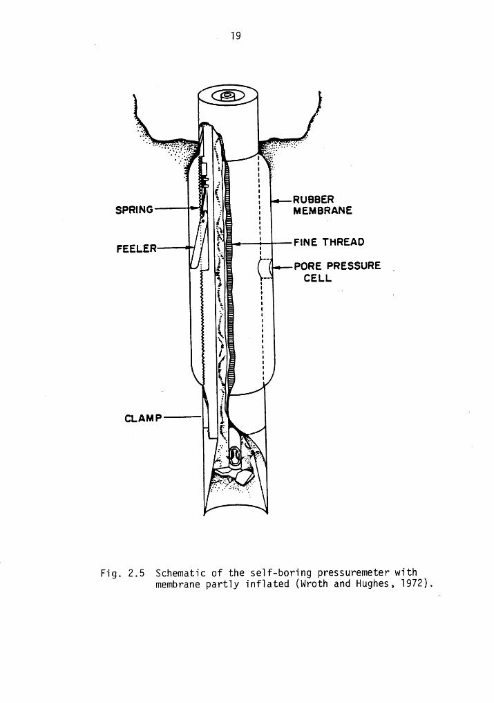
2.2 SELF-BORING PRESSUREMETER TEST

The unloading-reloading phase of the Menard pressuremeter test

can be eliminated by introducing a self-boring capability in the

pressuremeter. To do so, a sharp cutting shoe is attached to the open

bottom end of the pressuremeter (Fig. 2,5). As the pressuremeter is

slowly pushed into the ground, the soil entering the bottom end is con-

‘tinuously removed by a rotating cutter housed in the shoe. Soil

cuttings.are flushed to the surface by a water jet. water is pumped

jg_through the hollow rods driving the cutter and the slurry is pumped

gut through the annular space between the cutter driving rods and the

inside of the pressuremeter cylinder. The cutting shoe is designed

to precisely match the outside diameter of the pressuremeter so that at

no moment of the self-boring phase do the pressuremeter and the in-situ

soil lose contact. In ideal situations, therefore, the horizontal

stresses in the ground are directly transferred to the pressuremeter

membrane.

However, a price is paid. The concentration of stresses at the

sharp edge of the cutting shoe and the shear stresses developed at the

interface of the soil and the advancing pressuremeter generate excess

pore pressures around the probe which take time to dissipate. There-

fore, after insertion, the pressuremeter has to be left in place for

a period of time for pore pressure stabilization. Typically this

requires 30 minutes to several hours.

Self-boring pressuremeter devices were simultaneously developed

at the Laboratoires des Ponts et Chausees in France by Baquelin et al.

I . 19

i ä! * I} RussenSPRING „ msmannna‘ I ä .

FEELER Fans THREAD1 Q PORE Pnsssuns _‘ E é CELL

ÄI

c1.A~u¤-——- § 1Fgi ,

.2l}<*§>LI·

Fig. 2.5 Schematic of the se1f-boring pressuremeter withmembrane part1y inf1ated (wroth and Hughes, 1972).

20

(l972) and at the Cambridge University by wroth and Hughes (l972,l973).The French version is known as the Pressiometre Autoforeur while theEnglish version is called the Camkometer. The two versions differ inmechanical operations but the underlying principle is the same.

A schematic of the Camkometer is shown in Fig. 2.5. During thetest, the cavity is expanded by applying gas pressure from inside thepressuremeter cylinder. The radial displacement is measured by track-ing the movement of the membrane electronically by means of three

strain feeler arms located l2O degrees apart at mid-height in the

probe. The pore pressures are recorded by transducers which are placed

in the membrane wall to move with the expanding membrane. The detailsof a complete self-boring unit and the test procedures have been

given by Denby (l978) and Benoit (l983).

2.3 STRESS-STRAIN CURVE FROM SBPM DATA

(a) Palmer-Baguelin-Ladanyi Method:

In part, success of a pressuremeter test lies in the interpreta-

tion method used for determining the engineering properties of the soil.

As shown in the preceeding discussion, Gibson and Anderson (l96l)

employed the theory of elasticity to determine the shear modulus, and

the theory of plasticity to derive undrained shear—strength of soil from

the pressuremeter data. Subsequently, an impetus to the pressure-

meter test was given by Baquelin et al. (l972), Ladanyi (l972) and

Palmer (l972) who proposed an analytical technique to derive the

complete stress-strain curve from the pressuremeter data. The soil is

assumed to follow a stress-strain relationship of the form

2l

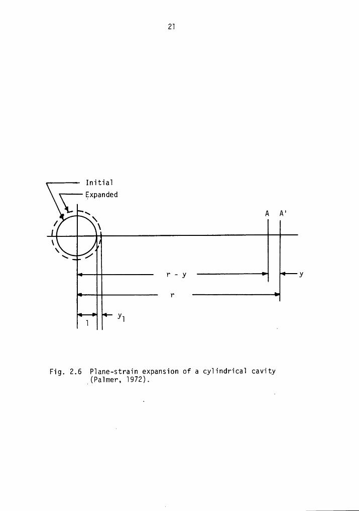
InitialTExpanded~ A A·[ x\

1\

“ ÄII yI ”

y1 1

Fig. 2.6 Plane-strain expansion of a cylindrical cavity_(Palmer, l972).

22

0;* - 01; = 1°(61__ — 69) (2.20)Making the second important assumption that the soil will shear underundrained conditions, then it follows that

66 = — 61„ (2.2l)

the Eq. (2.20) can be simplified to

01; - 01;) = l°(6G) 1 (2.22)

Combining Eq. (2.22) with the equation of equilibrium (2.6), we get

ä — - l f( ) (2 23)dr ” r E6 ‘

Consider a cavity of unit radius. Under an applied pressure 0r(aO), ifthe cavity radius increases by y1 and the material point A, Fig. 2.6,moves outward by y, then the condition of no change in volume demandsthat

urz - n(r-y)2 = ¤(l+y1)2 - ·¤(l)2 (2-24). 21.e., y = r - [rz — 5/1(2 + 5/1)]]/ (2-25)

1, 5/1 (2+5/1 )1 ]](2Therefore, 69 - Fjy-— - l + [l — ——;;y-——U (2-26)Since or changes from the applied pressure ¤P(a0) at ao = l + y1, to0H at infinity, Eq. (2.23) can be integrated to have

da = -( gf (66) ar (2.27)l+y1 l+y1

·„

1 y1(2+y1)--l/2(2 28)]|•€•, ' " F f ' 1 + ' •

23

The stress-strain relation is determined by solving Eq. (2.28) forthe unknown function f. As shown by Palmer (l972), the following rela-

tion is obtained,

do (61)= r 0fb/1) y](l + y])(2 + xl) d Y1 (2-29)That is, at the wall of the cavity

dcrar - ag = 6r(l + er)(2 + er) EE; (2,30)

For small strains, Eq. (2.30) reduces to a particularly attractive form

0 - 0 dor 0 = __r;———j?——— er d€ (2.3l)r

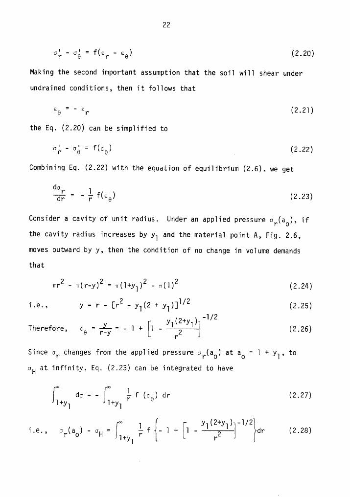
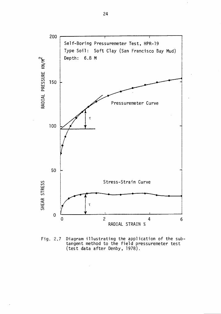
Eq. 2.3l, regarded a milestone in the development of the self-boringpressuremeter, was independently arrived at by Palmer (l972),Ladanyi (l972), and Baguelin et al. (l972), Eq. 2.3l states that theproduct of the slope of the pressuremeter curve and the correspondingradial strain is the shear stress induced in the soil at the cavity

wall. Therefore, the complete stress-strain curve can be derived

from the pressuremeter curve by a simple graphical procedure. The

procedure, known as the subtangent method, is illustrated in Fig. 2.7.

(b) Denby—Clough Method:

Eq. (2.3l) provides a link between the experimental pressure-

meter curve and a general stress-strain relation reflected in Eq.

(2.22). Given an explicit stress-strain relation, the equation for

24

200 1Self-Boring Pressuremeter Test, HPR—l9Type Soil: Soft Clay (San Francisco Bay Mud)

¤éE Depth: 6.8 M\Z¥1.1.1 _ ICEID3 160 IL1.1QS¤. ' I.1E [ I

PY‘€SSUY‘€ITl€'IZ€Y‘ CUTVE ICZ

_ T I

l00

50I-gg Stress—Strain CurveääI-aniä I

i I1Lu t IE I I

0 I0 2 4 6

RADIAL STRAIN %

Fig. 2.7 Diagram illustrating the application of the sub-tangent method to the field pressuremeter test(test data after Denby, l978).

25

the pressuremeter curve could be derived, or vice-versa. If the soil

is assumed to follow a particular type of stress—strain response, say

hyperbolic or Ramberg—0sgood type, the model parameters could directlybe derived from the pressuremeter curves.

Due to the erratic behavior of in-situ soils, often it becomes

necessary to assume the nature of stress-strain curve apriori. The

method of Palmer-Baquelin-Ladanyi requires that the slope of the

pressuremeter be determined at each point. Owing to the slight

disturbance caused during the insertion of the probe, it sometimes

becomes difficult to determine this slope in the beginning portion of

the curve. Considering that most clays require only l to 3% s-rain

to reach failure, and that the shear modulus is determined from the

initial slope of the pressuremeter curve it may be necessary to define

the beginning portion based on the prefailure stage of the curve. Such

an extension of the Palmer-Baquelin-Ladanyi theory was provided by

Denby and Clough (l980) through a hyperbolic formulation.

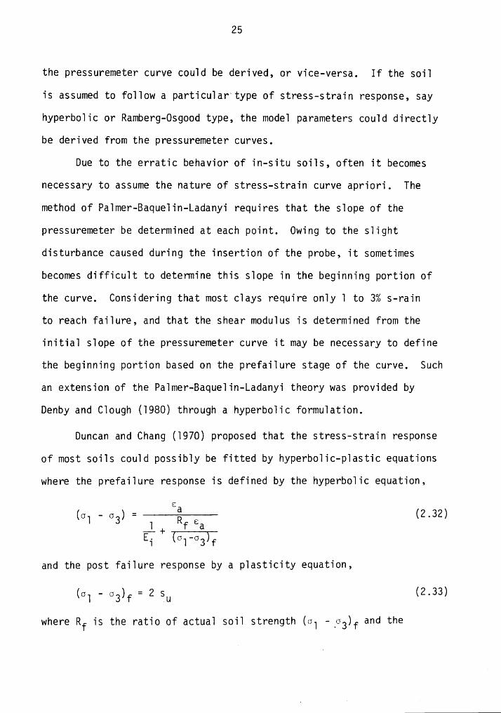
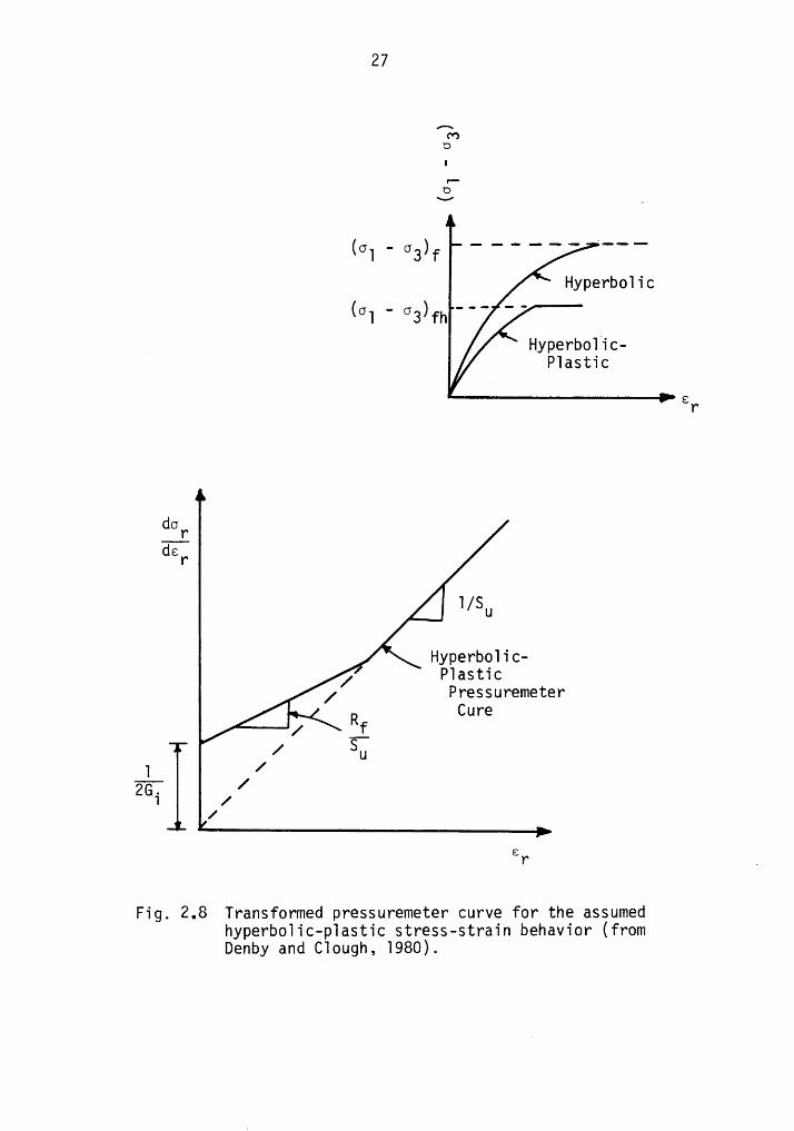
Duncan and Chang (l97D) proposed that the stress—strain response

of most soils could possibly be fitted by hyperbolic-plastic equations

where the prefailure response is defined by the hyperbolic equation,

— Ea 2 32)(Ü] ' Ö3) ‘ •Ei lääl?

and the post failure response by a plasticity equation,

(61 — ¤3)f = 2 SU (2-33)where Rf is the ratio of actual soil strength (61 — ¤3)f and the

26

asymptotic strength (6] - G3)fh, see Fig. 2.8. Rf has been found to

vary from 0.9 for soft plastic clays to 0.6 for overconsolidated clays

(Duncan et al. l980). Ei is the initial tangent modulus. For the

pressuremeter problem, this equation must be expressed in radial stress

and strain variables. Equating the engineering shear strain in the

pressuremeter to that of triaxial test, we get for the undrained condi-

tions

-ä2eY_—2ea Ai.e., (2.34)

EI :*%*6a 3 r

Noting that, Ei = 3 Gi, under undrained conditions, (6] - 63) in the

pressuremeter test is (6T - 66), and that (6V - 66)/2 is the undrained

shear strength su, Eq. (2.32) can be expressed as

O 'O El..‘%..2=..._%i.... (2.35)$+62i Su (

Relating this equation to Eq. (2.3l)

de ”Rr - .L LE6; ' 2Gi + su 6r (236)

Similarly, Eq. (2.23) can be combined with the Eq. (2.3l) to yield

de (2.37)r u

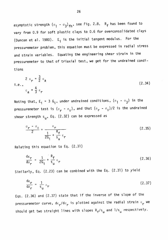
Eqs. (2.36) and (2.37) state that if the inverse of the slope of the

pressuremeter curve, dar/ÖOT is plotted against the radial strain Er we

should get two straight lines with slopes Ri/su and l/su respectively.

27

"?~»OI

if(°1 ‘ °2)1= '''""' I"-

Hyperbolic(°1 ' °3)fh '°° '°

R Hyperbolic—Plastic

Er

do..Lde r

l/SU

Hyperbolic-Plastic.//« Pressuremeter

R Cure/ .1i/ SU1 //

2Gi /zEr U

Fig. 2.8 Transformed pressuremeter curve for the assumedhyperbolic—plastic stress—strain behavior (fromDenby and Clough, l980).

28

Their junction defines the failure strain erf. As shown in Fig. 2.8,the first line has an intercept of l/(2 Gi) at er = 0. Therefore, su,

Rf, erf and Gi can readily be determined from one additional plot. Theinitial horizontal stress in the ground can be determined by integratingEq. (2.36) under the boundary conditions, or = oH for Er = O. Thefollowing expression is obtained.

Su RfoH = or - ä;-an [T + E; 2 Gi er] (2.38)

Interestingly enough, this equation represents the experimental

pressuremeter curve if the soil follows a hyperbolic stress—strain

relationship.

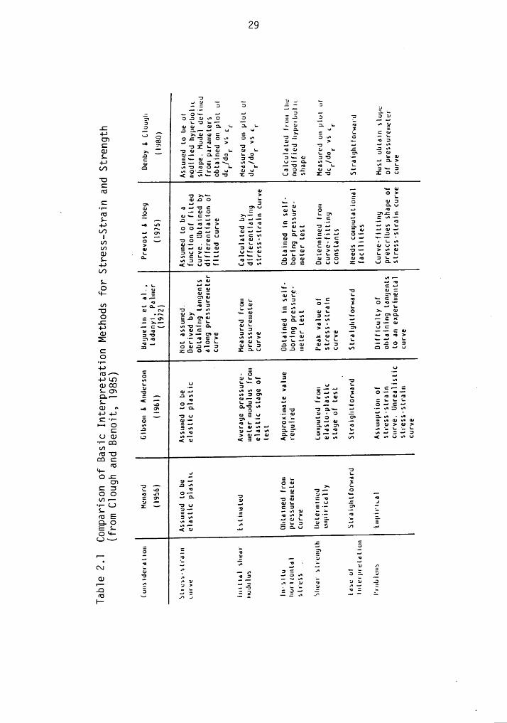
Dther interpretations of the pressuremeter test exist in the

literature. The pioneering work of Menard (l956) primarily rests on

empirical correlations. The interpretation given by Prevost and Hoeg

(l975) not only requires an elaborate computational effort but is

based on an assumption that the soil follows a "hyperbolic" response,

and not the "hyperbolic-plastic" as suggested by Duncan and Chang

(l970). The assumption of continuous hyperbolic response leads to high

shear strength for soils. A comparison of various available interpre-

tations is presented in Table 2.l.

Fortunately, during the course of present investigation the

author had to deal only with FEM pressuremeter curves which were so

well defined that the graphical subtangent method was more than

adequate.

-¤§

=

9

:

5

m

:__

__:.’3

.

'U

3

cc:

c

’*

-=>“"

0-·

5-*5

5

·

“=”¤£

-

P

3

-5***

:7

Q

Qägäa

_,

4;

3:0*-

3

_,,__

L.:

-

‘-/7

v•

'°·:7~^

1

31

(.303

>

J)

0

1,

Q

;

'..

3

ti

Ö

—·;

'=

°,;=-ä

,_

Ä:

._

(j)

mg

*•-L

3

22

0"‘""

g\

7:-

..,

L

V41.,

3:70

1:L.

5*)*

n

L

U

0

__,:

3

3

-

3-.:5

'·’

gz

ä

0

;;0

-:7*

5

c

3*=S

Z

5%

ä’1-

—

-C

°

v•°¤i“

>.=•

==;

5

*’

4-)

.;L.

<c>L..*!

3;:3

W

35:

L.

2-

°-

v‘Ü

O

,3;

Z

Z;

"’·;Z,'

3*3:

Ä-

:,,,0

2

_.°§

C

"

*‘

:

2::

5;.

7”:.•g\l

gg

Swan

"nw

P

-l‘•

c';

;

.;,3

4,,,

5g--

5;

3:v-

”",‘f„°

°'^

3***

•·¤

:*>"

5E*=

**3

1:***

5

°“°Ä°

-4->

:g°°

E

'Ü

U-!

<v“·-·

P

"°1

Lw

*¤cn"'

35‘*'

'—'!·E

5

°:

Q-

G

‘°m

·•-

Q)

'

cx

0,:0

25;,

„·-·

3

*!

L';

·-

•J·>cL

com

'Zf"

¤

__

Q1

5

o"-¤·

=

1:-*

EQ.,

..,

4;

vw

2;:m

§L.

SZ!

;,·-

:1

°0

EÄ

Ä

°·°ä··

:3

‘;i'5

Ä.

ät

„

‘

•-ß

"

31

r—

S5!

:23

Ug

j,

°3

3;,

~·ä

SE

'§·^.z

"cu

3

«·°

S'

"’;,·*

—-**2

L/im

::1,

U

.„

za-¤

Q

1;

L

>Q•

q_Q

0

U:

U

,¤

vwo

:1*".1•

r¤

°°c,·•°"

°13¤!

Q

·:1¤

'°

·-*

0

g

.:

3.,

·=

2;-EBZ

1:

°·

C

2-..

[*5

0*;

„·-•

*

"‘

O3

i·*

vb

2-

>·^

¥

LU

¤."'ä,

0g_E

1:

„—§g

3

zg§~

,_§§

Ä,.

3:*

‘°

u

6

Z

‘:

U3.

rz,

=·;,’··

2,*

A

~¤—¥¤

‘

__

U.)

>_‘..•

6

¤

.:1:

<„v•

2

Z50

1-

og

5::~°ä°‘3

äu

S3:

6-

S-,,,,

.

SGU

(J

gc.

"

L.:

~—"‘..1

Oo)

Q,

ää

.%§—

:-*,-5::

;

3

[__

:

H6

.

Z;

3

ß

L.

I

3

;

2E

gg:3

.3

g.

E

°

5

B20

·;·

*5:1

3,

···Z'°

:‘

.:·_

4

1*

S

E

E

"‘3

-2:35

2

;

Ä;

E3

.¤

gg;

..4

=•A

6

•

al

j

A

.n;_*^

A

0

v\·gg'

U

cg-

(5)*

U

•¤•

LV!

J?

1

62

-3

*-0u

A:

¤-5gll

:1,1*

11

6*,

:

E

é~=·ä

E-

t

Zt

W

kb

=,

6

3

„,,,

rg

I

U

,

_

:

..-_

„

6

U

BZ-

2

,,1*

..•-

-.2

iz];

'.;‘

E;

52

_

ä

,_g

i

Ü

¤

U"

L.-‘^

·—

2.

at^

Z-1

“-•

.

:7

A

5

3G./‘

,„"*

:2

2:

««

63

E..=

j

3O

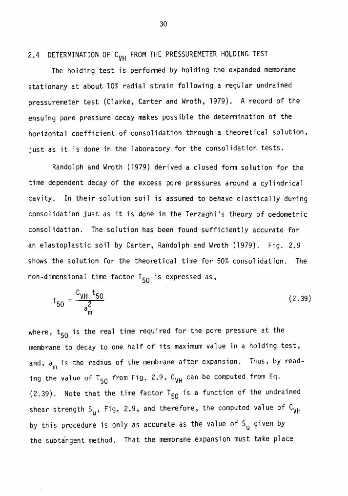
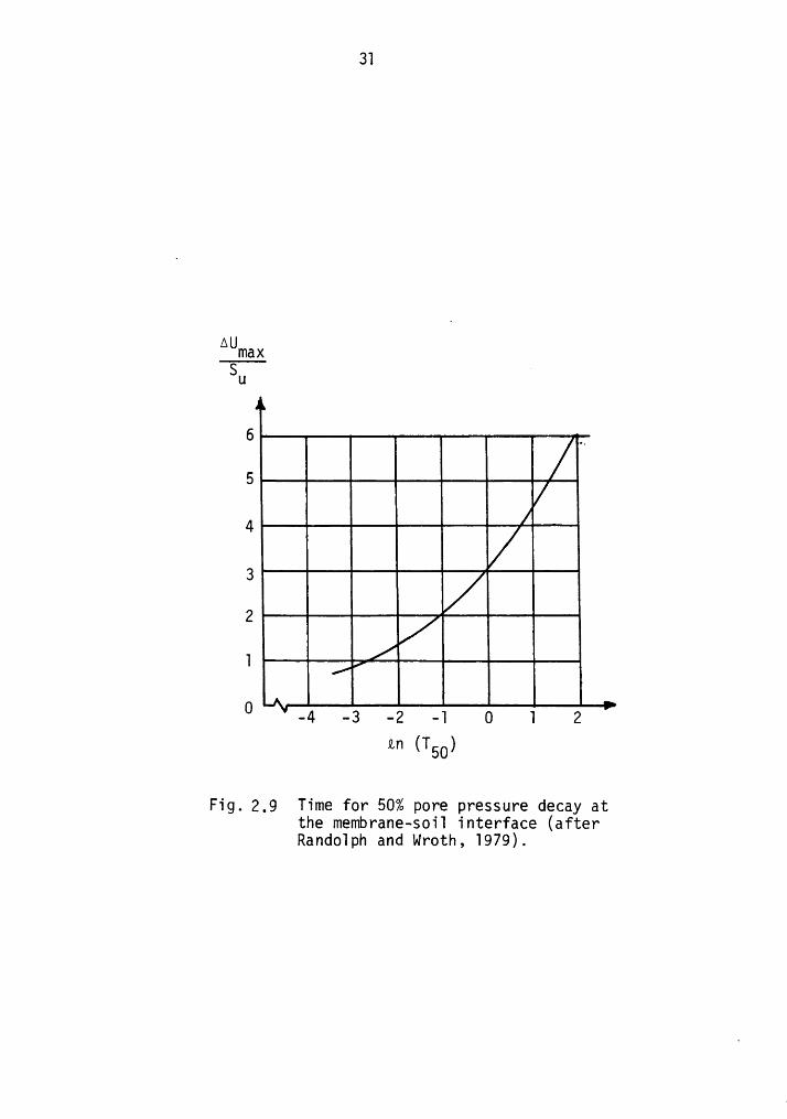
2.4 DETERMINATION OF CVH FROM THE PRESSUREMETER HOLDING TESTThe holding test is performed by holding the expanded membrane

stationary at about l0% radial strain following a regular undrained

pressuremeter test (Clarke, Carter and Wroth, l979). A record of the

ensuing pore pressure decay makes possible the determination of the

horizontal coefficient of consolidation through a theoretical solution,

just as it is done in the laboratory for the consolidation tests.

Randolph and wroth (l979) derived a closed form solution for the

time dependent decay of the excess pore pressures around a cylindrical

cavity. In their solution soil is assumed to behave elastically during

consolidation just as it is done in the Terzaghi's theory of oedometric

consolidation. The solution has been found sufficiently accurate for

an elastoplastic soil by Carter, Randolph and wroth (l979). Fig. 2.9

shows the solution for the theoretical time for 50% consolidation. The

non—dimensional time factor TSO is expressed as,

im = (2.:69)m

where, t50 is the real time required for the pore pressure at the

membrane to decay to one half of its maximum value in a holding test,

and, am is the radius of the membrane after expansion. Thus, by read-

ing the value of T5O from Fig. 2.9, CVH can be computed from Eq.

(2.39). Note that the time factor T50 is a function of the undrainedshear strength SU, Fig. 2.9, and therefore, the computed value of CVH

by this procedure is only as accurate as the value of SU given by

the subtangent method. That the membrane expansion must take place

3]

AU]T]äXSU ‘

6llIIIIH”5IlIIlIIAIIIIIÄI3IlII!IIZIIIIIIIIIIÜIIII0 -4 -2 -2 -1 0 1 2tn (T50)

Fig. 2.9 Time for 50% pore pressure decay atthe membrane—soi] interface (afterRand0]ph and wroth, ]979).

32

under undrained condition, acquires an unusual significance in the

success of a pressuremeter holding test.

In summary, this chapter reviews the pressuremeter theories which

are needed in order to derive the maximum possible information from a

SBPM test. It shows how the coefficient of earth pressure at rest,

KO, the undrained modulus, GV, the complete stress-strain curve, andthe coefficient of consolidation, CV, for the soil can be computedfrom the SBPM data. However, the information so derived is only as

accurate as the assumptions it is based upon. Therefore, emphasis here

is placed on the assumptions inherent in the pressuremeter theories.

The validity of the assumptions will be examined in the subsequent

chapters.

CHAPTER 3

ELASTO—PLASTIC CONSOLIDATION: FORMULATION

OF THE FINITE ELEMENT EQUATIONS

_ It is a common practice in geotechnical engineering to predict

the magnitude and the time rate of settlement from the Terzaghi

theory of consolidation. The magnitude is computed from the compres-

sibility of thesoil and the time rate from a heat conduction type

equation,

2cVä—§=§§§ (3.l)az

The underlying assumption of the Terzaghi theory is that the

vertical total stress increment, generated by the loading, remains

constant while the pore pressures dissipate. Thus, the theory does

not permit any redistribution of total stresses or pore pressures even· if the soil yields at some points during consolidation.

The three dimensional theory of consolidation formulated by Biot

(l94l) provided a coupling between the fluid flow and the deformation

of the soil skeleton. The total stress at any time in the medium is

determined through an interplay between the excess pore pressure and

the stress—strain relationship for the porous medium. Thus, it

is possible through Biot's theory to conduct an integrated analysis

of geotechnical problems in terms of stability and settlement. The

theory is particularly suited for the problem of partial consolidation

that we wish to address in this work.

33

34

3.1 BIOT'S THEORY

The following finite element formulation brings out the central

idea underlying Biot's theory of consolidation (Zienkiewicz, 1977). For

an elastic continuum, a standard discretized equation is expressed as,

[K] {6} = {R} (3.1)

in which [K] is the stiffness matrix and {R} constitutes the vector ofspecified forces. An analogous equation for the laminar fluid flow is

given as

{H1 {q} = {Rp} . . (3-2)where [H] is the fluid flow matrix, {q} the vector of pore pressures

at nodes and {Rp} is the applied flux.In conventional analyses, Eqs. (3.1) and (3.2) are solved

separately. Consequently, the compatibility of strains between the

elastic skeleton and the fluid is not ensured. Biot's theory satisfies

such a compatibility by coupling the motion of the fluid and skeleton

as follows.

It is known from the theory of seepage that in a saturated porous

elastic medium, the forces exerted by the pore fluid on the elastic

skeleton are given as,

_ X ax

2 ,, ÄBY py (3.3)

ällZ az

35

Zor,(xi} {Mi) (3.4)

Discretizing these forces in a finite element manner,

- -.ä_.{ Xi } {pxi } [Np] {Q} (3 5)

where, [Np] are shape functions relating the continuous values of the

pore pressures, p, to nodal values, {q}. Therefore, the nodal forces

contributed by the pore pressures are_ T _ T(F}p — fv [N] (Xi} dV —-[L] {Q} (3-5)

where, [N] are the displacement shape functions for the elastic

skeleton, and [L] the coupling matrix defined as,

T _ T 6(L} - (V (N} (Np} av (3.7)Consequently, for a porous elastic medium, Eq. (3.l) takes the

form

(K] (6} - [LJ] (4} = (R} (3.8)

Now, we wish to modify the Eq. (3.2) for the fluid-skeleton compati-

bility. The continuity equation is expressed as,

- • - ei M M MQ Bt [6x + 6y + 62) (3‘9)

where, the rate of discharge Q is equated to the rate of volume change

éii expressed in terms of the displacement components, u, v, and w of

the skeleton, Discretizing, Eq. (3.9)

6 6 T

36

The contribution of Q to Eq. (3.2) is,

IV [Np]T Q dV =-[L] gg {61 (3.ll)

Hence, for a porous elastic medium, Eq. (3.2) takes the form

[Hl iq) - [1.] ä 131 = (Rp) (3.12)

Suppose the solution (6V,qV) is known at time t1 and we are required to

find the solution (62,q2) at time t2 = tV + At. Employing the finite

difference technique, Eq. (3.l2) can be approximated in the form

[Hl 1qV+ 6<q2 — ql)1 A1; - [L] 132 - 311 = 0 (3.13)where 6 corresponds to the desired integration rule, e.g., B = 0.5

corresponds to the trapezoidal rule. Booker and Small (l975) have

shown that the above integration scheme is unconditionally stable for

B j_0.5. Eqs. (3.8) and (3.l3) can be assembled in a standard form as

V 1= (3.14)-L 6At H q2 —L6V - (l-B) At H qV

Thus, from the known solution at time tV, the solution can bedetermined at time t2.

The formulation of finite element equations incorporating

Biot's theory began with the work of Sandhu and wilson (l969) who

derived these equations by minimizing a Gurtin type energy functional.

A much simpler procedure utilizing the principle of virtual work was

later devised by Small, Booker, and Davis (l976). Following the

similar approach, Carter, Booker, and Small (l979) obtained the

discretized consolidation equations for a soil subject to finite

37

deformations. It is this formulation which is used in this investi-

gation through a finite element program named PEPCO, described sub-

sequently. The final set of equations are of the form shown above,

Eqs. (3.l4).

3.2 ELASTO-PLASTIC CDNSOLIDATION

The equations of Biot's consolidation theory can be used to

model elasto-plastic consolidation by replacing the elastic stress-

strain matrix [De] in the stiffness expression

[K] [Bl dV (3-lB)

by a suitable elasto-plastic constitutive matrix [DBB] for the soil

skeleton. A standard technique for deriving elasto-plastic matrix is

explained in Appendix l. In three dimensions, the matrix is expressed

as follows (Banerjee and Stipho, l978).

{ai = [pgp] {aie T e[DA

+ {al [D ] {al

where {6}] = [aF/aa aF/aa aF/aa . ], X, y, Z ' '

The parameter A is defined in Appendix l. In this work, the Modified

Cam Clay model is used which defines its yield curve as

2 2F=pM

where the mean effective stress p' and the octahedral shear stress q

are given as,

38

0); + o' + oé1>' = ————§—— (3.18)

.. I _ I 2 I I 2 I I 2q — ~/[2 [(¤X ¤y) + (¤y - ¤Z) + (¤Z - ¤X)2 2 2+ 6 Txy + 6 Iyz + 6 Izxil} (3.19)

M is the critical state parameter, defining the slope of the failure

line. The non-zero intersection of the curve with the p'-axis defines

the hardening parameter po. The vector {aF/ao'} can be computed

utilizing the expression

QL = äf.ag' ap' 6c' aq

ao'Foraxisymmetric problem with y-axis as the axis of symmetry, the

rows and columns pertaining to Iyz and IZX are set to zero, and thus,

6 x 6 stress-strain matrix reduces to 4 x 4. The elasticity matrix may

therefore be expressed as,

3K+4G 3K-2G 3K-2G O

Q 1 3K-2G 3K+4G 3K-2G 0[D ] = ä- (3.21)

3K-2G 3K-4G 3K+4G 0O 0 0 3G

The elastic bulk modulus K is taken as pressure dependent. An

expression is given in Appendix 1. The shear modulus G is assumed a

linear function of undrained shear strength.

39

3.3 PEPC0 - THE FINITE ELEMENT PROGRAM

PEPC0 (an acronym for Program for Elasto-Plastic Consolidation)

was developed at Stanford University by Johnston and Clough (l983).

The program has mainly been used in the analysis of tunnel behavior in

soft clays. Elasto-plastic analysis of plane strain, axisymmetric, or

one—dimensional problems can be performed by the program under fully

drained, undrained, or partially drained conditions. The program in-

cludes 40 subroutines incorporating 8 different elements and 5 material

types.

A prime example of structured programming, PEPC0 allocates the

array space dynamically. The array storage is controlled by the dimen-

sion of a single vector in the main program. This feature

assists in optimizing costs where the same program has to be used for

analyzing very small and very large problems. The program solves the

finite element equations using a skyline solution algorithm.

The PEPC0 is well-documented in Johnston and Clough (l983) where

the finite element formulations are extensively tested against the .

available closed—form solutions. Hence, an elaborate description of

the program will not be given in this report.

CHAPTER 4

LABORATORY TESTING 0F SAN FRANCISC0 BAY MUD

A comprehensive laboratory testing program was undertaken during

this project in order to determine engineering properties of the soil

underlying Hamilton Air Force Base in Navoto, California where the

field pressuremeter tests were carried out by Denby (l978) and Benoit

·(l983). The soil, locally known as San Francisco Bay Mud, is a soft

silty clay of medium to dark gray color whose natural water content

often exceeds its liquid limit, and thus, upon remoulding the soil

turns into a thick "mud". San Francisco Bay Mud at the Hamilton Air

Force Base has a saturated unit weight of 90 to 94 pcf (l.44 to l.5l

gm/cm3) and a plasticity index of 40, and is classified a CH soil in

the Unified System.

For over the last two decades, the Bay Mud at the Hamilton Air

Force Base has been a subject of studies at the University of Cali-

fornia, Berkeley and at Stanford University. The available data on

engineering parameters of Bay Mud are given in a report by Bonaparte

and Mitchell (l979) which compiles the laboratory and field investiga-

tions done on Bay Mud until l978. Key strength and consolidation

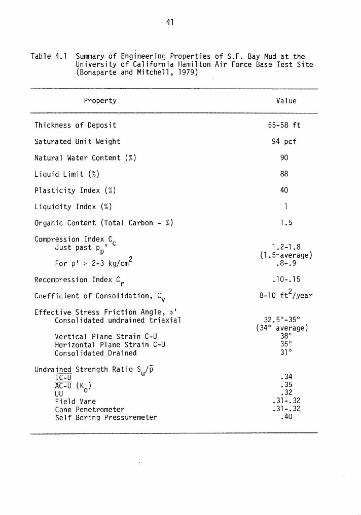
parameters are presented in Table 4.l.The laboratory effort in this thesis is directed towards the

consolidation behavior of the Bay Mud, especially as to any anisotropic

properties. Both the lateral and vertical response is needed since

drainage from the pressuremeter is influenced by both, especially the

40

4l

Table 4.l Summary of Engineering Properties of S.F. Bay Mud at theUniversity of California Hamilton Air Force Base Test Site(Bonaparte and Mitchell, l979)

Property Value

Thickness of Deposit 55-58 ft

Saturated Unit weight 94 pcf

Natural water Content (%) 90

Liquid Limit (%) 88

Plasticity Index (%) 40

Liquidity Index (%) l

0rganic Content (Total Carbon - %) l.5

Compression Index CCJust past pp' l.2-l.8

2 (l.5~average)For p' > 2-3 kg/cm .8-.9

Recompression Index CV .l0—.l5

Coefficient of Consolidation, CV 8-l0 ft2/year

Effective Stress Friction Angle, ¢'Consolidated undrained triaxial 32.5°-35°

(34° average)Vertical Plane Strain C-U 38°Horizontal Plane Strain C-U 35°Consolidated Drained 3l°

Undrained Strength Ratio SU/pIC-U .34AC-U (K ) .35uu " .32Field Vane .3l-.32Cone Penetrometer .3l-.32Self Boring Pressuremeter .40

42

horizontal response. It appears to be the first time that such an

experimental investigation has been made on Bay Mud.

Also new in the experimental program is an investigation of the

effect of OCR on the stress-strain behavior of Bay Mud. This became

necessary as the OCR in the Bay Mud is believed to vary from l to l.5.

for the depths of l8 to 5O feet where the field pressuremeter tests

were conducted. ·

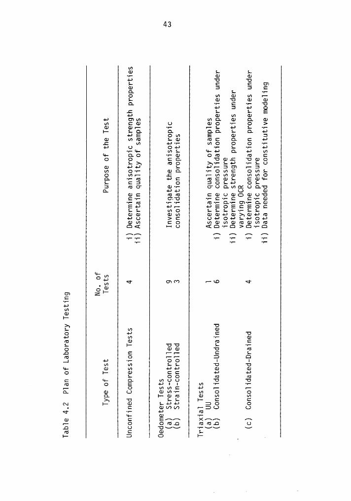
Drained triaxial tests are included in the testing program as no

such tests with volume change measurements have been reported in the

literature. The volume change data are needed in the constitutive

modeling of Bay Mud by an effective stress model. A summary of the

testing program, including a brief explanation of why each test was

undertaken, is presented in Table 4.2.

4.l SAMPLING AND PRESERVING UNDISTURBED SOIL

Undisturbed piston tube samples of 5 inch diameter were taken at

the Hamilton Air Force Base on January 25, l983. Five tubes, each

approximately l5 inches long, encased tightly in styrofoam boxes with

styrofoam popcorn, arrived in Blacksburg on February 8, l983. As

several months were to pass before the newly purchased triaxial testing

equipment was assembled, and a long duration which is required in the

testing of highly impermeable clays, it was thought necessary to

extrude the samples from the tubes in order to prevent any deterioration

of the soil (which occurs if the soil water reacts with the iron

present in copper tubes). .

WGJ L L•1- GJ GJ

4-* °O 'OL C C U?GJ 3 3 CQ L -1-O W CD W 1-L GJ 'O G) GJQ. ·•·· C •1- 'U4-* 3 4-* EC L L

4-* QJ W CD4-* OWW WQ GJ C. GJan CGJ LJ GJO *1- O >Q) GJIC -1- 1-·L 4-* L -1-I—* LQ Q QQ L Q 4-*-1-E om E GJ :GJ WFG LCD f¤C Q C 4-*L an +-*-1- I/IO O O *1-4-* U O4-* •1- L -1- 4-*•1-I4- WL '4-4-* Q 4-* WQ- Q.O *1-GJ Ofü YU CO O CC. 'OCDC 'OGJO

L>;FGOG)4-*4-* L -I-*1--DOW 1-3

W O•1- GJQ -1-OWC OWLQ an- .: «—mmGJ «.nmOQ ·1-FCS +-*C IUCGJL C('D‘4—L C3 O DOL4-* OL3 ¢'UO” GJ•I- O'OQWQf.UC."OO. 4-*4-* L) GJ(UC fUf'O CQ)OGJOGJO'O

C-- CTO ·1—C·1-C C--GJ-1- (Q •r· •1- t‘O'I- O.°!' O7°f* O.GJE4-> ·•->„- -6->EoE:Eos::LL WO LL~LL·1-LLGJGJ GJm GJGJ+-*<1J>5(IJ4—*fU+-*L) >C L)4-*O4-*L4—*O4-*GJm CQ u1GJmGJfüGJmfüC<[ I-U

IC f'\ Z'\

-1--1- -1- -1- -1- -1-

Q-¤i3U, C OWÖÖ 1-kO C

cn Z'-C-1-4-*WCUI-

'OSö W GJQ 4-* C 'O4-* I/I *1- GJFU GJ fü CL I-' 'O”O L -1-O CDG) 'O FU.Q C 1-1- C Lfü O 1-1- E C..I 4-* -1- OO l IIn In LL ‘¤ 'CJQ- CD um —+->-> GJ GJO I- GJ CC 4-* 4-*

L OO FU füQ Q- Q. I/'IUU 'U 'U„ as 0 E 4-*¤l vv '•* '•—IC O WWC 4-* IC IC¤. GJ LJ GJ•.n·•- uv O O

Q I-—GJfü GJ W W>> "O LL I·— C C

cx: I- GJ L.-1->+-> EO QQ- ·1·· 4-* YU

Q- GJ *1-IC O OVUC ¢”U*‘Ö.O O_Q Q 'QC/C4 -1-CzC4 C4FU C CD L1- D O I- ,

44

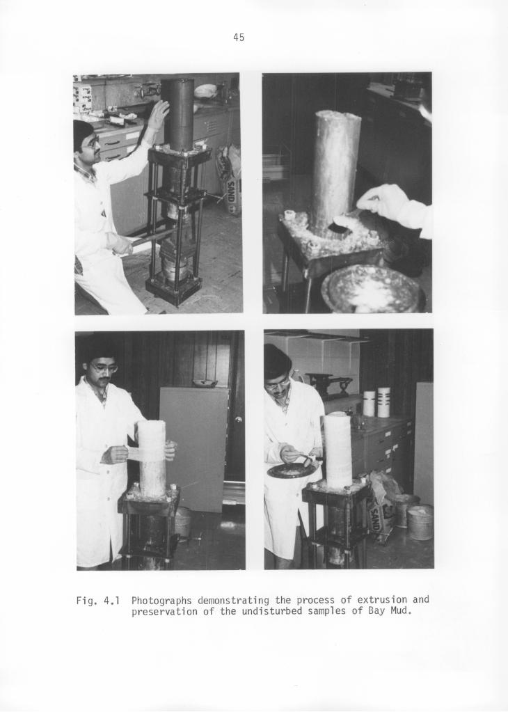
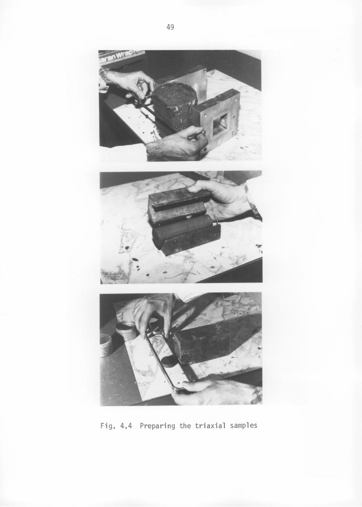
A steel extruder was designed and fabricated wherein the samplingtube could be held vertically and the sample extruded with the help ofa hand-operated hydraulic jack. The complete process is shown in

Fig. 4.l. In this essentially one-man operation, a very small amountof force was required to push the entire sample (l2 to l3 inches long)within the tube.

The extruded sample was quickly coated with a layer of melted wax

which was then covered with a single wrapping of gauze. A second layer

of wax was now applied such that the entire gauze layer was completely

soaked in the applied wax. The process was repeated with another

application of gauze and wax coating. Layers of gauze acted as a re-

inforcement providing tensile strength to wax layers.

Thus, three layers of wax reinforced by two layers of gauze

imparted enough stiffness to the cylindrical sample of soft clay so it

could be turned upside—down in hands and carried to a steel closet,incubated with a large dish of water, for storage. The soil samplesstored by this process showed no signs of deterioration or loss in

U

water content over a period of nine months that were spent in thetesting program.

4.2 UNCONFINED COMPRESSION TESTS

Two sets of unconfined compression tests were conducted on

cylindrical samples of l.4-inch (35 mm) dia and 2.8-inch (70 mm) in

height. Each set consisted of two tests: first, a conventional test,

in which the sample is prepared such that its axis lies perpendicularto the direction of the bedding planes, considered horizontal for the

46

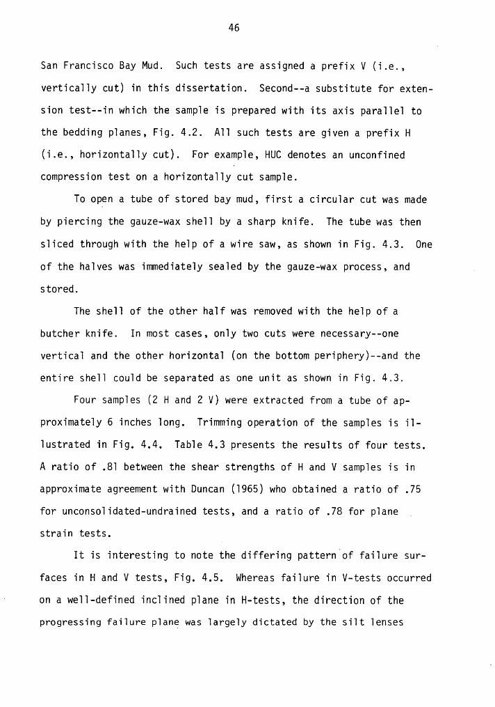
San Francisco Bay Mud. Such tests are assigned a prefix V (i.e.,

vertically cut) in this dissertation. Second--a substitute for exten-

sion test——in which the sample is prepared with its axis parallel tothe bedding planes, Fig. 4.2. All such tests are given a prefix H(i.e., horizontally cut). For example, HUC denotes an unconfined

compression test on a horizontally cut sample.

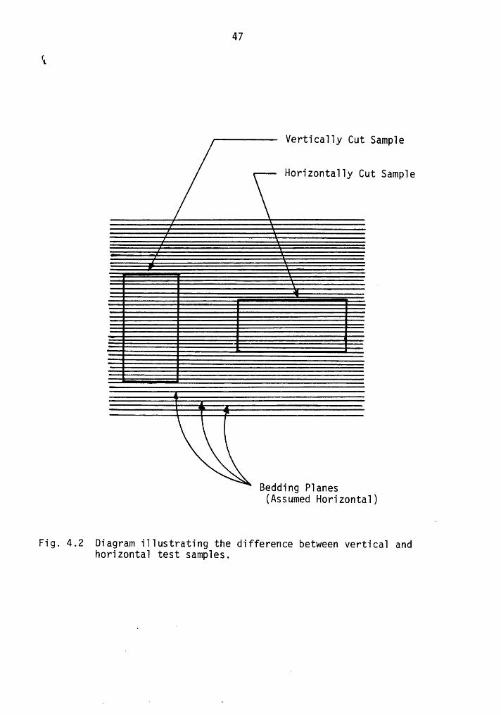
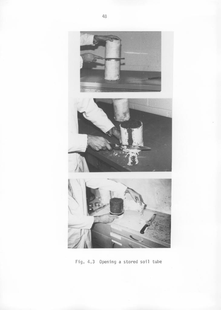
To open a tube of stored bay mud, first a circular cut was madeby piercing the gauze-wax shell by a sharp knife. The tube was then

sliced through with the help of a wire saw, as shown in Fig. 4.3. One

of the halves was immediately sealed by the gauze-wax process, and .stored.

The shell of the other half was removed with the help of a

butcher knife. In most cases, only two cuts were necessary--one

vertical and the other horizontal (on the bottom periphery)-—and the

entire shell could be separated as one unit as shown in Fig. 4.3.

Four samples (2 H and 2 V) were extracted from a tube of ap-

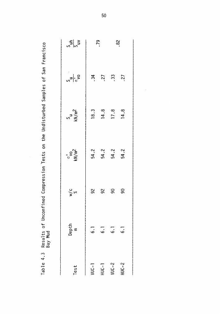
proximately 6 inches long. Trimming operation of the samples is il-lustrated in Fig. 4.4. Table 4.3 presents the results of four tests.A ratio of .8l between the shear strengths of H and V samples is in

approximate agreement with Duncan (l965) who obtained a ratio of .75

for unconsolidated-undrained tests, and a ratio of .78 for plane

strain tests.

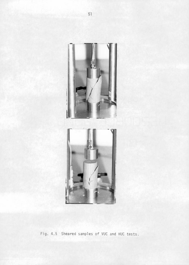
It is interesting to note the differing pattern of failure sur-

faces in H and V tests, Fig. 4.5. whereas failure in V-tests occurred· on a well-defined inclined plane in H-tests, the direction of the

progressing failure plane was largely dictated by the silt lenses

47Q

Vertically Cut Sample

Horizontally Cut Sample

=.."'*-..

Bedding Planes(Assumed Horizontal)

Fig. 4.2 Diagram illustrating the difference between vertical andhorizontal test samples.

.C > O3 C\lG : : ¤\ 00U tf) cf) •

·UI-1-UCfüL

LL.C"¤ .U3

O <‘ N (*3 N*4- 3—> (*3 C\1 (*3 C\|O tf) G ····UI**4 .I"“

Q.Efü

C/3'UGJ.Q C\I (*3 ® ® ®g E • • • •: :\ 00 <r r\ <r

-I-* (./3 Z •— r— •— r—U) x••—'UCEGJ.C4-*CO

C\| C\I C\| C\| C\IU) QE • • • •-I-) '>$ <' ÜÜU)

O Z LO LO LO LDGJ Ad,I—

CO••-tl)U)GJLQ.EO U C\lC\|L)O3 Ö3 O3 O3'UGJC

*f'**4-COUC3

*4- .CO 4-* r- r·—· •··

r—Q_E • • . •m‘¤ GJ CO CO CD LD

4-*3 Qr—·E3V*>sGJfüQSI

(*3

GJ •— r—· Q1 C\1•···· -I-J I I I I.D U') C.) L) C.) L)fü GJ E E 3 E|— I— > I > I

52

running in the vertica1 direction.

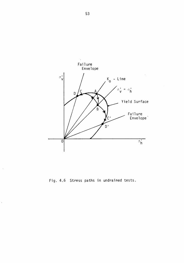
How do the stress paths compare in two cases? Stree paths for

undrained test on V-samp1es are we11 known (Bur1and, 1971). Shown in

Fig. 4.6, point A represents the in-situ stress state of a soi1 e1ementthrough which passes the current yie1d enve1ope DAD'. The yie1d

enve1ope is necessari1y non-symmetric about the hydrostatic axis,

6; = 6; for unequa1 soi1 strength in V and H tests. During the

samp1ing operation, the soi1 e1ement traverses a path AB to acquire a

hydrostatic stress state at point B.

In a V-test, the stress path rises to meet the yie1d enve1ope at

point C, and it remains on the enve1ope unti1 the fai1ure occurs at

point D. On the other hand, the undrained path for a H-samp1e fo11ows

a pattern BC'D'.

OEDOMETER TESTS

A conventiona1 oedometer test inc1udes a compression test on a

1atera11y confined soi1 samp1e whose axis coincides with the vertica1

direction in the fie1d, i.e. test on a horizonta11y cut samp1e. Such

tests are termed "HCON" test in this dissertation. An HCON test yie1ds

permeabi1ity or conso1idation characteristics in the vertica1 direction

of a stratum. Using the conventiona1 Casagrande interpretation this

test a1so yie1ds an estimate of its maximum past overburden pressure.

It fo11ows that, if the samp1e of an oedometer test is cut

vertica11y such that its axis 1ies para11e1 to the horizonta1 p1anes,

we are ab1e to obtain conso1idation characteristics of the stratum in

the horizonta1 direction. Tests on vertica11y cut samp1es wi11 be

53

FailureEnvelope

Gu KO — Line

D cAYield Surface

Failure 'C' EnvelopeDI

0 GA

Fig. 4.6 Stress paths in undrained tests.

54

called "VCON" tests hereafter. However, there is a pertinent question

in the case of this test--will the Casagrande's method for a VCON test

give the maximum past horizontal pressure? Or, could such a test

determine the present horizontal pressure in a stratum?

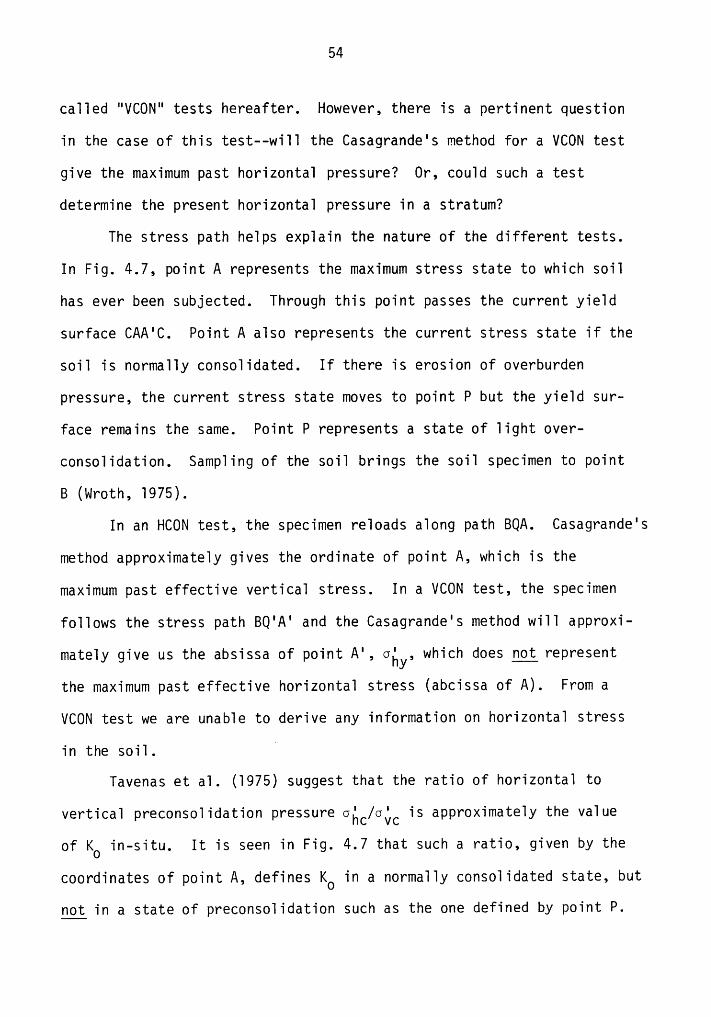
The stress path helps explain the nature of the different tests.

In Fig. 4.7, point A represents the maximum stress state to which soil

has ever been subjected. Through this point passes the current yield

surface CAA'C. Point A also represents the current stress state if the

soil is normally consolidated. If there is erosion of overburden

pressure, the current stress state moves to point P but the yield sur-

face remains the same. Point P represents a state of light over-

consolidation. Sampling of the soil brings the soil specimen to point

B (wroth, l975).

In an HCON test, the specimen reloads along path BQA. Casagrande's

method approximately gives the ordinate of point A, which is the

maximum past effective vertical stress. In a VCON test, the specimen

follows the stress path BO'A' and the Casagrande's method will approxi-

mately give us the absissa of point A', oéy, which does ngt_represent

the maximum past effective horizontal stress (abcissa of A). From a

VCON test we are unable to derive any information on horizontal stress

in the soil.A

Tavenas et al. (l975) suggest that the ratio of horizontal to

vertical preconsolidation pressure oéc/oQC is approximately the value

of KO in-situ. It is seen in Fig. 4.7 that such a ratio, given by the

coordinates of point A, defines KO in a normally consolidated state, but

ngt_in a state of preconsolidation such as the one defined by point P.

55

UIV K · Linel o

M AYield

C Surface

AI

Failure| Envelope

C' ;s ' .Ighy

O H H' 0*;

Fig. 4.7 Stress paths in oedometer tests.

GC\l

'

E GP"

LD2:.0 [ °C ' ••'ULJRO3>

'E 4:

4-*+-*>;<./7 Q •FU G) CU GJGQIPG P

LQ QEFUU)• •• O „_FUU'|‘

+->LQ)’ >

(\I FUE• •• • Q äU1

U)->ClJ0 +->

L(U-0-*Q)• •• • "' gUCDOGJ

-6->CU(_) 1---Q_ Q_

° ä...-p--.....

• ·• • LQU

<E

®<l'

• ••O[ LLI

A Q I"'

OO <l' G RO C\1 G 'C“~J C\I öl P Pc9 OILVHGIOA

57

If we compare Figs. 4.6 and 4.7, it is reasonable to postulate

that the ratio of shear strength in extension and compression is nearly

equal to the ratio of yield stresses in VCON and HCON tests.

1.e., (4.1)uc vy

An experimental evaluation of the relation (4.l) will be presented

later in this chapter.

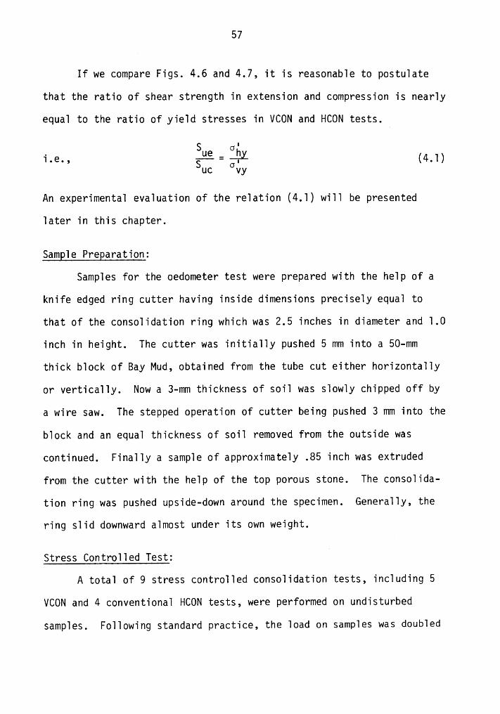
Sample Preparation:

Samples for the oedometer test were prepared with the help of a

knife edged ring cutter having inside dimensions precisely equal to

that of the consolidation ring which was 2.5 inches in diameter and l.0

inch in height. The cutter was initially pushed 5 mm into a 50-mm

thick block of Bay Mud, obtained from the tube cut either horizontally

or vertically. Now a 3-mm thickness of soil was slowly chipped off by

a wire saw. The stepped operation of cutter being pushed 3 mm into the

block and an equal thickness of soil removed from the outside was

continued. Finally a sample of approximately .85 inch was extruded

from the cutter with the help of the top porous stone. The consolida-

tion ring was pushed upside-down around the specimen. Generally, the

ring slid downward almost under its own weight.

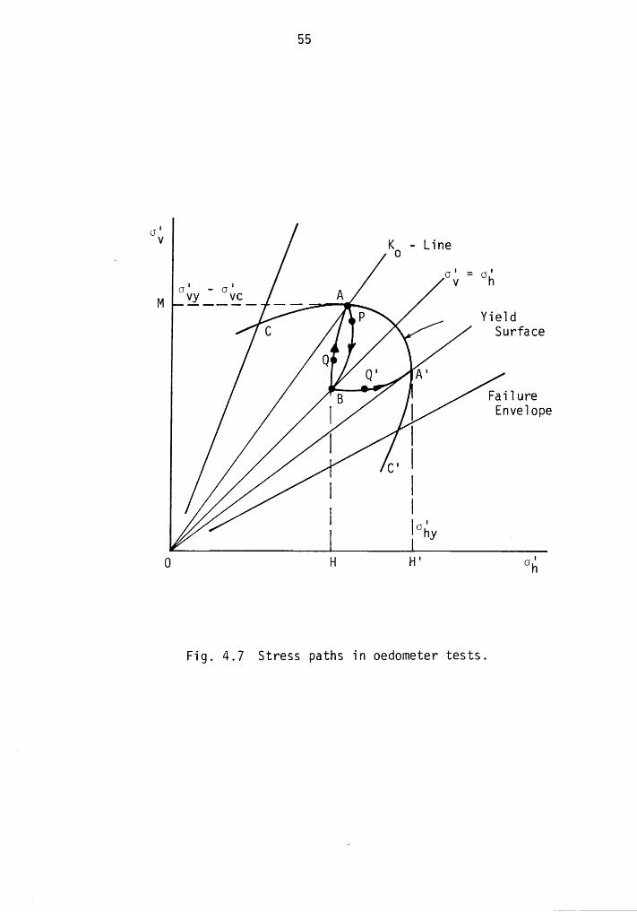
Stress Controlled Test:S

A total of 9 stress controlled consolidation tests, including 5

VCON and 4 conventional HCON tests, were performed on undisturbed a

samples. Following standard practice, the load on samples was doubled

58

every 24 hours during the loading phase. An interval of l2 hours was

permitted between successive steps of unloading or reloading. Fig. 4.8

presents a typical e-log p' curve. Curves for the other tests are in

Appendix 2. A summary of material parameters and other useful informa-

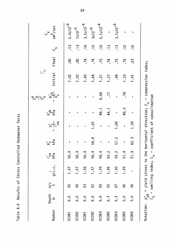
tion that could be derived from the tests is given in Table 4.4. An

average value of 0.8 for the ratio of yield strengths in VCON and HCON

test provides an encouraging evidence to the validity of Eq. (4.l).

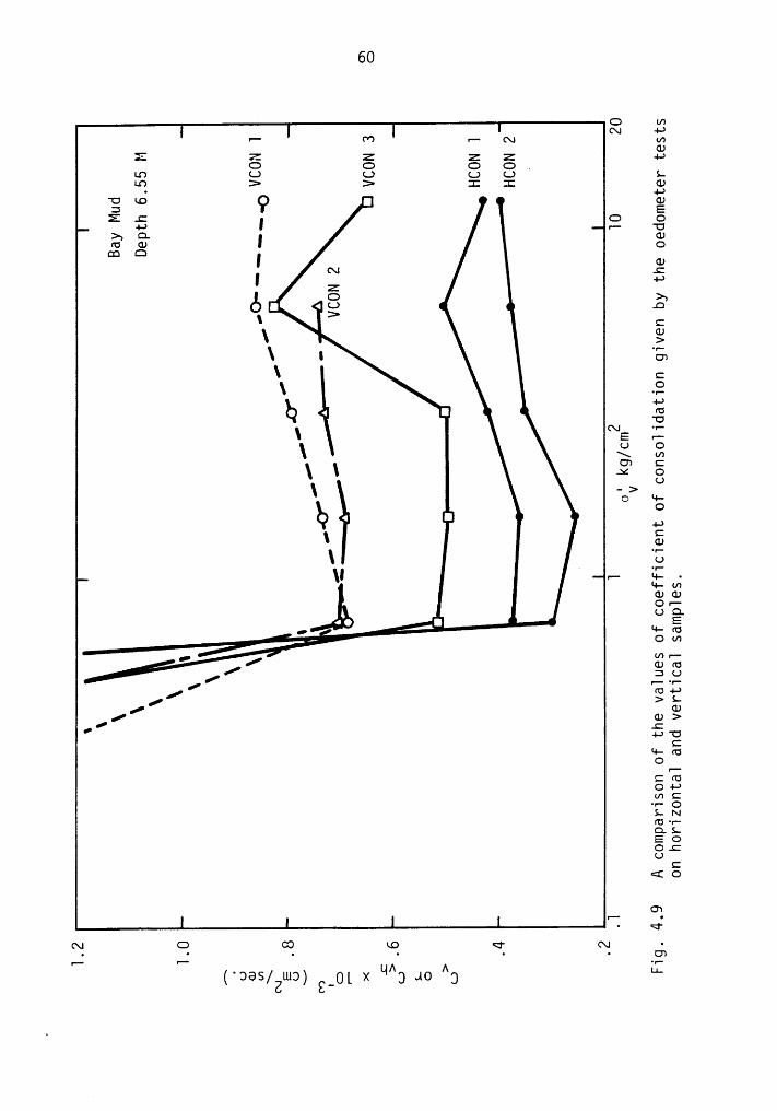
Fig. 4.9 demonstrates a comparison between the values of the coef- (

ficient of consolidation for Bay Mud in horizontal and vertical direc-

tions. A value of 2.5 is suggested for the ratio Cvh/CV in the

normally consolidated zone of Bay Mud.

Strain Controlled Tests:

A considerable amount of time is required for performing a con-

T ventional stress—controlled test. Even then, only a handful of data

points are obtained for an e-log p' plot, and thus, the test requires

a subjective judgement in the determination of preconsolidation pres-

sure. However, if the specimen in an oedometer is compressed at a

constant rate of strain (CRS) slow enough to dissipate all excess pore

pressures in the specimen, just like in a drained triaxial test, a

continuous plotting of the e-log p' curve can be made within a

relatively short period (l to 2 days) of time. This allows an accurate

definition of the preconsolidation pressures. Tests of this type by.

Denby (l978) led to preconsolidation loads higher than those of con-

ventional oedometer tests on Bay Mud.

Ü Ü Ü ÜU I I I I(U O Ü O Ü O OU) IÜ I IZ I IÜ I-·

> \ X O X O X I X I IR.) C\I Ü IZ LO r- I- F1

E• X • X • •

U LO N (*7 O') LO O')

(*7 (*7 RO LO O (*7 (*7 AI ROU) IZ IZ IZ I- IZ IZ I··— IZ I-

Q • • • • • • • • •

!"'fü O O Ü Ü Lt') Ü LO RO O')c GO GO Ix IL Ix Ix I\ I\ RO ••·

I I I I I I I I

ILI. (UE·L) „,..L) ,.

fü (\I (\I LO Ü IZ N Ü Ü I- C'I" O O Ü RO (\I (\I O) (\I O) O+.7 • • • • • • • • • •|—•I— I- I-- IZ IZ IÜ IÜ IZ fl (/7C U)>-• GJ

LQE.: <I· r\ GO O— -U (Ü N N U C(D slu 3 Q Q I I I I • • I • I O

L/7 U') O II ·I-II -I-*U fü

L7 'O•I-IZ I- (*7 ••* ft

_c (U • • • C O->,¤. I I I I GO <r I GO I 0 InIn Q AC Ü Ü Ü •I- C

-I-* -9 OIn U UCU GJI- O IÜ RO O L '~I--U·> O O C\I •I·- OL Q O I I I • I I • I • 'OQ) FZ Ii IZ -I-—*+-* II IÜ CQ) fü (DE 4-* •I-O C U

'O O7 C\l (*7 O •I-Q) (U • • • ‘ Q-O -U¤. I I I RO I I N I C\.I ·I- I4-

O. A4 Lt') LO RO L (D'O O OG.) .C UIZIÜ Ü Ü Ü Ü Ü (\I GI O) O) C1) IIO . Q (U • • • • • • • • • _C

L —>O- RO RO RO RO RO Ü Ü IÜ IÜ +-* >-I-* O A6 Lt') LO Lt') Lt') LO LC) Lt') Lt') LO OC CO nl- nß

Q,) X• U1 Q}U) U N N G7 N O) RO O C7) U) 'OU) • Ü Ü Ü Ü Ü Ü LO Ü G) CQ) • n • • • • • • | L •I-

L L I- IÜ I- IZ IÜ I- I- IZ -I-*4-* O) U) O')L/7 C

'O •I-RI- I··· IÜO U (D fi

Nä (*7 (\I O LO N RO RO •I·- Q)U) E O) O) O) O) O) O) O) O) N 3-9 U)IÜ II3 IIU) .C .CQ) -I—* RO RO RO RO RO I- IÜ RO RO ··N U)E n • • • • • • • • Q_

UG) RO RO RO RO RO RO RO L.') LF7Oq- „

• CÜ O

L •I·-Q) Q) IÜ C\I Il C\I (*7 Ü (*7 LO Ü -I—*Ii .O Z Z Z Z Z Z Z Z Z fü.Q E O O O O O O O O O -I-*fü 3 LJ O O O C.) LJ C.) C.) (.7 OI- Z > > I I > > I > I Z

60

O an

m 3 3 3 3~ LLQ > > :1: :1: Ä]

‘0 LO2 2 ‘•° ' E4-> I 0 0

>, Q.•— U

¢¤ cu I cuE 2 I

OGJI ‘“‘ =

ä P60‘>‘ §

\ I*1-‘ 05

\ COE

l «¤"ON •‘ E S

\ 3 ¤I cn

AC Q

\ ->U

O 9-

Ö · °-6-*

\ s:GJ

\ ‘*‘U\| ,.. 1;:,L1-mCDG)@|—

_;’ :2FG’/ :0

!*"!*@4-*>L„

ffGJ

0g>4->‘O

CqöföCTO04-*(DC•P¤O

LNFUN-0.LE0

C<E0

OWfi O

C\I

l qr

u-—· p- ° '• Q7

. A A*•·—

(DBS/ZLU3) X L4 UJQ 3 1.1..

6lA total of 4 CRS consolidation tests were run during this testing

program on Bay Mud including a test each on undisturbed HCON and VCON

samples and two tests on remoulded Bay Mud at different strain rates.

Drainage was permitted at the top and bottom of the specimen.

Constant rate of loading was applied through a hydraulic frame. _

A newly acquired electronic data acquisition system was used for con-

tinuous recording of the applied load and the change in height of the

specimen. Load was measured by a 2000 lbs. load cell and displacement

through a Linear Variable Differential Transformer (LVDT). Micro-

computer program was designed in such a way that it recorded data every

5 minutes for the first two hours, and every l5 minutes thereafter.

A complete set-up of the test equipment is demonstrated in Fig. 4.lO.

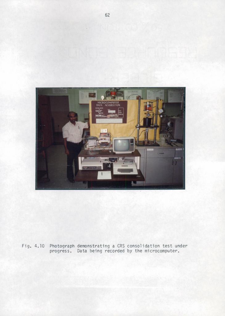
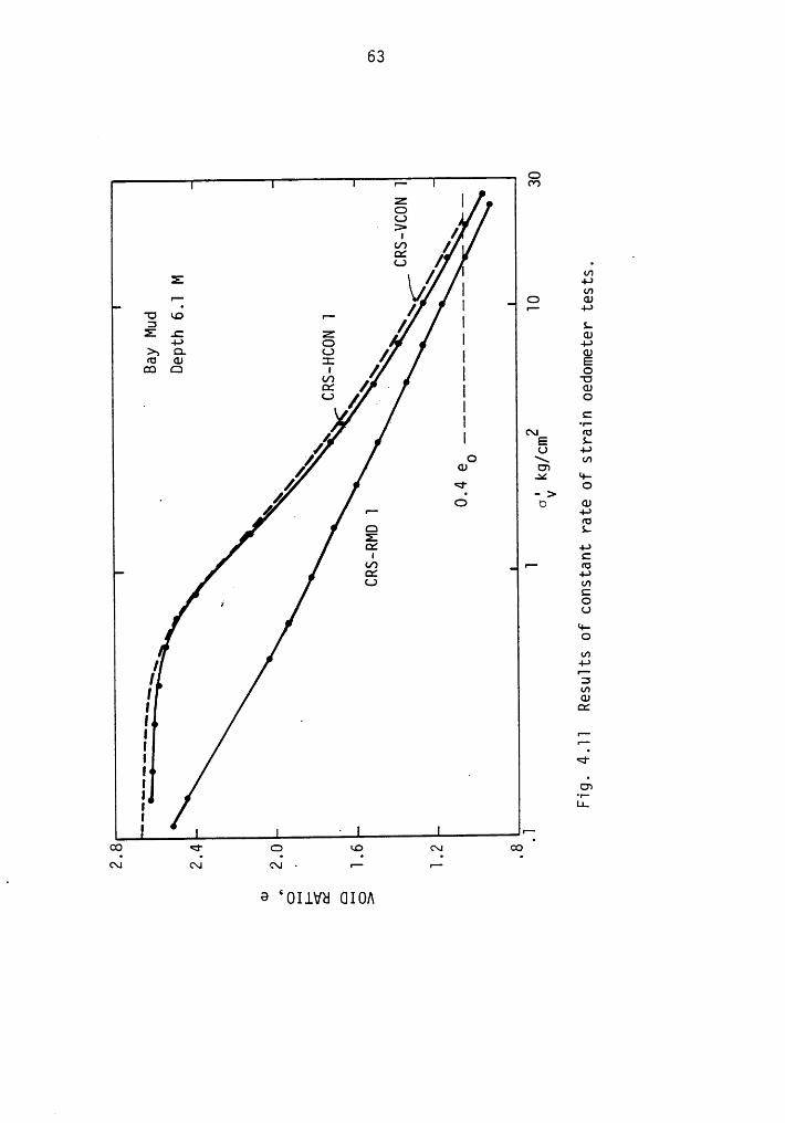
Fig. 4.ll shows e-log p' curves for the CRS tests. The plot

gives an overconsolidation ratio of l.3 against a value of l.06 noted

for the conventional test for a depth of 20 feet. However, CC values

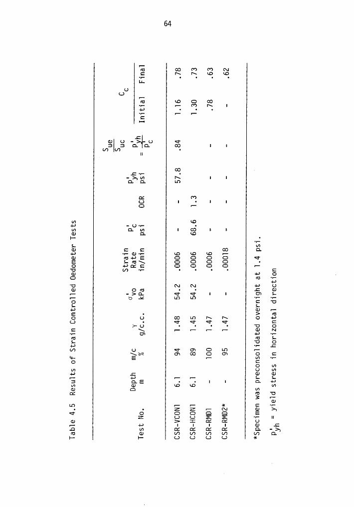
are similar to those obtained from the conventional test. Table 4.5summarizes the results of the CRS tests. A value of .84 is obtainedfor the ratio of yield stresses in the horizontal and vertical direc-

tions which is again comparable to that obtained from the conventional

test. Variation in strain rate in two CRS tests had no effect on thecompressibility of remoulded Bay Mud, as seen in Table 4.5.4.4 TRIAXIAL TESTS '

In order to determine stress-strain strength parameters, drained

and undrained triaxial tests were performed on undisturbed samples.

During the consolidation phase, careful measurements of volume change

63

C)r-· (*7

Z IO6 SI //U')Z .L.) /

I•

In

ri [IE“° Z I „.E .C Z /

I G)-0-* ® -I-0>„ Q. C.) / I GJFU CU I EQ Q I [ I c

tf) U2 'I I 2. / M I C. I „_

/ I N5 fs?..' 2 2 2// Q) U7x I+-/ <¤j ¤’ / G

-O> GJ/ I- -I->ruQZ L°f E"' EIUj

OUH-OIn, -I->

{ EQ)[ QtI .I F"

I '"ZI <rI - .I .9| L1.I Ä I-

00 <r Q ao cx: oo•

GI (\I GI ·•— s-

6 ‘01Iva GIOA

P(U CO (*7 (*7 C\IC N N LO LO

I I l O

LJ.U

LJPf¤ (O G G•r- P (*7 N I+.7 • • 5°f* IC IC

CI-•

-CGJ U - U Q: Q Q. Q. 00 I Itf) U') •

ll

.O

- >~, UI N I IQ. Q. LO

(*7(.7 I • I IQ P

In RO4-* - L) •I-

~In Q. In I CO I IGJ Q. SDI- •

•I-L U7(U C C G O.4-* ·r· GJ ·¤— LO kD (D Pcu ru -I-> E C> CJ CD c <I·E S- IG \ G G G G •O 4-* M C G G G G P'¤ (f) •y-• • • • • C(U 4-* O .G •'¤ •r-

4-*'O C\| (\I 4-* UCU O ¢‘¤ •

· -C GJP • > Ü. I I G7 LP O X LO LO ·r· •r-

O C CS- L

4-* GJ PC • > IGO U G LO N N O 4-*G • Q Q Q Q C

>- U • • • • '¤ OC N P P P P CU N'f' CD 4-* •r-(U (U LL 'U O

4-* •v·· CU7 U OG LO P

OW G O7 O C'~I— E P L/7 •r-O C

O UIL/I U I./7

4-* C GJ (DP 4-* P P L L3 Q. E •

· I I Q. -I->m QJ (O LO InGJ G V7Of (U 'O

3 P(U

LO P IC 'X C °|*• • Z Z IC GI CL) >3Q O G G G G Ez c.: U Z Z ··— IIC1) UP 4-* I I· I I CU C.Q In M M M M Q. - >„(U (1) (./7 (/7 (/7 (/7 C/7 O.I- I- U <.> c.: <.> -I<

65V

versus time were made which enabled the determination of flow charac-teristics of Bay Mud under isotropic stress. And thus, as a byproduct

of the triaxial tests, it became possible to provide a check on the

value of horizontal coefficient of consolidation obtained from the

oedometer tests. An advanced triaxial equipment is needed as volume

change measurements have to be made under back pressure.

UU Test:

One unconsolidated undrained test was performed which gave a

SU/pé ratio of .33, almost equal to that of unconfined compression

test. A failure strain of 6-7% was noted.

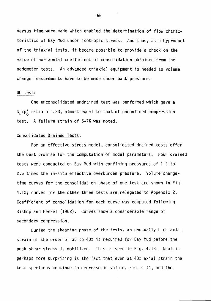
Consolidated Drained Tests:

For an effective stress model, consolidated drained tests offer

the best promise for the computation of model parameters. Four drained

tests were conducted on Bay Mud with confining pressures of l.2 to

2.5 times the in-situ effective overburden pressure. Volume change-

time curves for the consolidation phase of one test are shown in Fig.

4.l2; curves for the other three tests are relegated to Appendix 2.

Coefficient of consolidation for each curve was computed following

Bishop and Henkel (l962). Curves show a considerable range of

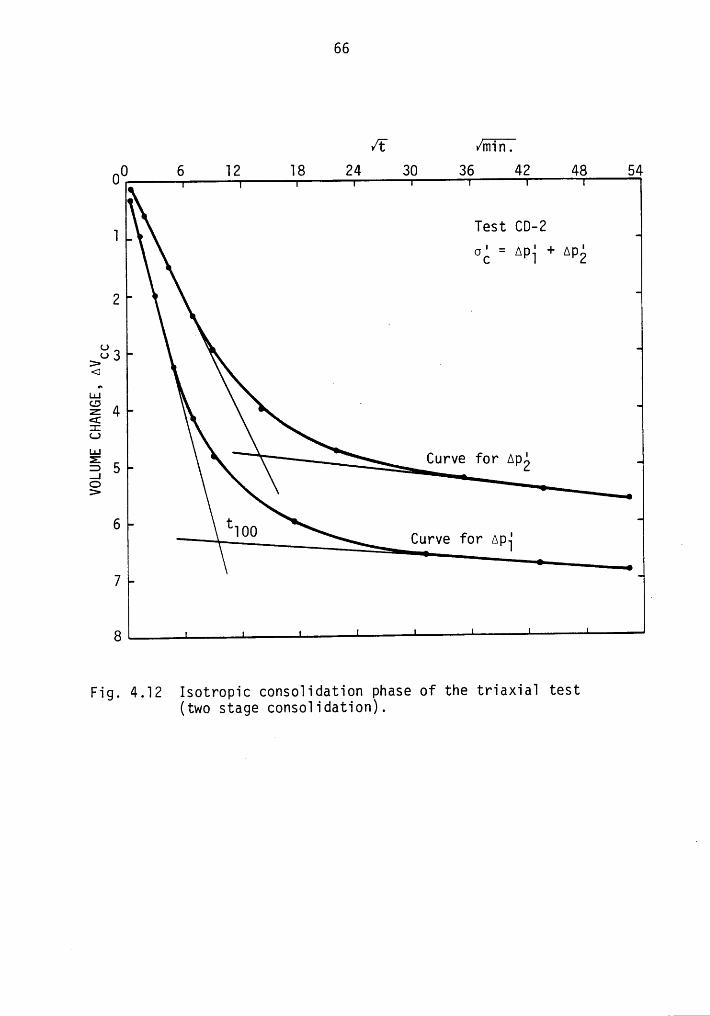
secondary compression.During the shearing phase of the tests, an unusually high axial

strain of the order of 35 to 40% is required for Bay Mud before the

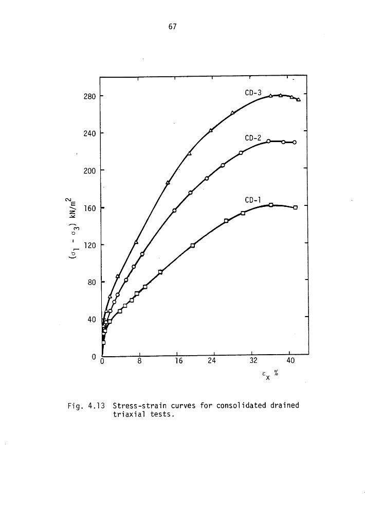
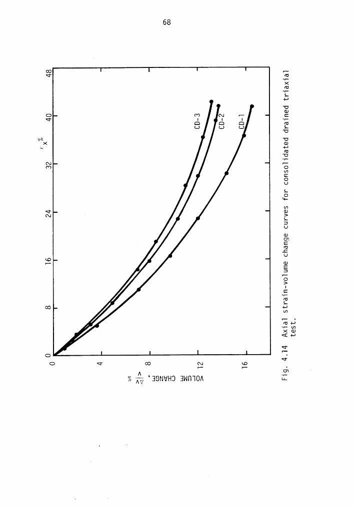
peak shear stress is mobilized. This is seen in Fig. 4.l3. what is

perhaps more surprising is the fact that even at 40% axial strain thetest specimens continue to decrease in volume, Fig. 4.l4, and the

66

ft /min.00 6 12 18 24 30 36 42 48 54

1 Test CD-2°é ‘ Api + ^Pé

2

<ä .gg 4Iga

5 Curve for Apéc::>

6Curve for Ap1 1

7

8

Fig. 4.12 Isotropic conso1idation phase of the triaxia1 test(two stage conso1idation).

67

280 CD‘3 · · . _

240 ‘ CD_2· • •

200 2 · °

~ 00-1 2§ 160 . _ ' ·.>£[T"')

O'_ 120 ‘-fl • 0

80 A ° _

40 ,!.

0 0 8 16 24 32 408 %X 0

Fig. 4.13 Stress-strain curves for c0ns01idated drainedtriaxia1 tests.

68

* r—Q FU

°I*

><FU'|“

L+-9

EC\.l r— CQ 1 1 1 -1-E Q Q FUL.) LJ C.) L

'O

ku +-9FU

'O'I*

% ICOU)COULO

- '+—In

ÄÜ S EL3UGJC7

· CE

ko UF" GJE3

|'*

O>IC

°|"

E@ -I-9

U')

·FU -I-9/ ·1· I/7

>< CD<E 4-9

QÖQ

CD Q ® C\| SO

o EISNVHI) HNÜWOA Lg

69

critical state condition, in a true sense, is never attained. This is

due to a highly compressible nature of the Bay Mud.

The stress-strain data for the drained tests is documented inAppendix 2. Test data has been corrected for filter and membrane ef-

fects following the recommendations of Duncan and Seed (l967).

Consolidated Undrained Tests: gDenby (l978) conducted a series of undrained triaxial tests on

Bay Mud following the SHANSEP approach of Ladd and Foot (l974) wherein

the samples were anisotropically consolidated with an assumed value of

KO. Similar tests had been reported by researchers at Berkeley

(Bonaparte and Mitchell, l979), but what distinguished Denby's test

was his use of back pressure of an order of 95 psi to ensure the

complete saturation of samples. while Denby found the same order of

ultimate shear strength as those of previous researchers, a conspicuous

decrease in the failure strain was noted. Denby's samples failed at

approximately 2% axial strain as against 4 to 6% reported previously.

This resulted in an increased value of shear modulus.

Undrained tests in the present investigation were conducted on

isotropically consolidated samples with a back pressure of 90 psi. The

stress state in all samples was brought initially to the virgin con-

solidation line through a consolidation pressure of at least l.5 times

the in-situ overburden stress, and subsequently unloaded to induce

0CR effect if desired. Values of l.0, l.2 and l.5 are used in the

tests. Appendix 2 includes results for the undrained tests. Table 4.6

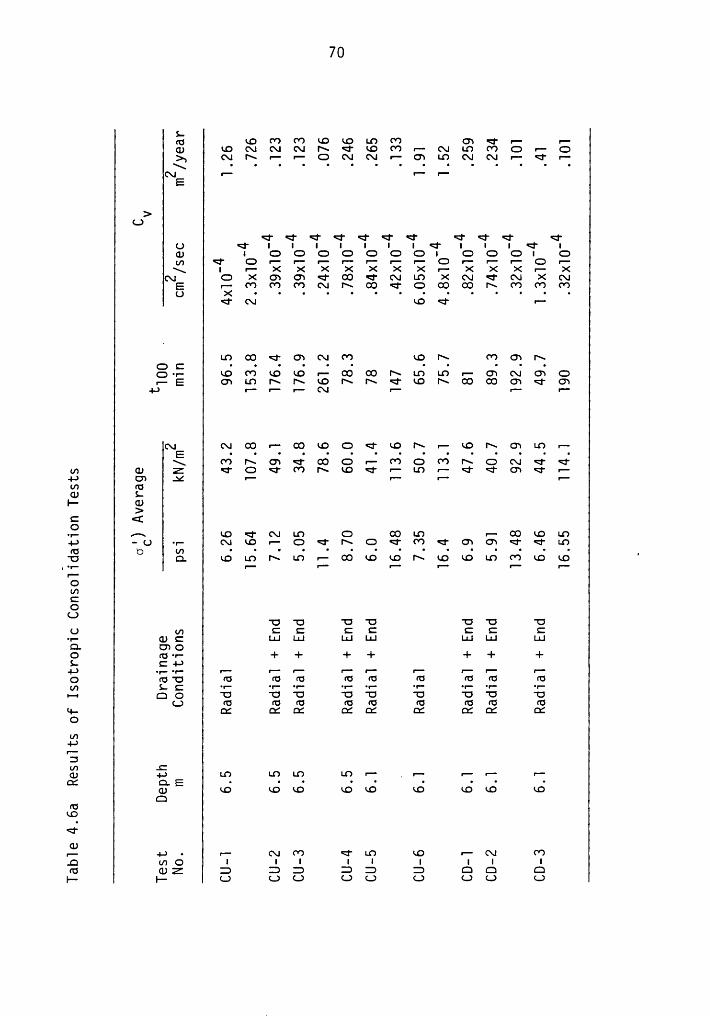
Lfü RO (*7 (*7 RO RO LO (*7 C7 C IC 1-Q) RO (\I (\| (\I N C RO (*7 IC C\I LO (*7 G IC Q(\I N IC IC G (\I (\I 1*- C7 LO (\I (\l 1- C I"-

I I I I I I I I I I I I I I IQ] IC 1- IC

E

>L)C C C C C C C C C C C

0 <r 1 1 1 1 1 1 1 <1· 1 1 1 <r 1q) 1 CD O O O O O GI O O O1 C)gn C G IC 1- IC 1- FC IC IC G IC 1- IC G IC\ I 1- X X X X X X X IC X X X IC X(\I G X C7 C7 C C (\| LO X (\.| C AI X (\lE 1-; (*7 (*7 (*7 (\I N G C G G7 G N (*7 (*7 (*7U

• • • • • • • • • • • • • •C GI RO C 1-·

LO C C7 C\I (*7 RO N (*7 ON NO:

I I I I I I I I I I I

@-1- RO (*7 RO RO IC N LO LD FC ON (\IC71-EG7 LO N N RO N N C RO N G G C7 C C7-|-7 1- 1- IC (\I IC IC IC

C\IE (\| 1** CO RO G C RO N IC RO N ON LO 1--\ (*7 N C7 C G G 1- (*7 G (*7 N G (\I C C

an (D Z C G C (*7 N RO C FZ LO 1- C C C7 C IZ-|-7 Q') _¥ IZ 1- IC 1-U'1 füGJ LI- G)

><[-1- r- RO C (\.| LO G G LO 1- G RO LO4-) •O ·1- (\I RO IC G C N C (*7 C O7 C7 C C LO¤ Ö I I I I I I I I I I I I I I I

IU Q RO LO N L.O IZ G RO RO N RO RO LO (*7 RO RO1*1- IC 1- IC IC 1- FC1-OL/ICOL)

U U U U U U UU m C C C C C C C

-1- Q): L1.! L.1.| L1J L1.! L1..| L1J L.1JQ O7OO ¢‘ü•1- + + + + + + +L C4-)

4.) 11--1- 1- IC IC 1- 1- IC IC IC 1-O füU fü fü fü fü fü fü fü fü füm L; -1- -1- -1- -1- -1- -1- -1- -1- -1-

1-1 go U U U U U U U U ULJ f‘ü fü fü fü fü fü fü fü fü

N- 1 1 G5 1 1 1 Of. 1 OCO1./'14-)

FC3Ln .CQ) «|-7 LO L(7 LO LO !*' _1- IC 1- FC1 ¤_E . 1 1 1 1 1 1 1 1

Q) RO RO RO RO RO RO RO RO ROCDfü

ROCGJ 1IC 4-* • 1- A1 (*7 C LO G FC (\| (*7.¤ 1.nO 1 1 1 1 1 1 1 1 1fü (DZ G ID D Z7 IJ 3 G G GI- I- L7 L7 L7 L7 L7 (.7 (.7 L7 LJ

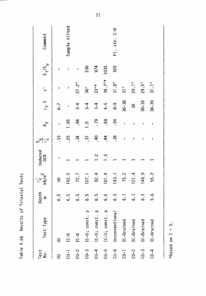
'UGJ E+9 I

+9 1- (.7C "" .(D 49 ·E S-E (D +9Q 1- (/7

L7 O.E •(U 1-

(/7 Q.

3(/7 O Q' L(7 LO\ 1 1 1 M N M CD•1- LO C7 LOL|_|

1--

-I<O 0 O 0 0 O(\I -I¢ N ä IZ LO 1-

.. [ | • O Q • • O • • •

6- N (D (*7 <I' 1- 1- CD ON Yi(\I (*7 (*7 (*7 (*7 (*7 (\I (\I (*7

N C7 C7N ä' <' <' LO O3 (*7 (*7 (*7#-1- 1 1 1 1 1 1 1 1 0,.) 1‘ 1

(.1) (D (*7 (*7 (*7 ä' @ (O G] ®(*7 (*7 (*7

LO (O C7 ® <'I1- | G G7 O N (O ON I I [ I<

• • • • • •FZ IZ

(*7 LO §' N <I' (OJI- U M N M M Q- Q- M 1 1 1 1• • • • • • •

"UCU .(JGS (\I LO3(J I ·

•IZ 1*- IZ F- fi r'- I'- ft IZ 1-

C1-1

42 (\.IE G N IC <I' <" 1- C\I ä' G7 (\IV7 ‘ UN E (\.I (\I N (\.I 1- (*7 LO fi LOGJ O Z E d' N C7 <‘ N C\I LOI- X Ii 1- fi IZ IZ 1-

1-(U•'—¤

IX +9 LO LO LO LO LO LO LO IZ IZ fi LO

Q O O O O O O O I l O Q

-1- (1) LO (O (O (O (O (O (O LO (D (O LOLI-

I-I-O D. D. Q. 1-

FU• ••+9

(U +9 +9 +9 OIZ O. (/7 (/7 1/I ·1— 'U 'O 'U 'U3 N C C C -I-7 (U (U GJ (IJ •U') I- O O O C C C C C OQ) L) L) L) GJ 'I- -1- -1- •1-Qt +9 > (U fd (U (U II

U-) 10 ••~ •n C L L L LG) E E E E E O 2 L7

.¤ I- 1 1 1 1 1 U 1 1 1 1(D E (.7 (.7 L7 (.7 (.7 C (.7 (.7 L7 L) C

• 1-1 1-1 1-1 1-1 1-1 1-1 1-1 1--1 1-1 Qä' TJ(D GJ

PC +9 _ YZ (\I (*7 <I' LO (O IZ (\I (*7 Q' m.O (/7 O I I I I I I I I I I tt}f¤ (IJ Z ID D D 3 3 ID E Q Q Q Q LDI'- I- E L7 L) (.7 (.7 L7 L7 LJ (.7 (.7 (.7 -)<

72

summarizes the useful information extracted from all triaxial tests.

Failure strains again appear to have reduced to 3 to 4% as against 6

to l0% reported previously. Such reductions in failure strains are

attributed to the use of back pressure. Again, a critical state for

excess pore pressures is seldom reached.

Determination of initial tangent modulus, Ei, from undrained

stress-strain curves is a tedious task and is often subjective. For

heavily overconsolidated London clay, practice has been to assume the

value of Ei as the secant modulus at l% strain (wroth, l97l). An

unrealistically low value of the modulus is obtained by applying such

technique to soft Bay Mud. Denby (l978) obtained the Ei values of Bay

Mud by fitting initial portion of the undrained stress-strain curve as

hyperbola. Procedure is illustrated in Fig. 4.l5. Values of Ei/SUwere obtained as high as 2500 which appear to be unrealistic for soft

clay like BayMud.In

this work, a new procedure is devised for the determination of

initial tangent modulus. The technique lies in plotting the secant

moduli of the earlier portion of the stress-strain curve against the

corresponding axial strains on a semi-log plot, as shown in Fig. 4 I6.

Extrapolated value of the secant modulus at zero percent strain is the

initial tangent modulus for the test. For normally consolidated Bay

Mud, an average value of 520 for Ei/Su ratio is determined by the methodwhich is in close agreement to a value of 600 suggested by Fig. 4.l7, ·

due to Duncan and Buchignani (l976).

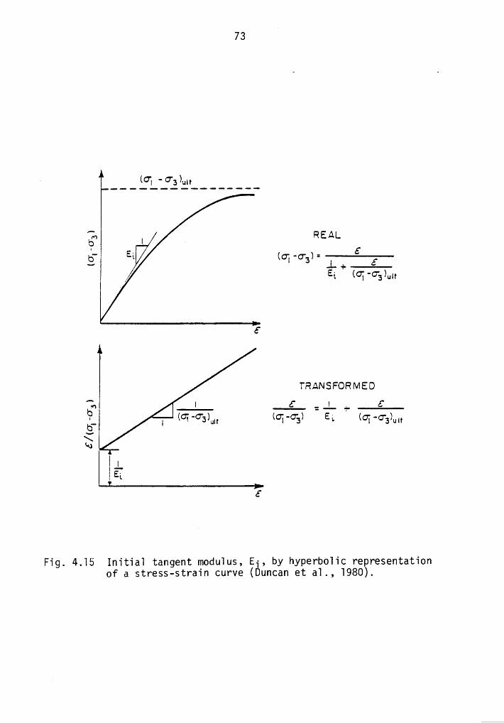
73

.. - - i°L‘.°’2’2*........

E i _ REALP:

Ea •g·3) =.—+E1 (Gi ·¤31„n

E

TRANSFORMED1 4. 4 , L . 4.E, i*91i'

*0

LEaE

Fig. 4.15 Initia1 tangent modu1us, Ei, by hyperb01ic representationof a stress-strain curve (Duncan et a1., 1980).

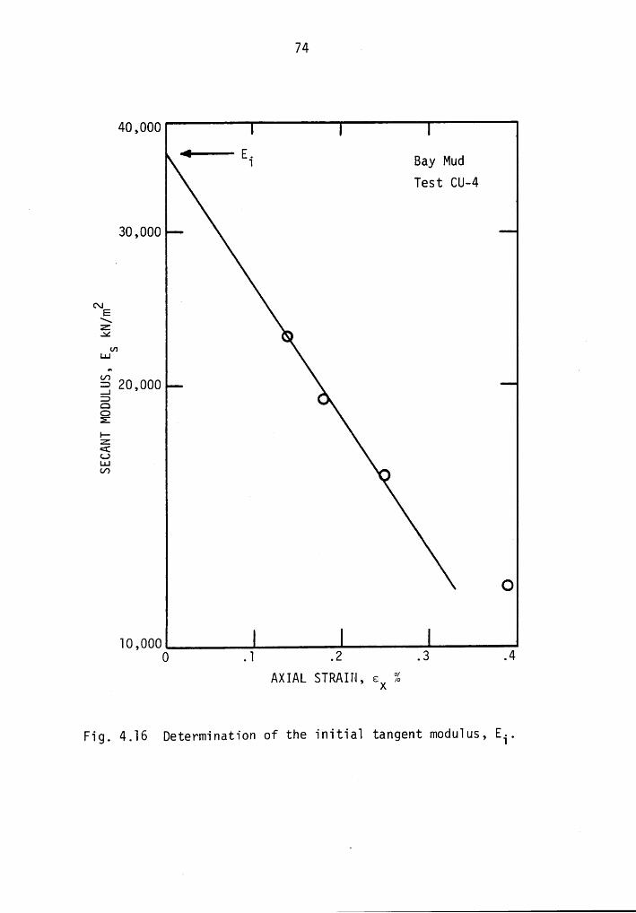
74 «

40,000

Ei Bay MudTest CU-4

30,000

-E\Z

anLLJU; .; 20,000Q OCJZf;EELJLu”° •

O

10,0000 .1 .2 .3 .4

AXIAL STRAIN, ex %

Fig. 4.16 Determination of the initia1 tangent m0du1us, Ei.

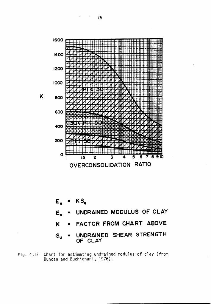
I 75

1600 11$—_IIIIIIIIIIIIIIIIIIIIIIIIIIIIIIIIIIIIIIIIIIIIIIIIIIUIIInnnununnueeeeeeeeeeuen 11ee eeeeee11e1111111 11111Zä2!1ä§ä2!!111n1111•n111h1• 1„111•11111111I 111*31111

|4OOr4z•u•4•4•nen.~ee eu 1 1111 eeeee 111111111 II n1 1 II—Zh-ZIIIIIQIIICIIIIPIIIIII uns IIIIIIIIIII IIIIIIIIIIIIYAIICVAIIIIIZIKIIGQQI nu uh e Ilullllllllll IIIIInunnuuzuneueeneunes J I1 eu! II Inu 1I uu 1 11200 2111'2!1i1111111111111:Z 1„I1111•1111„«111•1n1111IIIIn1n"·‘· ·

‘ . ”°zF I2ää2!}1111111111111111„f•1111'11•11'1E1I 111111 III2äi‘$2?1F1!1111!11!111111!'i'1IIE111lih' '1'11II111' 1Eé==é··i:€::·=£11é:a:‘::=‘:::‘E;=:·.IäII··:E§I1"·ä4 .1* ' L . 2 2 Z -znugnnennuezece ee¤•1m1•:1g1¤,u äluhm

1K 800 1121}$.'1111111111111111a1!1111111111T hh%2Z11§$111111111!1111§1!111111I111111!1II IIIIII1

uzguemrepneneeneeseg 211 1111:,, neuem II 1 1600 nu 2•z•4g4en•ueue•.11m1•41 queneen 1 u11£1§11'§§&$;¤§1€'”!'11111'111'1I1'1i111111111I*111111111II"II1'1n‘n-“

: ' 2 . I ·::7 ' Ü . ' Ü ' Ü. 1ääääääääää11111«12!1=1·'.1111I1111111111111111n!1IIIIEIIIIIIa1:.•·•e•=1:11¤•e.1e•1o>>·>>·m¤.vg•1 veeneezsezngeaeunäy-.· py

400 sa-Inn 1eu¤.ee.4„4¤«c««m„n ••neue „ee.•1•:• ..111•..·¤r•e see .111 .n111:«I11e1111-•4•.-.-;:—·~¤·o:1m¤:·2mzanssezasussaszaassnrO

1'ZI'II'_F)PlIPlI5II%II•••.'"!Iv)¢0§lX¢0)9))D10C¢¤·„7"|I nm29 zuu1v•e~•.•.¤zeeneuemmeecu, ~··¤o;assssssmass:z1n.:··v.••1•¤¤¤ee•1••11e•4ezeez•e••1em1••Ien•. :—¤2za1¤ss:¢¢1sw:«::-;n------.-„„....-;; ·-·-•1¤211g!g_;=!=ee¤ee„.é::·;·¤:11aggggggggg==lll11"'111'11111I111111···•1 ‘11‘12'!=!1!=*¥*==¤1¤··-•O 1111$$—mIII!Ill IIIIII„IIIgllslllalalllihlllllllllll

I I.5 2 3 4 5 6 7 8 9 IO ·OVERCONSOLIDATION RATIO

•Eu KUNORAINED MODULUS OF CLAY

K • FACTOR FROM QHA RT ABOVES„ • UNDRAINED SHEAR STRENGTHOF CLAY 1

Fig. 4.17 Chart for estimating undrained modu1us of cIay (fromDuncan and Buchignani, 1976).

’

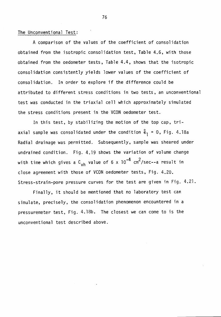
76

The Unconventional Test:‘

A comparison of the values of the coefficient of consolidation

obtained from the isotropic consolidation test, Table 4.6, with those

obtained from the oedometer tests, Table 4.4, shows that the isotropic

consolidation consistently yields lower values of the coefficient of

consolidation. In order to explore if the difference could be

attributed to different stress conditions in two tests, an unconventional

test was conducted in the triaxial cell which approximately simulated

the stress conditions present in the VCON oedometer test.

In this test, by stabilizing the motion of the top cap, tri-

axial sample was consolidated under the condition @1 = 0, Fig. 4.l8a

Radial drainage was permitted. Subsequently, sample was sheared under

undrained condition. Fig. 4.l9 shows the variation of volume change

with time which gives a Cvh value of 6 x l0-4 cm2/sec--a result inclose agreement with those of VCON oedometer tests, Fig. 4.20.

Stress-strain-pore pressure curves for the test are given in Fig. 4.2l.

Finally, it should be mentioned that no laboratory test can

simulate, precisely, the consolidation phenomenon encountered in a

pressuremeter test, Fig. 4.l8b. The closest we can come to is the

unconventional test described above.

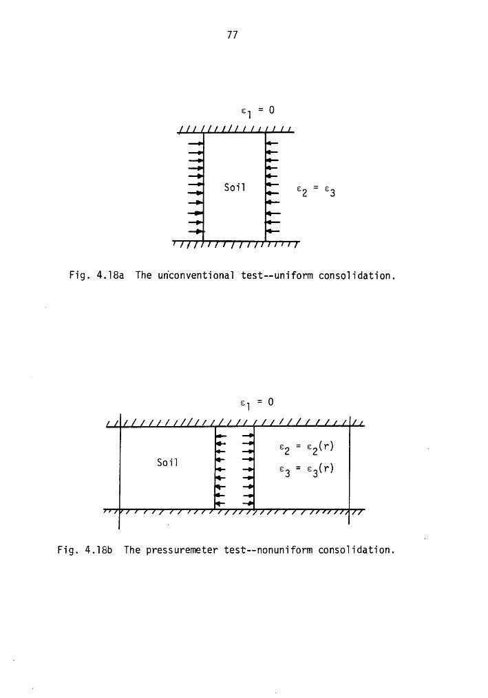
77

61 = O/

Soil 62 = 63

Fig. 4.18a The udconventionai test--uniform consolidation.

€·| = 0/ / /

62'

/

Fig. 4.18b The pressuremeter test--nonuniform consoiidation.

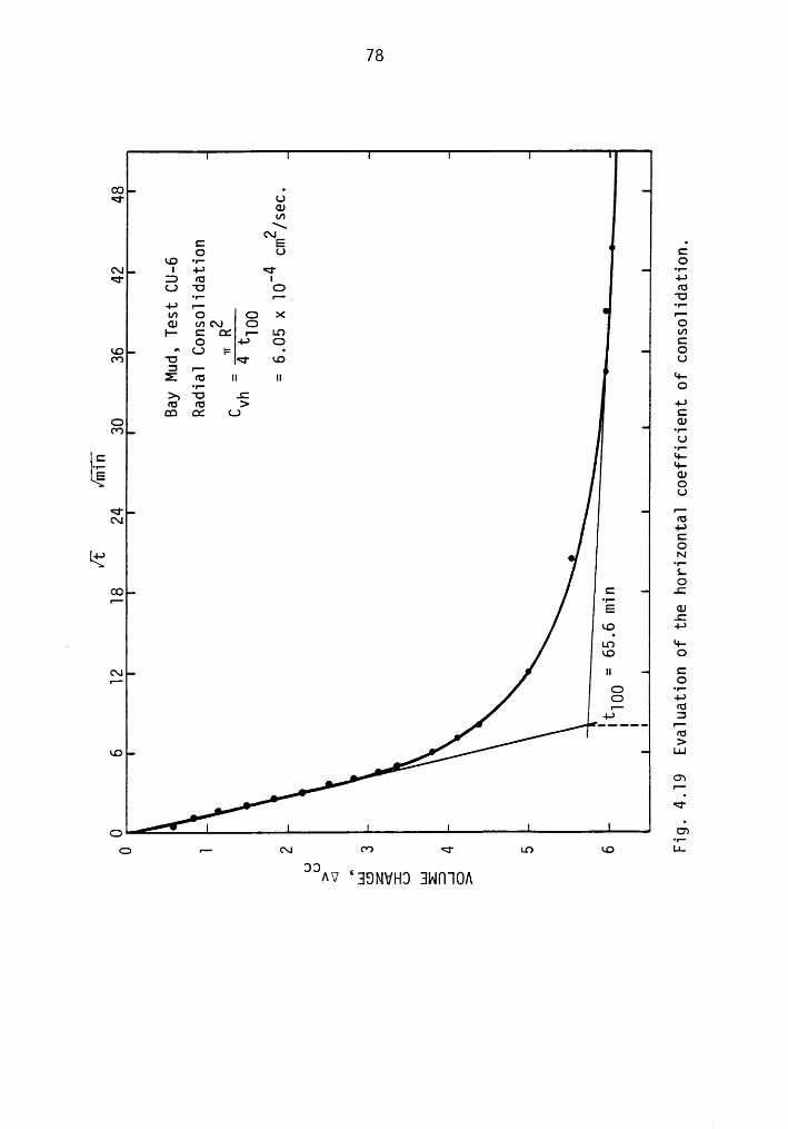
78

O<|' U

GJU)R(\I

C E •O U C

KO ·•— Q(\I I ·l-* <' •!—<r IJ cu u 4->

LJ 'U @ fü·n·· r-

‘¤4-* 1- •¤-U7 Ö Ü >< ITGJ U7f„\) G OF" C 1 r— LC7 U)

O 4-* G CKO ^ LJ L= · OO') 'U <' KO U

3 r-·Z eu n u <+-.,. O

>; ‘O .Cfü fü > +-*C.) C

CU(*7 •r-

U••-C

‘+-.,.. q.E (D

OU

Q' r-(\I fü

4-*COl;_—· ~••-S-O

® C .C•— •r—E GJ

.CKO 4-*

- LO 9-KO O

C\.| II C¤—· OCD ·•·C) 4-*n- IU

4-* 3iziitfü

>KO LLJ

O3r-<‘

® C7'I‘

r—· C\.I f*7 LO KO LI-

39 ‘^V EISNVHTJ HNITIO/\

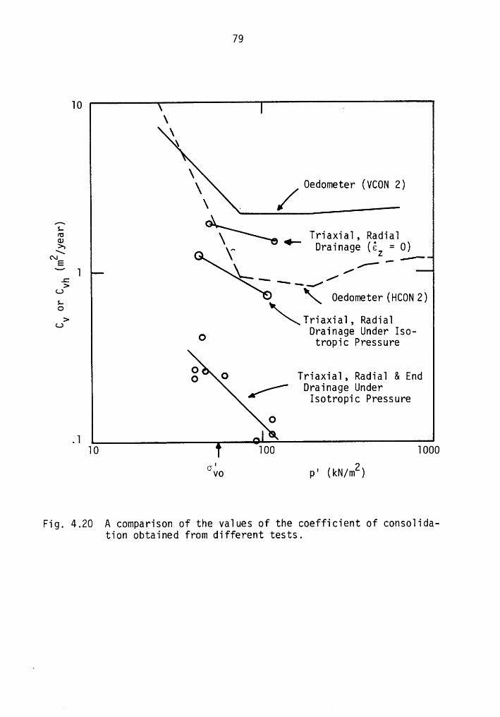
79

10 .\\\

\\ Oedometer (VCON 2)

T• • ~I R d' 'Iriaxia , a ia

ä\ ,.

‘—Drainage (é = 0)

g>>L‘\\_ 0edometer(HCON2)

oLj> ‘\\\\_Triaxial, Radial

O Drainage Under Iso-tropic Pressure

O . . .O 0 Triaxial, Radial & End

Drainage UnderIsotropic Pressure

O

.1 -10 100 1000G10 p' (kN/mz)

Fig. 4.20 A comparison of the values of the coefficient of consolida-tion obtained from different tests.

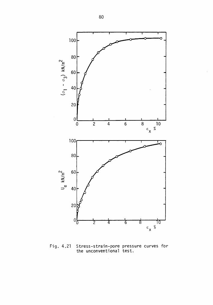
80

100

80cx:E\E 60 ·Amo°,_ 40

320

0 2 4 6 8 106X %100

80

\E=°’ 40

20

00 2 66 %X

Fig. 4.21 Stress-strain-pore pressure curves forthe unc0nventi0na1 test.

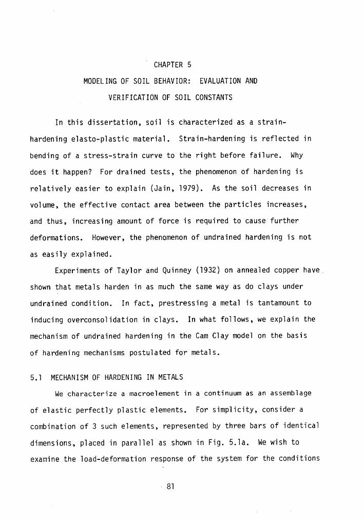
lCHAPTER 5

MODELING OF SOIL BEHAVIOR: EVALUATION AND

, VERIFICATION OF SOIL CONSTANTS

In this dissertation, soil is characterized as a strain-

hardening elasto—plastic material. Strain-hardening is reflected in

bending of a stress-strain curve to the right before failure. why

does it happen? For drained tests, the phenomenon of hardening is

relatively easier to explain (Jain, l979). As the soil decreases in

volume, the effective contact area between the particles increases,

and thus, increasing amount of force is required to cause further

deformations. However, the phenomenon of undrained hardening is not

as easily explained.

Experiments of Taylor and Quinney (l932) on annealed copper have.

shown that metals harden in as much the same way as do clays under

undrained condition. In fact, prestressing a metal is tantamount to

inducing overconsolidation in clays. In what follows, we explain the

mechanism of undrained hardening in the Cam Clay model on the basis

of hardening mechanisms postulated for metals.

5.l MECHANISM OF HARDENING IN METALS

we characterize a macroelement in a continuum as an assemblage

of elastic perfectly plastic elements. For simplicity, consider a

combination of 3 such elements, represented by three bars of identical

dimensions, placed in parallel as shown in Fig. 5.la. we wish to

examine the load-deformation response of the system for the conditions

— 8l

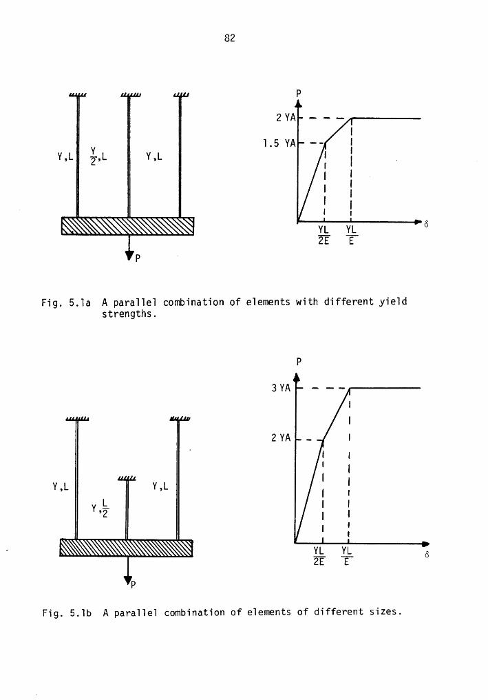
82

I I II I 2vA ---I I ¤I I.5 YA ··— I

v,L ät v,¤. I I _ _C II LI I I

% IL IE E

.

Fig. 5.la A parallel combination of elements with different yieldstrengths.

P

3YA -··— -II

ZYA - I

I Iv,L v,L I

L I II

'· I° II % IP

Fig. 5.lb A parallel combination of elements of different sizes.

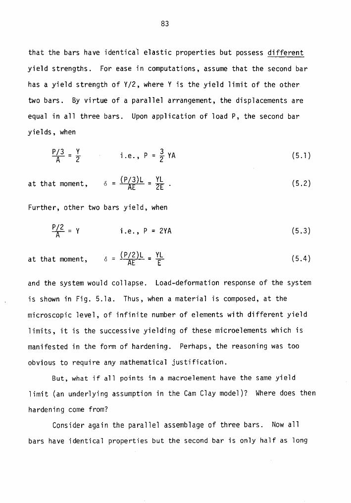
83

that the bars have identical elastic properties but possess different

yield strengths. For ease in computations, assume that the second bar

has a yield strength of Y/2, where Y is the yield limit of the other

two bars. By virtue of a parallel arrangement, the displacements are

equal in all three bars. Upon application of load P, the second bar

yields, when

$=§ 2 l.€.,P=§·YA (6.1)at that moment, 6 = igéélk-= ;% . (5.2)

Further, other two bars yield, when

?%= v 1.6., P = 2YA (6.2)

at that moment, 6 = iBlglk—= ik (5.4)AE E

and the system would collapse. Load-deformation response of the system

_ is shown in Fig. 5.la. Thus, when a material is composed, at the

microscopic level, of infinite number of elements with different yield

limits, it is the successive yielding of these microelements which is

manifested in the form of hardening. Perhaps, the reasoning was too

obvious to require any mathematical justification.

But, what if all points in a macroelement have the same yield _

limit (an underlying assumption in the Cam Clay model)? Where does then

hardening come from?

Consider again the parallel assemblage of three bars. Now all

bars have identical properties but the second bar is only half as long

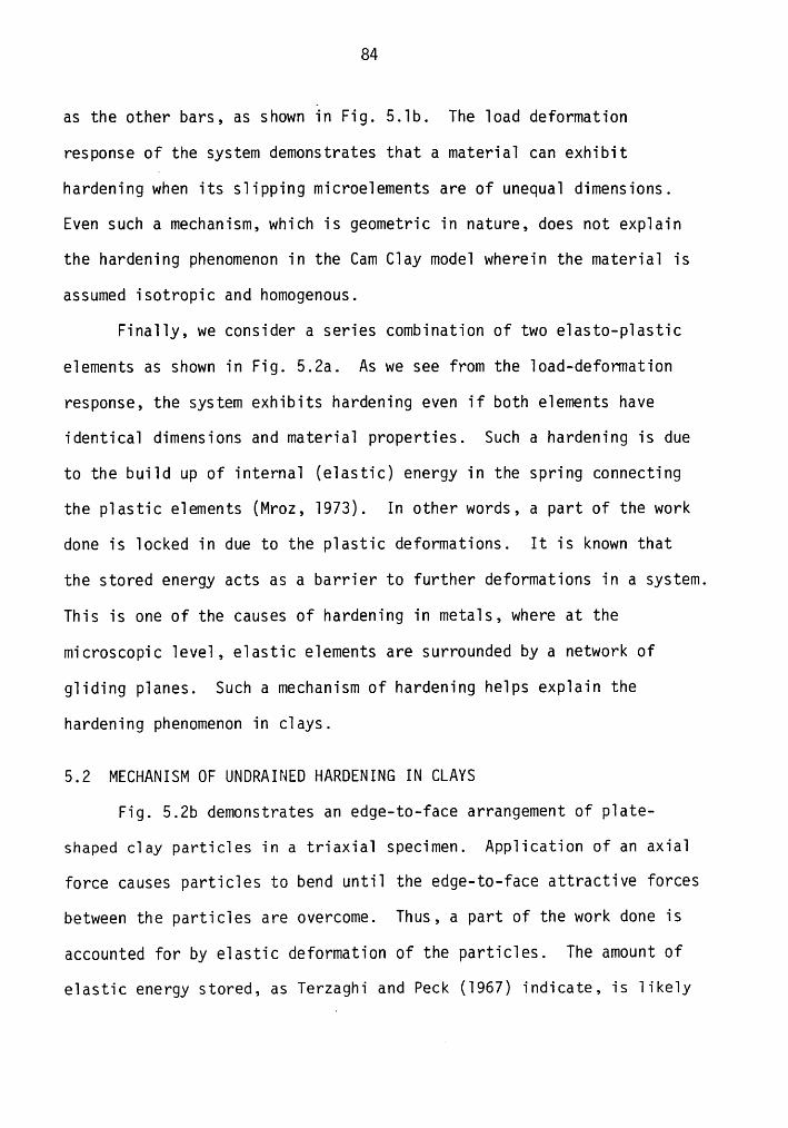
84

as the other bars, as shown in Fig. 5.lb. The load deformation

response of the system demonstrates that a material can exhibit

hardening when its slipping microelements are of unequal dimensions.

Even such a mechanism, which is geometric in nature, does not explain

the hardening phenomenon in the Cam Clay model wherein the material is

assumed isotropic and homogenous.

Finally, we consider a series combination of two elasto-plastic

elements as shown in Fig. 5.2a. As we see from the load-deformation

response, the system exhibits hardening even if both elements have

identical dimensions and material properties. Such a hardening is due

to the build up of internal (elastic) energy in the spring connecting

the plastic elements (Mroz, l973). In other words, a part of the work

done is locked in due to the plastic deformations. It is known that

the stored energy acts as a barrier to further deformations in a system.

This is one of the causes of hardening in metals, where at the

microscopic level, elastic elements are surrounded by a network of

gliding planes. Such a mechanism of hardening helps explain the

hardening phenomenon in clays.

5.2 MECHANISM OF UNDRAINED HARDENING IN CLAYS

Fig. 5.2b demonstrates an edge—to-face arrangement of plate-

shaped clay particles in a triaxial specimen. Application of an axial

force causes particles to bend until the edge—to-face attractive forces

between the particles are overcome. Thus, a part of the work done is

accounted for by elastic deformation of the particles. The amount of

elastic energy stored, as Terzaghi and Peck (l967) indicate, is likely

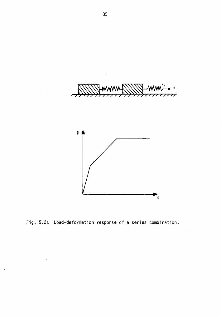
85

P

[

6

Fig. 5.2a Load-deformation response of a series combination.

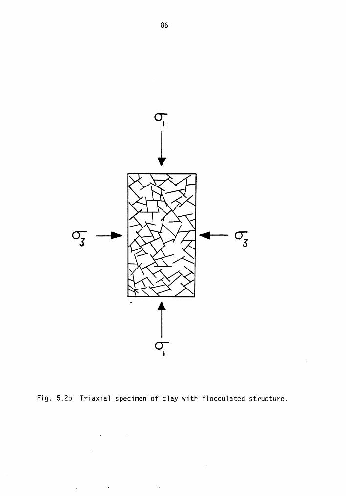
86

GT

n,gu 1‘ éxcg —» ‘,;§ { <—— cgäx

OT

Fig. 5.2b Triaxiai specimen of ciay with fiocculated structure.

87

to be different for different clay types. In a sand—mica mixture,

for example, much of the deformation is caused by elastic bending or

restitution of the grains. Also, with Fig. 5.2b, it becomes clear thatclays with flocculated structure will show a greater amount of un-drained hardening than the clays with dispersed structure.

A conclusion may be deduced from the foregoing discussion. It is

the unloading index, CS, which primarily governs the extent of un-

drained hardening in clays. 8

In soils, hardening may also be visualized as coming from the

build up of pore pressure due to shear. An increase in pore pressure

causes the mean effective stress in a specimen to decrease which en-

tails an elastic expansion of the soil skeleton. Since no change in

volume is permitted in an undrained test, an elastic expansion must be

compensated for by a plastic compression of equal magnitude. A plastic

compression causes yield surface to expand, which necessarily implies

a hardening phenomenon. Likewise, a decreasing pore pressure during

shear entails a contracting yield surface (if the theory at all per-

mits such a contraction) leading to the phenomenon of strain softening.

5.3 CAMBRIDGE SOIL MODELS

Calladine (l963) extended the classical work of Drucker, Gibson,

and Henkel (l957) to establish that normally consolidated clay was a

strain—hardening plastic material also in the undrained condition and

thus could be modelled within the realm of mathematical theory of

plasticity. In particular, Calladine showed how the concepts of

critical state soil mechanics, then advanced by Roscoe and co—workers

88

(1958,1963) cou1d be combined with the p1asticity theory to derive

stress-strain re1ations for soi1s. within a year of Ca11adine's work,

there came the first Cambridge soi1 mode1 (Roscoe and Schofie1d, 1963)

which was 1ater to be known as the Cam C1ay mode1 (Schofie1d and

wroth, 1968).

By drawing ana1ogy between the experiments of Tay1or and Quinney

(1932) on meta1 tubes under combined axia1 pu11 and torque with the

behavior of norma11y conso1idated c1ay in triaxia1 compression tests

Ca11adine postu1ated that the yie1d surface for the c1ay might be

e11iptica1. The suggestion was 1ater quantified by Roscoe and Bur1and

(1968) in what became 1ater the "modified Cam C1ay mode1." This is the

mode1 used in this dissertation. A brief account of the mode1, with

emphasis on undrained behavior, fo11ows.

Roscoe et a1. (1958) showed that for a norma11y conso1idated

saturated c1ay the void ratio e was a unique function of the mean norma1

stress p' and the deviator stress q. Based on experimenta1 data, they

were ab1e to show that a11 possib1e 1oading paths for a c1ay specimen

1ayed on a unique curved surface in the p',q,e space which they ca11ed

the "yie1d surface." The surface was 1ater renamed as the "state

boundary surface." A typica1 such surface for norma11y or 1ight1y over-

conso1idated c1ays is shown in Fig. 5.3.

Let us consider a triaxia1 specimen norma11y conso1idated to a

point E on the norma1 conso1idation 1ine PER in e-p' p1ane. Now, we

have two choices: Either to shear the specimen, in which case the

specimen wi11 fo11ow the path PS under undrained condition on the state

boundary surface; or, un1oad the specimen under isotropic pressure to

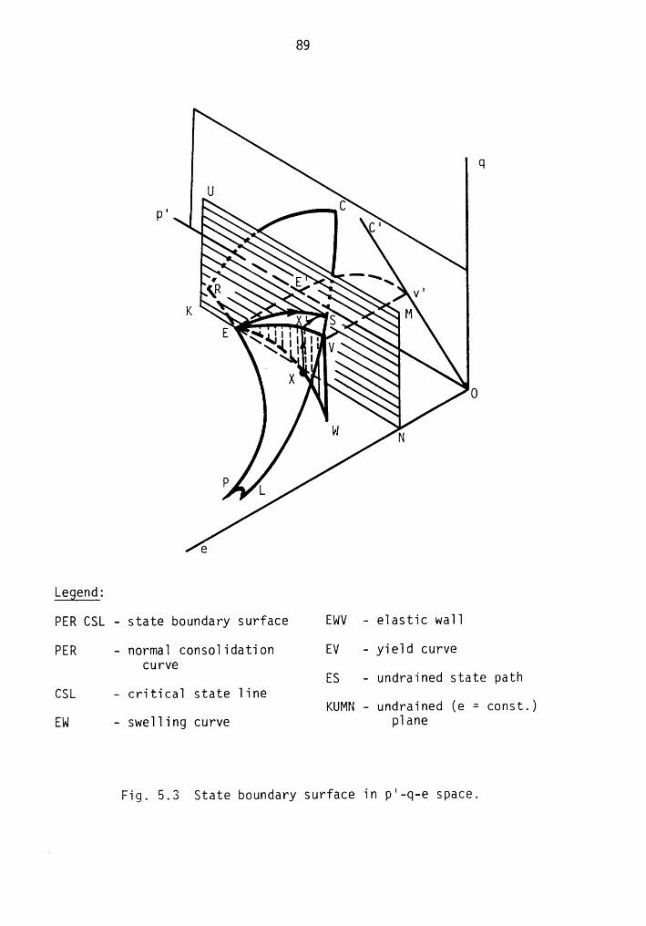
89

Q

P ‘« ~WW O

P NP L

e

Legend:PER CSL - state boundary surface EWV - elastic wall

PER - normal consolidation EV - yield curveCUY‘V€

ES - undrained state pathCSL — critical state line

KUMN — undrained (e = const.)Ew - swelling curve plane

Fig. 5.3 State boundary surface in p'-q—e space.

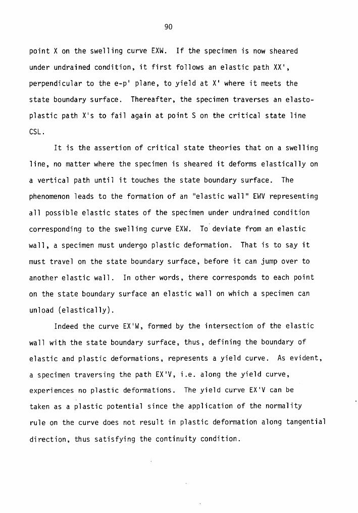
90

point X on the swelling curve EXW. If the specimen is now sheared

under undrained condition, it first follows an elastic path XX',

perpendicular to the e-p' plane, to yield at X' where it meets the

state boundary surface. Thereafter, the specimen traverses an elasto-

plastic path X's to fail again at point S on the critical state line

CSL.

It is the assertion of critical state theories that on a swelling

line, no matter where the specimen is sheared it deforms elastically on

a vertical path until it touches the state boundary surface. The

phenomenon leads to the formation of an "elastic wall" EWV representing

all possible elastic states of the specimen under undrained condition

corresponding to the swelling curve EXW. To deviate from an elastic

wall, a specimen must undergo plastic deformation. That is to say it

must travel on the state boundary surface, before it can jump over to

another elastic wall. In other words, there corresponds to each point

on the state boundary surface an elastic wall on which a specimen can

unload (elastically).

Indeed the curve EX'w, formed by the intersection of the elastic

wall with the state boundary surface, thus, defining the boundary of

elastic and plastic deformations, represents a yield curve. As evident,

a specimen traversing the path EX'V, i.e. along the yield curve,

experiences no plastic deformations. The yield curve EX'V can beA

taken as a plastic potential since the application of the normality.

rule on the curve does not result in plastic deformation along tangential

direction, thus satisfying the continuity condition.

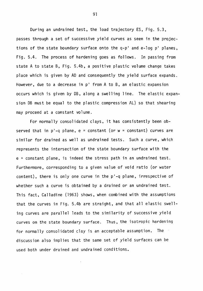
9l

During an undrained test, the load trajectory ES, Fig. 5.3,

passes through a set of successive yield curves as seen in the projec-

tions of the state boundary surface onto the q-p' and e—log p' planes,

Fig. 5.4. The process of hardening goes as follows. In passing from

state A to state B, Fig. 5.4b, a positive plastic volume change takes

place which is given by AD and consequently the yield surface expands.

However, due to a decrease in p' from A to B, an elastic expansion

occurs which is given by DB, along a swelling line. The elastic expan-

sion DB must be equal to the plastic compression AL) so that shearing

may proceed at a constant volume.

For normally consolidated clays, it has consistently been ob-

served that in p'-q plane, e = constant (or w = constant) curves are

similar for drained as well as undrained tests. Such a curve, which

represents the intersection of the state boundary surface with the

e = constant plane, is indeed the stress path in an undrained test.

Furthermore, corresponding to a given value of void ratio (or water

content), there is only one curve in the p'-q plane, irrespective of

whether such a curve is obtained by a drained or an undrained test.

This fact, Calladine (l963) shows, when combined with the assumptions

that the curves in Fig. 5.4b are straight, and that all elastic swell-

ing curves are parallel leads to the similarity of successive yield

curves on the state boundary surface. Thus, the isotropic hardening

for normally consolidated clay is an acceptable assumption. The

discussion also implies that the same set of yield surfaces can be

used both under drained and undrained conditions.

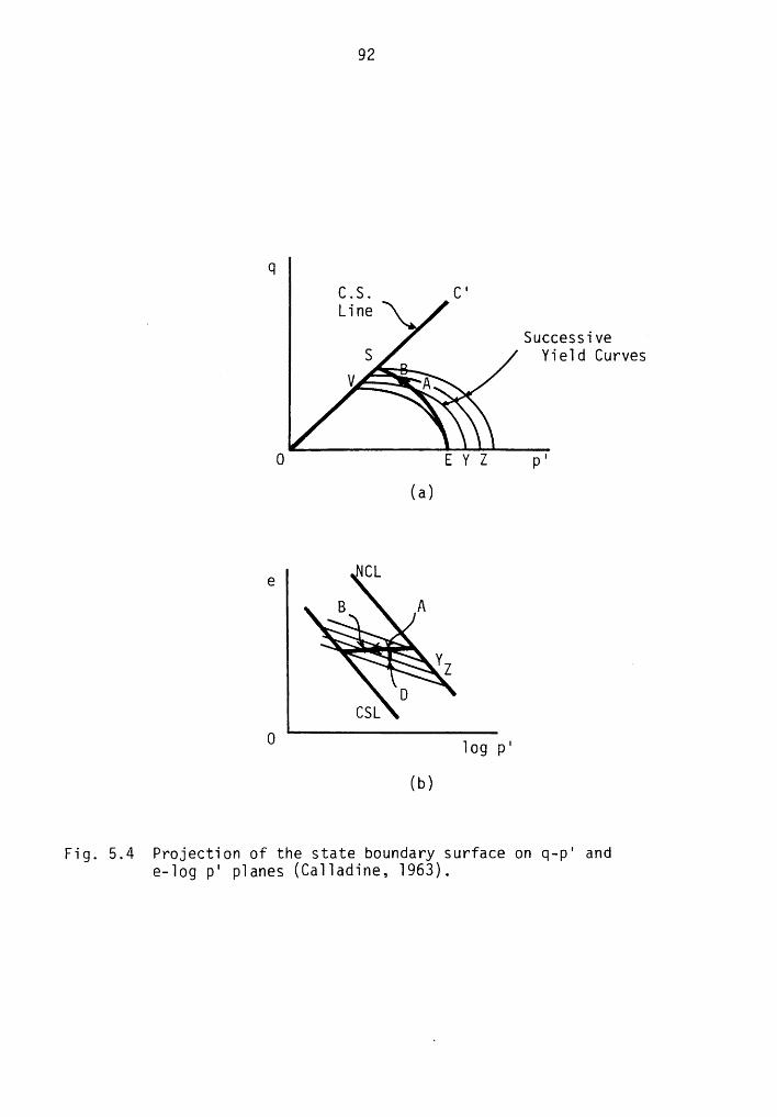
92

9C.S. C'Line

SuccessiveS _ Yie1d CurvesVi

0 E Y Z p'(a)

E NCLB A

Yz

DCSL

0 I10g p(b)

Fig. 5.4 Projection of the state boundary surface on q—p' ande—10g p' p1anes (Ca11adine, 1963).

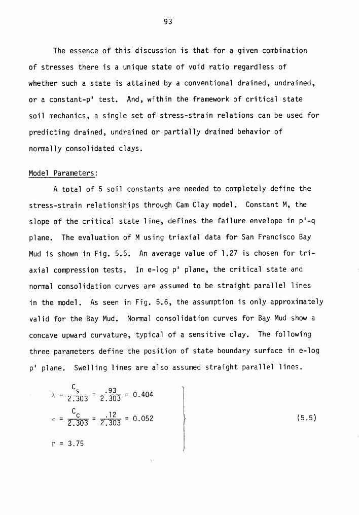
93

The essence of this discussion is that for a given combination

of stresses there is a unique state of void ratio regardless of

whether such a state is attained by a conventional drained, undrained,

or a constant-p' test. And, within the framework of critical state

soil mechanics, a single set of stress-strain relations can be used for

predicting drained, undrained or partially drained behavior of

normally consolidated clays.

Model Parameters:

A total of 5 soil constants are needed to completely define the

stress-strain relationships through Cam Clay model. Constant M, the

slope of the critical state line, defines the failure envelope in p'—q

plane. The evaluation of M using triaxial data for San Francisco Bay

Mud is shown in Fig. 5.5. An average value of l.27 is chosen for tri-

axial compression tests. In e-log p' plane, the critical state and —

normal consolidation curves are assumed to be straight parallel lines

in the model. As seen in Fig. 5.6, the assumption is only approximately

valid for the Bay Mud. Normal consolidation curves for Bay Mud show a

concave upward curvature, typical of a sensitive clay. The following

three parameters define the position of state boundary surface in e-log

p' plane. Swelling lines are also assumed straight parallel lines.

C

K 0.062 (6.6)V = 3.75

C

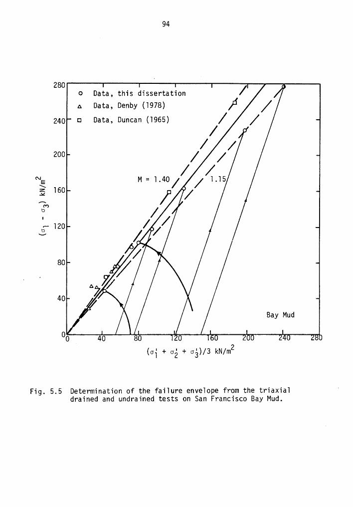
94

280 ( 1 ,G Data, this dissertation /A Data, Denby (1978) jf /

240 ¤ Data, Duncan (1965) / /

200 / /“‘ M = 1.40

///1015E160’F¤

T /·— 120 /

380 __

. A7?40 /’/ Bay Mud

0 O0 40 80 0 •• •• ¤• .•(oi + oé + oé)/3 kN/m2

Fig. 5.5 Determination of the fai1ure enve1ope from the triaxia1 ‘drained and undrained tests on San Francisco Bay Mud.

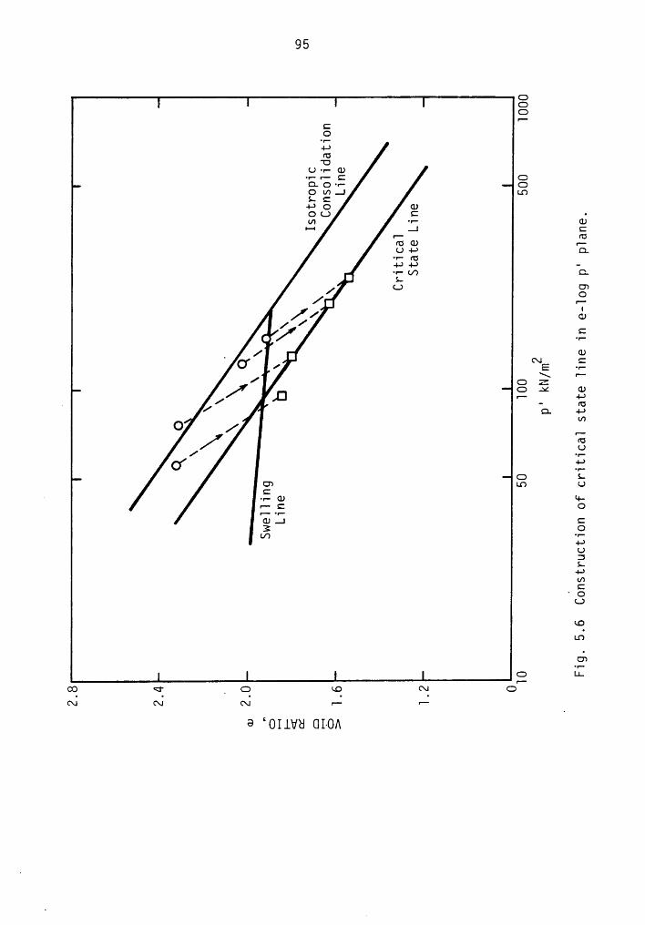
95

GGGfi

O'!*+-3(U'O

U·r—·CD·r··r—-EOm.!

LOLC4-*O CUOC.) C •m •r— GJ*-" .1 C•— FUSB 5•r¤•(¤

+-3+-* -••—l/) O.L

/ L.) U3/ E|/F/ cu/// .s

_ / CDO' , NE E/ c:» FF

/ D 0Ad./ " - E/ :1 -•->

mO /(U/ Fcf fi

G LCD LO UC' •r·GJ '~+—r—C Of'*'|*%—' 5"’ I3

U3fs(J)C‘O

L.)

LOLO

6-'F"G L!.

FQ

OO Q _ G LO <\! GC\I C\| C\! r--

•*

3 ‘011va uLOA

96

where P, the critical void ratio at unit pressure, is read from Fig.

5.6. .Finally, the elastic shear modulus G is introduced into the

model through the ratio G/SU. Taking an average of four undrained

tests, Table 4.5, G/SU = 250 is adopted in this work. Expressions for

undrained strength SU are derived in the following section.

Undrained Strength in Cam Clay:

Failure occurs when the loading path meets the critical state

line, whereupon shear stress takes on a value,

qf = M p} (5.6)

i.e.,s—'M· (67)u ” 2” pf °

But p} can be computed from the equation of the critical state line in

e-log p' plane, since the void ratio eo remains unchanged during un-

drained deformations; i.e.

eo = P - A tn pé (5.8)

or p% = exp [(P - eo)/A] (5.9)

Therefore,

SU = %—M exp [(P - eo)/A] (5.10)

Eq. (5.l0) can be expressed as,

w + gl tn S = constant (5.ll)S uAnd thus, the Cam Clay model envisions a straight line relationship be-

tween the water content w and the log of shear strength. Now, it also

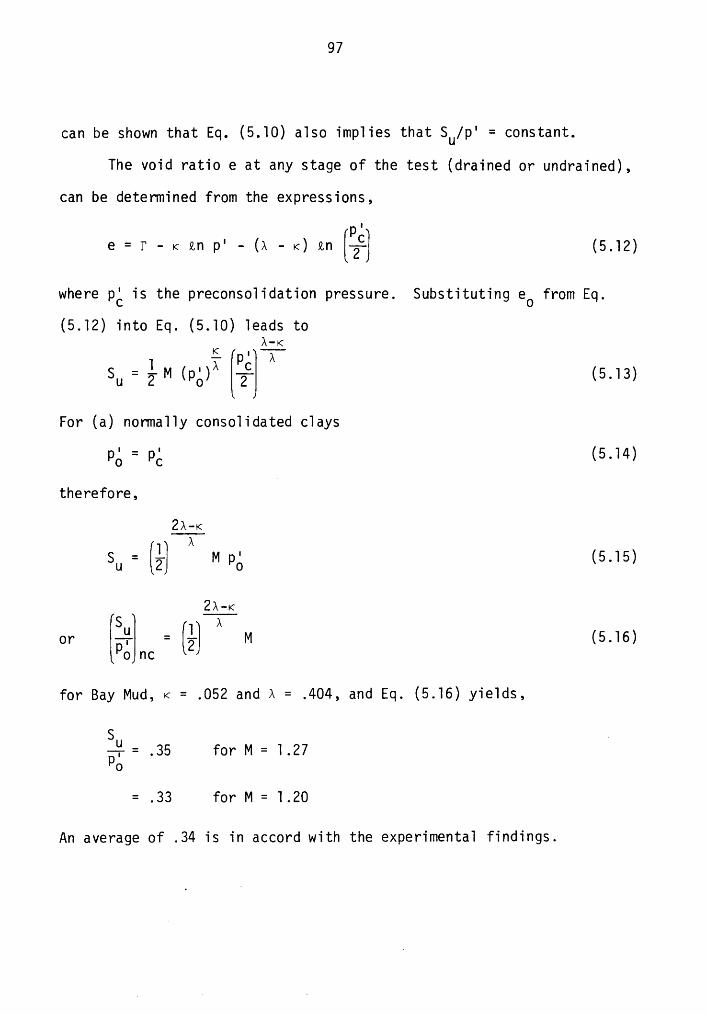
97

can be shown that Eq. (5.10) a1so imp1ies that SU/p' = constant.

The void ratio e at any stage of the test (drained or undrained),

can be determined from the expressions,pl

e = P - K tn p' - (A — K) tn (5.12)

where pé is the preconso1idation pressure. Substituting eo from Eq.

(5.12) into Eq. (5.10) 1eads toK 2:5.. p' Ä

Su (5.13)

For (a) norma11y conso1idated c1ayspé = pg (5.14)

therefore,ZA-K

1 ASU Z (ä] M pg (6.16)

2Ä-KS AOK .9 Z M (5.16)po nc

for Bay Mud, K = .052 and A = .404, and Eq. (5.16) yie1ds,

SU 1—T = .35 for M = 1.27po

= .33 for M = 1.20

An average of .34 is in accord with the experimenta1 findings.

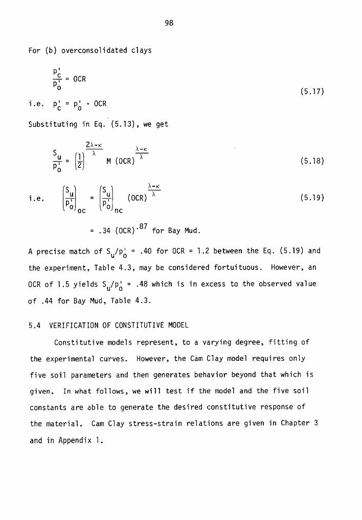
98

For (b) overconso1idated c1ays

pl—$-= OCRpo

(5.17)i.e. pé = pg · OCR

Substituting in Eq. (5.13), we get

2A-K _Su V]-? ¥7 = — M (0612) 5.18po 2 2 ( )5 S Äii.e. [B?} = [E2} (OCR) Ä (5.19)

O oc O nc

= ,34 (0CR)°87 for Bay Mud.

A PY‘€C1$€ match of = -4O fOY‘ OCR = 1.2 between the Eq. (5.19) and

the experiment, Tab1e 4.3, may be considered fortuituous. However, an

OCR of 1.5 yie1ds SU/pé = .48 which is in excess to the observed va1ue

of .44 for Bay Mud, Tab1e 4.3.

5.4 VERIFICATION OF CONSTITUTIVE MODELConstitutive mode1s represent, to a varying degree, fitting of

the experimenta1 curves. However, the Cam C1ay mode1 requires on1y

five soi1 parameters and then generates behavior beyond that which is

given. In what fo11ows, we wi11 test if the mode1 and the five soi1

constants are ab1e to generate the desired constitutive response of

the materia1. Cam C1ay stress-strain re1ations are given in Chapter 3

and in Appendix 1.

99

(a) Undrained Tests:-

Stress-strain-pore pressure curves under triaxial conditions were

computed for Bay Mud under consolidation pressures equal to those of

tests CU-2 and CU-3. Predicted and experimental curves are shown in

Figs. 5.7 and 5.8. The model shows a slightly stiffer response.

That the Modified Cam Clay model provides predictions of too

stiff a behavior in undrained shear has been a general observation pre-

viously. The problem is in part attributed to the assumed elliptical

shape of the yield surface, which does not produce enough shear strains

at the low values of shear stress. Alternatives lie in either formu-

lating a composite surface of different arc types or resorting to the

original bullet-shaped Cam Clay surface. Both of these proposals were

investigated and it was found that even though an improved undrained

response could be obtained, the modifications created additional limita-

tions. Thus, the slight error in response that exists with the

elliptical surface has been accepted.

A crucial aspect of the undrained modeling is the generation of

excess pore pressures due to shear. In light of the previous discus-

sion, a question can be raised: "Is there a mechanism in the Cam Clay

model which generates pore pressures due to shear? If so, is it

adequate?" Fortunately the model gives reasonable prediction of pore

pressures for both CU tests, as seen in Figs. 5.7 and 5.8, providing

evidence of the model's capability to represent the phenomenon well.

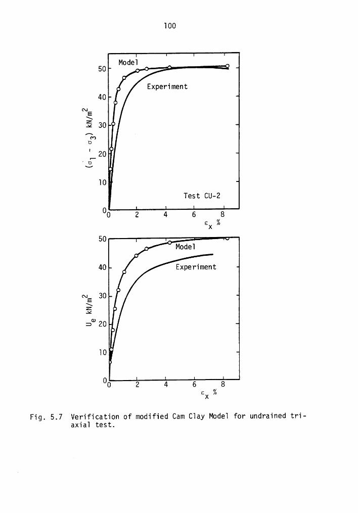
100

Mode150 •

'• _—•

, Experiment40 _

C\lE\E 30 •

¤'_ 20 °QB I

10,

Test CU-2 A00 2 4 6 8ex %

50 _ -1 ·• MOd€·|

40 _ Experiment

NE 30I: O¤°’ 20,

10 1*

00 2 4 6 6Ex

Fig. 5.7 Verification of modified Cam C1ay Mode1 for undrained tri-axia1 test.

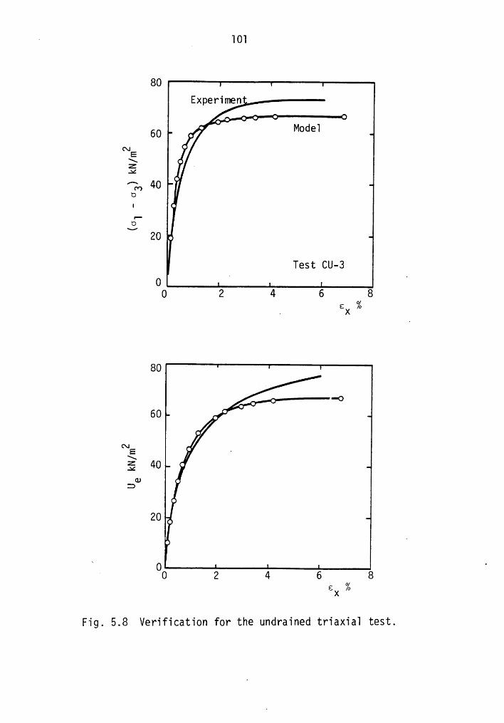
4 6 101

00Experimen

60 _ · °° Modelc\| O

E\ •

^ 40 °6* II O

20 60Test CU—3

0 2 4 6 00 ex %

00

60 ,· °

..6 /\ /fc 40 •

CU •Z)

202 0 2 4 6 0

c %X

Fig. 5.8 Verification for the undrained triaxial test.

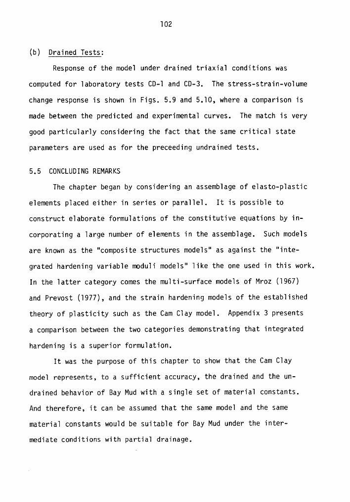
102

(b) Drained Tests:

Response of the mode1 under drained triaxia1 conditions was

computed for 1aboratory tests CD-1 and CD-3. The stress-strain-vo1ume

change response is shown in Figs. 5.9 and 5.10, where a comparison is

made between the predicted and experimenta1 curves. The match is very

good particu1ar1y considering the fact that the same critica1 state

parameters are used as for the preceeding undrained tests.

5.5 CONCLUDING REMARKS

The chapter began by considering an assemb1age of e1asto-p1astic

e1ements p1aced either in series or para11e1. It is possib1e to

construct e1aborate formu1ations of the constitutive equations by in-

corporating a 1arge number of e1ements in the assemb1age. Such mode1s

are known as the "composite structures mode1s" as against the "inte-

grated hardening variab1e modu1i mode1s" 1ike the one used in this work.

In the 1atter category comes the mu1ti-surface mode1s of Mroz (1967)

and Prevost (1977), and the strain hardening mode1s of the estab1ished

theory of p1asticity such as the Cam C1ay mode1. Appendix 3 presents

a comparison between the two categories demonstrating that integrated

hardening is a superior formu1ation.

It was the purpose of this chapter to show that the Cam C1ay

mode1 represents, to a sufficient accuracy, the drained and the un-

drained behavior of Bay Mud with a sing1e set of materia1 constants.

And therefore, it can be assumed that the same mode1 and the same

materia1 constants wou1d be suitab1e for Bay Mud under the inter-

mediate conditions with partiai drainage.

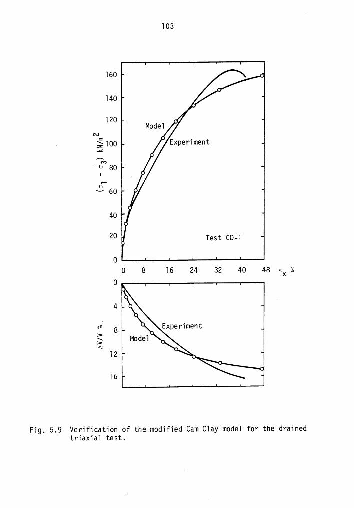
103

160 •

140

120 ,mE •

. ;;10O Experiment34’?6* 9 80

I IUf"

O

40

20 L Test co-10

0 8 16 24 32 40 48 ex %0

4 •

g 8 ••>Q OQ I12 ,

16

Fig. 5.9 Verification of the modified Cam C1ay mode1 for the drainedtriaxia1 test.

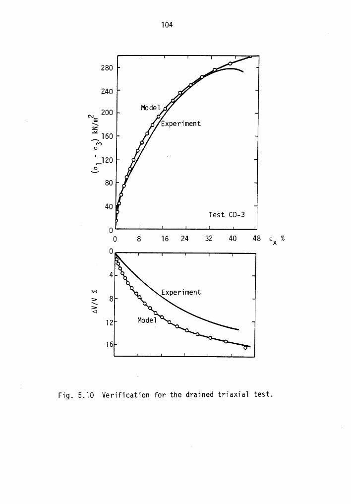
104

280 _, °O//•

240 ./•/

NE 200 _‘

E5. Experiment

„_160 °(Y) I

O O

'_120 ·‘

O •$.4 •’ I80 ,

E 40 _'I Test CD-3

00 8 16 24 32 40 48 ex %

0

463°• Experiment

> 8 °\ •> •< O

12 Mode1 ° .16 ° • _

Fig. 5.10 Verification for the drained triaxia1 test.

UCHAPTER 6

MODELING OF FIELD PRESSUREMETER TESTS:

AXISYMMETRIC-PLANE STRAIN ANALYSIS

The first step in the finite element simulation work was directed

towards establishing that the modeling procedures could reasonably

duplicate the observed field behavior in a pressuremeter test. For

this purpose, finite element analyses were performed for conditions

modeling those of ll of the pressuremeter tests of Denby (l978) and

Benoit (l983) in San Francisco Bay Mud. The tests cover a range of

depths from l6.4 to 49.l ft. (5 to l5 m) and allow a thorough test of

the modeling procedures (see Table 6.l).

A basic assumption of all pressuremeter theories is that the soil

surrounding the probe deforms following the condition of axial sym-

metry and plane strain. Using this assumption the expense of conduct-

ing a finite element analysis can be greatly reduced by modifying an

axisymmetric FE formulation for the additional condition of plane

strain. In such a case, ez = O, and therefore, the stress-strain rela-tion reduces to the form

6; EPl{62 = [pgp]

{ 0 (6.l)0, 3x3 é(00

The finite element formulation is obtained by integrating a one-

dimensional element axisymmetrically around the cavity-—in the hori-A

zontal plane. In this work,-a total of 76 two noded elements, L2P2,

lO5

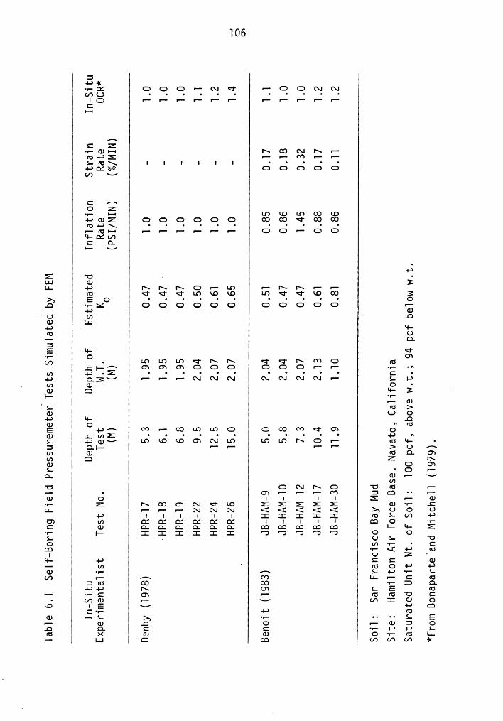
34-*·4<•-I O O O FZ (\l Ü I- O O (\] Gl(AU • • • • • • • • • • •

I Q I- I-- I- r- IZ IZ IZ I- I- YZ IZC

•--·I

L-C Z·I— G)!-I Ä O C\I Ä I-fü·4—*Z Pi FZ O IZ I-L I'¤\ I I I I I I • • • • •4-*QCä O O O O Ogf) O

C z·sO Z·I- •—• LD LO LO O LD4-* GJX O O O O O O O O Ü O O;¤.p\ I I I I I I I I I I IIi fü!-• I- IZ I- IZ IZ fi O O I" O O*4-ZV)C QI—• O

4-*E 'U - ·LIJ G) 3LI. 4-* Ä Ä Ä O IZ LO I- Ä Ä IZ IZ

fü Ü Ü Ü LO LO LO LO Ü Ü LO O 3Ä E O • • • • • • • • • • n O

” 'O U) .OGJ l.I.I4-* *4-fü UIZ Q

3E *4- Ü·I— Q C7I;) I LO LO LO Ü I\>|\ Ü Ü Ä (*7 O I5

Ch ON OW O G G O O O I- I'- ·I— ·•'~U) 4-) gz I I I I I I I I I I I g4,.) Q3- I- FZ IZ C\I C\l C\I (\| (\| Gi GI I" L -I-*

. In GJ O · _GJ Q *4- 3I- ·I-‘ IZ GJL fü >GJ O O4-* *4·- .QGJ O " füE J.)- 0*7 I- OO LO LO G O OO (*7 Ü 07 QG, I I I I I I I I I I I I 4) 6L .I.> gp- LO LO LO O7 <\I LO LO LO N G IZ I5 II- I3 Q_}.- r'- I- I'- IZ > Q) rsIn GJ ru Q. G7In Q Z NGJ O C7L ^ IZQ__ Q) I- x./

U1-O O (\] Ä O -O fü IZI- • C7 IZ IZ IZ O 3 O " I"GJ 0 I I I I I Z IZ GJ·I- z I\ oo ow cx: <I· nc E Z Z Z Z GJ ·I— .:LL IZ I- I- mn cu cu < <E < < < >I LJ 0 0

4-* I I I I I I I I I I I fü X (./7 4-*Cn In M M M M M M I I I I I cn 0 ·I-C GJ Q Q Q Q Q Q CQ CQ O CQ LI- *4- E'I* I- I I I I I I 'O 'O O 'D 'O O OL ~ U L 'OO UT ·I- • E

CO ·I— <[ +-* füI LJ 3 '

*4- 4-* C C GJIZ I/7 ' fü O 4-* 4-*G) ·I— r'- L 4-* ·I— L(/) IZ LI. IZ C fü

3 fü O O ·I— O Q.-I->-I-I Ix ow s: E co

I- ·I— C C7 I"" fü fü C· L/7 GJ I- -/ L/7 I GJ O

LD I E -/ 4-* QQCu- 4-* fü

Q) IC; L ä•'— •• •• L E

I" GJ .O O IZ CD 3 O.O O. C C •I— 4-* -4-* Lfü X GJ GJ O 'I" fü LI-I—- I.I.1 ca co In cn m —I<

107

with a disp1acement and a pore pressure degree of freedom at each node

are used to mode1 the 11 fie1d pressuremeter tests. The boundary

conditions assumed in the ana1yses are shown in Fig. 6.1.

6.1 MODEL PARAMETERS

On1y two additiona1 constants are required when an e1asto-p1astic

formu1ation is extended to inc1ude the pore-pressure degree of freedom;

the permeabi1ity of soi1 and the unit weight of water. Permeabi1ities

in horizonta1 and vertica1 directions, kh and kv, were determined fromthe resu1ts of oedometer and fie1d pressuremeter tests. Indeed, it is

a difficu1t task to ascertain the horizonta1 permeabi1ity of a stratum.

Benoit (1983) reports permeabi1ity va1ues of 3.5x1O”7 to 7x1O”7 cm/sec

for Bay Mud from his pressuremeter ho1ding tests. Comparing these

va1ues with the Taboratory determined horizonta1 permeabi1ity of

7x1O”8 cm/sec, it was decided to assign a va1ue of 3.5x1O”7 cm/sec to

horizonta1 permeabi1ity of Bay Mud under1ying the Hami1ton Air Force

Base Station.

The soi1 parameters emp1oyed in the finite e1ement simu1ation of

the pressuremeter tests are given in Tab1e 6.2. The Cam C1ay

parameters are the same as those used in the mode1ing of triaxia1 tests

ear1ier, excepting for the va1ue of M which is taken here at 1.2,

instead of 1.27 used for the triaxia1 tests. The va1ue of M for the

ana1yses was backfigured from the fie1d tests by finite e1ement mode1ing.

A va1ue of 1.2 provided the best fit for the se1f-boring pressuremeter

tests in Bay Mud whi1e keeping the other soi1 parameters una1tered.

The reason for the discrepancy in M va1ues wou1d appear to be re1ated

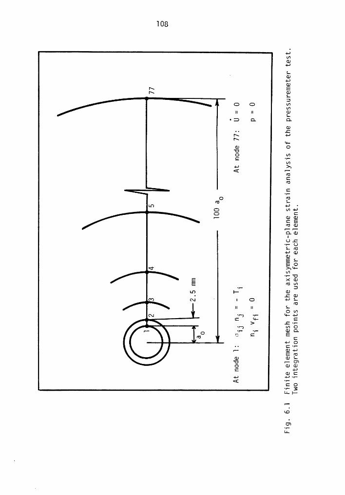
4-*L/7GJ

4-*LI GJ

4-*GJIx EN GJ

L” 3O O an

UIII II GJ

L-3 Q Q

CU•. _;N 4-*N LI-GJ O'OO mC •r—

V74-* >s{ r-

TUCTUC•r-

. O TUaj L

LO 4-* ·CD m~I—>O CIi GJGJ:E

TUGJQ.€UI(.J.C•'—U

LTU+-*0)GJELEO

<'U7E ><C1JE TUU')

·r- 3LO I- (U

· .CGJTO (\| ' I O «I—*L

TUII Il L

OU)(\| W7 •r— LI-4-*

C '·4— CL > c--·•·7 L/IOG 'r· •v—O C E·I—*O•• Cu-

1- Q)·I—*Ea:

GJ GJLO GJGJC 4-*CDC

-4-* -I—*·r—··<E ‘·—

CO.,...3LI-}-

FC

LO

O7'I"LI.

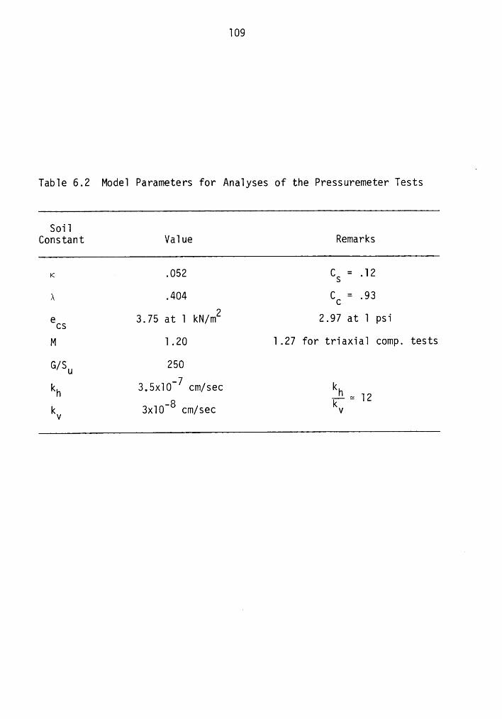
l09

Table 6.2 Model Parameters for Analyses of the Pressuremeter Tests

SoilConstant Value Remarks

l< — .052 CS = .—I2A .404 CC = .93ecs 3.75 at l kN/m2 2.97 at l psi

M l.20 l.27 for triaxial comp. tests

G/Sv 250k 3.5xl0-7 cm/sec kh .D.„ 12kv 3xl0"8 cm/sec kv

llO

to the effect of mode of failure. In the pressuremeter test, the

failure takes place in a vertical plane, as seen in Fig. 2.3 (Chapter

2), and neither a triaxial compression test nor an extension test can

simulate such a pattern of failure.

6.2 COMPARISONS: FIELD VS. MODEL

Figs. 6.2 to 6.lO give comparisons of the analytical pressure-

meter curves with the field curves. Generally speaking the model pre-

dicts the pressuremeter curves very well. This is encouraging in view

of the fact that only one set of soil parameters is used. It also

should be recognized that the analyses suggest that some drainage

occurs in the tests, a subject which will be discussed later.

A comparison of stress paths followed by an element of soil at

the cavity interface is shown in Figs. 6.ll and 6.l2. while the model

is able to generate the basic trend of the total stress path a dif-

ference is noted in the comparisons of effective stress paths. For

instance, consider test HPR-l9, Fig. 6.lla, the effective stress path

predicted by the model compares well with that of the field until point

F, i.e., in the prefailure stage. But, in the postfailure stage, the

predicted path stays at point F while that of field continues right-

ward. No satisfactory explanation could thus far be found for the

discrepancy observed.Fig. 6.l3 demonstrates one of the most significant observations

of the analysis. It shows the variation of vertical stress in a soil

element at the cavity interface as the test proceeds. Contrary to what

would be expected from the theory of elasticity, the effective vertical

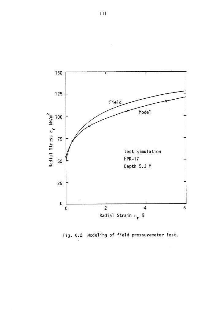
111

150

125

NE ' Mode1100o§ 75 „S.ä__ / Test Simu1ationrc ..3; 50 ' HPR—17

¤¤ Depth 5.3 M

25

‘0 2 4 6

Radia1 Strain er %

Fig. 6.2 Mode1ing of fie1d pressuremeter test.

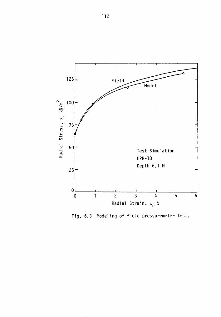
112

125 _ M0de1

***; 100 .$ .Z..>¢. /0 -.„;‘ 75$L •

-1->an

E 60-g Test Simu1ati0n“ HPR-18Depth 6.1 M

25

00 1 2 3 4 5 6

Radia1 Strain, er %

Fig. 6.3 M0de1ing of fie1d pressuremeter test.

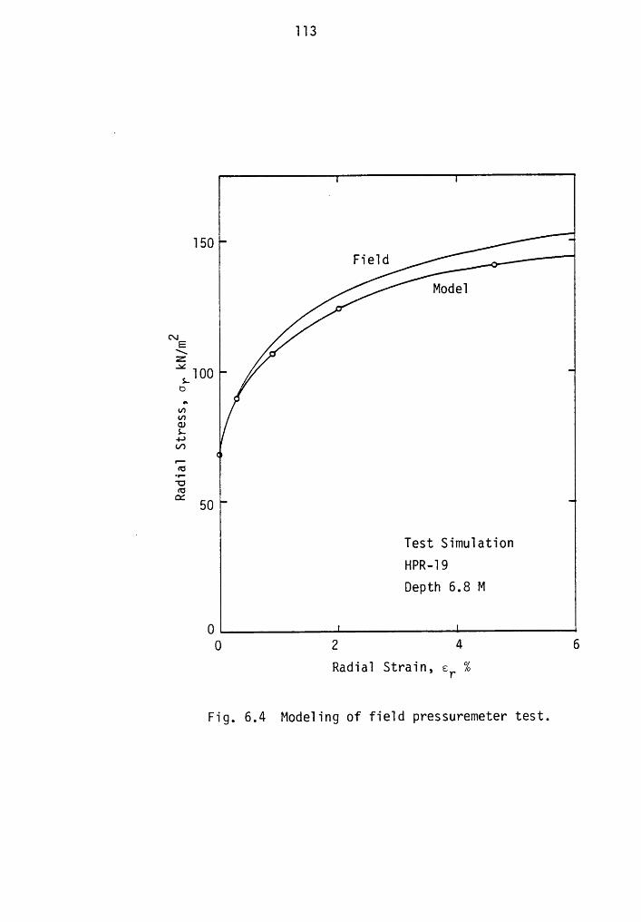
113

150

Model

C\|E\ .EL1006.529s.4->m

F6E&’

50l

Test SimulationHPR-19Depth 6.8 M

00 2 4 6

Radial Strain, er %

Fig. 6.4 Modeling of field pressuremeter test.

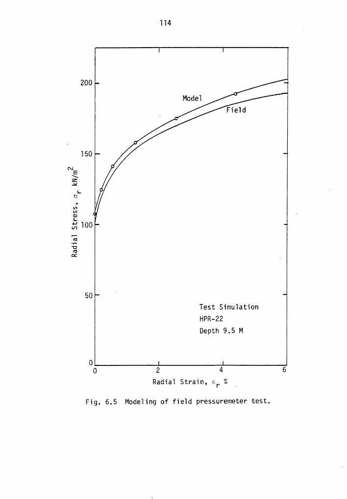
114

200

Fie1d

150

Exz:.4oJU)0.: ';—5,,100

F?Ero°‘ 0

50 ’

Test Simu1ati0nHPR-22Depth 9.5 M

Q .0 2 4 6

Radia1 Strain, Er%Fig.

6.5 Mode1ing of fie1d pressuremeter test.

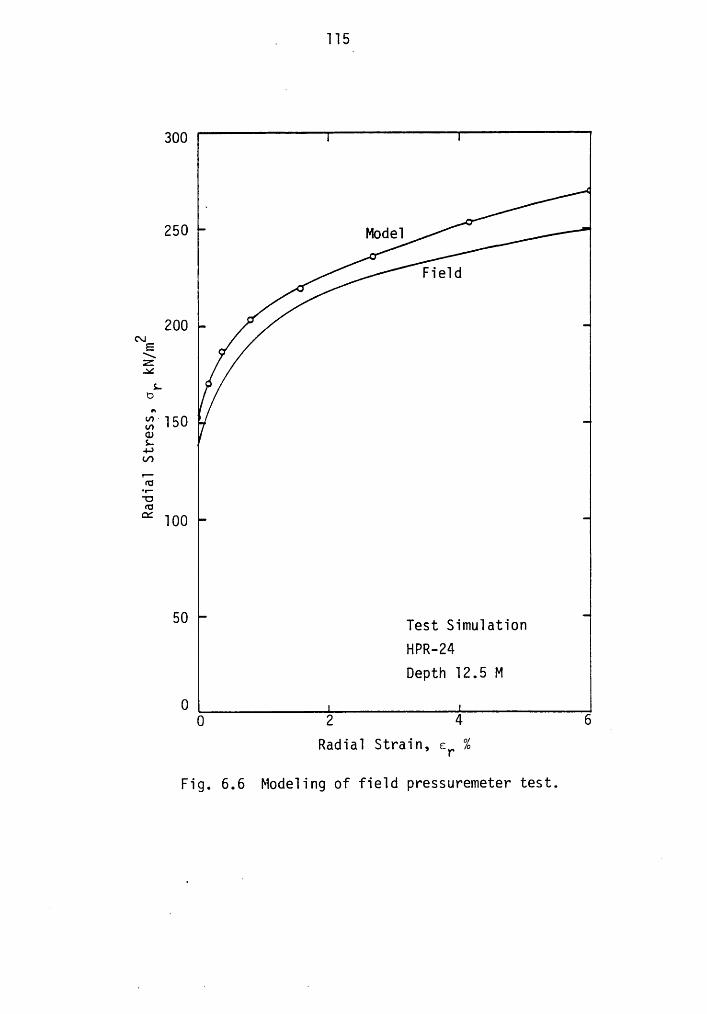
. 115

300

250 °

Fie1d

200 °cwE .xz.

ro

$:150 V<us.4->an

FEcc°‘ 100

50 iest s1m01at10nHPR-24Depth 12.5 M

00 2 4 6 _

Radia1 Strain, er %


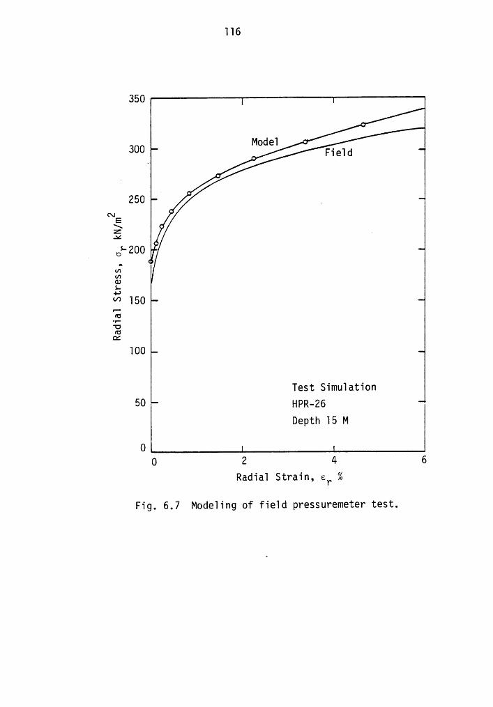
116

350

000 _ Fie1d

250• _

E\ •Z .x

V O*200 VanCDL.-s->“° 150F6-5cu .

100

Test Simu1ation50 HPR-26Depth 15 M

00 2 4 6

Radia1 Strain, er %

Fig. 6.7 Mode1ing of fie1d pressuremeter test.

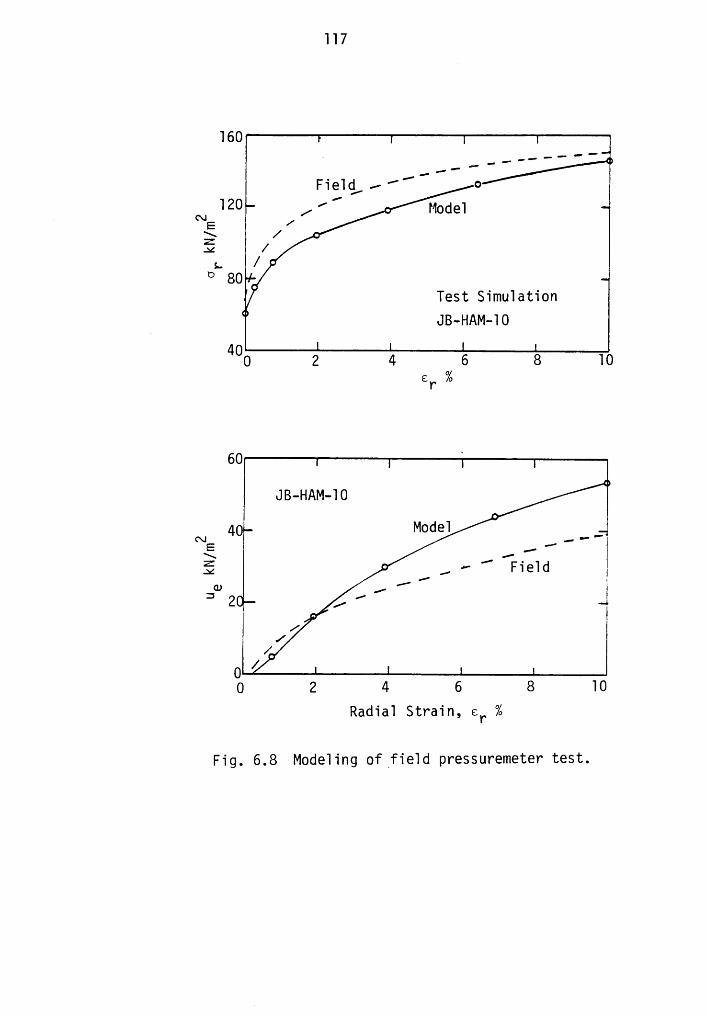
117

160

4 N 120/

> / •Z /

s.. / °° 80 _

Test Simu1ati0nU JB—HAM-10

400 2 4 6 8 10eY_%

60 ‘

JB-HAM-10

N AQMode1EE

_, ~ F1e1dcu ,

"° 2 ,/ .1//

/0 /0 2 4 6 8 10

Radia1 Strain, er %

Fig. 6.8 M0de1ing of_fie1d pressuremeter test.

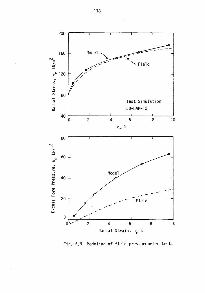
118

200

mgl

Fie1dx2 ’¤ 120 /„; , /

‘Q /L

G; 80ÄE Test Simu1ati0n.16-HAM-12

40 0 2 4 6 8 10er %

80mExZAC

Q 60:

253 Mode13 40Lcx.¤J LL ,, «E L ·

’3 E //’ madcu /0 ° />( Z1.1.1

02 4 6 6 10

Radia1 Strain, EP %


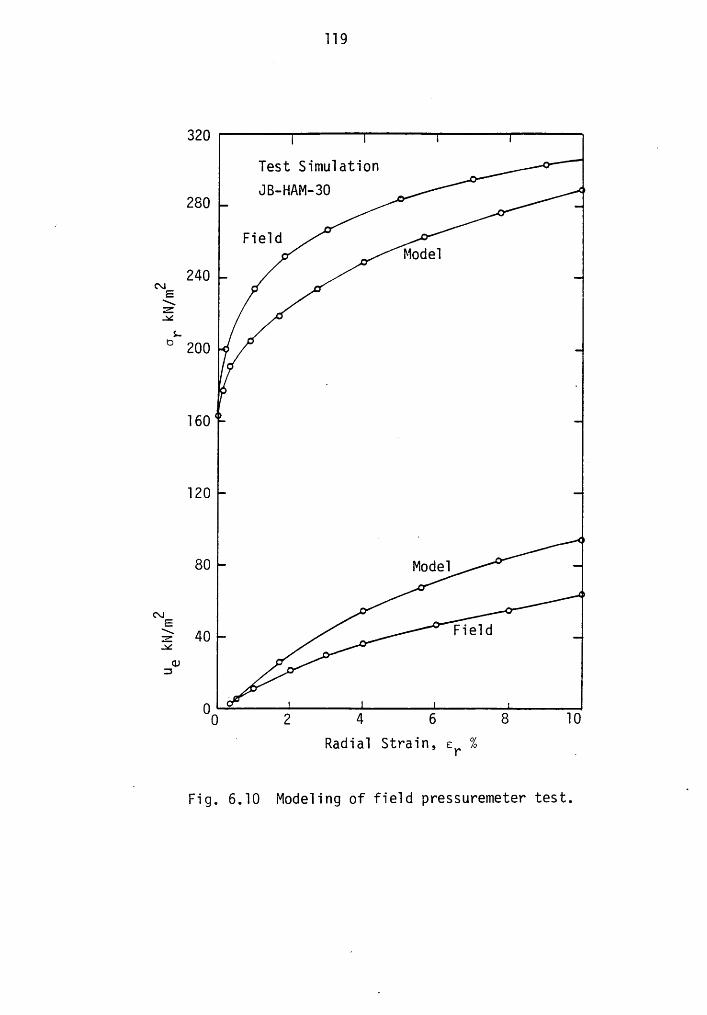
119

320Test Simulation •JB-HAM-30 · ·280 '6 Field ° ·• _ Model

240N • .EErfg •

L .° 200l'

~ ·

160"

120

80 Model 'mE ° °E 40

•Field

3•

00 2 4 6 8 10’ Radial Strain, Er %

1Fig. 6.10 Modeling of field pressuremeter test.

u

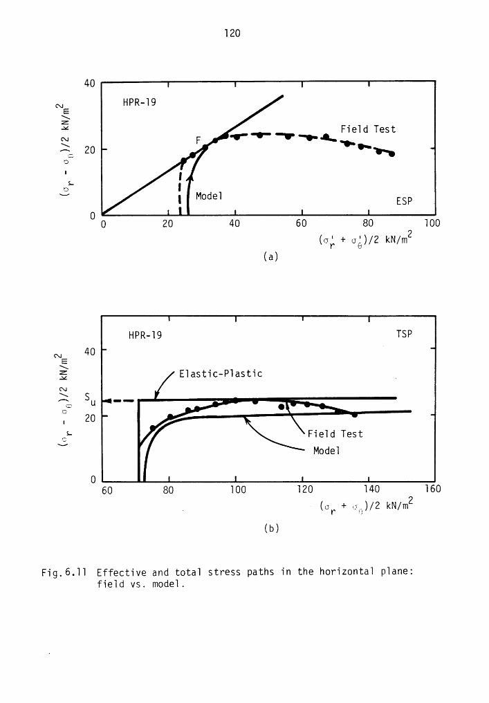
120

40N HPR—19

E\E Fwd TestN F "‘°°°'-_'°‘l•«I—\ ‘Ü••—"‘/_

h

Is.

3 M0de1 ESP0 0 20 40 60 80 100

(6;+ 66.;)/2 kN/m2

(6)

HPR—19 TSPN 40 I

EE1astic-P1astic _

wl SU __ .oc *1 .„ 20CS- Fie1d TestV M0de1

060 80 100 120 140 160

. (dr + d„>/2 kN/m2(b)

Fig.6.11 Effective and t0ta1 stress paths in the h0riz0nta1 p1ane:fie1d vs. m0de1.

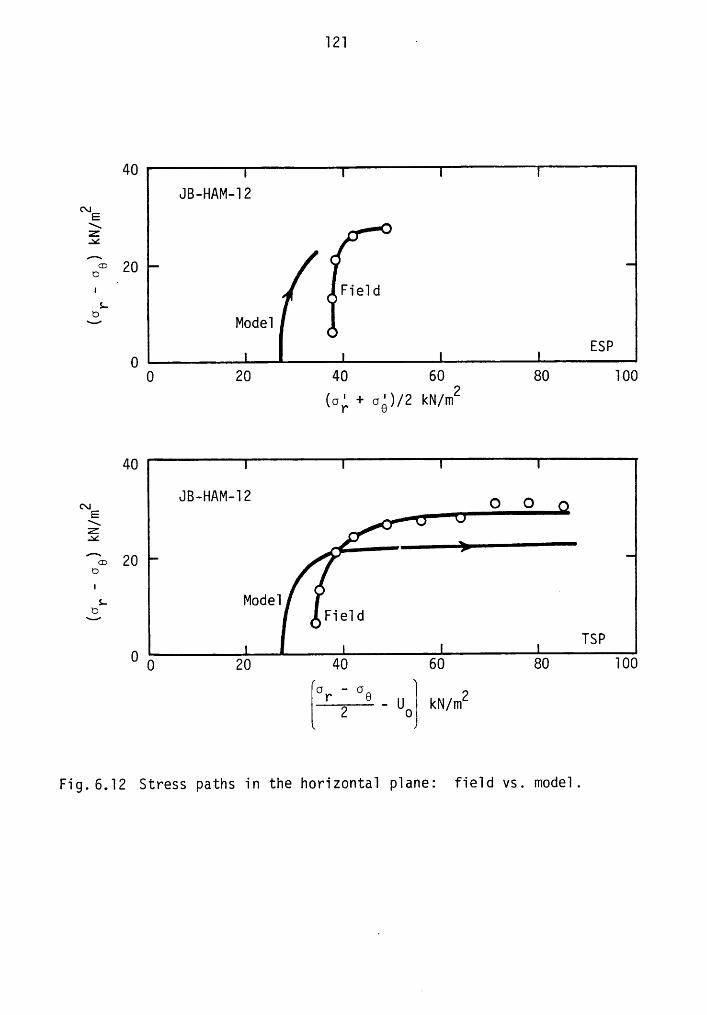
121 ·

40JB-HAM-12

cwE\z..>¢fm 20

• “Fie1dÖs.

~· 2 Mode1ESP

00 20 40 60 80 100

(0]; + sé)/2 kN/m2

40

NE JB-HAM-12 O O •

^.„ 20 °¤I • _

.., Fie1dTSP

O 0 20 40 60 80 1000 — 0r 6 2

Fig. 6.12 Stress paths in the h0v·iz0nta1 p1ane: fie1d vs. m0de1.

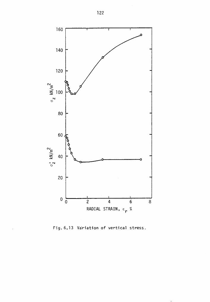
122

160

140

120

~E\§ 100

N¤

80

60

cx:E\E 40— N¤

20 ·

0 0 2 4 6 6RADIAL STRAIN, er %

. Fig. 6.13 Variation of vertica1 stress.

123

stress 6; sharply decreases at the beginning of the test. This is due

in part to the build up of pore pressure due to shearing of the

soil--a phenomenon not manifested by elasticity formulations. The

failure occurs at approximately 2% radial strain whereupon G; assumes

nearly a constant value. That means after failure an increase in

vertical stress is directly transferred to the pore water and no further

generation of pore pressure occurs.

what is surprising is the observation that total vertical stress

62 also goes down as the test begins. It levels off between 0,5 to 1%

radial strain and increases thereafter. Note that at the moment of

failure, close to 2% radial strain, 62 is approximately the same as it

was prior to the commencing of test.

No field records exist to verify Fig. 6.5. However, laboratory

experiments support the analytical observations. As this research

work was underway, Arno Sinram at Stanford University performed cubical

tests on Bay Mud simulating the elastic-plastic pressuremeter loading

path. The results of one of the tests are given in Appendix 4. It can

be seen that the effective as well as total vertical stress decrease

rapidly in the prefailure stage of the test. Similar observations are

reported by wood and wroth (1977) from cubical tests on Spestone kaolin.

Fig. 6.14 demonstrates how the pressuremeter test alters the in-

situ state of stress in the vicinity of the cavity. while the effective

tangential and vertical stresses, 6é and 6;, reduce from their in-situvalues, the effective radial stress 6; rises. The alteration is maximumat the cavity-probe interface and it diminishes rapidly as we go away

from the cavity. No change in stress state is experienced by soil at a

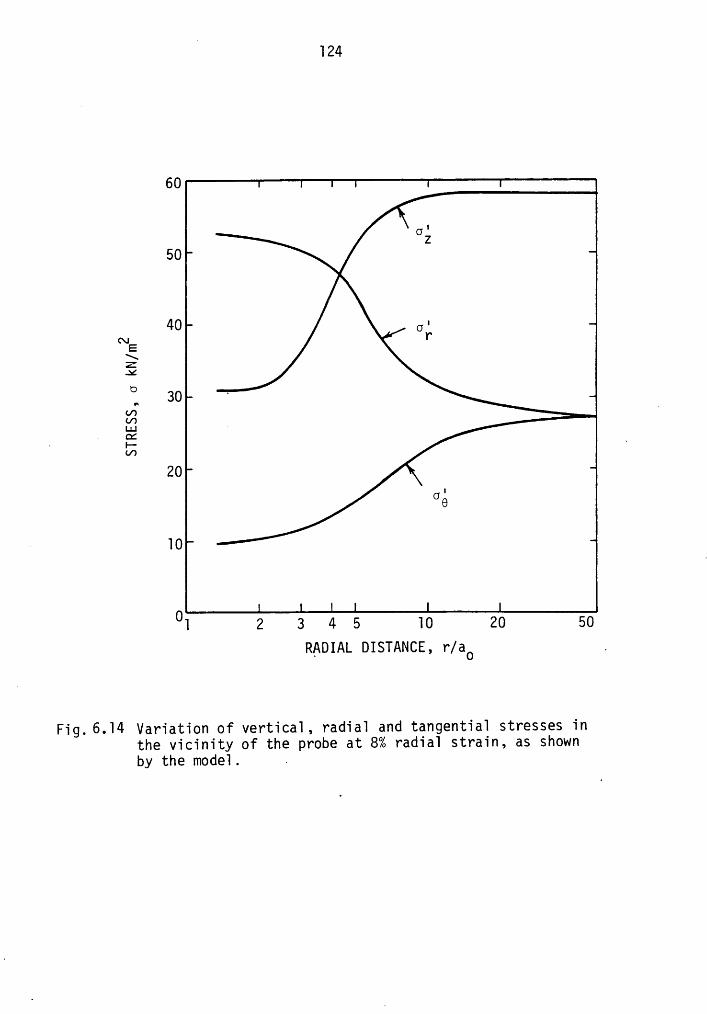
·0

124

60

50

40NEI>ZZ‘j so · .m

. P-_

uv20

V ¤é· 10

0 1 2 3 4 5 10 20 50RADIAL DISTANCE, r/ao .

Fig.6.14 Variation of vertica1, radia1 and tangentia1 stresses inthe vicinity of the probe at 8% radia1 strain, as shownby the mode1. .

l25

distance of 50 times the cavity—radious from the center of the cavity,

suggesting that a finite element mesh of length 5OaO would have

sufficed for the analysis. The difference between the bell-shaped

curves, o; and og, represents twice the shear strength mobilized.

6.3 SIMULATION OF HOLDING TEST

Fig. 6.l5 shows the finite element simulation of the holding test

JB-HAM-30. The test was controlled by applying the loading increments

(or decrements) every half minute, as indeed was done in the field,

and thus, the radial stress vs. time curve was duplicated as closely as

possible. The resulting variation of the radial strain, er, with time

appears to be in good agreement with that recorded in the field.

The development of excess pore pressures occurs at a more rapid

pace in the model than that observed in the field. However, the

dissipation processes in the field and analytical model are in close

agreement. The slower development of pore pressures in the field may

be related to lag in the measuring systems due to non-saturation, a

common problem in the field and the laboratory. All in all, the

comparison is felt to support the analytical simulation procedures.

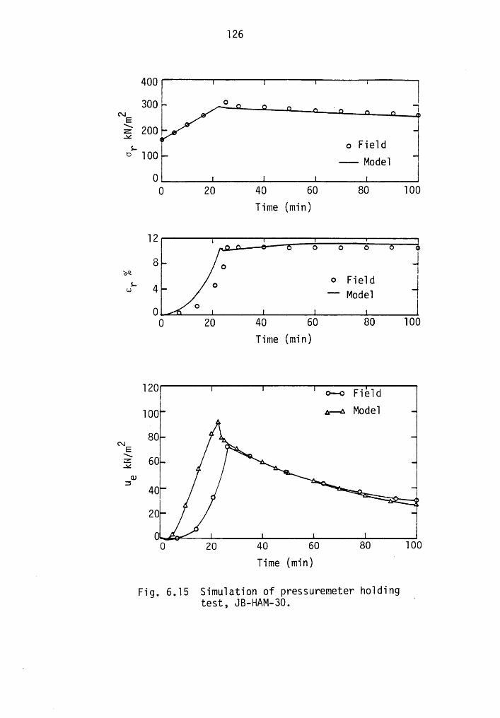
126

400l

300 °5 200Os. 100 o Fie1d

—— Model0

0 20 40 60 80 100Time (min)

12 o o o

S 8 O 1wa 4 O <> Field -4}" ModelO o

0 20 40 60 80 100Time (min)

188 O-O Fieldmg A-6 Model

80C\15E 60sm

4020

00 20 40 60 80 100

Time (min) 8

Fig. 6.l5 Simulation of pressuremeter holdingtest, JB—HAM-30. '

CHAPTER 7

EFFECT OF FINITE PRESSUREMETER LENGTH:

THE AXISYMMETRIC ANALYSIS

In the last chapter, a series of plane strain finite element ‘

analyses were performed and shown to yield good predictions for the

field tests. However, it is reasonable to ask if out¥of-plane effects

can influence the test, particularly the excess pore pressures since

it is possible that vertical as well as horizontal drainage can occur.

Thus, the work for this chapter involves performance of a series of

axisymmetric finite element analyses which consider possible drainage

and pore pressure dissipation effects. These are compared to the

plane strain appraoch to test its validity.

A judicious selection of the element type has to be made if

meaningful results are to be obtained from a FEM consolidation scheme.

Here, the eight noded element, Q8P4, with displacement degree of

freedom at 8 nodes and pore pressure degree of freedom at 4 corner nodes

was used. The variation of displacement along each side of the element

is assumed quadratic while the variation of pore pressure is linear.

Thus, the element is isoparametric for displacement and super-parametric

for pore pressure variables. The Q8P4 element, where the pore pressure

variation is of one degree lower to that of displacements, was found

favorable for two dimensional coupled consolidation problems (Johnston

and Clough, l983). Note that in the preceeding chapter, even though

we used identical shape functions to define the variation of

l27

l28

displacement and the pore pressure within each element, no numerical

difficulties were encountered as the problem was one dimensional

(Carter, Randolph and wroth, l979).

However, the use of a O8P8 or Q4P4 element in a coupled consoli-

dation problem results in a sinusoidal fluctuation of pore pressures

about some mean value which is usually the pore pressure variation

evinced by the O8P4 element. A large number of O4P4 elements have to

be used before a comparison between the three types of two dimensional

consolidation elements can be made; this is not considered here a dis-

advantage of the O4P4 element, given the fact that a quadratic element

requires much higher computational effort than of a linear element.

Fig. 7.l shows the finite element mesh used in the analysis of

the pressuremeter test. A total of l84 O8P4 elements carrying 6l3

nodes are used to define a soil medium which extends a minimum of 5OaOfrom the center of the pressuremeter. ao is the radius of the cavity.

Note that the top boundary of the mesh is not constrained against

vertical displacements for, should the medium consolidate, a vertical

constraint on the upper boundary would throw the entire half of the

mesh into a state of extension.

7.l SIMULATION OF FIELD TESTS

The predicted response for the test JB-HAM—l2 is shown in Fig.

7.2 where the stress-strain-pore pressure curves from the axisymmetric

analysis are compared with those of plane strain analysis and the field

tests. The results predicted for the midplane level of the axisym-

metric analyses are used in this comparison. These is no appreciable

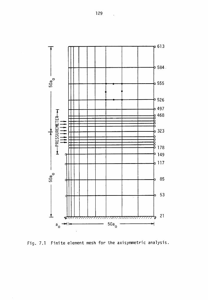
129 _

• 584.3 IIIIIIIII6 IIIIIIIII2IIIIIIKKK2 526IIlll—111' 666

I I-1—_——

- ::=====22-IIKililje .. un-¤—111_ 333a ;·-,_un-nziiiV7

___Il11Äl—--•

ät-'___ II]————QIll-——

6IIIlIlI———6 666•¢O3 IIIIIIIIII. 856 IIIIIIIIIIVVao

—>-1 Ht---- 50aO ——-—————>-1

Fig. 7.1 Finite e1ement mesh for the axisymmetric ana1ysis.

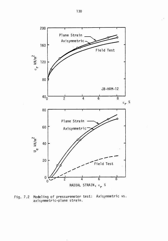
130

200P1ane StrainAxisymmetric

160 _ (” Fie1d Test<\I

E I\f§ 120OL

°/80 · _

JB-HAM-12

400 2 4 6 6.

Er,80

P1ane Strain ° °00 Axisymmetric 2

N • •gg 40

Q) .D

, , ,,·’ Fie1d Test'

ZZ/

0 /0\1’ 2 4 6 8RADIAL STRAIN, er %

Fig. 7.2 Mode1ing of pvessuremeter test: Axisymmetric vs.axisymmetric—p1ane strain.

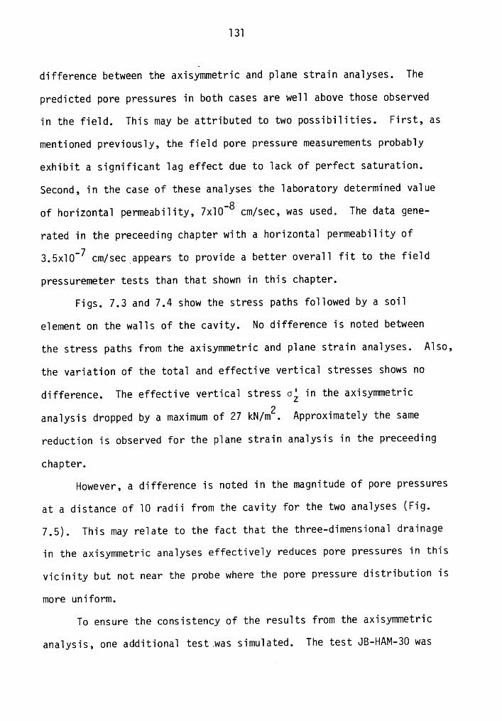
131

difference between the axisymmetric and p1ane strain ana1yses. The

predicted pore pressures in both cases are we11 above those observed

in the fie1d. This may be attributed to two possibi1ities. First, as

mentioned previous1y, the fie1d pore pressure measurements probab1y

exhibit a significant 1ag effect due to 1ack of perfect saturation.

Second, in the case of these ana1yses the 1aboratory determined va1ue

of horizonta1 permeabi1ity, 7x10”8 cm/sec, was used. The data gene—

rated in the preceeding chapter with a horizonta1 permeabi1ity of

3.5x10”7 cm/sec appears to provide a better overa11 fit to the fie1d

pressuremeter tests than that shown in this chapter.

Figs. 7.3 and 7.4 show the stress paths fo11owed by a soi1

e1ement on the wa11s of the cavity. No difference is noted between

the stress paths from the axisymmetric and p1ane strain ana1yses. A1so,

the variation of the tota1 and effective vertica1 stresses shows no

difference. The effective vertica1 stress og in the axisymmetric

ana1ysis dropped by a maximum of 27 kN/mz. Approximate1y the same

reduction is observed for the p1ane strain ana1ysis in the preceeding

chapter.

However, a difference is noted in the magnitude of pore pressures

at a distance of 10 radii from the cavity for the two ana1yses (Fig.

7.5). This may re1ate to the fact that the three-dimensiona1 drainage

in the axisymmetric ana1yses effective1y reduces pore pressures in this

vicinity but not near the probe where the pore pressure distribution is

more uniform.

To ensure the consistency of the resu1ts from the axisymmetric

ana1ysis, one additiona1 test was simu1ated. The test JB-HAM-30 was

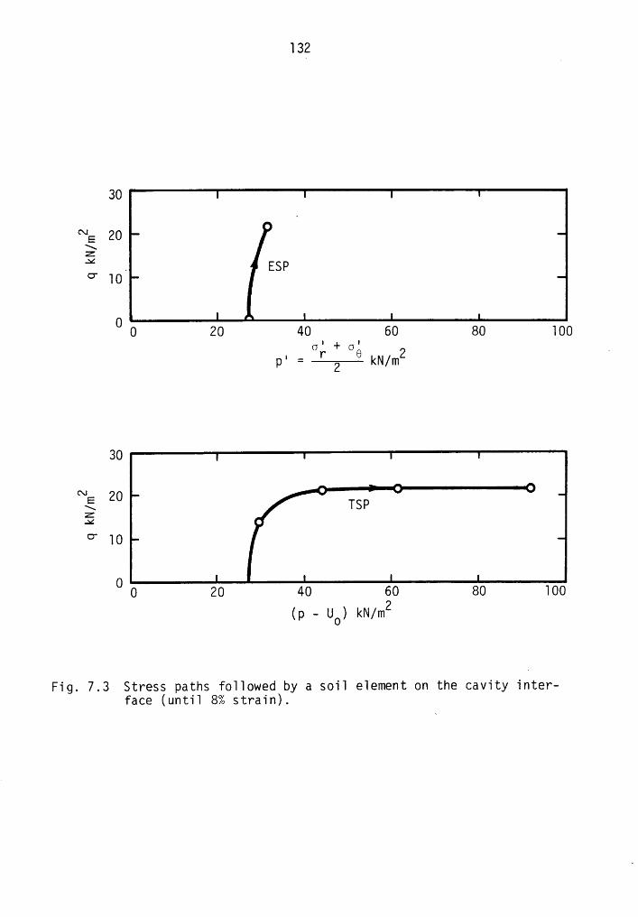
132

30

NE 20 °\E . ESP°” 10

0 20 40 60 80 100GI + Ol V

30

Q] Q O O

E 20 ispz¥ •

O- 10

O 0 20 40 60 80 100(p - 00) kN/m2

Fig. 7.3 Stress paths f0110wed by a s0i1 e1ement on the cavity inter-face (unti1 8% strain).

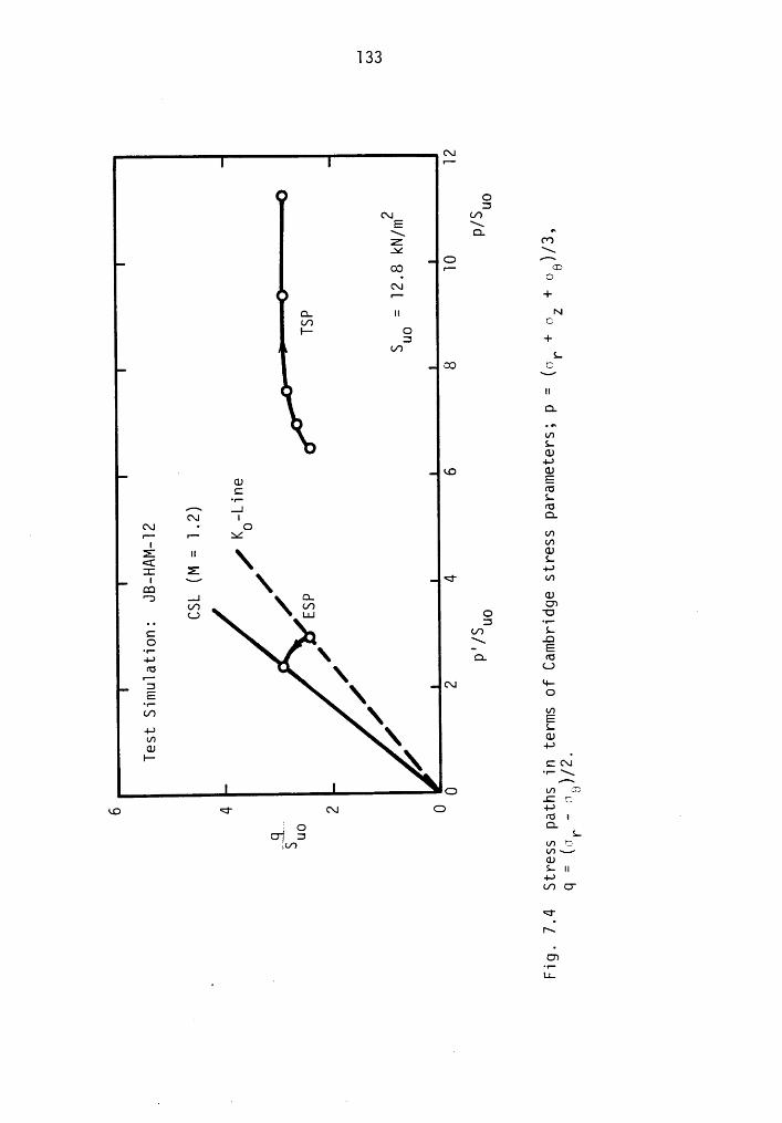
(\Ir-·

O3

C\I (/7

Ü¤_ •~

Q /%CO r— QD• O(\I«— +

Q. II N(/7 CI-- O

3 +V7 L

CO C\-Z

IIQ.

U')LQ)

+-7· (O CD

Q) EC (U

•¤- Lrx _] (UC\I I Q.

<\I · O‘ r·—· r- bd (/7I I/7

E n cu<[ L1 Z 4-:

I L-\

Ü If)E"D .-I D. GJ(/7 V7 U7

L) LI.! C Ü.• 3 „,.„

C • V7 LGN+-7\ D. (U

rt: 0 \L.)

1-··3 cx: *4-E \ 0·•—an \

anE4.: LIn \ GJQ) -I-7I., •

CC\Ixs

G (/7 G.C C

KO <I' AI G P_ (Ö I ·: Q Q.¤1 = L

CDL IIP(/7 Ö-

ÜI\

C7-r-

Ä LL

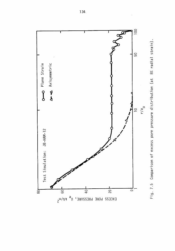
134

„ GlgO

O• z;• E

FUS fs• S; WT6

<: U ° E°|* 'Y"rc: s.. S-is- 4(1 ‘ EQ

OOO

anE >” 4—·2 L 4 J3Ä <>E • ‘

äil · 4:6 ° EE• < 4-*

OC)r¤ 'Or-•[ L E

an</3

ILCLC: Iä;• Q.ZE /Ä g(I)

IÜ Q)

OIä* ·+--„— ‘ 0

4-* I2 ä:: _V*.E 4 EJ) ° g4,; // ä2 • L’

‘ LO

@N

© G GGI- I\

ZW/11*1 {1 ‘3Hf1SS38d 3HOd SSEIOXH LL

l35 .

now selected since the test was located in the overconsolidated zone of

Bay Mud. The comparisons are shown in Fig. 7.6. Again, differences

between the axisymmetric and plane strain analyses are insignificant.

7.2 OBSERVATIONS IN THE VERTICAL PLANE ‘

Thus far we restricted our attention to the horizontal plane

passing through the mid-height of the expanding membrane, where the

feeler strain gages are situated. It is also of interest in the case

of the axisymmetric analyses to examine the deformation patterns and

the distribution of pore pressures along the entire length of the

pressuremeter.

Fig. 7.7 shows the displacement vectors for the test JBQHAM-l2

at 8% radial strain at the cavity wall. A magnified picture is pre-

sented in Fig. 7.8. It is seen that the soil at the mid-height of the

probe does deform in a plane strain mode. Hartman and Schemertman

(l975) reached a similar conclusion from a nonlinear elastic finite

element analysis on sands under fully drained conditions. No consoli-

dation elements were used in their analysis.

Fig. 7.9 shows the contours of percentage strength mobilized.

As evident, only an annulus with thickness ao has reached criticalstate at 8% radial strain on the face of the cavity.

A unique outcome of this analysis is given in Fig. 7.lO where

the contours of excess pore pressure are drawn. Two observations can

be made. First, the flow of water at the mid-height of the probe takes

place radially in the horizontal direction. This is encouraging inas-

much as such a condition is assumed to exist in the plane strain

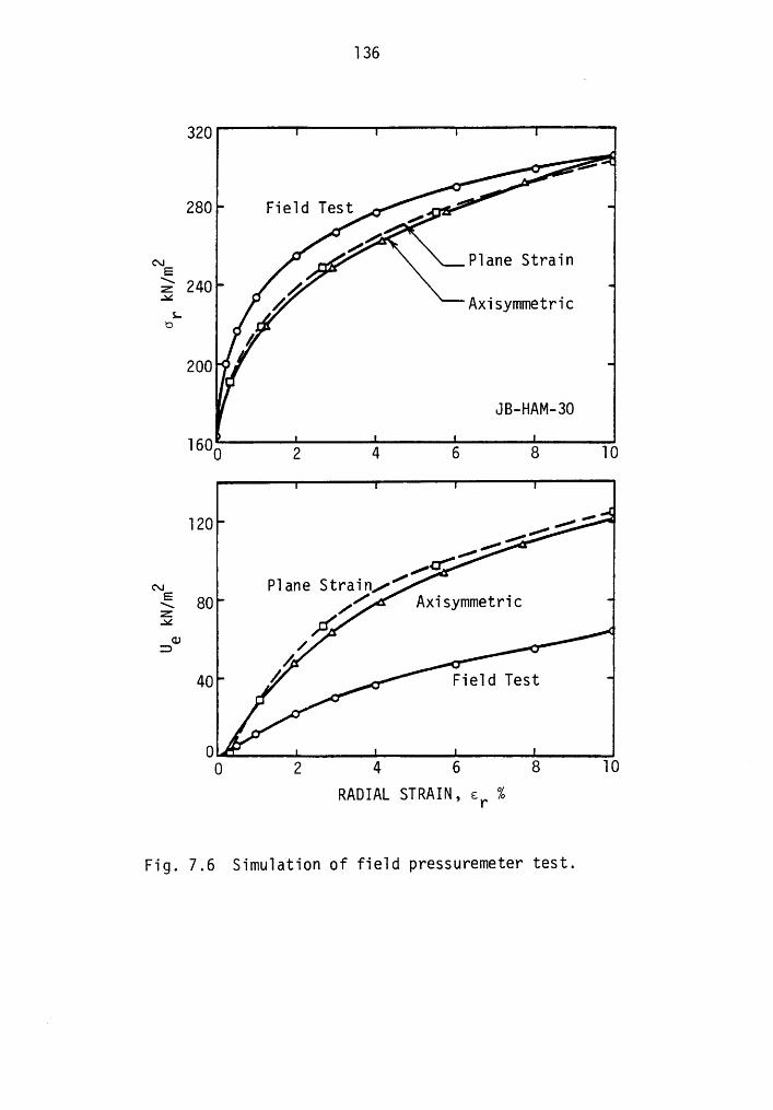
136

320• Ä :

280 , ,_

NE ° «. P1ane Strain

E 240 _E Axisymmetric

D • [L

ZOO '° 6” JB-HAM-30

1600 2 4 6 8 10

120 //z’ ‘«»cÜ'

GJ P1ane Stra1n,»"5 80 /EE A OE / •

O40 / .

0 Z'•

0 2 4 6 8 10RADIAL STRAIN, Er %

Fig. 7.6 S1mu1at10n of f1e1d pressuremeter test.

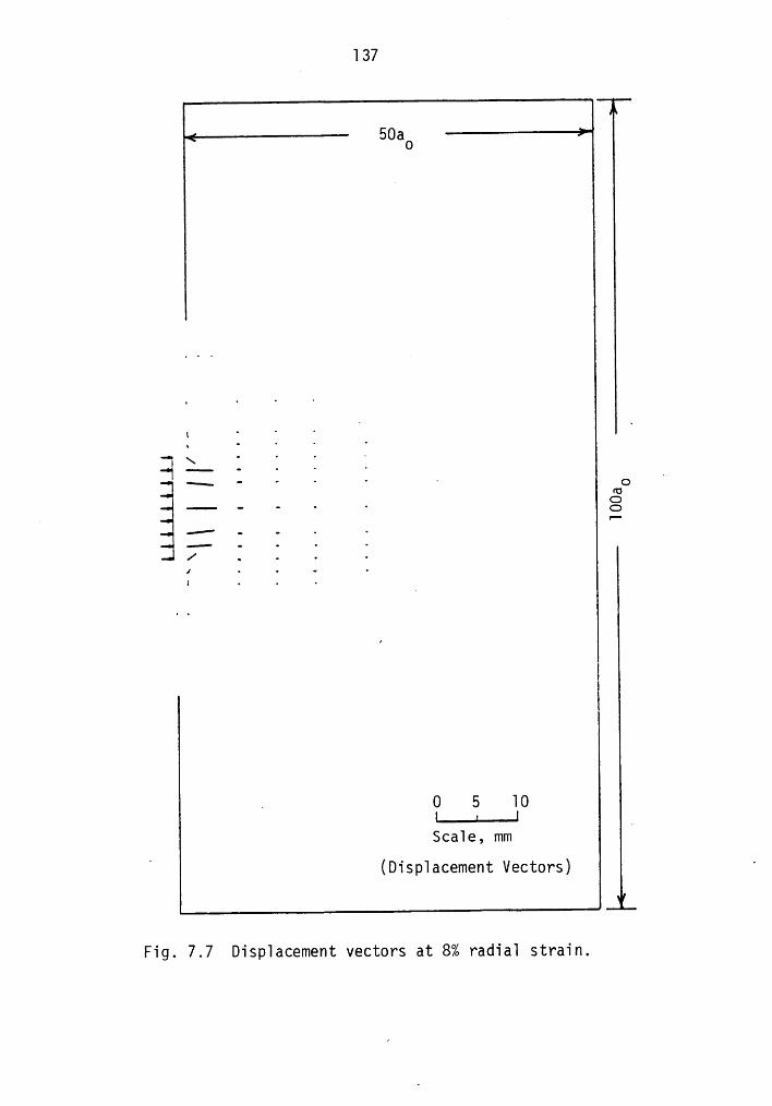
137

50a

‘

0

gi. Ä•

° ° ' ' QU

ruO

Ä I Ä Z

. 0 5 101.....:...-I _Sca1e, mm

1(Ü1Sp1äC€1I’1€|'1t V€CtOY‘S) '

Fig. 7.7 Disp1acement vectors at 8% radia1 strain.

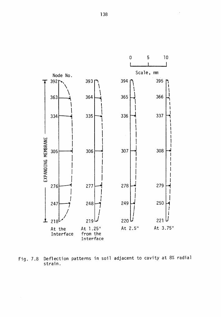
136 ·

0 6 IOI._._I..ZI

Node NO' ScaIe, mmg392 „ 393 394 395\ \ I 1

\ I I363 364 365 I 366I I 1I 1 I I334 335 336 337

1 1I 1 1 11..1.1 I I IZ<: I I I Igg 15 305 306 307 308E

I I I Ies I I IE I 1¤ I IZ I

ä 1 I 1 ‘L11 I

276 277 278 279I 1 I 1I I I247 248 249 I 250 1

/ / 1 1216 219 220 221At 1116 At 1.26·· At 2.6·· At 3.76··Interface from the

Interface

Fig. 7.8 DefIect1on patterns in so1I adjacent to cavity at 8% rad1aIstrain.

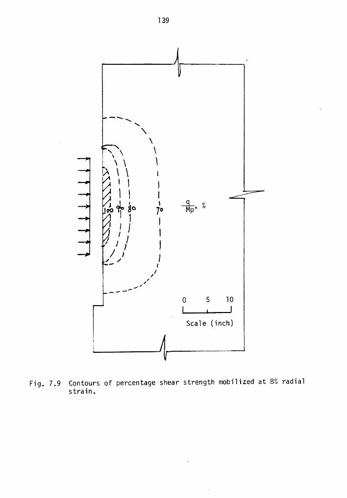
139

\\

1\\ 1111 19111 1

111 1‘ 1 ..q..¤1·· MW

I1 1,1) 1/1 I/'/

° I/

1 1/

0 5 101

1...lL.-J

Sca1e (inch)

1

1

Fig. 7.9 Contours of percentage shear strength mobi1ized at 8% rad1a1strain.

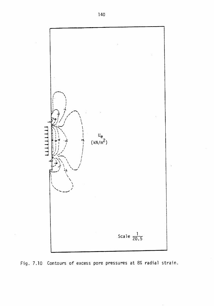
l40

\‘1I I{ 1

II J5 1,/ \ I I

1 /1 1 \ ·/ / I••§ ll; / [ ‘

\=<·’ 1I _I I I \~ I UE-

‘ s +1,j I?II °f 1 (kN/m2){ 1 I I I1 1 / 1

I

\ ai ,

__1 "’I \I \\ 1\\ /~-../

I IScale J-20. 5 .

Fig. 7.lO Contours of excess pore pressures at 8% radial strain.

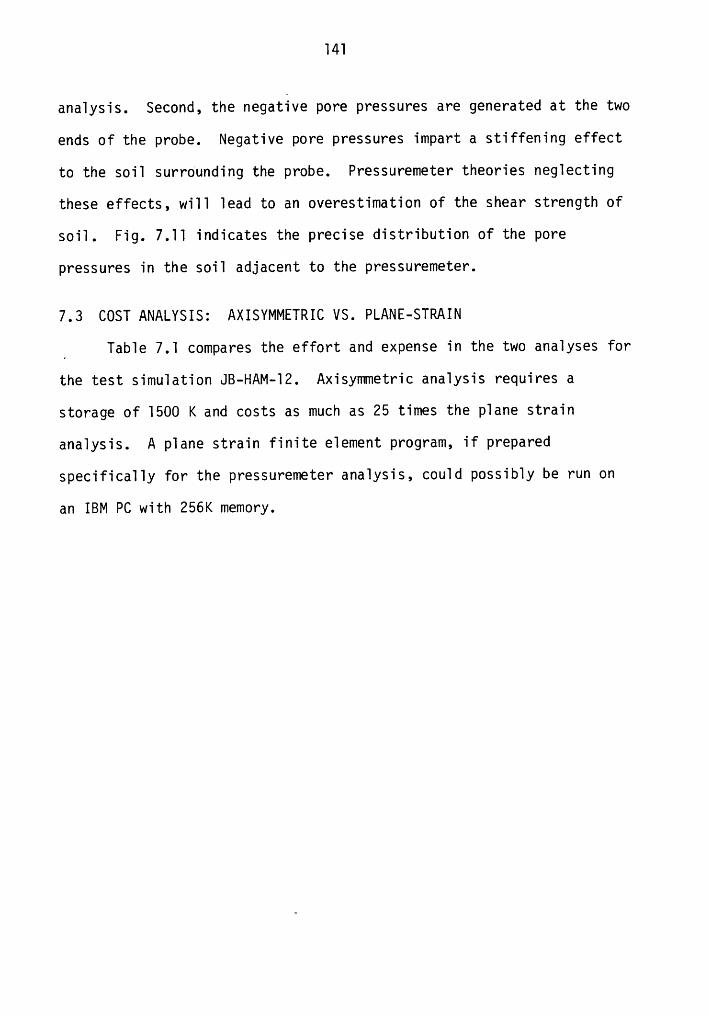
l4l

analysis. Second, the negative pore pressures are generated at the two

ends of the probe. Negative pore pressures impart a stiffening effect

to the soil surrounding the probe. Pressuremeter theories neglecting

these effects, will lead to an overestimation of the shear strength of

soil. Fig. 7.ll indicates the precise distribution of the pore

pressures in the soil adjacent to the pressuremeter.

7.3 COST ANALYSIS: AXISYMMETRIC VS. PLANE—STRAIN

_ Table 7.l compares the effort and expense in the two analyses for

the test simulation JB-HAM-l2. Axisymmetric analysis requires a

storage of l5OO K and costs as much as 25 times the plane strain

analysis. A plane strain finite element program, if prepared

specifically for the pressuremeter analysis, could possibly be run on

an IBM PC with 256K memory.

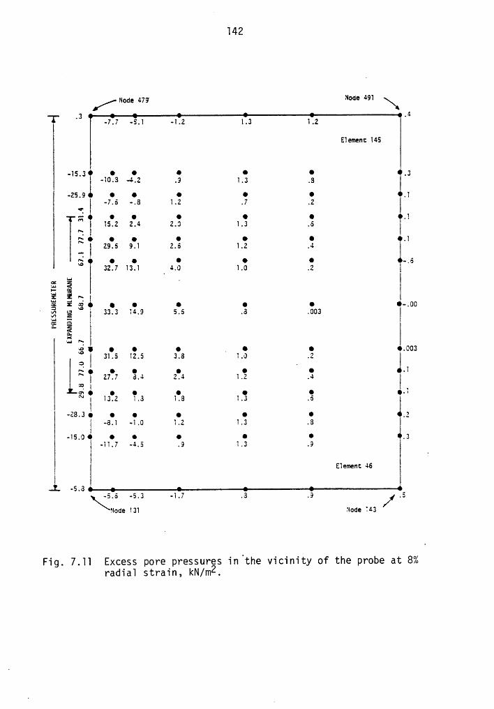
142

’/- Mone 47; N¤d¢ 491 \g.3 .4-7.7 -5.1 -1.2 1.3 1.2

E1ement 145

•1§_3 Q Q Q Q Q- _3-10.3 -4.2 .9 1.3 .8

-25.9 • • • • • ,1-7.6 -.8 1.2 .7 .2"Z(7; Q Q Q Q Q .115.2 2.4 2.0 1.3.6'TQ Q Q Q Q Q Q .1I 29.6 9.1 2.6 1.2 .4 Ig • • • • • -,5

32.7 13.1 4.0 1.0 .2 ILA

1_

E ä1: ä vgg Z g l Q Q Q Q Q -.00‘ gg <__-E 33.3 14.9 5.6 .3 .003

I; E- E I><“" 'TLg Q Q Q _ Q Q Q.003I 31.5 12.5 3.8 1.0 .2 IQ .g; • • • • • -1

_ 27.7 3.4 2.4 1.2 .4°“? Igg • • • • Q -113.2 1.3 1.8 1.3.2:-28.3QQ Q Q Q Q ,3-8.1 -1.0 1.2 1.3 .8

-15.0 • • • • • _g-11.7 -4.5 .9 1.3 .9

E1ement: 46

..7. -5.3 Q.6 -5.3 -1.7 .3 .9 .5Mode 131 Node 143

Fig. 7.11 Excess pore pressures in the vicinity of the probe at 8%radia1 strain, kN/m2.

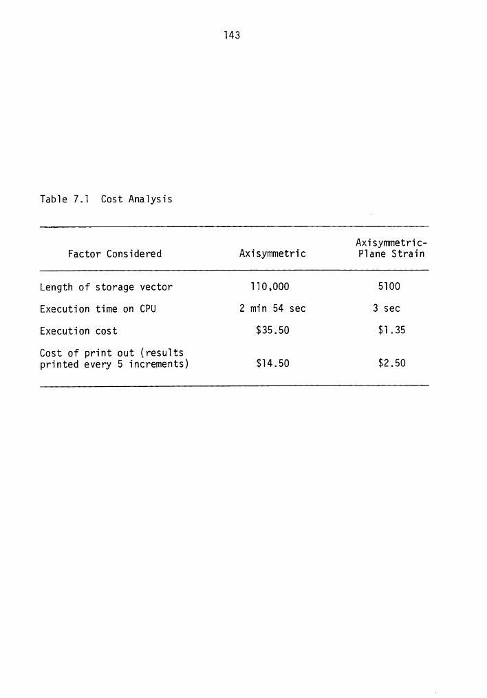
143

Tab1e 7.1 Cost Ana1ysis

Axisymmetric-Factor Considered Axisymmetric P1ane Strain

Length of storage vector 110,000 5100

Execution time on CPU 2 min 54 sec 3 sec

Execution cost $35.50 $1.35

Cost of print out (resu1tsprinted every 5 increments) $14.50 $2.50

· CHAPTER 8

DRAINAGE DURING SHEAR IN THE PRESSUREMETER TEST

To this point in the thesis the major question of the work,

namely, at what rate of loading does drainage occur in the pressure-

meter test, has not been addressed. The previous two chapters have

shown that: (l) The plane strain model of the pressuremeter problem

reasonably simulates the mid—plane response; and, (2) the pressure-

meter curve can be accurately predicted by the model although the

analytic pore pressures are generally higher than the values observed

in the field. In regard to the latter issue, we may postulate that

either the permeability used in the analyses is too low (thereby not

allowing enough drainage), or that there is a time lag effect in the

measurements. There is no way to know exactly which of these two

possibilities is correct, but some insights can be gained by further 4

analysis.

8.l EFFECT OF PERMEABILITY IN MODELING ACTUAL TESTS

One technique to check the effect of permeability is to determine

its influence in light of actual test results. For this purpose, tests

JB-HAM-lO and JB-HAM-l2 were analyzed. These were chosen since both

total pressure results and pore pressures were successfully monitored.

In the analyses, permeability is varied from the value obtained as a

horizontal permeability in the laboratory (7xlO”8 cm/sec) to 5 and 2O

times this value. In his field holding tests, Benoit (l983) found

that it was about 5 to 8 times the laboratory value.

I44

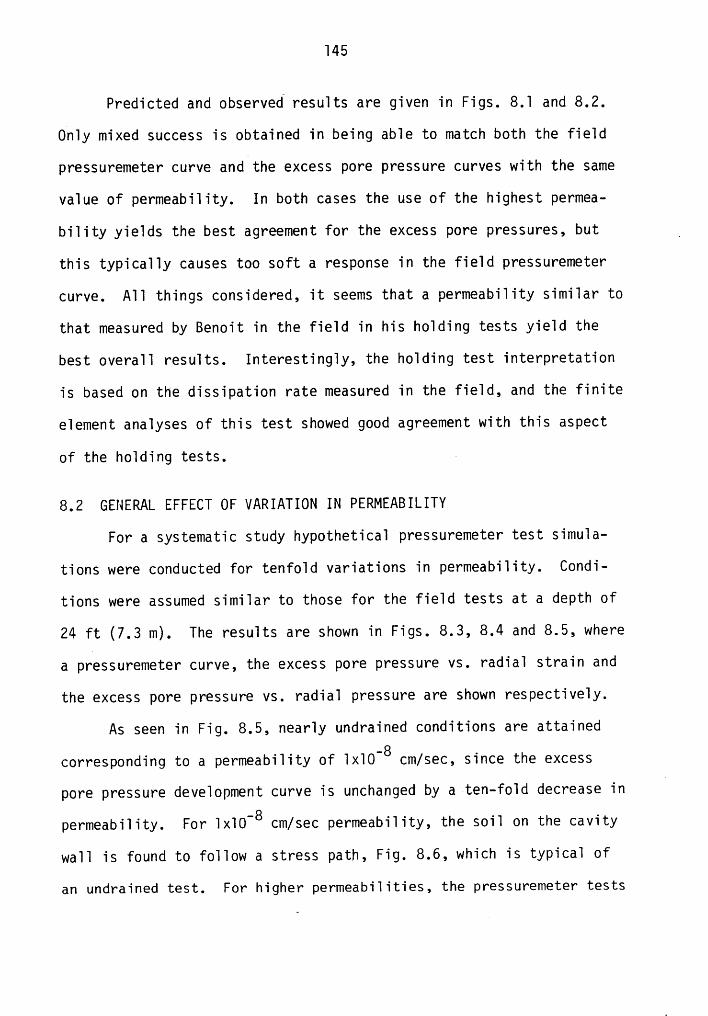
145

Predicted and observed resu1ts are given in Figs. 8.1 and 8.2.

On1y mixed success is obtained in being ab1e to match both the fie1d

pressuremeter curve and the excess pore pressure curves with the same

va1ue of permeabi1ity. In both cases the use of the highest permea-

bi1ity yie1ds the best agreement for the excess pore pressures, but _

this typica11y causes too soft a response in the fie1d pressuremeter

curve. A11 things considered, it seems that a permeabi1ity simi1ar to

that measured by Benoit in the fie1d in his ho1ding tests yie1d the

best overa11 resu1ts. Interesting1y, the ho1ding test interpretation

is based on the dissipation rate measured in the fie1d, and the finite

e1ement ana1yses of this test showed good agreement with this aspect

of the ho1ding tests. 7

8.2 GENERAL EFFECT OF VARIATION IN PERMEABILITY

For a systematic study hypothetica1 pressuremeter test simu1a—

tions were conducted for tenfo1d variations in permeabi1ity. Condi-

tions were assumed simi1ar to those for the fie1d tests at a depth of

24 ft (7.3 m). The resu1ts are shown in Figs. 8.3, 8.4 and 8.5, where

a pressuremeter curve, the excess pore pressure vs. radia1 strain and

the excess pore pressure vs. radia1 pressure are shown respective1y.

As seen in Fig. 8.5, near1y undrained conditions are attained

corresponding to a permeabi1ity of 1x1O-8 cm/sec, since the excess

pore pressure deve1opment curve is unchanged by a ten-fo1d decrease inE

permeabi1ity. For 1x1O”8 cm/sec permeabi1ity, the soi1 on the cavity

wa11 is found to fo11ow a stress path, Fig. 8.6, which is typica1 of

an undrained test. For higher permeabi1ities, the pressuremeter tests

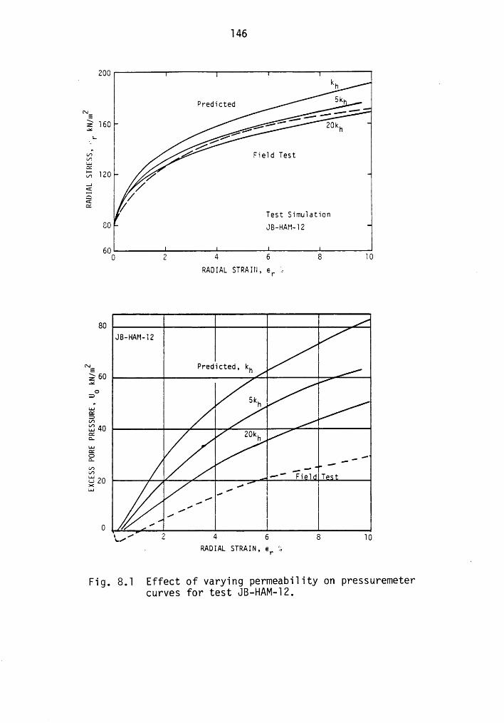
146

200kh .

PredictedNE

§§ 160 20khVLg§ Faeid iesz

E!ä120E //ETest Simulation

80 JB—HAM—l2600 2 4 6 8 l0

RADIAL STRAIN, er X. _

8Q

_

"NE Predicted,khE60 -¢ ,„

O3

.51

m40 [ ' 'E2L/7 .g

{

O ‘„,’ Z 4 6 8 l0„ RADIAL STRAIN, Gr 3

Fig. 8.l Effect of varying permeability on pressuremetercurves for test JB-HAM-l2.

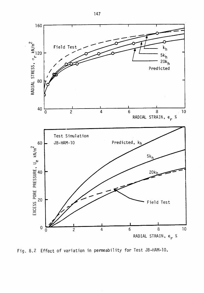
147

1604

.--2

cx: 1•

’ § Fie1d Test/_//• U I kh

• •·U/

U; /~ • • • 20khPredicted

*1 OO)uu ’ //_, 80 V •Q .<E°‘ •

40 0 2 4 6 8 „ 10RADIAL STRAIN, er %

Test Simu1ation _60 JB-HAM—10 ° Predicted, kh

NE

Ex„ cu:

Ew -,«·’an aLLJMcs.LuM

20m Fie1d TestEtiu.:

0 6 2 4 6 6 10RADIAL STRAIN, er %

Fig. 8.2 Effect of Variation in permeabi1ity for Test JB-HAM—10.

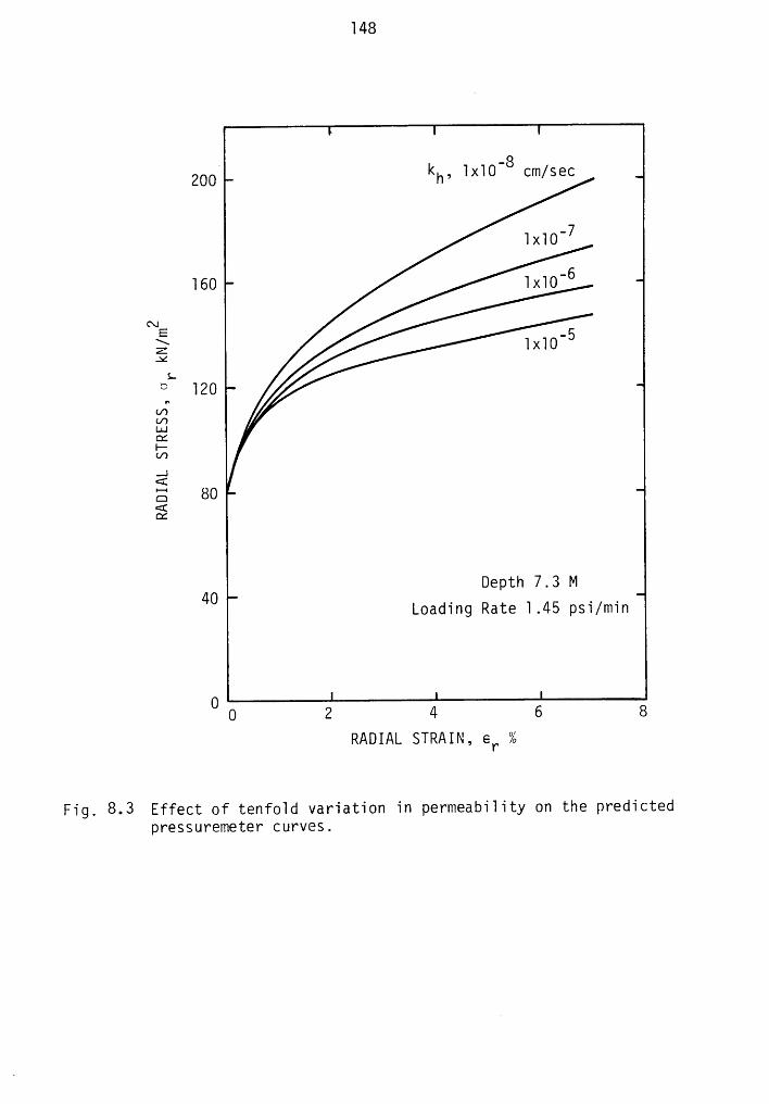
148

20O” kh, 1x10-8 cm/sec

1x10”7160 1x10-6

NEE 1x10°5x

s.8 120V?an1.1.1ocI-</1..1<Z; 80<EQt

40 Depth 7.3 MLoading Rate 1.45 psi/min


Fig. 8.3 Effect of tenfo1d variation in permeabi1ity on the predicted|DY‘€SSUY‘€TT1€t€Y‘ CUTVGS .

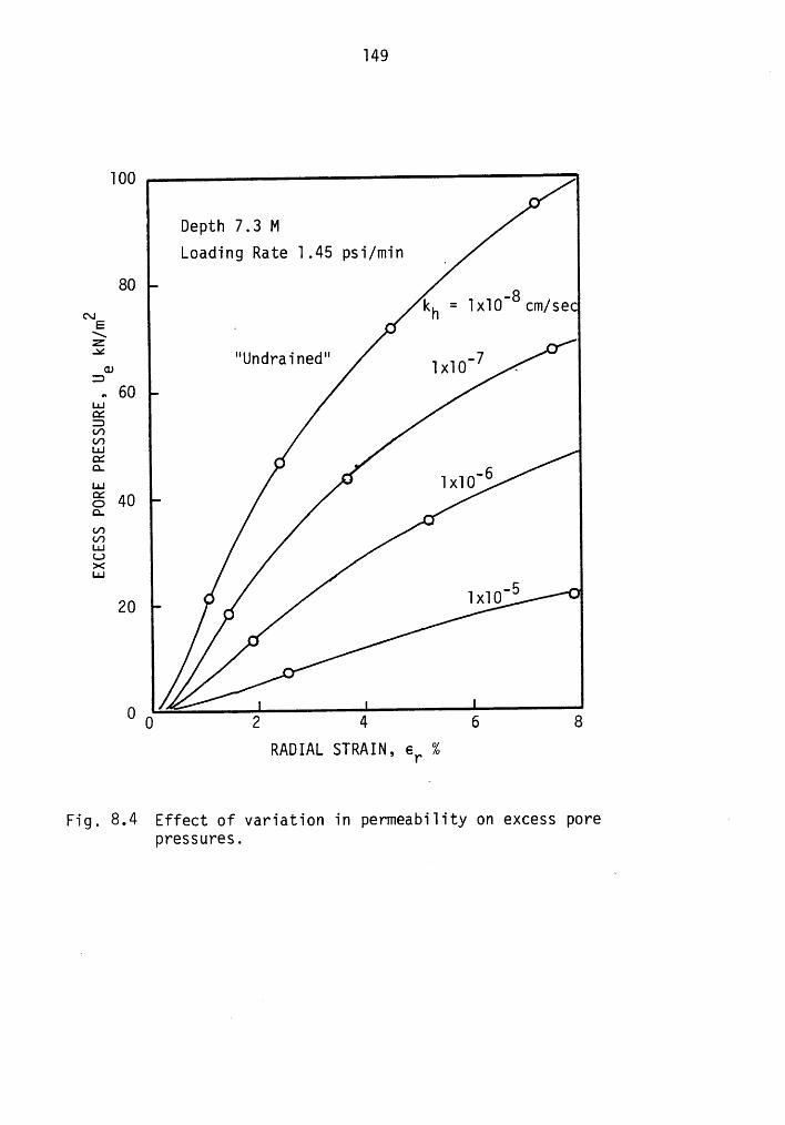
149

100

Depth 7.3 MLoading Rate 1.45 psi/min _

80 8cvE kh = 1x10- cm/se’

. •

G"Undra1ned"Z)„ 60 4

LL!CZDU)U)LuäM · 1x10‘62% 40CL •L/7U')LLJLJ><LIJ

•20 •

•

•


Fig. 8.4 Effect of variation in permeabi1ity on excess pore ~pY‘€SSUY‘€S .

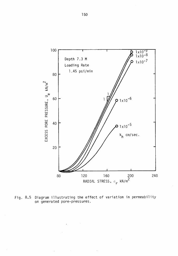
150

100 1: 1x10“éDepth 7.3MLoadingRate X

801.45 psi/min

GIE\ZgcECU 1

„; 60 1 • mo'6MD .(/7(AL1.1MoeLJ.1ää 40 _5¤- ° 1x10<./>E k cm/secQ h '>«Lz.1

20

80 120 160 200 240RADIAL STRESS, or kN/m2

Fig. 8.5 Diagram i11ustrating the effect of variation in permeabi1ityOU Q€T1€Y‘öt€d DOY‘€··pY‘€SSUY‘€S.

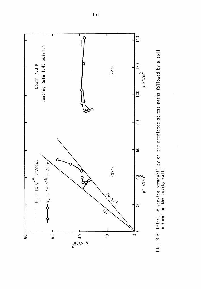
G<I'r-

C·r—E ZI./'I¤ rcs

GZ Q va c\1 >»-

r—· .@PO(\I|\ CU ,2 E Q)

E Z )¤am ‘¥ Ä:G)G C7 Q- LEC 0'O .:fü '—.;.>O rc——)Q.tf)U7G)L4-)<./7

(% ”UG)4-)U••—'OG)LQ.

E .Ggg 4-*

CO_ O

L) U • 3)(1) G) m .,-m In _ „... .\ • .E E ä EZ

G)G LO•

• E3I I ·„ 5__>gGGQ

fiQ.-X X - >'— '—

Cl Ü7füIl II.>„Q)J: -C ÄO L.:—¥ CC Q fü-I->—} cx: >

J) oJ 4-)4-)CUG)(UE¢!—G)

LO-r—LUG)

GRO0 0 0 G C .CO LO <!' (V cg

LU L) •Z /N)| Ü·v—' LL

152

experience a partia1 drainage for the imposed 1oading rate of 1.45

psi/min.An

interesting outcome for these ana1yses is shown in Fig. 8.7

where the subtangent method is app1ied to obtain a stress—strain

response pretending that no drainage occurred in any of the tests.

There is a significant reduction in the interpreted shear strength as

the permeabi1ity increases and drainage occurs in the test.

A simi1ar trend was obtained from the simu1ation of 5 of Denby's

tests for varying permeabi1ity, Fig. 8.8. The tests cover depths of

17.3 to 49.1 ft (5.3 to 15 m). The decrease in pressuremeter shear

strength for a tenfo1d increase in permeabi1ity is again 5 kPa for the

tests in norma11y conso1idated c1ay but is higher in the over-

conso1idated region. Note that the resu1ts shown in Fig. 8.8 are for

a fixed 1oading rate of 1 psi/min.

· 8.3 EFFECT OF RATE OF LOADING ·Fig. 8.9 shows the shear strength profi1e of Bay Mud as obtained

by Denby (1978) and Benoit (1983) from their se1f—boring pressuremeter

tests for the 1oading rate of 1 psi/min. Now the question is, how this

profi1e wou1d have changed had the tests been carried out at a dif-

ferent rate of 1oading? If the reported fie1d tests are indeed un-

drained, then increasing the rate of 1oading shou1d not affect the

computed shear strength since the mode1 does not account for rheo1ogic

or viscous effects. However, if the 1oading rate of 1 psi/min does

permit some drainage during the test, then an increase in the 1oading

rate wi11 1ead to a reduction in drainage, and consequent1y, the

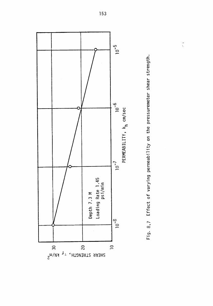
153

II- M'cIC

.C4-*O)CQ)L4-*U)

LfüQ).Cm „LQ)

4-*Q)gg E• ' UQ) 3

U) U)

E QJU L

Q..C

X (D.C•~ 4-*

>-|-— C•—• O..I•*"• >sQ 4-*< *4*L1.] 1--*4-Z .¤ä EN

O•G

P1 Q,

Q.U)

LO C<r ·¤··•C >s1—·r·· S-

E FU

z +°Ü•\ >'|*rum '·4—

00 Z Q. ON U) 4-*

C L)_:·1··· (U

-4-> ·¤ *4-¤. cc *4-Q) O |-4JQ ..I

CO1 NI

‘ICU)

'|"L1.

CD G CD00 t\1 4—·

} ¢Zw/N*1 l H.L5NE1H.|.S HVEIHS

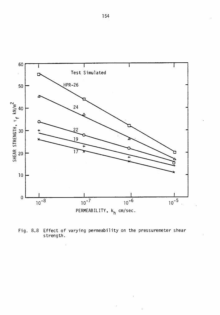
154 _

60. Test Simu1ated

gg HPR-26

aw§ 40 2432

9-[-• ‘ „

ä gg +_ 22ZE;

19 ·I-‘/7 +°‘ 17V1 .

10

0 10-8 10-7 10-6 10-5 . _PERMEABILITY, kh cm/sec.

Fig. 8.8 Effect of varying permeabi1ity on the pressuremeter shearstrength. ·

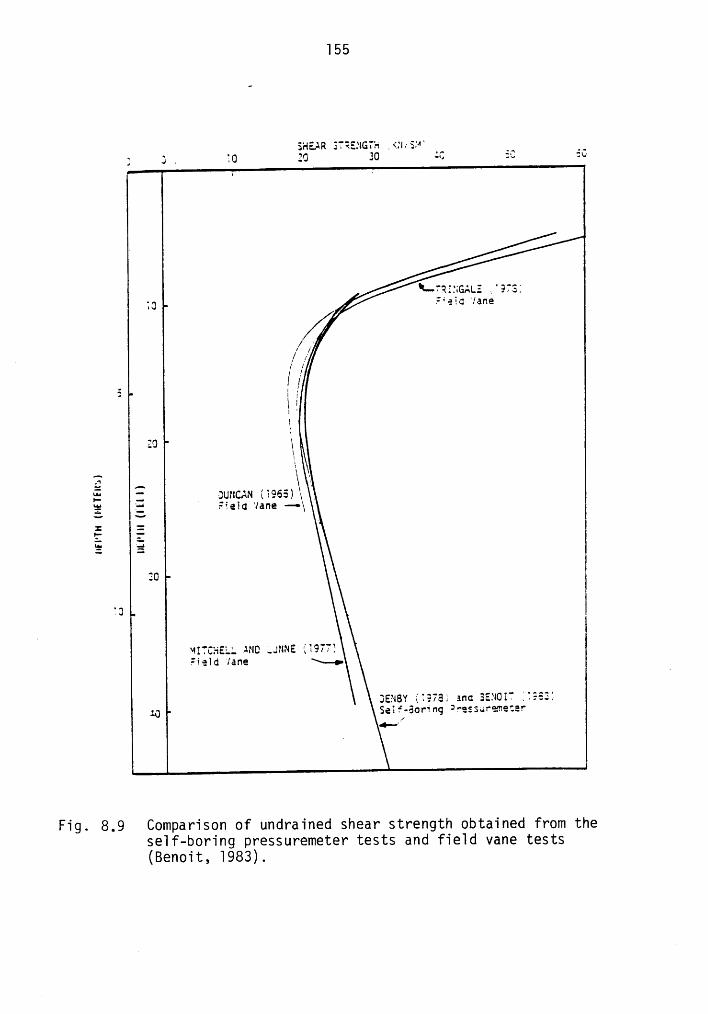
155

SHE.-XR STTEDIGTH ‘K.tI„·Si·" A _« __3 J I jo gg }O ll, Z; ZU

¥-TQZDZGALE ..1275}Field Jane/

11Z l .

„ä1

JUNCÄN' ::1€1d‘]äf1€ —•\

1:*E

TO 1

TWITCHELL -1NO ;.1NNE (1977)Field ‘/ane \-•

JENBY @2732 anc SENOIT ;Ü233ESé1F··3oring 2r·e,S3ur=£¤€§2r6--/

Fig. 8,9 Comparison of undrained shear strength obtained from these1f—boring pressuremeter tests and field vane tests(Benoit, 1983).

l56

pressuremeter will encounter a stiffer soil system. Hence, with the

increasing loading rate the strength profile should be expected to

move rightward until after at some loading rate no further shifting of

the profile would occur whereupon the undrained conditions would be

attained. And, this is the loading rate we wish to determine.

To do so analytically, each of five of Denby's tests, covering

depths of 5 to l5 meters, was first modelled at the field testing rate

of l psi/min. A constant value of horizontal permeability, 3.5xl0°7

cm/sec is used in modeling all five tests. The resulting strength

profile is shown in Fig. 8.lO where it is compared against the strength

profile obtained by the field tests. Note that the experimental

strength profile, as shown in Fig. 8.l0, is a best fit of over 30(

pressuremeter tests (and not just an outcome of 6 pressuremeter curves,

shown in Chapter 6, against which the validity of the model is

checked).

The analytical simulations were then run for different loading

rates. The resulting pressuremeter curves for the test simulation

HPR-l9 are shown in Fig. 8.ll. The generated pore pressures are shown

for the test HPR-22 in Figs. 8.l2 and 8.l3. The pore pressures are

seen to stabilize at the loading rate of 6 psi/min. (A slight increase

in the pore pressures continues due to the numerical approximations

involved.)

Fig. 8.l0 shows the shear strength profiles corresponding to dif-

ferent loading rates. The optimum loading rate for Bay Mud is deter-

mined as 6 psi/min. It may be noted that the shear strength at this

loading rate is approximately l5% higher than what has been reported

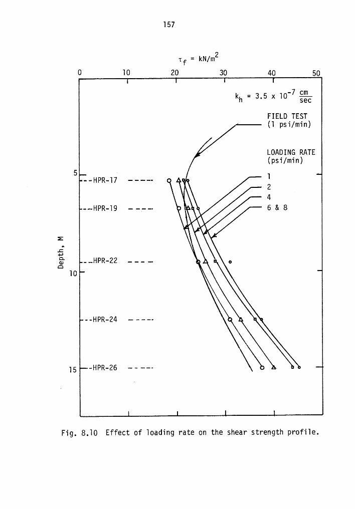
l57

Tf = kN/m20 TO 20 30 40 50

_ -7 cmkh — 3.5

XFIELD TEST(l psi/min)

LOADING RATE(psi/min)

5 · 1--HPR—l7 —-——- • ···· 24---HPR-l9 ——--· • · 6 8 8

2.é+>

·-—— —• „• A Q¤l0

--HPR-24 ————· * ^ ·

15 -HPR-26 ————· • ~ ·

Fig. 8.lO Effect of loading rate on the shear strength profile.

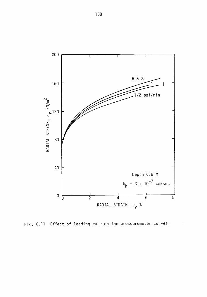
158

200

6 & 8160 4 1

1/2 psi/min€\lE\Z.>¢

,120O

MI·—V)

Q<ZM

40Depth 6.8 M

kh = 3 x10_7

cm/sec


Fig. 8.11 Effect of 1oading hate on the pressuremeter curves. ·

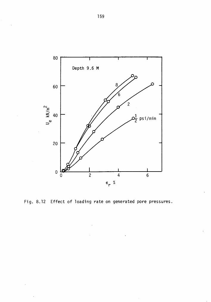
159

80

Depth 9.6 M••

60 8 °6

O

N

•• 2 .E

E? 40D 0

•20 •

••

l •

0 *4:0 2 4 6

er %

Fig. 8.12 Effect of 10ading rate on generated pore pressures.

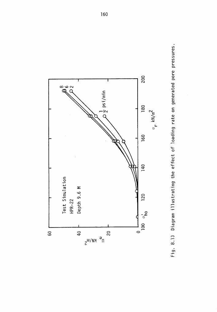
160

U)GJLI3U)U)CULQ.GJL

G OG Q.<\|

'UGkOC\I (U0) Q C 1;

•'1 L lE cuX C.,.. Q)U) C7Q. G

G C·-lm «— ALE o(Ü •

·

\ CDZ 4-*A6 fü

LLO U)

C•«—‘ G U

LO fü— (GQ Q •— O\_ r—·\ *4-

O_ 4-*

UGJZIil ÖIll C, Q)

e- CD.C

C 4-*O

4-* CFU Z ·•-·r- • 4-*3 RO 1 FUE · V C) L•v· O) C\1 4-*

C/) C\I •— U)(\1 .C 3

4-* I 4-) r-U) Df. CL •—Q) Q. Q) ·¤··I- I G O— -.: EI o ru

LO')G füO '•—r-- G

G G G GLO <' AI

U,l/ S 2N*1 {1 -Z ooO)•r-

LL.

l6l

for l psi/min. The finding, which is by no means a trivial one,

brings the Stanford pressuremeter tests within the general consensus

of the geotechnical engineering profession that the pressuremeter

yields a higher shear strength than that given by the vane shear test.

As evident from Fig. 8.ll, the rate of loading does not seem to

affect the initial slope, and hence the shear modulus, of the pressure-

meter curves. To precisely verify the fact, the pressuremeter curves

at different loading rates were fitted by cubic splines and the initial

slopes taken as twice the shear modulii. The results are shown in

Table 8.l. The difference in the values of G in the range of loading

rates, l to 6 psi/min, is insignificant. _(

_

8.4 EFFECT OF PERMEABILITY AND LOADING RATE

what is useful for the engineering practice is the Fig. 8.l4

where the test HPR—l9 is analyzed not only for varying permeability but

for different rate of loading as well. Corresponding to a chosen value

of permeability pressuremeter test simulations were made for different

loading rates. The dotted line corresponds to the undrained conditions.

It is seen in Fig. 8.l4 that for a permeability of lxlO-8 cm/sec, a

very slow loading rate shall be needed to cause any drainage and thus

the test may be considered undrained within the normal range of loading

rates in use today (i.e., l to 4 psi/min). On the other hand, for a

permeability of lxlO”5 cm/sec, it is not possible to run an undrained

test within any workable range of loading rates.

The conclusion must therefore be that under permissible range of

loading rates (l to 8 psi/min) undrained conditions can be achieved

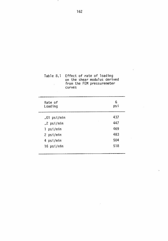
162

Tab1e 8.1 Effect of rate of 1oadingon the shear modu1us derivedfrom the FEM pressuremetercurves

Rate of GLoading psi .

.01 psi/min 437

.2 psi/min 4471 psi/min 4692 psi/min 4834 psi/min 504

A

16 psi/min 518

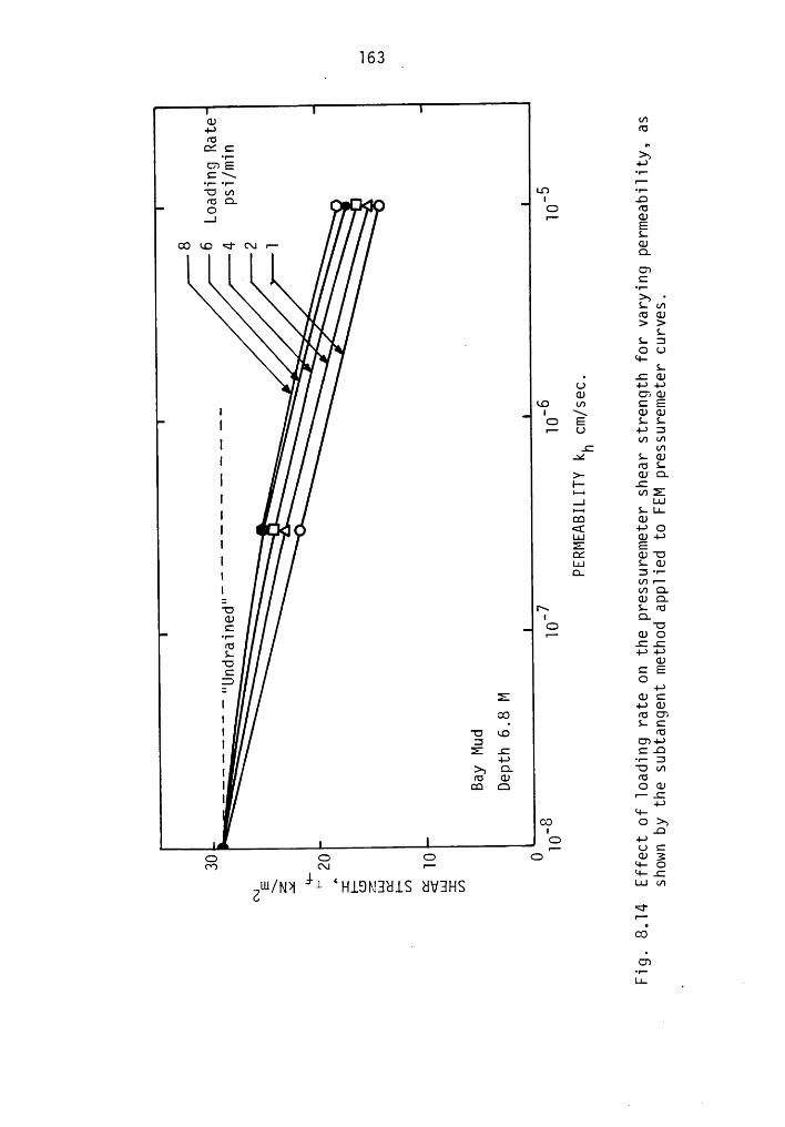
U'!IG FU0:: ,,

-1-maCi .I.-1--1-

I_

E8“‘ '·*

Q O .40 IG -2.J I., Q)

E

O.

_ C7C

-1->, „S.U‘!FGO)

I >>

'

S.I. . s.:

·

OUI. ‘·!-S.

I gwU 4-*4-*GJ CNG)

[ SO U} CEI \ GJCU

I G E s.s.•— U 4-*3I L mm

U!I x s.q;

¢‘US—I.C' 3 "EII'

ä ä"I Ct <u·¤

!.1.! S-C1)I O. Zw-

I(f)1—

= äßäE ·7 ;·¤F G ·¤; r— QJOL .C.C.¤ 4-*4-*g cg-

O

I -CDC

I OOpg-r¤ I

·U .6

‘·äI 3 G4->I

c.¤· 3

I >¤ Q- Em[ FU CU YU

CQ Q Qq)I

1-:4-*

O3I .Q

C> O O@2 Ü:

Q LZw/N>! L HiE)!.!E!E!.LS HVHHS '—·-*<^<I'1-

O

®

O7*|*L1.. I _

l64’

only in soils with permeabilities less than lxlO”8 cm/sec, and that

some drainage will necessarily occur if the permeability is higher

thanlxlO”8

cm/sec.

8.5 RECOMMENDED PROCEDURE FOR CONDUCTING PRESSUREMETER TESTS _

Based on the observations made during this investigation, a

guideline for conducting self-boring pressuremeter tests is set up in

consultation with Dr. Jean Benoit of the University of New Hampshire.

The major question in the test is the estimation of minimum loading

rate for which the test shall be nearly undrained. Therefore, it is

recommended that before embarking on a comprehensive testing program,

a set of two holding tests at different depths should be carried out

and the permeability of the stratum be assessed.

The finite element analysis may then be used to derive a plot

similar to Fig. 8.l4 whereby a suitable loading rate can be determined.

It may be mentioned that only a rough estimate of Cam Clay parameters

is needed to reach at acceptable results, and such an estimate can be

made on the basis of index properties of the soil alone. Wood and

wroth (l978) present useful correlations for this purpose.

In addition, it is suggested that the field testing program p

(awfully expensive, as it normally is) be supported on a daily basis _

by a finite element analysis. At a cost of less than l% of the field

expense, such an analysis may provide a useful insight into the test

data obtained.

·CHAPTER 9

SUMMARY AND CONCLUSIONS

9.l SUMMARY

This dissertation presents a study of the self-boring pressure-

meter test. This instrument has been recognized by the geotechnical

engineering profession for having a high potential for use in in-situ

testing of soils. However, the appeal of the test has been limited, in

part, because of several unanswered questions attached with the test.

Primarily these questions concern the unknown drainage conditions en-

countered in the test, and the effects of disturbance in the soil during

the insertion of the probe. This study investigates the question of

drainage during the pressuremeter test. The investigation involves the

following:

l. Implementation of a numerical finite element model, in-

corporating nonlinear soil behavior with capability of

couple consolidation, to simulate the phenomenon en-

countered in the pressuremeter test.

2. A laboratory test program to evaluate the soil constants

needed in the model._4

3. Calibration of the finite element model using a series of

field pressuremeter tests performed in San Francisco Bay

Mud.

4. Use of the finite element model for parameteric studies

concerning drainage and pore pressure dissipations in the

T65

T l66

pressuremeter test.~

. For the laboratory test program, five tubes of undisturbed soil

samples of San Francisco Bay Mud were imported from the Hamilton Air

Force Base Station in Navato, California, where the self-boring

pressuremeter tests were conducted. The tube samples were tested in

the laboratory by the author in order to determine the stress-strain

and consolidation characteristics of the Bay Mud. A special effort was

made to evaluate the horizontal flow characteristics of Bay Mud in the

laboratory by isotropic and oedometric consolidation tests. It is

found that isotropic consolidation leads in general to lower estimates

of the coefficient of consolidation than estimates produced by the

oedometer test on vertical specimen. The coefficient of consolidation

given by the oedometer tests on vertical specimen is found to be 2 to

3 times higher than the values given by oedometer tests on horizontal

specimen. ·

A finite element program, PEPCO (Johnston and Clough, l980) was _

chosen for the investigation. The program was modified to utilize it

for modeling the pressuremeter test.

9.2 CONCLUSIONS

The investigation asserts that the finite element method incorpo-

rating Biot's theory of consolidation and the concepts of critical

state soil mechanics is capable of modeling, to an acceptable accuracy,

the phenomenon encountered in the pressuremeter test in soft clays. It

presents for the first time a comparison between the finite element

results and the field pressuremeter test in soft clays.

l67

It is shown that through finite element simulation it is possible

to backfigure from the pressuremeter curves a segment of soil constants

if the remaining soil constants are known. The finite element modeling

can also help assess the quality of the test data obtained.

It is proven through axisymmetric analyses of pressuremeter tests

that the soil at the mid-height of the probe indeed deforms in a mode

of vertical plane strain, and that drainage, if any, takes places pre-

dominantly in the horizontal direction. Therefore, it is valid to

investigate the pressuremeter test utilizing a simple axisymmetric-

plane strain element. The finding is supported by comparisons between

the results of the axisymmetric and the axisymmetric—plane strain

analyses.

The study provides an understanding of drainage phenomena in the

pressuremeter test. It is found that the computed shear strength may

significantly deviate from its undrained value if partial drainage

occurs during the test but the pressuremeter data is analyzed assuming

the test to have been undrained. It is discovered that only when the

soil has a permeability of lxl0'8 cm/sec, or lower, it is possible to

run a perfectly undrained test. In soils with permeabilities higher

than lxl0-8 cm/sec, some drainage will necessarily occur during the

test for a feasible range of loading rates (l to 8 psi/min). For ’

permeabilities of the order of lxl0”5 cm/sec, undrained conditions

cannot be achieved for any practable range of loading rates in the

pressuremeter test.U

A comparison of the laboratory—determined values of the hori-

zontal coefficient of consolidation with those of the pressuremeter

l68

holding test provides a limited evidence for accepting the latter as a

promising partner in field investigation of soils. It is found that a

value of horizontal permeability, 5 times that of vertical permeability,

reported by Benoit (l983) from his holding tests, best simulates the

field pressuremeter tests.

Finally, it is shown that, by simulating the pressuremeter test

by a numerical model, it is possible to determine the required loading

rate at which the test should be conducted so the soil deforms under

nearly undrained condition. The proposed test procedure for conducting

the pressuremeter tests in the field is believed to be a step forward

in the process of standardizing the self-boring pressuremeter test.

Added understanding of the mechanics of the pressuremeter test and re-

finements provided by the proposed testing procedure will lead to

consistancy in the results, and therefore, will give the profession an

increased confidence in this novel testing device.

REFERENCES

Amar, S., Bague1in, F., Jezeque1, J. F. and Le Mahaute, A. (1975)."In Situ Shear Resistance of C1ays." Proc. ASCE Spec. Conf. onIn Situ Measurement of Soi1 Properties, Ra1eigh, Vo1. I, pp. 22-45. ·

Atkinson, J. H. and Bransby, P. L. (1978). The Mechanics of Soi1s:An Introduction to Critica1 State Soi1 Mechanics, McGraw-Hi11,London.

Bachus, R. C., C1ough, G. N., Sitar, N., Shafii—Rad, N., Crosby, J.,and Kabo1i, P. (1981). "Behavior of weak1y Cemented Soi1S1opes under Static and Seismic Loading Conditions, Vo1. II,"Report No. 52, The John A. B1ume Earthquake Engineering Center,Stanford University.

Bague1in, F., Jezeque1, J-F., LeMee, E., and Le Mehaute, A. (1972)."Expansion of Cy1indrica1 Probes in Cohesive Soi1s." Journa1 ofthe Soi1 Mechanics and Foundations Division, ASCE, Vo1. 98, No.SM11„ PD. 1129-1142.

Bague1in, F., Jezeque1, J. F., and Le Mehaute, A. (1974). "Se1f-Boring P1acement Method of Soi1 Characteristics Measurements."Proc. ASCE Spec. Conf. on Subsurface Exp1oration for UndergroundExcavation and Heavy Construction, Henniker, New Hampshire,pp. 312-332.

Bague1in, F., Jezeque1, J-F., Shie1ds, D. H. (1978). The Pressure-meter and Foundation Engineering. Trans Tech Pub1ications,C1austha1, Germany.

Banerjee, P. K. and Stipho, A. S. (1978). "Associated and Non-associated Constitutive Re1ations for Undrained Behavior ofIsotropic Soft C1ays." Internationa1 Journa1 for Numerica1 andAna1ytica1 Methods in Geomechanics, Vo1. 2, pp. 35-56.

Benoit, J. (1983). "Ana1ysis of Se1f—boring Pressuremeter Tests inSoft C1ay." Ph.D. Thesis, Stanford University.

Besse1ing, J. F. (1953). "A Theory of P1astic F1ow for AnisotropicHardening in P1astic Deformation of an Initia11y IsotropicMateria1." Nat. Aero. Res. Inst., Amsterdam, Report $-410.

Biot, M. A. (1941). "Genera1 Theory of Three-Dimensiona1 Conso1ida-tion." Journa1 of App1ied Physics, Vo1. 12, pp. 135-164.

169

170

Bishop, A. N. and Henke1, D. J. (1962). The Measurement of Soi1Properties in the Triaxia1 Test, 2nd Ed. Adward Arno1d, London.

Bishop, R. F., Hi11, R., and Mott, N. F. (1945). "The Theory ofIndentation and Hardness Tests." Proceedings of the Physica1Society, Vo1. 57, p. 47.

Bonaparte, R. and Mitche11, J. K. (1979). "The Properties of SanFrancisco Bay Mud at Hami1ton Air Force Base, Ca1ifornia."Department of Civi1 Engineering, University of Ca1ifornia,Berke1ey.

Booker, J. R. and Sma11, J. C. (1975). "An Investigation of theStabi1ity of Numerica1 So1utions of Biot's Equations ofConso1idation." Internationa1 Journa1 of So1ids and Structures,Vo1. 2, pp. 907-917.

Bur1and, J. B. (1971). "A Method of Estimating the Pore Pressuresand Disp1acements Beneath Embankments on Soft, Natura1 C1ayDeposits." Stress-Strain Behavior of Soi1s, Proc. RoscoeMemoria1 Symposium, Cambridge University.

Ca11adine, C. R. (1963). "The Yie1ding of C1ay." Geotechnique, Vo1.13, pp. 250-255.

Carter, J. P., Booker, J. R. and Sma11, J. C. (1979). "The Ana1ysisof Finite E1asto-P1astic Conso1idation." Internationa1 Journa1for Numerica1 and Ana1ytica1 Methods in Geomechanics, Vo1. 3,pp. 107-129.

Carter, J. P., Rando1ph, M. F. and wroth, C. P. (1979). "Stress andPore Pressure Changes in C1ay During and After the Expansion of aCy1indrica1 Cavity." Internationa1 Journa1 for Numerica1 andAna1ytica1 Methods in Geomechanics, Vo1. 3, pp. 305-322.

C1arke, B. G., Carter, J. P. and wroth, C. P. (1979). "In-SituDetermination of the Conso1idation Characteristics of SaturatedC1ays." Proceedings of the Seventh European Conference on Soi1Mechanics and Foundation Engineering, Brighton, Vo1, 2, pp. 207-213.

C1ough, G. W. and Benoit, J. (In Press). "Use of the Se1f-BoringPressuremeter in Soft C1ays." Chapter 5 in Deve1opments inGeotechnica1 Engineering, E1sevier Pub. Co.

C1ough, G. N. and Denby, G. M. (1980). "Se1f-Boring PressuremeterStudy on San Francisco Bay Mud." Journa1 of the Geotechnica1Engineering Division, ASCE, Vo1. 106, No. GT1, pp. 45-63.

171

C1ough, G. N. and Si1ver, M. L. (1983). "A Report of the workshopon Research Needs in Experimenta1 Soi1 Engineering." VirginiaPo1ytechnic Institute and State University, B1acksburg, Virginia.

Denby, G. M. (1978). "Se1f—Boring Pressuremeter Study of the SanFrancisco Bay Mud." Ph.D. Thesis, Stanford University,Ca1ifornia.

Denby, G. M. and C1ough, G. W. (1980). "Se1f—Boring PressuremeterTests in C1ay." Journa1 of the Geotechnica1 Engineering Division,ASCE, Vo1. 106, No. GT12, pp. 1369-1387.

Drucker, D. C., Gibson, R. E. and Henke1, D. J. (1957). "Soi1Mechanics and work-Hardening Theories of P1asticity." Trans.ASCE, Vo1. 122, pp. 338-346.

Drucker, D. C. and Pa1gen, L. (1981). "0n Stress—Strain Re1ationsSuitab1e for Cyc1ic and 0ther Loading." Journa1 of App1iedMechanics, ASME, Vo1. 48, pp. 479-485.

Duncan, J. M. (1965). "Effect of Anisotropy and Reorientation ofPrincipa1 Stresses on the Shear Strength of Saturated C1ays."Ph.D. Thesis, University of Ca1ifornia, Berke1ey.

Duncan, J. M. and Buchignani, A. L. (1976). "An Engineering Manua1for Sett1ement Studies." Department of Civi1 Engineering,University of Ca1ifornia, Berke1ey.

Duncan, J. M., Byrne, P., Wong, K. S. and Mabry, P. (1980). "Strength,Stress-Strain and Bu1k Modu1us Parameters for Finite E1ementAna1ysis of Stresses and Movements in Soi1 Masses." Report No.UCB/GT/80-01, University of Ca1ifornia, Berke1ey, 77 pages.

Duncan, J. M. and Chang, C. Y. (1970). "Non1inear Ana1ysis of StressStrain in Soi1s." Journa1 of the Soi1 Mechanics and FoundationEngineering Division, ASCE, Vo1. 96, No. SM5, pp. 1625-1653.

Duncan, J. M. and Seed, H. B. (1967). "Corrections for Strength TestData." Journa1 of the Soi1 Mechanics and Foundations Division,ASCE, Vo1. 93, pp. 121-137.

Gibson, R. E. and Anderson, W. F. (1961). "In—Situ Measurement ofSoi1 Properties with the Pressuremeter." Civi1 Engineering andPub1ic works Review, Vo1. 56, pp. 615-618.

Hartman, J. P. and Schmertmann, J. H. (1975). "Finite E1ement Studyof the E1astic Phase of Pressuremeter Tests." Proceedings ofthe Specia1ty Conference on the In-Situ Measurement of Soi1Properties, Ra1eigh, North Caro1ina, ASCE, Vo1. I, pp. 190-207.

172

Iwan, N. D. (1967). "0n a C1ass of Mode1s for the Yie1ding Behaviorof Continuous and Composite Systems." J. App1. Mech., Vo1. 34,No. 3, PP. 612-617.

Jain, S. K. (1979). "Some Fundamenta1 Aspects of the Norma1ity Ru1eand Their Ro1e in Deriving Constitutive Laws of Soi1s." M.S.Thesis, Virginia Po1ytechnic Institute and State University,B1acksburg, Virginia.

Johnston, P. R. and C1ough, G. W. (1983). "Deve1opment of a DesignTechno1ogy for Ground Support for Tunne1s in Soi1 —— Vo1. I:Time Dependent Response Due to Conso1idation in C1ays."Stanford University Report to the U.S. Department of Transporta-tion, Rep. No. DOT-TSC—UMTA-82-54, 1.

Ladanyi, B. (1972). "In-Situ Determination of Undrained Stress StrainBehavior of Sensitive C1ays with the Pressuremeter." CanadianGeotechnica1 Journa1, Vo1. 9, pp. 313-319. _

Ladd, C. C., Foott, R., Ishihara, K., Sch1osser, F. and Pou1os, H. G.(1977). "Stress - Deformation and Strength Characteristics."Proceedings of the Ninth Internationa1 Conference on Soi1Mechanics and Foundation Design, Tokyo, Vo1. 2, pp. 421-494.

Ladd, C. C. and Foott, R. (1974). "New Design Procedure forStabi1ity of Soft C1ays." Journa1 of the Geotechnica1 EngineeringDivision, ASCE, Vo1. 100, GT7, pp. 763-786.

Ladd, C, C., Germaine, J., Ba1igh, M. and Lacasse, S. (1980)."Eva1uation of Se1f-Boring Pressuremeter Tests in Boston B1ueC1ay." Federai Highway Administration Interim Report, No.FHNA/RD—80/052.

Lade, P. V. and Duncan, J. M. (1973). "Cubica1 Triaxia1 Tests onCohesion1ess Soi1." Journa1 of the Soi1 Mechanics and Founda-tions Division, ASCE, Vo1. 99, pp. 793-812.

Menard, L. F. (1956). "An Apparatus for Measuring the Strength ofSoi1s in P1ace." M.S. Thesis, University of I11inois.

Mitche11, J. K. and Lunne, T. (1977). Unpub1ished fie1d vane shear _tests reported in Bonaparte and Mitche11 (1979).

Mroz, Z. (1967). "0n the Description of Anisotropic work-Hardening."J. Mech. Phys. So1ids, Vo1. 15, pp. 163-175.

Mr¤Z»Z-(1973,)-University of water1oo Press.

173

Pa1mer, A. C. (1972). “Undrained P1ane-Strain Expansion of aCy1indrica1 Cavity in C1ay: A Simp1e Interpretation of thePressuremeter Test." Geotechnique, Vo1. 22, No. 3, pp. 451-457.

Prevost, J. H. and Hoeg, K. (1975). "Ana1ysis of Pressuremeter inStrain-Softening Soi1." Journa1 of the Geotechnica1 EngineeringDivision, ASCE, Vo1. 101, No. GT 8, pp. 717-731.

Prevost, J. H. (1977). "Mathematica1 Mode11ing of Monotonic andCyc1ic Undrained C1ay Behavior." Int. J. Num. Ana1. Meth.Geomech., Vo1. 1, pp. 195-216.

Rando1ph, M. F. and wroth, C. P. (1979). "An Ana1ytica1 So1ution forthe Conso1idation Around a Driven Pi1e." Internationa1 Journa1for Numerica1 and Ana1ytica1 Methods in Geomechanics, Vo1. 3,pp. 217-229.

Roscoe, K. H. and Bur1and, J. B. (1968). "Dn the Genera1ized Stress-Strain Behavior of 'wet' C1ay." Engineering P1asticity,Cambridge University Press, pp. 535-609.

Roscoe, K. H. and Poorooshash, H. B. (1963). "A Theoretica1 andExperimenta1 Study of Strains in Triaxia1 Compression Tests onNorma11y Conso1idated C1ays." Geotechnique, Vo1. 13, pp. 12-38.

Roscoe, K. H. and Schofie1d, A. N. (1963). "Mechanica1 Behavior ofan Idea1ized wet C1ay." Proc. European Conference in Soi1Mechanics, wiesbaden, Vo1. 1, pp. 47-54.

Roscoe, K. H., Schofie1d, A. N. and Thurairajah. (1963). "Yie1dingof Soi1s in States wetter than Critica1." Geotechnique, Vo1. 13,pp. 211-240.

Roscoe, K. H., Schofie1d, A. N. and Nroth, C. P. (1958). "Dn theYie1ding of Soi1s." Geotechnique, Vo1. 8, pp. 22-53.

Sandhu, R. S. and wi1son, E. L. (1969). "Finite-E1ement Ana1ysis ofSeepage in E1astic Media." Journa1 of the Soi1 Mechanics andFoundations Division, ASCE, Vo1. 95, pp. 285-312.

Schiffmann, R. L., Chen, A. T. F. and Jordan, J. C. (1969). "AnAna1ysis of Conso1idation Theories." Journa1 of the Soi1Mechanics and Foundations Division, ASCE, Vo1. 95, pp. 285-312.

Schofie1d, A. N. and Nroth, C. P. (1968). Critica1 State Soi1Mechanics, McGraw-Hi11, London.

Sinram, A. (1984). "Cubica1 Shear Box Tests Designed to Simu1atePressuremeter Loadings." Thesis in Progress for the Partia1Fu1fi11ment of the Engineer Degree, Stanford University.

l74

Small, J. C., Booker, J. R. and Davis, E. H. (l976). "Elasto-Plastic Consolidation of Soil." International Journal of Solidsand Structures, Vol. l2, pp. 43l-448. I

Szavits-Nossan, A. (l982). "A Kinetmatic Model for Sands." Proc.Int. Conf. Constitutive Laws for Engineering Materials. Tucson,Arizona, pp. 285-288.

Tavenas, F. A., Blanchette, G., Leroveil, S., Roy, M. and LaRochelle, P.(l975). "Difficulties in the In-Situ Determination of KO in SoftDensitive Clays." Proceedings of the Specialty Conference on theIn-Situ Measurement of Soil Properties, Raleigh, North Carolina,ASCE, Vol. l, pp. 450-476.

Taylor, G. I. and Ouinney, H. (l932). "The Plastic Distortion ofMetals." Phil. Trans. Royal Society, Series A, Vol. 230, pp. 323-363.

Terzaghi, K. and Peck, R. B. (l967). Soil Mechanics in EngineeringPractice, Wiley, N.Y.

Tringale, P. T. (l978). Unpublished field vane shear tests, reportedin Bonaparte and Mitchell (1979).

White, G. N. (l95l). "Application of the Theory of Perfectly PlasticSolids to Stress Analysis of Stress Hardening Solids." Div. ofAppl. Maths., Brown University, T.R. 5l.

Wood, D. M. and Wroth, C. P. (l977). "Some Laboratory ExperimentsRelated to the Results of Pressuremeter Tests." Geotechnique,Vol. 27, No. 2, pp. l8l-20l.

Wroth, C. P. (l97l). "Some Aspects of the Elastic Behavior of Over-consolidated Clay." Stress-Strain Behavior of Soils, Proc.Roscoe Memorial Symposium, Cambridge University.

Wroth, C. P. (l975). "In—Situ Measurement of Initial Stresses andDeformation Characteristics." Proceedings of the SpecialtyConference on the In-Situ Measurement of Soil Properties,Raleigh, North Carolina, ASCE, Vol. 2, pp. l8l—230.

Wroth, C. P. and Hughes, J. M. O. (l973). "Undrained Plane StrainExpansion of a Cylindrical Cavity in Clay -- A Simple Interpre-tation of the Pressuremeter Test." Discussion, Geotechnique,Vol. 23, No. 2, pp. 284-287.

Wroth, C. P. and Hughes, J. M. O. (l972). "An Instrument for theIn-Situ Measurement of the Properties of Soft Clays." ReportCUED/C-SOILS TR l3, University of Cambridge, England.

175

wroth, C. P. and Hughes, J. M. O. (1973). "An Instrument for theIn-Situ Measurement of Properties of Soft C1ays." Proceedingsof the Eighth Internationa1 Conference on Soi1 Mechanics andFoundation Engineering, Moscow, U.S.S.R., Vo1. 1.2, pp. 487-494.

wroth, C. P. and Hughes, J. M. O. (1974). "Deve1opment of a Specia1Instrument for the In-Situ Measurement of the Strength andStiffness of Soi1s." Proc. ASCE Spec. Conf. on SubsurfaceExp1oration for Underground Excavation and Heavy Construction,Henniker, New Hampshire, pp. 295-311.

wroth, C. P. and wood, D. M. (1978). "The Corre1ation of IndexProperties with Some Basic Engineering Properties of Soi1s."Canadian Geotechnica1 Journa1, Vo1. 15, No. 2, pp. 137-145.

Zienkiewicz, O. C. (1977). The Finite E1ement Method, McGraw-Hi11,3rd Edition.

Zienkiewicz, O. C., Nayak, G. C. and Owen, D. R. J. (1972). "Compositeand Over1ay Mode1s in Numerica1 Ana1ysis of E1asto—P1asticContinua." Foundations of P1asticity. Ed. A. Sawczuk.Noordhoff Press, pp. 107-122.

Zienkiewicz, O. C., Norris, V. and Nay1or, D. J. (1978). "P1asticityand Viscop1asticity in Soi1-Mechanics with Specia1 Reference toCyc1ic Loading Prob1ems." Proc. Int. Conf. Finite E1ements inNon1inear So1ids and Structura1 Mechanics, Gei1o, Norway, pp.455-485.

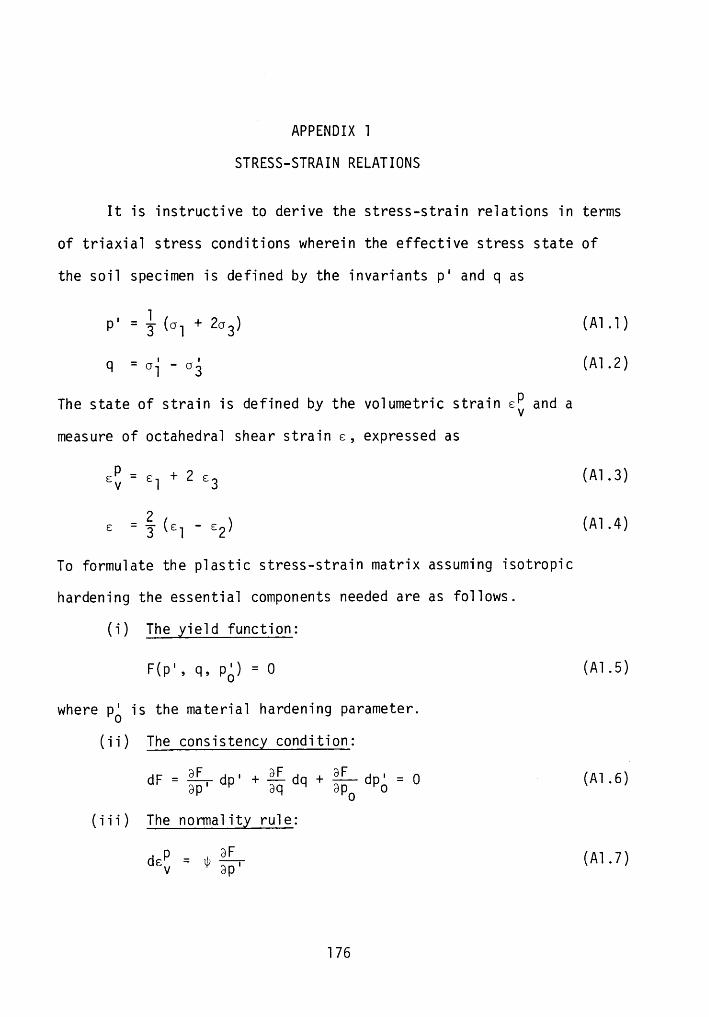
TAPPENDIX 1

STRESS-STRAIN RELATIONS

It is instructive to derive the stress-strain re1ations in terms

of triaxia1 stress conditions wherein the effective stress state of

the soi1 specimen is defined by the invariants p' and q as|_.l

p — §—(6] + 263) (A1.1)

q = Gi - Gé (A1.2)

The state of strain is defined by the vo1umetric strain 65 and a

measure of octahedra1 shear strain 6, expressed as

6p=6 +26 (A1.3)v 1 3

=?-(6 -6) (1-11.4)E 2 1 2To formu1ate the p1astic stress-strain matrix assuming isotropic

hardening the essentia1 components needed are as fo11ows.

(i) The yie1d function:

F<p', <1„ pg) = 0 (A1-5)where pg is the materia1 hardening parameter.

(ii) The consistency condition:

zi · Qi E. ·z2

dF Sp, dp + gq dq + gpc dpo 0 (A1.6)

(iii) The norma1ity ru1e:

P z .äE. A1 7däv176

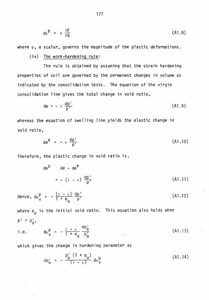
l77

p -E5de— w öq (A1.6)

where w, a scalar, governs the magnitude of the plastic deformations.

(iv) The work-hardening rule:

The rule is obtained by assuming that the strain hardening

properties of soil are governed by the permanent changes in volume as

indicated by the consolidation tests. The equation of the virgin

consolidation line gives the total change in void ratio,

de = — A ägl (Al.9)

whereas the equation of swelling line yields the elastic change in

void ratio,

dee = - K gg; (Al.l0)

Therefore, the plastic change in void ratio is,

dep de — dee

= - (A - K)

(A — ·<)QTLLHence,dg?] — ··

p,whereeo is the initial void ratio. This equation also holds when

p' = pg, I- dp'i.e.v O PO ·

which gives the change in hardening parameter as

dp, _ _ PQ, (‘* eo) dgp (Al.l4)

0_

(A - •<) V

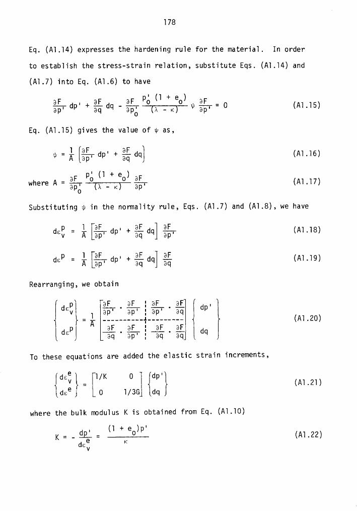
l78

Eq. (Al.l4) expresses the hardening rule for the material. In order

to establish the stress-strain relation, substitute Eqs. (Al.l4) and

(Al.7) into Eq. (Al.6) to have

' (l + e )0F . aF aF po 0 aF _

Eq. (Al.l5) gives the value of 0 as,

-i Qi:. · Qi:.0 —A [Sp, dp + öq dq} (Al.]6)

' (l + e )_ pr po 0 g_where A — 3p« (A:|·:l7)

Substituting 0 in the normality rule, Eqs. (Al.7) and (Al.8), we have

p : i. QE.. • QE. äE..dev A [ap, dp + Sq dq] Sp, (Al.l8)

p = i. ÄE.. • EE. EE.de A [ap, dp + öq dq] Bq (Al.l9)

Rearranging, we obtain

P Qi. . i I QL . E ·ddv 1 pp' pp' :G¤¤' SG dp2Z Z. ——__——————l———————¢—

dp ^Qi,p;E..ps.s»i d(Apo)

B SG pp' : GG pq d

To these equations are added the elastic strain increments,

B a B 1/k 0 dp·pv = (Al.2l)aeB 0 1/26 aqwhere the bulk modulus K is obtained from Eq. (Al.l0)

„ (l + G) ',2.-9);.. ...Q.p. (Al.22)dee K

V

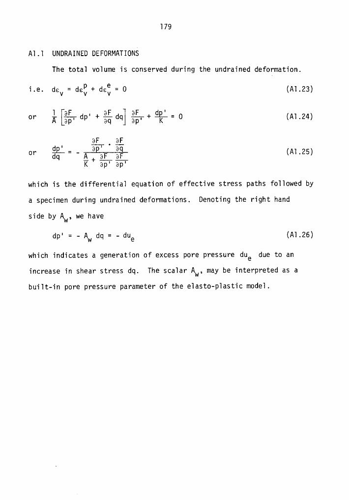
l79

Al.l UNDRAINED DEFORMATIONSThe total volume is conserved during the undrained deformation.

l.€. deV=de5+de$=O (ALZ3)

lL · L L Qi;-or A [Ap, dp + AQ dgl Ap, + K— 0 (Al.24)

L.3LQp;.-..e@'...¤s1.or dq A-+ AE- AE- (Al.25)K ap' ap'

which is the differential equation of effective stress paths followed by

a specimen during undrained deformations. Denoting the right hand

side by Aw, we have

dp' = - AW dq = - due (Al.26)

which indicates a generation of excess pore pressure due due to an

increase in shear stress dq. The scalar Aw, may be interpreted as a

built-in pore pressure parameter of the elasto—plastic model.

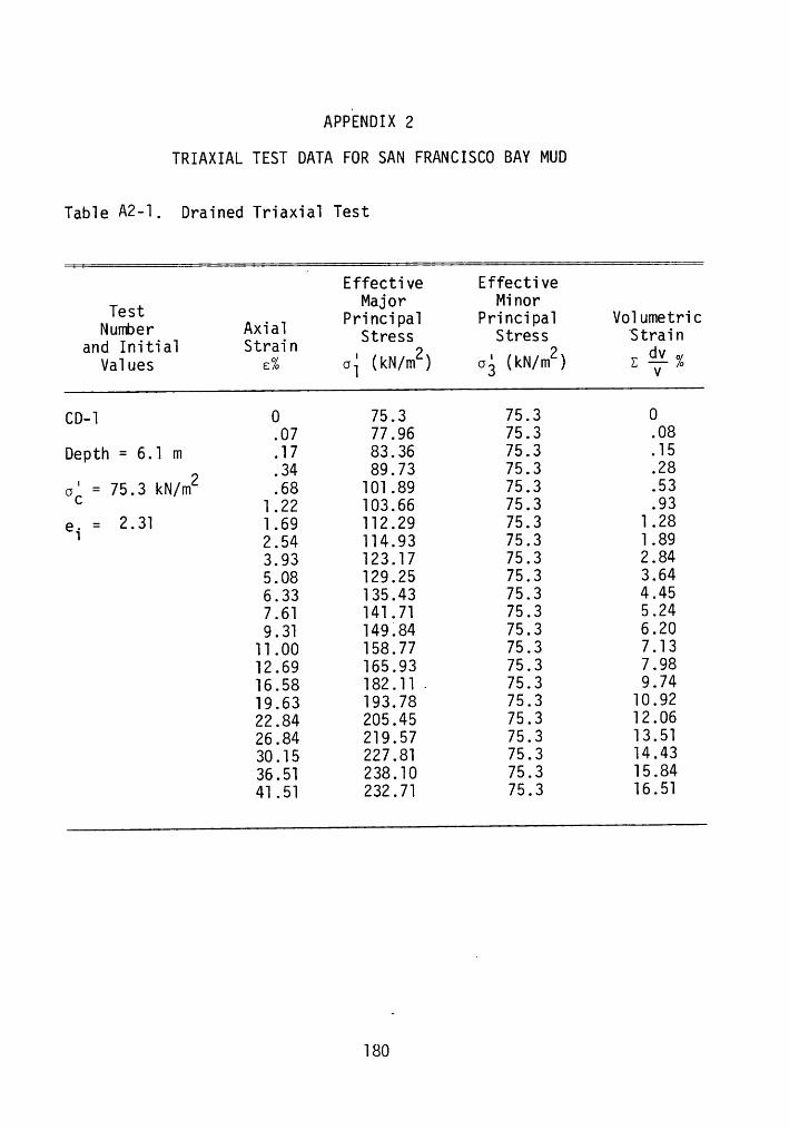
APPENDIX 2

TRIAXIAL TEST DATA FOR SAN FRANCISC0 BAY MUD

Table A2-]. Drained Triaxial Test

Effective EffectiveTest Mader Mine? .

Number Axiai Prgncipal Principal Vqlumetricand Initiai Strain ress Stress Strain

veiues e% ci (kN/mz) og (kN/mz)

zCD-]0 75.3 75.3 0.07 77.96 75.3 .08

Depth = 6.] m .]7 83.36 75.3 .]52 .34 89.73 75.3 .28

on = 75.3 kN/m .68 ]0].89 75.3 .53].22 ]03.66 75.3 .93

ei = 2.3] ].69 ]]2.29 75.3 ].282.54 ]]4.93 75.3 ].893.93 ]23.]7 75.3 2.845.08 ]29.25 75.3 3.646.33 ]35.43 75.3 4.457.6] ]4].7] 75.3 5.249.3] ]49.84 75.3 6.20

]].00 ]58.77 75.3 7.]3]2.69 ]65.93 75.3 7.98]6.58 ]82.]] . 75.3 9.74]9.63 ]93.78 75.3 ]0.9222.84 205.45 75.3 ]2.0626.84 2]9.57 75.3 ]3.5]30.]5 227.8] 75.3 ]4.4336.5] 238.]0 75.3 ]5.844].5] 232.7] 75.3 ]6.5]

]80

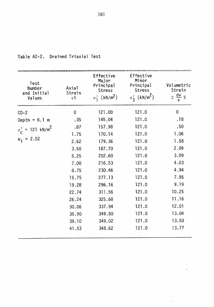
181

Tab1e A2—2. Drained Triaxia1 Test

Effective EffectiveTest . Pr?ää?ga1 Pr?62?ga1 V010metric

Qälggn Stress Stressz StäainVa1ues 6% ci (kN/mz) oä (kN/m ) Z T} %

CD-2 0 121.00 121.0 0Depth = 6.1 m .35 145.04 121.0 .18

O; = 12] kN/m2 .87 157.98 121.0 .501.75 170.14 121.0 1.06

ei = 2°02 2.62 179.36 121.0 1.583.50 187.70 121.0 2.095.25 202.60 121.0 3.097.00 216.53 121.0 4.038.75 230.46 121.0 4.94

15.75 277.13 121.0 7.9519.28 296.16 121.0 9.1922.74 311.56 121.0 10.2526.24 325.68 121.0 11.1630.06 337.94 121.0 12.0135.90 349.80 121.0 13.0439.10 349.02 121.0 13.5041.53 . 348.62 121.0 13.77

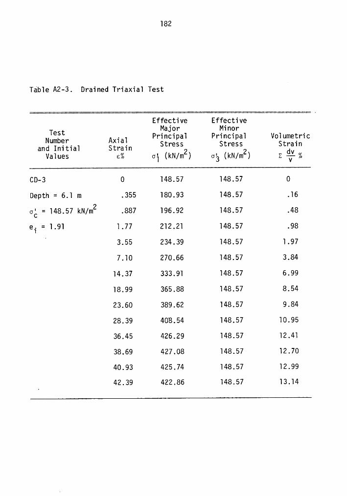
l82Table A2-3. Drained Triaxial TestEffective Effective

h

Näääär Axial PrTää?;al PrTlE$;al Volumetricand Initial Strain Stressz Stressz Stggin

Values 6% ci (kN/m ) dä (kN/m ) Z j7—%

CD-3 0 l48.57 l48.57 0

Depth = 6.l m .355 l80.93 l48.57 .l6

oé = l48.57 kN/mz .887 l96.92 l48.57 .48

ei = l.9l l.77 2l2.2l l48.57 .987 3.55 234.39 l48.57 l.97

7.l0 270.66 l48.57 3.84

l4.37 333.9l l48.57 6.99

l8.99 365.88 l48.57 8.54

23.60 389.62 l48.57 9.84

28.39 408.54 l48.57 l0.95

36.45 426.29 l48.57 l2.4l

38.69 427.08 l48.57 l2.70

40.93 425.74 l48.57 l2.9942.39 422.86 l48.57 l3.l4

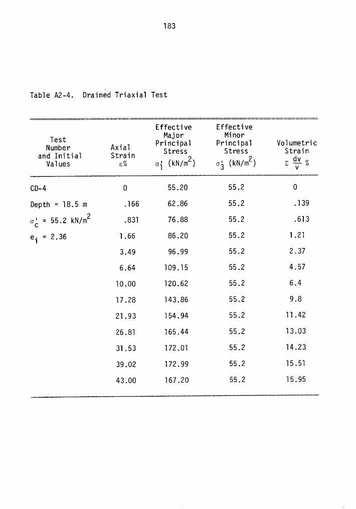
l83

Table A2-4. Drained Triaxial Test

Effective EffectiveTest Maier met

and Initial Strain- 2 2 dvValues 6% 6i (kN/m ) ¤ä (kN/m ) 2*TT %

CD—4 0 55.20 55.2 0

Depth = l8.5 m .l66 62.86 55.2 .l39

eé = 55.2 kN/m2 .83l 76.88 55.2 .6l3

ei = 2.36 l.66 86.20 55.2 l.2l3.49 96.99 55.2 2.37

6.64 l09.l5 55.2 4.57

l0.00 l20.62 55.2 6.4

l7.28 l43.86 55.2 9.8

2l.93 l54.94 55.2 ll.42

26.8l l65.44 55.2 l3.03

3l.53 l72.0l 55.2 l4.23

39.02 l72.99 55.2 l5.5l

43.00 l67.20 55.2 l5.95

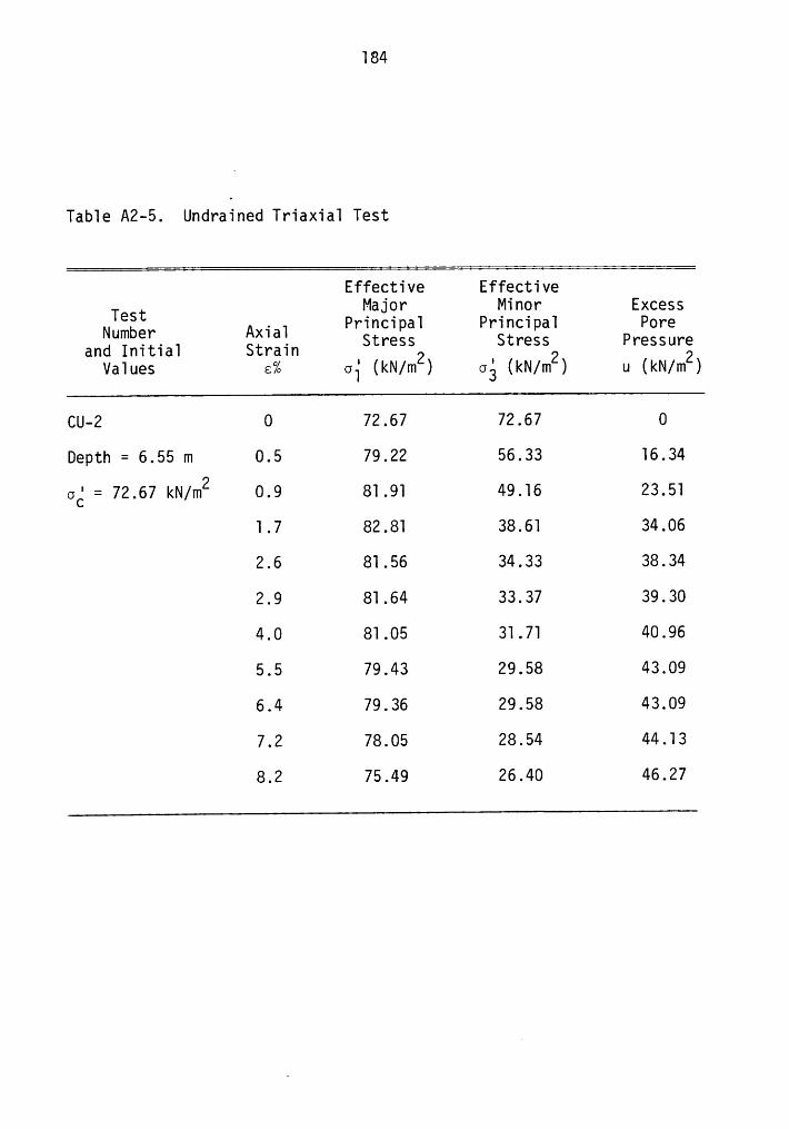
]84

Table A2-5. Undrained Triaxial Test

Effective EffectiveTest Major Minor Excess

. Principal Principal PoreNumber Axialand Initial Stnain Stressz Stressz Pressur;Values 6% oi (kN/m ) oé (kN/m ) u (kN/m )

CU-2 0 72.67 72.67 0

Depth = 6.55 m 0.5 79.22 56.33 ]6.34

og = 72.67 kN/m2 0.9 8].9] 49.]6 23.5]

].7 82.8] 38.6] 34.06

2.6 8].56 34.33 38.34

2.9 8].64 33.37 39.30

4.0 8].05 3].7] 40.96

5.5 79.43 29.58 43.09

6.4 79.36 29.58 43.09

7.2 78.05 28.54 44.]3

8.2 75.49 26.40 46.27

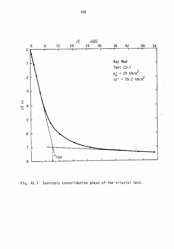
185

/t Vmin0 6 12 18 24 30 36 42 48 54

0

14 1

Bay MudTest CD-T

· pg = 20 kN/m22 .- 2Ap - 55.2 kN/m _

3

uu>¢1<¤ T

5

2 6

. 7 1 •It'100

8

Fig. A2.1 Isotropic c0ns01idati0n phase of the triaxia1 test. ‘

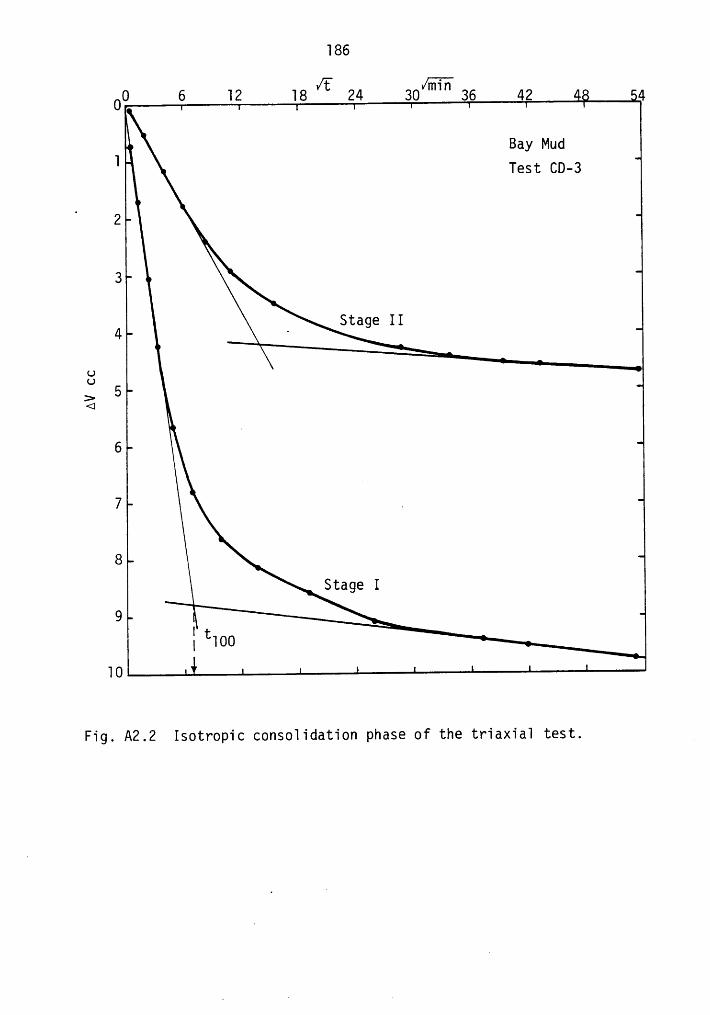
186

00 6 12 18 t 24 30 "“" 36 42 ·: 4

Ä” Bay Mud1 Test cp-6

_2

3

Stage II4

ou=_ 6<1 1 „

6

7 .

8Stage I

9

10

Fig. A2.2 Isotropic c0nso1idation phase of the triaxia1 test. p

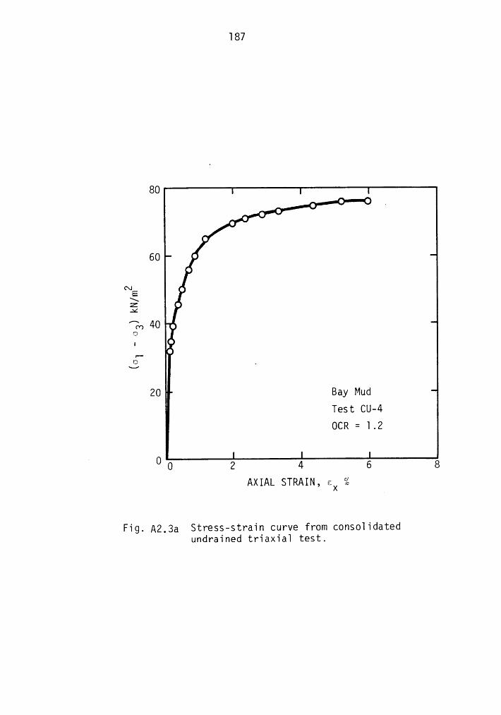
187

80• • • _.•°

•

60 •O

(XIE •\z •A6

0

' !LOJ3 I -

20I

Bay Mud* Test CU-4OCR = 1.2

Oo 2 4 6 6AXIAL STRAIN, ex %

Fig. A2,3a Stress-strain curve from conso1idatedundrained triaxia1 test.

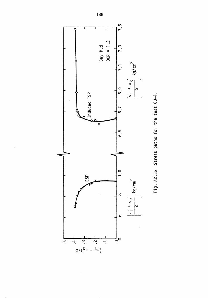
LO‘ 5

(\|'O r- C')3 •Z u r\>5 DSfü O

C\1P- E• U5 \U)

.¥

OOC')O

C7 + C\|

° Q. RO r- ·tf) O <i'IT. \—O—../ I

OU L)GJU 5 4-J

Q 3 ° U)• 'O CO GJO

·

|—|

·••4-*

LLO O• Q-LO

U).C4-*CU

· O.U')U')CUL

4-*V)

O .O• O")[7 O

NEU •

O')U) •¤—

..¥ LL

' ri-5·C\lO+ Gl—•—

OLo OO.;

OLO <!' C') C\.l r— O

lo)

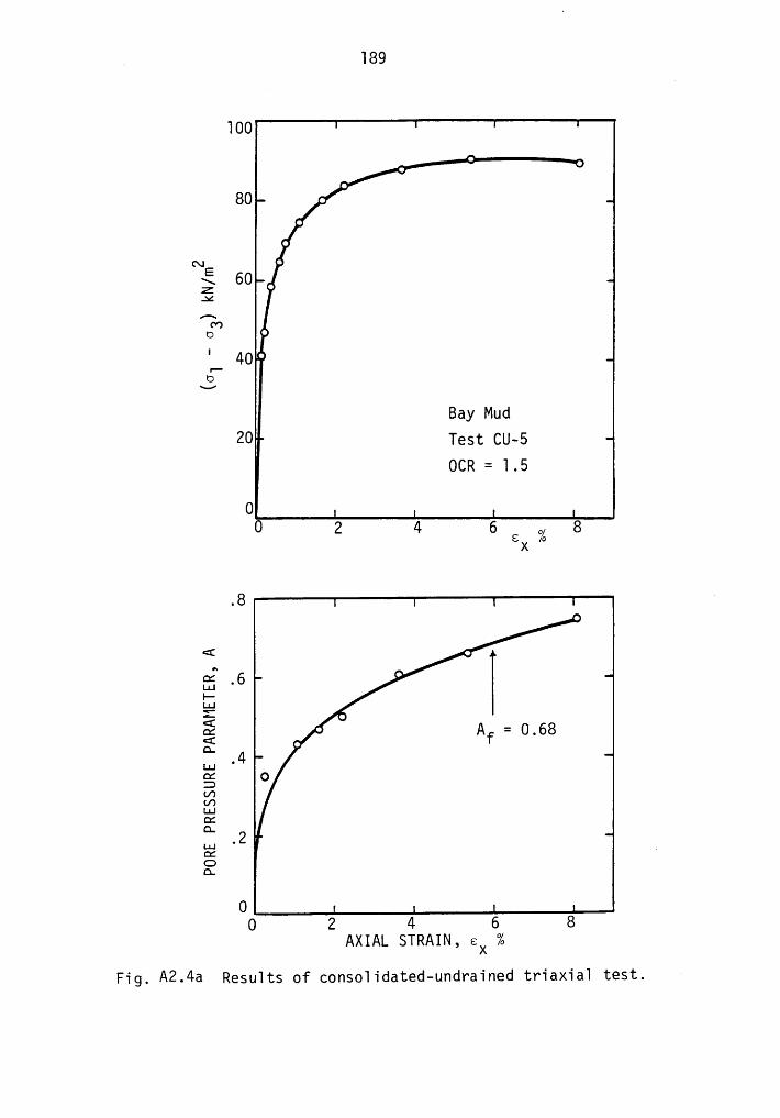
. 189

100

80 .°

ax1E •\ ÖÜ •E’?h¤ I

' 405Bay Mud

ZOI Test CU-54 OCR = 1.5

0Ü 2 4 6 0 86 AX

.8 ·

< O5;.6 • l1-ä!< Igg • • Af = 0.68¤.U; .4gf OmEä

.o¤.

00 2 4 6 8

AXIAL STRAIN, 6X %

Fig. A2.4a Resu1ts of cons01idated-undrained triaxia1 test.

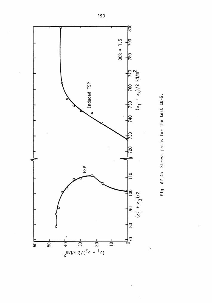
·GG••

LO¥•

II{IG3

. Gt\INE*2( Q-L/> GC\|}* SN

INU 00GJ ¤ ·

( U LnS ¤+ éq•-—• NO 4-)

<¤ $N CD‘ .C49

LS EN‘ anEG ¢'¤ü Q.

- cnU)CUJ L49U)

D• q-•O '__ •

t\l• <[• •• G U')

ON ·•··r-N U-/'\

-00O

¢ G+ON

'|*'

° o\-/

• .

EG G G G G G GLO LO ¢' (Y) C\.| r—

sn ‘Zw/Mx 2/( ¤ — ¤)

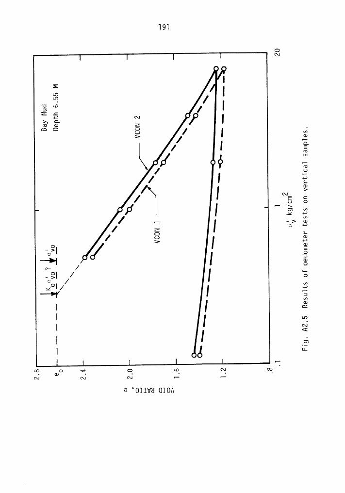
T9]

C\|

Z ILGC\I

IJ! I g/11

äI! I F E ::21/ ÜI1J 1 1;

A. 1 f-§’I / I 001

I $3I I SE1 I ·1 (I E

oo 0 <1- 0RQA;w A; A A —6 ‘011va 010A

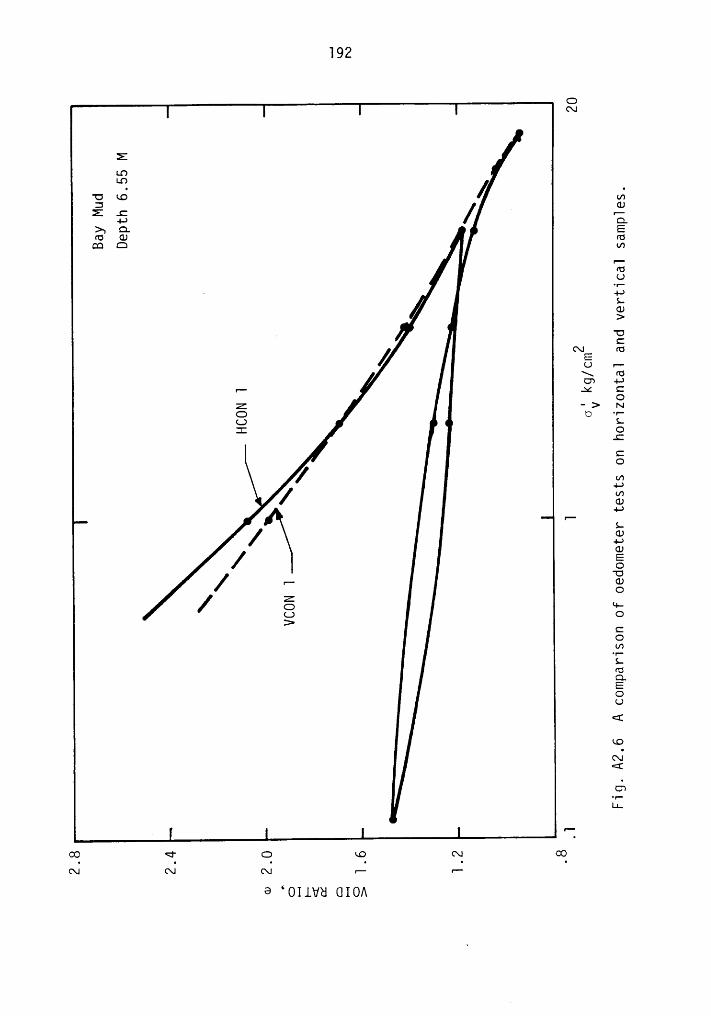
192

©C\|

ZLO“° /'U LO an

3 GJE .C / v—4-* Q

>, Q. Efü CU fü

CQ 2 chIZ

füU'|*

· 4-*LGJ>

. 'UC

C\I fü/ EL) r-

VÖC7 44r—· X C

OZ -> NO O ·¤··;_> LI O

£CO

/ ·¤44/ "’C1)44

IZ

LG)/ +—>CU/ EO

'Ur-· CDO

Z/ G “—LJ O> C

OU7°!*LfüQEOU

<E

RO<\I<K

C7'|*

LL

fi

GO <r Q ao N GOQ1 C\] C\| r— V"

69 OLLVH (110/\

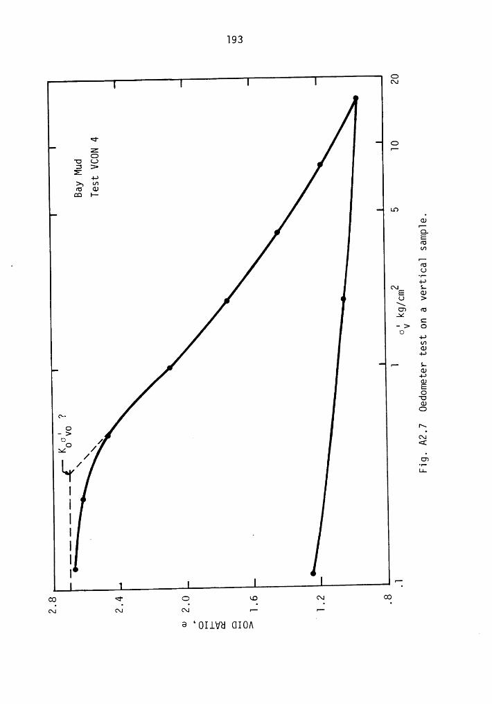
193

®C\|

Q- ®Z IT@

'U L.)I3 >Z

4-*>, Lnfü GJ

CO I-

LOGJ•—QEfüU7

v-. _r¤

U·«—4-*C\| L

E GJU >\U'! füat

C—> OO

4-*L/7GJ4-*

r- LGJ

4-*GJEO'UGJCD

qu.

O I\-> °C\1

>.4 / _/ U7/ ·•··L1.

I «——

oo <1- 0 no N GQQ; (\| C\1 r—

r····

G ‘011vu 0101

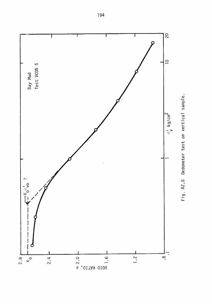
194

ON

CDLO |"

E'U LJ3 >E 4-*A anr¤ GJ

CQ 1-

¤3E-EFUU7

C\] IlE ¢¤U UA ·v··U3 4-*.>c LGJ-> >O

CU4-*anGJ4-*L

_ GJEO‘UGJO

/c~-2/ N

¤ / <G .G'3hy K

oo c Q- U ¤Q <\{ O?Ni ‘“ N N - -9 °OI.LVH CIIO/\

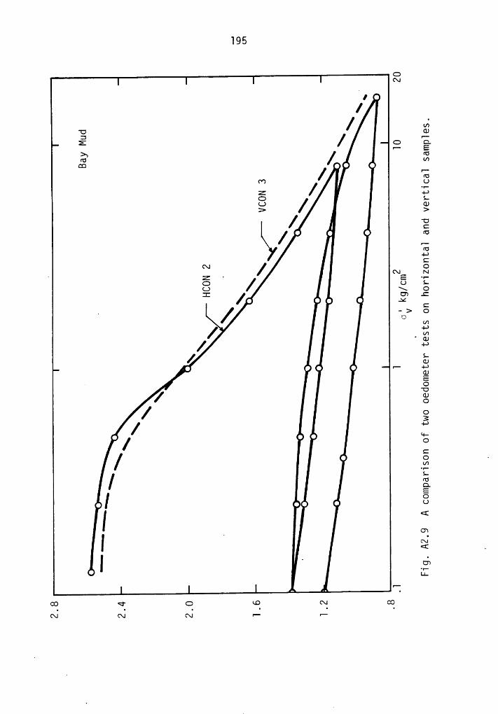
195

Ccx:ul •

Uf"

2* / 3¤3 •0 0

f'*

Z / u:CJ LS / S/ 1 2

/ • 0 0 asI3

N_Z _ mE NO / U EU \ OI / ¤¤ .:• 0 • 0 ac

. -> g0 3/ .=~[ S

/ 2.-0 00 0 ¤— +—*

S9I ES

f cuO

/ ¤3[ -1->#1-

!• •

Oc• 0 -mE’ rc9-

I 6• •• • U

I <1:_ cw

AI1 <E .

| 1 S' E

OO <r CJ no cu coC\J C\.I (\| •·— •—

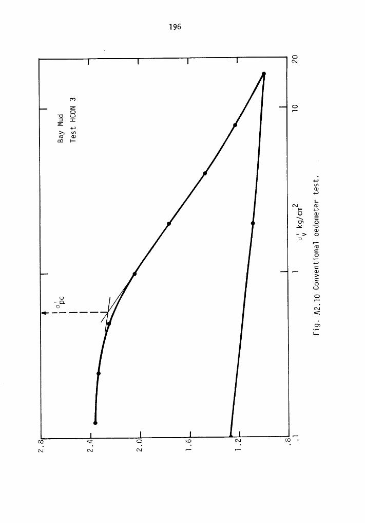
GC\l

O")

2°UC.)

3 IE -I-J>5 (/7fü CD

CQ }—

4-*L/7GJ4-}

LÄI GJE -•->

L) CUÄ EU') OAd 'U

GJ·> OO •—

füCO·r—

+-7Cr— GJ>COL)G-ä_ ""I

O cx.:·,,.._..—„L„.L• {

·•—L1.

e-co <r 0 no Q Q ·C\_| (\] (M r- r—·

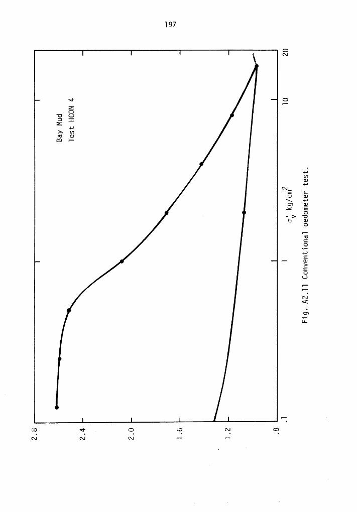
C\.l

<f Or-

ZO

°ULJ3]:Z -4-)>~,L/7füGJ@l—

4-*L/7GJ4-*C\|E L

U GJO7CUx E

O‘ ·>UO G)

Or-füCO

C•— GJ>COL)IT

I""

AI<E

OWLI.

OO <I'_ O ROC\1C\1C\I (\] P- •··—

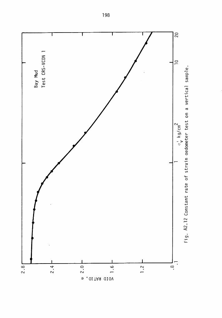
OC\|

r-ZOL.) O> IT

I•

V) G.)'U1 •—SO C}.Z E

4-* fü>,m anfüü)ml- ·—

fü'

'|*

4-*LG)>füCO4-*

CXI U)E CUU4-*EO')LA6 GJ

4-*->CU0 E

O'OCUOC

1- -1-füL

4-*U)

*4-OCU4-*füL

4-*Cfü4-*U)COLJC\|IO

Cl<E

U)'f*L;

IT

OO <‘ G LO (XI OOC\l (XI (XI IO IO

c9 OILVHGIOA

APPENDIX 3

A NOTE ON MULTI—SURFACE HARDENING MODELS*

Recent years have seen an increasing activity in the application

of multi-surface hardening models. while elegant formulations have

been made, there appears to be a blurring of the distinctions between

two basic approaches to formulating such models. It is the objective

of this note to bring out differences and similarities between the two

approaches. An attempt is made here to show that, while these

approaches employ the common feature of incorporating a set of nested

yield surfaces to extend the classical theory of plasticity, they dif-

fer in methametical formulations and originate from different physical

conceptions.

The first approach is that of composite structure formulations.

In this category are the white (l95l) and Besseling (l953) parallel

model, and Iwan's (l967) series model. The second approach is that of

integrated hardening variables model (Mroz, l967). In what follows,

we first give a brief description of each of these models and then out-

line essential differences between them.

*This note was prepared in association with Professor Z. Mroz whilehe served as a visiting professor in the Department of Civil Engineer-ing, during winter, l984. His assistance is gratefully acknowledged.

l99E

200

Parallel Model_

In this type of model, a number of elasto-plastic elements, each

representing a distinct yield surface, are placed in parallel to form

a composite structure model, Fig. A3.l. with the increase in stress, 6,

an increasing number of elements pass through their respective yield

limits, either to flow plastically under no increase in stress, or to

harden kinematically depending on what type of plasticity model has been

incorporated into the mathematical formulation. In either case a

piecewise linear strain hardening curve is obtained which is very close

to a real stress-strain curve,provided a sufficiently large number of

elements are used. Cyclic stress-strain curves are modelled stipulating

that the curves of reverse loading are enlarged by a factor of two——a

hypothesis suggested by Massing for modelling the Bauschinger

effect.

By virtue of a parallel arrangement, equal strains are induced in

each element but the resulting stresses depend on the material

properties of the element. when elements of equal thickness are

used, the average stress in the system is given as,

(Aw)where N is the total number of elements, and n represents the nth

element. Strain in nth element can be written as

$33) = Eij (A2.2)

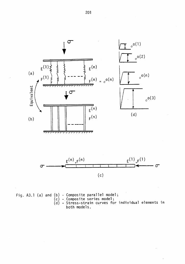
201

II IOo(2)

E(n)Ö. ----- ( )

I I = OO(n) · OO

II

oO—(3)M _ E00

<¤> F(“) (M(C)

Fig. A3.l (a) and (b) — Composite parallel model; M(c) — Composite series model;(d) — Stress-strain curves for individual elements in

both models. ‘

202

If 6$g)p is the plastic strain, then the elastic strain in the nth

element is expressed as,

(nlp = (nlpgij eij - eij (A3-3land, therefore, the elastic stress-strain law for the element can be

written as,

(nl - (nlp613 ‘ Dijksa (6ka ‘ 6ka ) (AM)

Defining a yield condition,

(nl (nl (nlF .. - .. - = A3.5l (ow oak] ) op 0 ( )

with Prager's translation rule,

= (VÜP A3 6oaij C eij ( · )

along with a flow rule,

·(nlp - l (nl (nl ·(nl613 ° [GY"13 (“ka 6ka ) (AM)

completes the formulation of basic equations. oij define the position

of the yield surface and op its expansion. K is the hardening modulus

and nij are the direction cosines.An elegant example of a parallel concept is the overlay model due

to Zienkiewicz et al. (l972,l978).

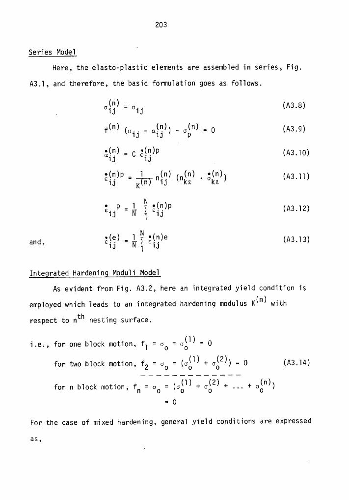
203

Series ModelA

Here, the elasto-plastic elements are assembled in series, Fig.

A3.l, and therefore, the basic formulation goes as follows.

(0) =1 61j 61j (A3.8)

(VI) _ (Ü) _ (Tl) = A3 gr (6111 611) ap 0 (.)•(0) - •(¤)Paij — C 6111 Q (A3-IO)•(¤)1> , l (0) (0) _ •(¤)(nkßE

p = l §E(")" (A3 12)ij N 1 ij ‘

and ;<<·=> = li ;<··>@ 016 16)* ij N 1 ij °

Integrated Hardening Moduli Model

As evident from Fig. A3.2, here an integrated yield condition is

employed which leads to an integrated hardening modulus K(n) with

respect to nth nesting surface.

i e for one block motion f = 6 = 6(A) = 0• •Q Q 1 O O

for two block motion f = 6 0 (A3 l4)’ 2 0 0 0 ‘

for n block motion, fn = 60 = (6é]) + 6é2) + ... + 6én))= O

For the case of mixed hardening, general yield conditions are expressed

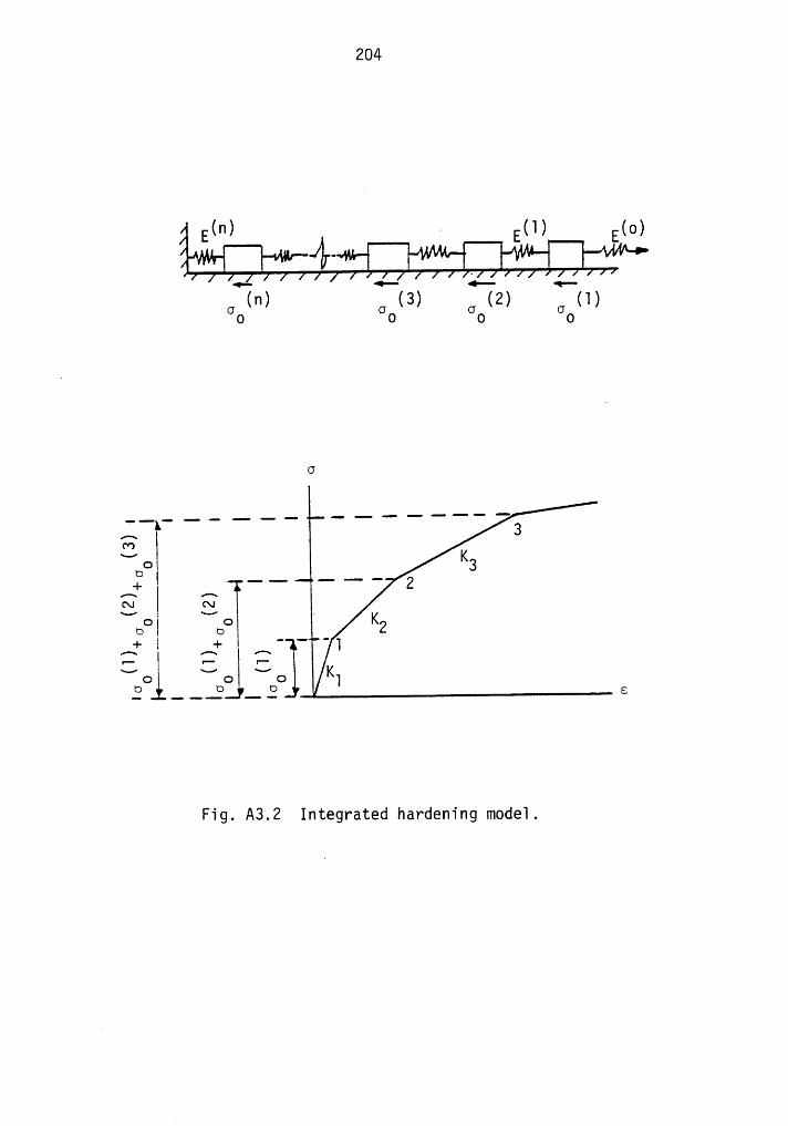
204

E(n)JIT

· EU) E(o)

'l> °”< > °— ‘”n 3 (2) (l)Go Oo Go Oo

~

L" ' ° ' ' " ”_-3°° KOO 3

+ ‘"° "' "" 2Q l Q K2Ä I ^+ 'l\-/iiE

..-2 ...2 3

Fig. A3.2 Integrated hardening model.

205

·_ (0) _ (0)2 -fo (cij aij ) op — 0(l) (l)2 -f] ' " Op '0_

(0) (ri)2 -_

fn (oij oij ) - op — O

Flow rule is given as,

EP. = 1 n.. (5.. n )1J 1J

1Jwhere,again, K(n) is the hardening modulus corresponding to nth nest-

ing surface.

A translation rule is employed which gives Ziegler's rule as a

special case.

Discussion5

Now, the difference in the three formulations becomes obvious. In

the first two models, the response of the system at any stress level is

the summation of the responses of the individual elements. with each

element, is associated a hardening modulus, K(n). 0n the other hand,

in the third model, hardening modulus at any stage K(n) is the inte-

grated behavior of all elements in yield state. In other words, in

the first two models, each nesting surface represents one element

representing one slip plane, whereas in the third model each nesting

surface corresponds to an integrated fraction of slipping elements with

respect to the total number of potential slip mechanisms which may

become active, should the collapse of the continuum occur. WG infer

that the first two models are microscopic in nature while the third

206

is macroscopic. And, here lies the fundamental difference between the

first two types of models, which are composite structure models, and

the third, which is an integrated hardening model.

Imagine a particulate system of l000 particles with each particle

making three contacts with adjoining particles. To form a series or

parallel model, ideally we shall need a combination of 3000 elements,

each maintaining a bookkeeping of what is happening at a particular

contact plane. To obtain the response of the system at any state, we

would extract information of its loading history from each element

individually and seek a combination in accordance with a parallel or

series arrangement.

In the integrated hardening model, we will seek to model the

behavior of all contact planes which have crossed the yield limit as_awholg_through a work hardening modulus. This modulus is constantly up-

dated as more and more contact points travel past their yield limit.

Thus, the work hardening modulus in the third model represents an

average property of the yielded portion of the system.

Qualitatively, first model is a stronger system while the second

model a weaker system. The third lies in between. It can be shown

that the first two models attain a steady state under cyclic loading

with no possibility of cyclic creep (Drucker, l98l).

These distinctions having been difficult to discern, several reportsi

demonstrate a confusion about the formulation of these models. For

example, it becomes clear that the foundations and the framework of the

paper by Prevost (l977) are those of the integrated hardening model and

not a derivative of all three models combined, as has been erroneously

207

mentioned by several researchers.

Again recently, Szavits-Nossan (l982) indicated that his

kinematic hardening model is based on Iwan's series model, whereas,

after examination it can be seen that it is a parallel model.

Examples are numerous, but it is not the intent of this note to

bring to readers' attention individual errors. If this brief exposi-

tion has clarified a subtle difference between two basic approaches

of formulating multisurface hardening models, the author would think

he has succeeded in his attempt.

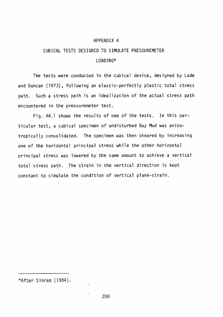
APPENDIX 4

CUBICAL TESTS DESIGNED TO SIMULATE PRESSUREMETER

LOADING*

The tests were conducted in the cubical device, designed by Lade

and Duncan (l973), following an elastic-perfectly plastic total stress

path. Such a stress path is an idealization of the actual stress path

encountered in the pressuremeter test.

Fig. A4.l shows the results of one of the tests. In this par-

ticular test, a cubical specimen of undisturbed Bay Mud was aniso—

tropically consolidated. The specimen was then sheared by increasing

one of the horizontal principal stress while the other horizontal

principal stress was lowered by the same amount to achieve a vertical

total stress path. The strain in the vertical direction is kept

constant to simulate the condition of vertical plane-strain.

*After Sinram (l984).

Ah 208

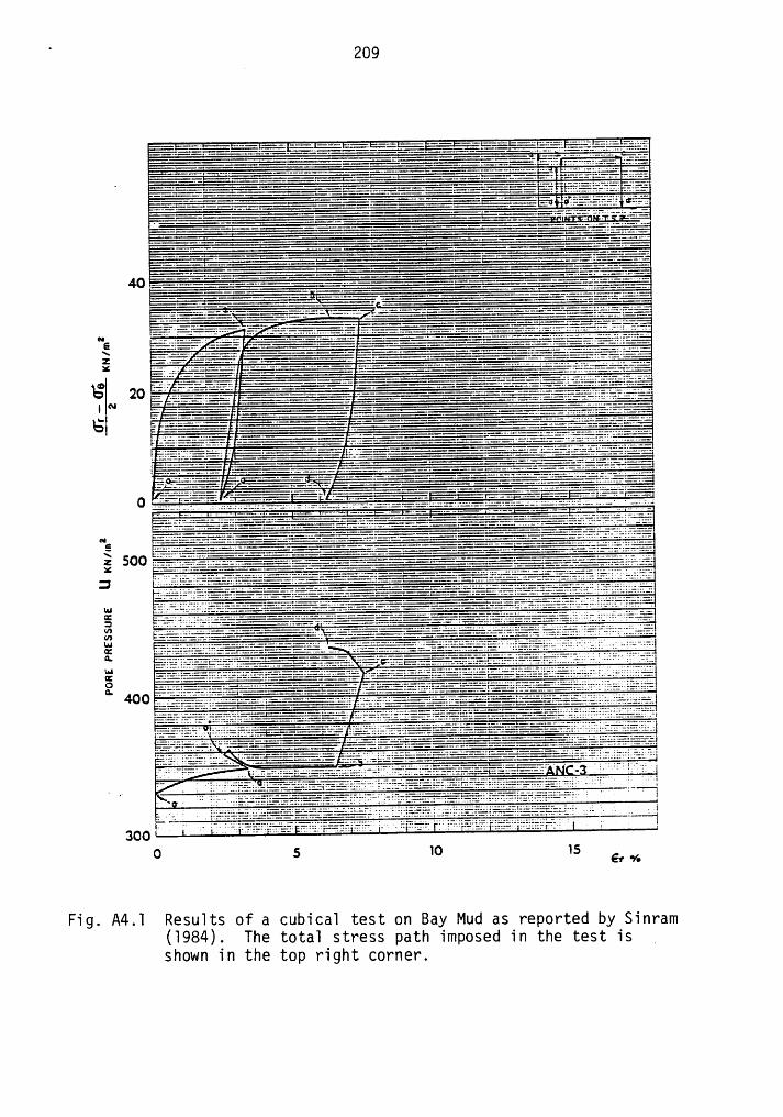
' 209

...... ...... ..—-•--—

—-•-—- -——— -·--— -———2i -;.:..,1 T"“l2Zil -2-'ZZLLT --2Z1 ·"$'é·?¢:-..:1-=———..-.-‘———„-;$-:1::--:f—=-———’—~-————=—·=·=·——·——f***?E?’iZ§E” =.-EEif.40

——.i*'-—-"°-—’Qf:—-——.._.._._.................-———_'—ä··-————·————~————·—.;.;—.....-.—-—+————_·;;·—f?;¢;·;.;——-i;;:—____—+:··—···—_.. .....·.._..··——;:¤f.-.2-..—..-.=-ff*ff“? T-————“°'%—;Z°———j··§.“

“_f?::f-;;;;‘ff€Qiiiiiiäffgee

I N g —-——:—'*"::—'f·;i;j;j;5;f;‘;;,;— EQ

*1*-—=’—’-T t- *· *--3-::;::.--...;Tit:.-fT:...ff:. .... ‘:’.T”.’jjfJL§II...I-.i.... .1..LI7;.I.L;11.ZI.Z°ITTZIZZL:ZZL?ZI.‘..-.l‘.1.I“'T;i1..:-;-;——--·:·—-—--:j;::r;;·j;:"ei;j;i;;·-L;.:1-:;

E -**:51-—-—-—·..1.I'..l..,....."“"'- Tl

V”:·*;‘*—·l·LIÄLL.:.*éE*i%E·LEE:‘.+.§iE§f?§%·E%é::—**‘LE‘^ EEä#‘===””‘—T~"”’='·=’ fiff:T;tiffit;tf‘‘‘.‘‘ffii? i

ar ;=::UI ....-...--.-..-- .----l·~-—--—;;—;;—_g;;;-5;;:;;; .„;:.::::.;::::::x::r;:;::::;:5:;ggg_{}§g;;;;_;;_{Z_¢Q;;3§}Zi{E?§iZ;g :¥%€E—·————::‘:?*-*'°“————”"'£‘*" ""f—'T”':.”j*:?EiE:”EE;?ifT:i:;i::1:iififi ii;fi‘.fii;:fff?G 499

'i;_fi‘=gj-igfil4 · ‘ ::2.;..i3*i·*5?€?äE5Eä?r?i€f’-:·:r;.;;„ _„· ’° 6 -

300 ‘Q 5 10 15 6, %

Fig. A4.1 Resu1ts of a cubica1 test on Bay Mud as reported by Sinram(1984). The tota1 stress path imposed in the testisshownin the top right corner.

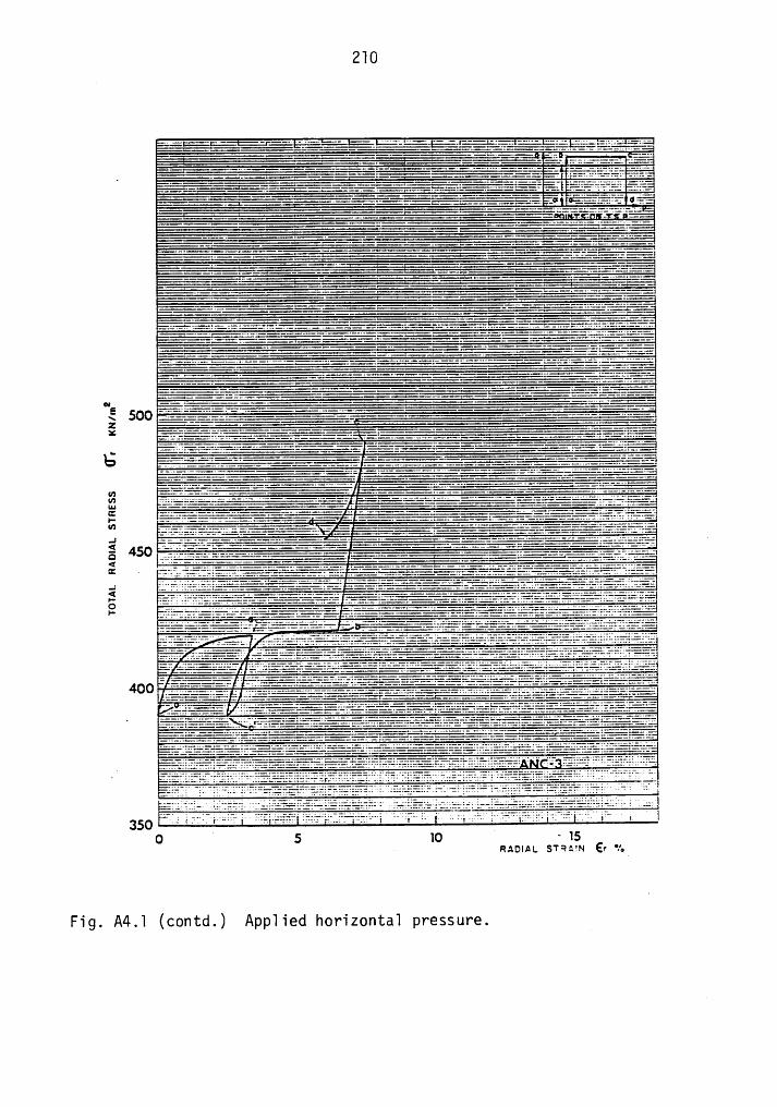
2 1 0

I: ..."=*-......22.-——-———°““ Ä;;.._.-T--2 II I “._“*-Ä;.-...IZ':-Ä*-;2?._.#———-—’ #--1.Q.IE' ’

ää-..;—„_._·—————-**·-*.._.-2——-*-‘-*4‘-..—.—::.=;.:;-:—;——._.-;Ä*-‘-.?.2;Ä‘*·—..—:;:.——E2=$1 :-2;: §

äi¤·————""""Ä'“"—°'-....2._...._..........."—;.'T"''—...—_——..2...""*—*·*-*-**-........'————-——'°....”"“°T:’i§:’:‘--**-—-—-——-——————-*-*-*-‘**·.__..-T-..=_..——-—-——2——-—-.-_ -*-_..-T-. -,.1.*T ·- ·=—¢;_=-*-;:6* · TT

1....-‘—';._...—‘-"“I......_...*"""—————————""*‘——.„.—.*—=—‘—*—"..~——;?;—=___·————".?;;;‘;“f—+—f_;

“'“"-f"Ä._.... ... .'.....“"".. -.-°.f-.:Ä**-*-*‘-‘*‘...'“.'L.°°Z—ß..-°°'—“-‘.;.-T-_.--T—‘._..._....Ä--2-*—-‘-Ä:-T-*"""'"'—=-———-·—-..........2_...-‘————·-—T--'“‘:„>—-2;*-*‘

————·-—---—-'—'=""’—---—"——"°'Ä*-·—:'"—’-Ä"I_"’°°-—*-—-°'f‘—·'-—Ö’Ä?•—Ä*——-—.."“"Ä‘?—-——.;-}.'—”_.—'"; "'”——-·-—-_.'ÖÜ.....“—J°——*‘*‘.;"l**-‘:¥—”“”-TT-°"·Ä__'Z.Z-—.°_°7.l—;’——-Ä.“’...“'”:.‘“-*-‘———-—.I.'“..I“'I.’_.lä$§i+-liizä

'I.....”' ”„———”—'Ü’...°“'._“'I ”......“*-Ä“_......'”"°“-‘Ä_.........-Ä"”°'“°°°.-._.'°-.I ”°..’.'°'*-."._..."“__..-*-""“Ä;——‘...:"‘-I2.i;E-Ä;IIf"I’—°"'“;:·-*-*-Ä‘-*"'°““—..""..———“""". ;—-—.._—-—*·*-Ä-•--—-————-——-—“""'“_ZÜ';_T*·T·'°“Ä

-*:2_-——T°fÄ———*’g———I-l”'”———-——·—““———f—j—————':Ä————————w—:-""""'_-—--i""""'"--’"°°-_:—*-f—j„E_..·;_:‘i.3E:“;:_i..:‘_..;_"‘.;.""..”::....—f.—-.Z....:»_\ 5QQ T .-.... .z .;.··—.:··—...-.:Ä—--Ä·-——-Ä-* -———-""ÄÄ—-—-!

S g

gg 1 -—i’1i1=—.”—f"”:-.Q —";——..-Ö'. Ü;Ä————————...äZ}

450 eiT¤¢·<

'“' """°"""'-"""f""f'f"'"‘ff"' '°"‘f"ff"fff'“"'”"[°'°‘”"f""°'f;;f;;T'_;§f:_;;;;f:"“h• IfT T ' . IT'ITL1TTffZ‘.L'TfTT‘f"'.ff..ZT;' fZLff.f.1';TfI'J„°1l'.T'.f.'.Zfff.ffti-T-: :;;:;-74-Trtggc *1;;:;; *;-1:; ;.:;*:;:;;::::;::.*‘ ;t::1:;-.:;i::‘;;:i::;T;:t:;i::::ii "Z'L.-. . . -...-.4 ..--1*

I eéereäazej

400 :-:::::::2;-.:;:j

'Ä'” .’ :111Zfläié0

I S 10 I · 15- Raum. s‘r=z:m Ey 21,*

Fi g . A4 .1 (contd .) App1ied hori zonta1 pressure.

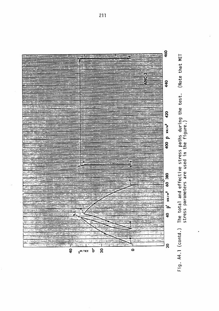
~:T‘:C‘ :2.. 8

Q *2-

———-2.-.-..._____,_

;.—-;i·*———·—-i:-_;;———=—"é::**‘

-TQ

-i—;;-T,.'-:1?1——-—-*-22-··-2-2:

.5**-:_-—_l·i—i-__i—·l"'*

4-,

22 22

‘ ;_;;3;;;;;j=¢..-;-:::;:„?;.,;*€+-:=*;

$

__ =;?.i5_,;;;·:—;-——-—Q__*:_Q______...-..-—.*****—————-:

V

---iU_EL;_—°——”°°"T'

U}

—··—-i--L

‘: ^

[5:;.:;: —-——..-...-—-.....,__

’"*—-—-—-·"-=‘?=-**;:.-:—..1'T;·,_§‘.- an••- •

"’“f2;=-*—————.._j;_’;_*‘;E S- <v

__*é;:;.——_-;;—__:—é

3 L——— " cn

;:I'T.—·—·—·---—-

4-*"¤ GJQC

"*===—:..*·=E*==‘*

42W"’ CGJ ·•·-

·~~?';;.‘;*—=—:-*=-i}-——-——”

""”¤

.*;2:-:2-2-*2;'—25*:'2m Q)

gg-;

>

—E}..Zl¥.ZL§_ 8•'¤

°"‘ ‘^

*=*=;:;:;:"'-A-;i1?iEt2*=’—:=¢?E?—CT-; '° E S-CU

-;*;;*.::.75}.;;-;.éä7;::i;£_r_;;;T___g..:g._j;:_**;___;***¤1'¤¤=-:1*:**·?EE?-T;.§}Q?g;<r:;:.—:;;_—l____z

‘¤ ¢¤gg

;j:;;~1;;;:;::._,__________ '°?iI‘,_-.:F¥{;§§- ggg:.¤§;2?:::;;1;;_:::.-_:'ffj:*_:g·:3¢*¥1'f?:‘-::::·„:;;:;;éj§5_’j__

• (U Q¤- 4-* '

··.”"?ZEé.-.””C?*¥ééi€E;5:>.:;ZÄl:??Il?;Ii;f€’$E§fi**°=**¤=— Q W

~- li? ‘***···"':r—————·————........;E>*; · .;,_ "‘°"‘*·*··--·*¢===*==:§?';T—§;=E**=¤*r=:::—.éé&3;**·

GJ

:-Ii;:7i;f*=*E€.§—•i;;;;*:1::;.:i§i;llIiiiZlTT;;i**

2 GJ S-.C -4->

, QQji'“"·‘=°*>=’—¥iCi5E*EQ$:§?6;::::;:§}ÄÄ}ÄTLJ'“’TTEf_* Zäéii-ä??:éé;éLé;;;:::;:

JT W^

· :::2;.Ii::€E?:§§?§§}1:::-;-;_•;;_-:.T”,;fffff‘¢¢

*=:=g;.-.;;;.„._; _ __ Z ; _ " 4;

** - ·---..:::::;-;:1;;--gg_*;— ·;;;;E- ·- _; _T·-.g g __;,‘:__:;;:E....L:j·i::;gm *};*:;::::::1 ** *”*E::*‘:::*‘::¥::;:*O

'· :· .. . „_, 8” O(Q sz

I"

<r

—<UvZZ

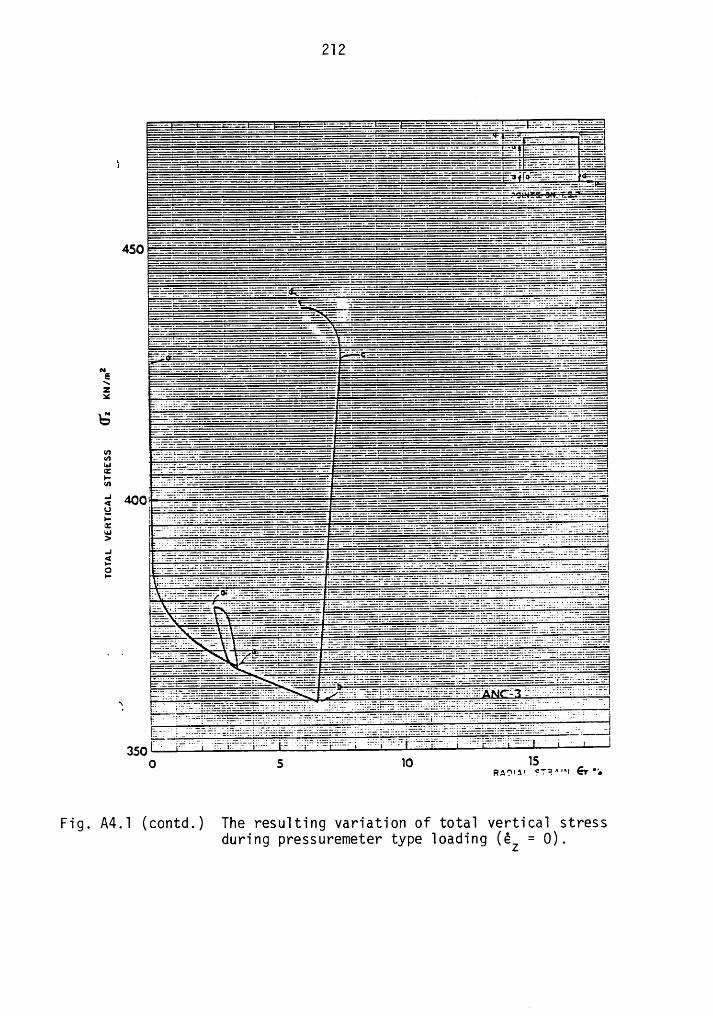
2l 2

iéäéäräii "*——:_1_—;:-;;+1:*--*‘‘‘‘*.;>-—-—:;i;;*——————————."1;:;;;*..1-+..1**.;;;+*--*1‘——·;;;#le7zääewée

...T.l—’;-;.·——T“'"::.v·-=——:'“*—***.._ «— ..T’...+;’."?é» ’i<£·ä;é?ää* °“?&—**__.———*—··‘.___-...·—”*—_‘"“*—¤—-———————°—’**""—.:.._.'·—··“'—'IT;";;éfäFäé_

‘”'°' ' "”"_-——-———"’_'°""'""""——————“""”‘"'——————"°""_’..°’°;——T;j_;—--jj_Z¢;>———g;g;;;;§;I_;_-*:*1;:1;--—·-—-———;**—T*‘?:—1_—=é;11:1.—*=—-—;—........**_1;i?4501T:_—;11·—_;:.—;:';::_”"°°‘-T1·-—··-——·——·—°—'—_—°1.-..i*——————*_1jr_-ij_i""‘—j;l·-_?.r—

--_......„:._=;;*:i::.:—.._*;;*.T..;?_:*;.;_E&ä;€;ä%;ii;,

Äl".———-—·———.‘*‘*T..‘l.T.'—':*·*—'*——*‘—‘......__'"_""’”'—°"*.—;‘;**ii?-—-°-i——-—-——.....r—********1—;—.:“...Ü—.,f°E

* _________________Z +===-———:_**;—'*‘.._._—-—;—·‘=,.;...=*-¥§fI€i'·?Z?E..'*’;*:'.—Ü..f*'****——_....-....._.**—.·.....**—*‘:_.,_ _} ""'—"°"Z-»-Z G’-1"'-—i—'""'°'""-T'f;§Q_:E—___;-_;:-;:-;L7;;_—---•*'

11111 1*1111-1-1-—1—11 ”“'———————————·—*‘*‘—--———‘“'“‘__„'IQé*

Zi 1;-s-*1-:,;;?**‘—-.:::;:.1-w 1*-Lnl ·r;;;;;;;,—::;:t:;..._...***··•‘•·*:‘**.i."'*' ”‘*‘*"‘""'°°-'-——-——'l’-—;"-L——~'——————'—":_-7:EE:;:.r:rt:::::;::t::?.—_ _·_;:·:·+· ,l;...m_.l"""*‘X..IT .17-T'-°i'l————-'iZ'i··—·— ·—·—-—-·-·-·—-··:·_··;;:Minn;-:";;·_F- ; _1 ·:;;:;::::*·—...._...*"""*7 -I-:_Z-'1‘i‘'°—-+”—i—;}_···;::;:,1;:;:::*;:1:."’a'

400; *;*:1; —;;.;+——*‘*.._-——_-.*.g-——-.—*‘—..„...9}·— · _.;?5it.¢:::;::r:t:;:*;::::rit.;: ‘;‘ ‘ Z "ZYTI•— , 11* :*;*—::.-i*—§:—:———'**—':T:-.?*?;•_:—;·*:_:1.T__l_1·:.:*..:'ia;.?2;r<*1;;=<=Z1 ...—11·..11i1:.1i1T1.:1.:1.;.—.-•-1---1„~-—-- --·-—-··—~—··—--—-—-·—v;r··· —··;;;;,;;·::;;;;::.;..-;:;:.2% .-.1f"1-J-ll

·· ::~;;l:--=-——*t_.“'ZT”—'_— ;v==>«#=2=*222;=—*;·

·‘E;;;;;;:·;;;;;

;2;;;;;;:*e&:a—:a· *:-:2;%.**;*;..=:.=;?:¥s;:+ä:;;;§;iEj;;eäiäggjgüggylé

YZ r:;ä;i@2;-*2132 ÜEE1?1"1T P ‘ ·ä?¥¥17Y¥%Z%ä*—%**?¥—**¥?§?%ias.

‘ 7** 2*;

lS0 5 10 n.¤0•:·_ sv=z····« Gr';

Fig. A4.l (contd.) The resulting variation of total vertical stressduring pressuremeter type loading (éz = O).

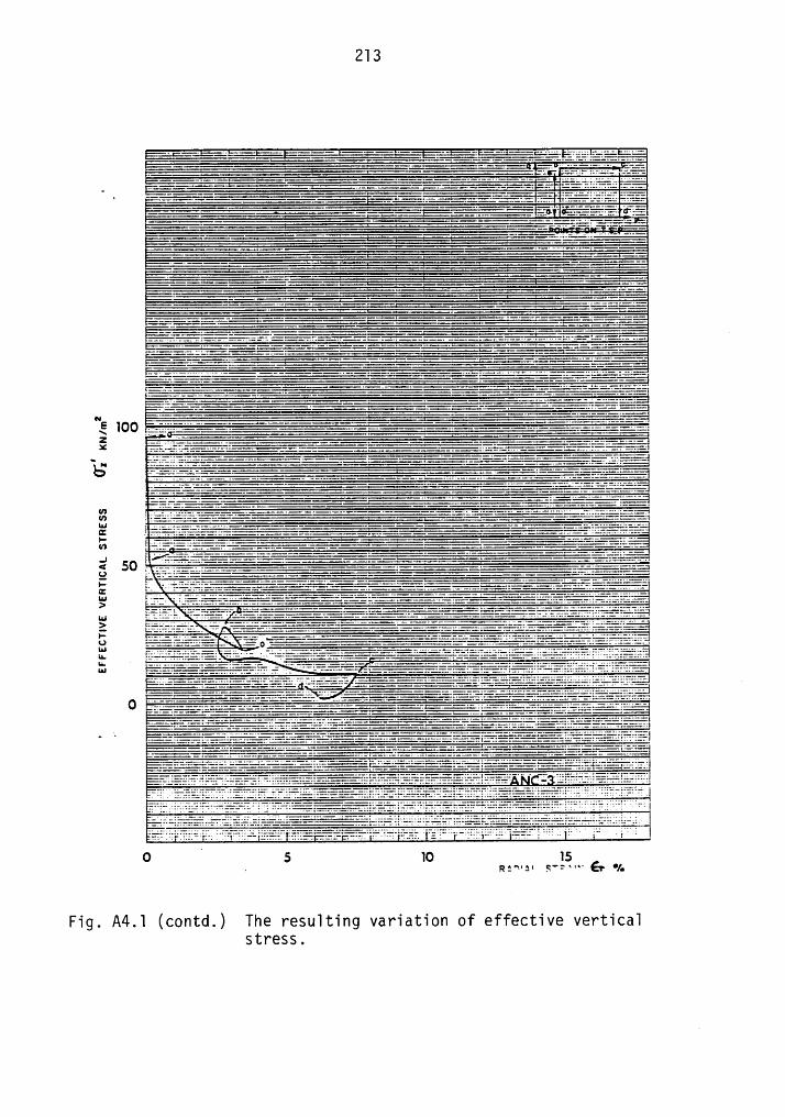
213

—'=·—‘°°°° N- _Z—-—————-——'°"°‘ ...°i’“T'i·;%é.;äé%é;ä4FilI-—·;_—·-——·—·-—i·l····—·———···—·——·——·—·····—·—·—i···——·—·——··—··———···· ——· 3 :2;.;;.;.::.;;;il_ E $$111TIT;·

‘ ä>=_——_—————;—-————‘*T_°——”—‘——°°_——————°_°i1”-°—°——..;..——”?£“ é N:

EäääääääääEääääääEääääääääääääääääää*'°—..··——·————·T·-T*—·T·..._._’T’°"“’.._...._"“““'“°'“—“"—“_.._T··:;..._.._""'“"”'“'“°“““"'_.“'°——’"T·T*T‘T'I_.."'”'

"—:'jj:—T;—.'l——-ET—. ”_"-—"""‘——-—·*’*"‘“·-—·—-—‘N’~—-——-——""'_...."""......——-—-—————""-"“"“__...;....‘‘‘‘-’===¤——._......; "”“

...—?§ —.._..*‘—‘-——°—..._.—"-‘——"·”;;—Ü--—-————........—";” ”L_—_„..°_‘”—”“‘;...._—_....."‘—"‘”"”°-””_”.......”-——'”——‘"""‘N——°—..._..”‘_—————.=.·””Ä;_::Ä;._’_"————°:Ä‘—‘¥___. _“......°'“'—.;;.'""‘_""°"'“"'°°°""'.__...;.L-————-—·"'_lI'_:—;"..."'““

; °° ETE-—————TT-———-———·———·—·—·———··;‘TTT‘T——-———N-————TT—————————·‘Ti‘;‘NT"‘·—··N:—·:iiL:;iiT=== L;..Ü

‘h"

(0 1;:*':;*.trr;t"‘*...*;N".....;;.°.:•;·tt.*‘57..-——-l-~—..‘_"‘:.—.."’.........."‘”_*‘—"“.......;..‘*"’....""‘“i"....."‘N..;......i"_."‘ ‘ " jf __

' ..T'ZI:'.flZ'.;.

E—.>

ääeiezääzg "§;-—TI‘L—‘"·-l-"""=—·—————‘......."‘‘“ ”"‘....———-——— ;...=‘——’?:Ee2 ‘ ‘p:3¤.

TEN¤0

A5 10 15

~ R1""3' S"'=""€1* ‘/•

Fig. A4.1 (contd.) The resu1ting variation of effective vertica1stress.

Documents

ANALYSIS OF THE PRESSUREMETER TEST BY … · CHAPTER l INTRODUCTION Almost thirty years have passed since the first practical version of the pressuremeter was introduced by Menard