Analysis of Variance (ANOVA tests) - unitn.it · Analysis of Variance (ANOVA tests) University of Trento - FBK 16 March, 2015 (UNITN-FBK) Analysis of Variance (ANOVA tests) 16 March,

Analysis of Variance (ANOVA tests)

University of Trento - FBK

16 March, 2015

(UNITN-FBK) Analysis of Variance (ANOVA tests) 16 March, 2015 1 / 56

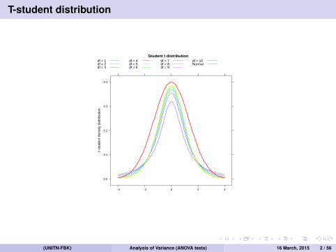
T-student distribution

Student t distribution

t−st

uden

t den

sity

dis

trib

utio

n

0.0

0.1

0.2

0.3

0.4

−4 −2 0 2 4

df = 1df = 2df = 3

df = 4df = 5df = 6

df = 7df = 8df = 9

df = 10Normal


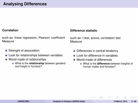
Analysing Differences

Correlation

such as: linear regression, Pearson’ coefficientMeasure

Strenght of association

Look for relationships between variablesWorld made of relationships

What is the relationship between genderdand height in humans?

Difference statistic

such as: t.test, anova, correlation testMeasure

Differences in central tendency

Look for difference in variablesWorld made of differences

What is the difference between heights ofhuman males and females?


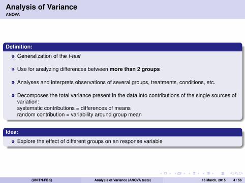
Analysis of VarianceANOVA

Definition:

Generalization of the t-test

Use for analyzing differences between more than 2 groups

Analyses and interprets observations of several groups, treatments, conditions, etc.

Decomposes the total variance present in the data into contributions of the single sources ofvariation:systematic contributions = differences of meansrandom contribution = variability around group mean


Analysis of VarianceANOVA

Definition:

Generalization of the t-test

Use for analyzing differences between more than 2 groups

Analyses and interprets observations of several groups, treatments, conditions, etc.

Decomposes the total variance present in the data into contributions of the single sources ofvariation:systematic contributions = differences of meansrandom contribution = variability around group mean

Idea:

Explore the effect of different groups on an response variable


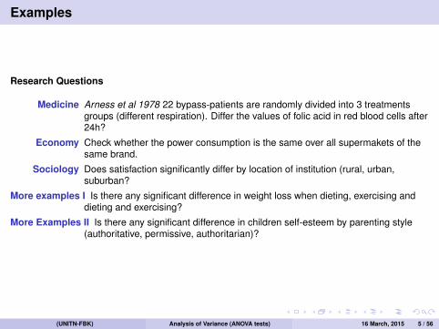
Examples

Research Questions

Medicine Arness et al 1978 22 bypass-patients are randomly divided into 3 treatmentsgroups (different respiration). Differ the values of folic acid in red blood cells after24h?

Economy Check whether the power consumption is the same over all supermakets of thesame brand.

Sociology Does satisfaction significantly differ by location of institution (rural, urban,suburban?

More examples I Is there any significant difference in weight loss when dieting, exercising anddieting and exercising?

More Examples II Is there any significant difference in children self-esteem by parenting style(authoritative, permissive, authoritarian)?


A working example

Example

Let’s analyze the Cushings dataset from the package MASS.

Info Cushing’s syndrome is a hormone disorder associated with high level of cortisolsecreted by the adrenal gland.

Variables Type: Categorical, define the underlying type of syndromeTetrahydrocortisone: Numerical, urinary excretion rate (mg/24h)Pregnanetriol: Numerical, urynary excretion rate (mg/24h)

Aim Find whether the 4 groups are different with respect to the urinary excretion rateof Tetrahydrocortisone


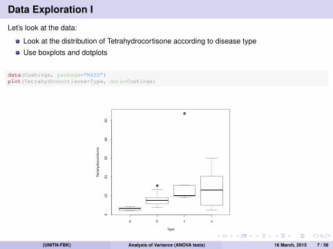
Data Exploration I

Let’s look at the data:

Look at the distribution of Tetrahydrocortisone according to disease type

Use boxplots and dotplots

data(Cushings, package="MASS")plot(Tetrahydrocortisone~Type, data=Cushings)

●

●

a b c u

010

2030

4050

Type

Tetr

ahyd

roco

rtis

one


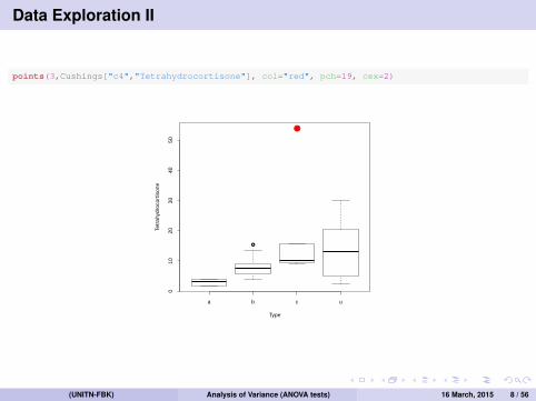
Data Exploration II

points(3,Cushings["c4","Tetrahydrocortisone"], col="red", pch=19, cex=2)

●

●

a b c u

010

2030

4050

Type

Tetr

ahyd

roco

rtis

one

●


ANOVA

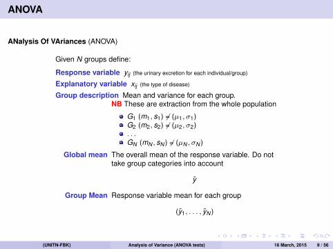
ANalysis Of VAriances (ANOVA)

Given N groups define:

Response variable yij (the urinary excretion for each individual/group)

Explanatory variable xij (the type of disease)

Group description Mean and variance for each group.NB These are extraction from the whole population

G1 (m1, s1) 6= (µ1, σ1)G2 (m2, s2) 6= (µ2, σ2). . .GN (mN , sN ) 6= (µN , σN )

Global mean The overall mean of the response variable. Do nottake group categories into account

y

Group Mean Response variable mean for each group

(y1, . . . , yN )


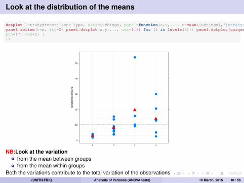
Look at the distribution of the means

dotplot(Tetrahydrocortisone Type, data=Cushings, panel=function(x,y,..., m=mean(Cushings[,"Tetrahydrocortisone"])){panel.abline(h=m, lty=2) panel.dotplot(x,y,..., cex=1.8) for (i in levels(x)){ panel.dotplot(unique(x[x==i]),mean(y[x==i]),col="red",pch=17, cex=2) }})

Tetr

ahyd

roco

rtis

one

0

10

20

30

40

50

a b c u

●●●●●●

●

●●

●●

●

●●●

●

●●●

●

●

●

●●

●

●

●

NB:Look at the variationfrom the mean between groupsfrom the mean within groups

Both the variations contribute to the total variation of the observations(UNITN-FBK) Analysis of Variance (ANOVA tests) 16 March, 2015 10 / 56

Anova

Take into account variances

Anova partition the sums of squares (variance from the mean) into:

Explained variance (between groups SSb)Systematic variance, it reflects differences among groups due to the experimental treatment ofcharacteristic for group membershipThis is the sum of square between groups, hence the squared differences between each individualgroup mean from the grand mean

Unexplained variance (within groups SSw )Random variance, or noise. It reflects the variance from the mean between individuals in the samegroup.Sum of squares of the differences of each individual from the individual’s group mean

The linear model conceptually is:

SSt = SSb + SSw


ANOVA: variances

Recall the formula of variance:

σ2 =

∑(x − x)2

N − 1

We can rewrite it using the Sum of Squares and the degree of freedom as:

σ2 =SSdf

Hence:

Between SSb =N∑

i=1

ni (yi − y )2

In order to take into account the different sample size in each group, note theweight ni . Groups with more observation are weighted more heavily.

Within SSw =N∑

i=1

ni∑j=1

(yij − yi )2

Total SS =N∑

i=1

ni∑j=1

(yij − y )2 Deviation of each individual from the overall average


ANOVA

ANOVA Tests

Assumptions:Observation over groups are indipendentObservations for each group come from a gaussian distributionVariances should be homogeneous

H0µ1 = µ2 = ... = µN

H1 = not(H0)At least 2 means over all groups should be different

Compute the F-statistic for N groups and n observation:

F =SSb/(N − 1)SSw/n − N

Comparing variation between groups and variation within groups. If the null hypothesis istrue, then the test statistic F has an F-distribution F (dfb, dfw )

Degree of freedom:Between dfb = N − 1

Within dfw = n − N

There is any significant difference between at least two of the groups in variable x


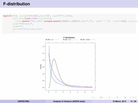
F-distribution

xyplot(Y~X, groups=df1+df2,data=df, type="l",lwd=2,auto.key=list(TRUE,columns=3,text=paste("df1,df2",unique(paste(df$df1,df$df2,sep=",")), sep=" = "), lines=TRUE, points=FALSE ),

ylab="Density",xlab="",main="F-Distribution",)

F−Distribution

Den

sity

0.0

0.2

0.4

0.6

0.8

1.0

1.2

0 1 2 3 4 5 6

df1,df2 = 1,1 df1,df2 = 2,5 df1,df2 = 10,20


Test variable F:

Fobs = SSbetween/(N−1)SSwithin(n−N)

If Fobs > θ or pobs < α reject H0If Fobs < θ or pobs > α accept H0

Accept H0 ⇒ µ1 = µ2 = ... = µNReject H0 ⇒ µi 6= µj

NB: i and j could be any couple of groups!


A working example

Example

Let’s analyze the Cushings dataset from the package MASS.

Variables Type: Categorical, define the underlying type of syndromeThis is the grouping variable N = 4 Tetrahydrocortisone: Numerical, urinaryexcretion rate (mg/24h); the response variable y

Aim Find whether the 4 groups are different with respect to the urinary excretion rateof Tetrahydrocortisone

Compute the overall mean y :

mean(Cushings$Tetrahydrocortisone)

## [1] 10.456

Compute the mean for each group yi

tapply(Cushings$Tetrahydrocortisone, Cushings$Type, mean)

## a b c u## 2.9667 8.1800 19.7200 14.0167

Compute Degree of freedom dfb, dfw :

length(levels(Cushings$Type)) - 1 ## df_1nrow(Cushings) - length(levels(Cushings$Type)) ## df_2

## [1] 3## [1] 23


Manual Computation

Compute SSb and SSw and the f statistic:

SSb <- sum(table(Cushings$Type)*(tapply(Cushings$Tetrahydrocortisone, Cushings$Type, mean) - mean(Cushings$Tetrahydrocortisone))^2)SSw <- sum(unlist(by(Cushings, Cushings$Type, function(x){sum((x$Tetrahydrocortisone - mean(x$Tetrahydrocortisone))^2)})))f <- (SSb / 3) / (SSw / 23)

Compute the p-value = P(F ≥ 3.2)

pvalue <- df(3.2, df1=3, df2=23)

Define a threshold α that if pobs ≥ α we reject H0. Normally α = 0.1, 0.05, 0.01

pvalue

## [1] 0.041074


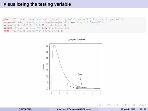
Visualizeing the testing variable

plot(df$X, df$Y, yla="Density", xlab="", type="l", main="F(3,23), f=3.2, p=0.041")polygon(x=c(x, rev(x)), y=c(rep(0,length(y)), rev(y)), col="grey80")arrows(x0=2, x1=3.2, y0=0.05,y1=0, lwd=1.5)arrows(x0=3.5, x1=3.8, y0=0.2,y1=0.01,lwd=1.5)text(x=2,y=0.05,labels="f",pos=3,cex=1.8)

0 1 2 3 4 5 6

0.0

0.1

0.2

0.3

0.4

0.5

0.6

0.7

F(3,23), f=3.2, p=0.041

Den

sity

f

pobs


Let R work for us

How to compute evertything in R?

myanova <- aov(Tetrahydrocortisone~Type, data=Cushings)summary(myanova)

## Df Sum Sq Mean Sq F value Pr(>F)## Type 3 894 297.8 3.23 0.041 *## Residuals 23 2124 92.3## ---## Signif. codes: 0 '***' 0.001 '**' 0.01 '*' 0.05 '.' 0.1 ' ' 1


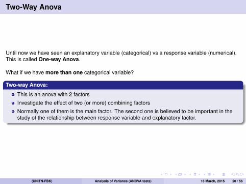
Two-Way Anova

Until now we have seen an explanatory variable (categorical) vs a response variable (numerical).This is called One-way Anova.

What if we have more than one categorical variable?

Two-way Anova:

This is an anova with 2 factors

Investigate the effect of two (or more) combining factors

Normally one of them is the main factor. The second one is believed to be important in thestudy of the relationship between response variable and explanatory factor.


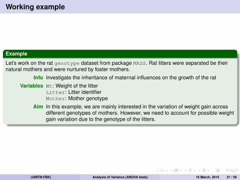
Working example

Example

Let’s work on the rat genotype dataset from package MASS. Rat litters were separated be theirnatural mothers and were nurtured by foster mothers.

Info Investigate the inheritance of maternal influences on the growth of the rat

Variables Wt: Weight of the litterLitter: Litter identifierMother: Mother genotype

Aim In this example, we are mainly interested in the variation of weight gain acrossdifferent genotypes of mothers. However, we need to account for possible weightgain variation due to the genotype of the litters.


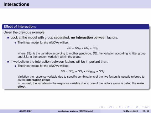
Interactions

Effect of interaction:

Given the previous example:

Look at the model with group separated: no interaction between factors.The linear model for the ANOVA will be:

SS = SSM + SSL + SSE

where SSm is the variation according to mother genotype, SSL the variation according to litter groupand SSE is the random variation within the group.

If we believe the interaction between factors will be important than:The linear model for the ANOVA will be:

SS = SSM + SSL + SSM×L + SSE

Variation the response variable due to specific combinations of the two factors is usually referred toas the interaction effectIn contrast, the variation in the response variable due to one of the factors alone is called the maineffect.


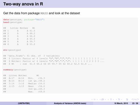
Two-way anova in R

Get the data from package MASS and look at the dataset

data(genotype, package="MASS")head(genotype)

## Litter Mother Wt## 1 A A 61.5## 2 A A 68.2## 3 A A 64.0## 4 A A 65.0## 5 A A 59.7## 6 A B 55.0

str(genotype)

## 'data.frame': 61 obs. of 3 variables:## $ Litter: Factor w/ 4 levels "A","B","I","J": 1 1 1 1 1 1 1 1 1 1 ...## $ Mother: Factor w/ 4 levels "A","B","I","J": 1 1 1 1 1 2 2 2 3 3 ...## $ Wt : num 61.5 68.2 64 65 59.7 55 42 60.2 52.5 61.8 ...

summary(genotype)

## Litter Mother Wt## A:17 A:16 Min. :36.3## B:15 B:14 1st Qu.:48.2## I:14 I:16 Median :54.0## J:15 J:15 Mean :54.0## 3rd Qu.:60.3## Max. :69.8


Two-way anova in R

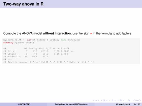
Compute the ANOVA model without interaction, use the sign + in the formula to add factors

myanova.noint <- aov(Wt~Mother + Litter, data=genotype)summary(myanova.noint)

## Df Sum Sq Mean Sq F value Pr(>F)## Mother 3 772 257.2 4.25 0.0091 **## Litter 3 64 21.2 0.35 0.7887## Residuals 54 3265 60.5## ---## Signif. codes: 0 '***' 0.001 '**' 0.01 '*' 0.05 '.' 0.1 ' ' 1


Two-way anova in R

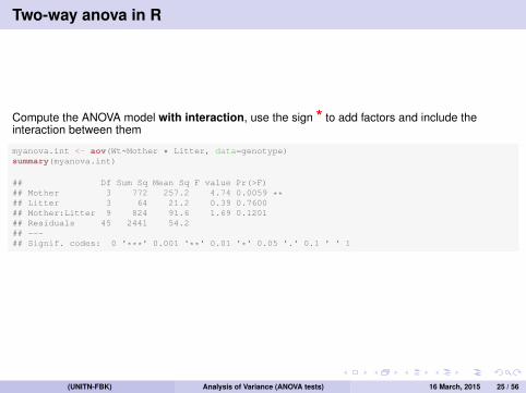
Compute the ANOVA model with interaction, use the sign * to add factors and include theinteraction between them

myanova.int <- aov(Wt~Mother * Litter, data=genotype)summary(myanova.int)

## Df Sum Sq Mean Sq F value Pr(>F)## Mother 3 772 257.2 4.74 0.0059 **## Litter 3 64 21.2 0.39 0.7600## Mother:Litter 9 824 91.6 1.69 0.1201## Residuals 45 2441 54.2## ---## Signif. codes: 0 '***' 0.001 '**' 0.01 '*' 0.05 '.' 0.1 ' ' 1


Check the assumptions

Recall:

Assumptions:Observation over groups are independentObservations for each groups come from a gaussian distributionVariances should be homogeneous


One more example

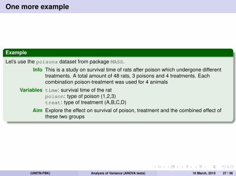
Example

Let’s use the poisons dataset from package MASS.

Info This is a study on survival time of rats after poison which undergone differenttreatments. A total amount of 48 rats, 3 poisons and 4 treatments. Eachcombination poison-treatment was used for 4 animals

Variables time: survival time of the ratpoison: type of poison (1,2,3)treat: type of treatment (A,B,C,D)

Aim Explore the effect on survival of poison, treatment and the combined effect ofthese two groups


Explore the data first

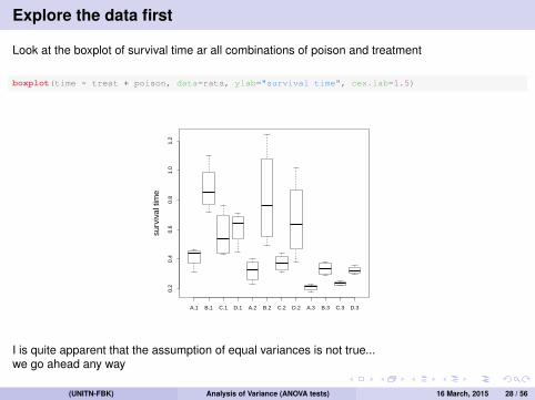
Look at the boxplot of survival time ar all combinations of poison and treatment

boxplot(time ~ treat + poison, data=rats, ylab="survival time", cex.lab=1.5)

A.1 B.1 C.1 D.1 A.2 B.2 C.2 D.2 A.3 B.3 C.3 D.3

0.2

0.4

0.6

0.8

1.0

1.2

surv

ival

tim

e

I is quite apparent that the assumption of equal variances is not true...we go ahead any way


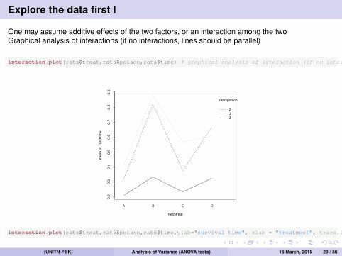
Explore the data first I

One may assume additive effects of the two factors, or an interaction among the twoGraphical analysis of interactions (if no interactions, lines should be parallel)

interaction.plot(rats$treat,rats$poison,rats$time) # graphical analysis of interaction (if no interactions, lines should be parallel)

0.2

0.3

0.4

0.5

0.6

0.7

0.8

0.9

rats$treat

mea

n of

rat

s$tim

e

A B C D

rats$poison

213

interaction.plot(rats$treat,rats$poison,rats$time,ylab="survival time", xlab = "treatment", trace.label="poison", cex.lab=1.25) # you can add options to make a nicer output,


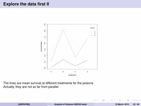
Explore the data first II

0.2

0.3

0.4

0.5

0.6

0.7

0.8

0.9

treatment

surv

ival

tim

e

A B C D

poison

213

The lines are mean survival at different treatments for the poisonsActually, they are not so far from parallel


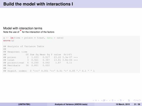
Build the model with interactions I

Model with interaction termsNote the use of * for the interaction of the factors

g <- lm(time ~ poison * treat, data = rats)anova(g)

## Analysis of Variance Table#### Response: time## Df Sum Sq Mean Sq F value Pr(>F)## poison 2 1.033 0.517 23.22 3.3e-07 ***## treat 3 0.921 0.307 13.81 3.8e-06 ***## poison:treat 6 0.250 0.042 1.87 0.11## Residuals 36 0.801 0.022## ---## Signif. codes: 0 '***' 0.001 '**' 0.01 '*' 0.05 '.' 0.1 ' ' 1


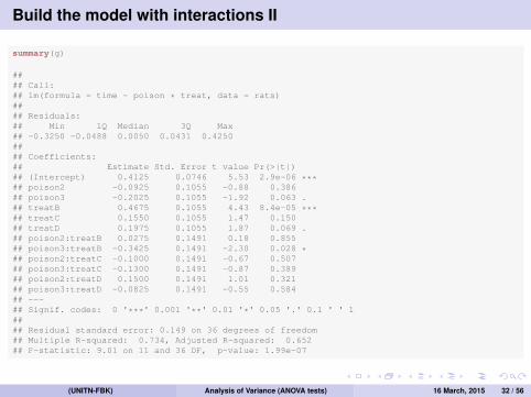
Build the model with interactions II

summary(g)

#### Call:## lm(formula = time ~ poison * treat, data = rats)#### Residuals:## Min 1Q Median 3Q Max## -0.3250 -0.0488 0.0050 0.0431 0.4250#### Coefficients:## Estimate Std. Error t value Pr(>|t|)## (Intercept) 0.4125 0.0746 5.53 2.9e-06 ***## poison2 -0.0925 0.1055 -0.88 0.386## poison3 -0.2025 0.1055 -1.92 0.063 .## treatB 0.4675 0.1055 4.43 8.4e-05 ***## treatC 0.1550 0.1055 1.47 0.150## treatD 0.1975 0.1055 1.87 0.069 .## poison2:treatB 0.0275 0.1491 0.18 0.855## poison3:treatB -0.3425 0.1491 -2.30 0.028 *## poison2:treatC -0.1000 0.1491 -0.67 0.507## poison3:treatC -0.1300 0.1491 -0.87 0.389## poison2:treatD 0.1500 0.1491 1.01 0.321## poison3:treatD -0.0825 0.1491 -0.55 0.584## ---## Signif. codes: 0 '***' 0.001 '**' 0.01 '*' 0.05 '.' 0.1 ' ' 1#### Residual standard error: 0.149 on 36 degrees of freedom## Multiple R-squared: 0.734, Adjusted R-squared: 0.652## F-statistic: 9.01 on 11 and 36 DF, p-value: 1.99e-07


Build the additive model I

Model without interaction term. Only additive effect.

g_add <- lm(time ~ poison + treat, data = rats)anova(g_add)

## Analysis of Variance Table#### Response: time## Df Sum Sq Mean Sq F value Pr(>F)## poison 2 1.033 0.517 20.6 5.7e-07 ***## treat 3 0.921 0.307 12.3 6.7e-06 ***## Residuals 42 1.051 0.025## ---## Signif. codes: 0 '***' 0.001 '**' 0.01 '*' 0.05 '.' 0.1 ' ' 1


Build the additive model II

summary(g_add)

#### Call:## lm(formula = time ~ poison + treat, data = rats)#### Residuals:## Min 1Q Median 3Q Max## -0.2517 -0.0962 -0.0149 0.0618 0.4983#### Coefficients:## Estimate Std. Error t value Pr(>|t|)## (Intercept) 0.4523 0.0559 8.09 4.2e-10 ***## poison2 -0.0731 0.0559 -1.31 0.1981## poison3 -0.3412 0.0559 -6.10 2.8e-07 ***## treatB 0.3625 0.0646 5.61 1.4e-06 ***## treatC 0.0783 0.0646 1.21 0.2319## treatD 0.2200 0.0646 3.41 0.0015 **## ---## Signif. codes: 0 '***' 0.001 '**' 0.01 '*' 0.05 '.' 0.1 ' ' 1#### Residual standard error: 0.158 on 42 degrees of freedom## Multiple R-squared: 0.65, Adjusted R-squared: 0.609## F-statistic: 15.6 on 5 and 42 DF, p-value: 1.12e-08


Testing the models

Tests one model against the otherThe result is exactly what we had seen in anova(g) as test of the interaction

anova(g,g_add)

## Analysis of Variance Table#### Model 1: time ~ poison * treat## Model 2: time ~ poison + treat## Res.Df RSS Df Sum of Sq F Pr(>F)## 1 36 0.801## 2 42 1.051 -6 -0.25 1.87 0.11


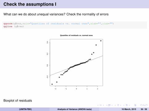
Check the assumptions I

What can we do about unequal variances? Check the normality of errors

qqnorm(g$res,main="Quantiles of residuals vs. normal ones",xlab="",ylab="")qqline (g$res)

●

●●

●

●

●

●

●

●●

●

●

●

●

●

●

●

●

●

●

●

●●

●

●

●

●

●

●

●

●

●

●

●●

●

●

●

●

●

●

●

●

●

●

●

●

●

−2 −1 0 1 2

−0.

20.

00.

20.

4

Quantiles of residuals vs. normal ones

Boxplot of residuals


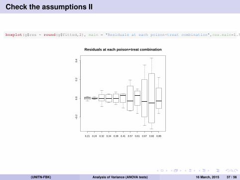
Check the assumptions II

boxplot(g$res ~ round(g$fitted,2), main = "Residuals at each poison+treat combination",cex.main=1.5) #look at box-plots of residuals

0.21 0.24 0.32 0.34 0.38 0.41 0.57 0.61 0.67 0.82 0.88

−0.

20.

00.

20.

4

Residuals at each poison+treat combination


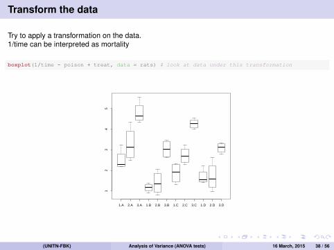
Transform the data

Try to apply a transformation on the data.1/time can be interpreted as mortality

boxplot(1/time ~ poison + treat, data = rats) # look at data under this transformation

1.A 2.A 3.A 1.B 2.B 3.B 1.C 2.C 3.C 1.D 2.D 3.D

12

34

5


Build the model on transformed data

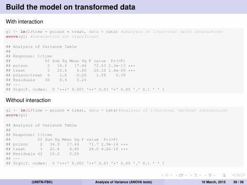
With interaction

g1 <- lm(1/time ~ poison * treat, data = rats) #analysis of 1/survival (with interaction)anova(g1) #interaction not significant

## Analysis of Variance Table#### Response: 1/time## Df Sum Sq Mean Sq F value Pr(>F)## poison 2 34.9 17.44 72.63 2.3e-13 ***## treat 3 20.4 6.80 28.34 1.4e-09 ***## poison:treat 6 1.6 0.26 1.09 0.39## Residuals 36 8.6 0.24## ---## Signif. codes: 0 '***' 0.001 '**' 0.01 '*' 0.05 '.' 0.1 ' ' 1

Without interaction

g1 <- lm(1/time ~ poison + treat, data = rats)#analysis of 1/survival (without interaction)anova(g1)

## Analysis of Variance Table#### Response: 1/time## Df Sum Sq Mean Sq F value Pr(>F)## poison 2 34.9 17.44 71.7 2.9e-14 ***## treat 3 20.4 6.80 28.0 4.2e-10 ***## Residuals 42 10.2 0.24## ---## Signif. codes: 0 '***' 0.001 '**' 0.01 '*' 0.05 '.' 0.1 ' ' 1


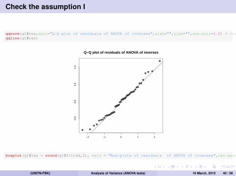
Check the assumption I

qqnorm(g1$res,main="Q-Q plot of residuals of ANOVA of inverses",xlab="",ylab="",cex.main=1.5) # visual test for the normality of residualsqqline(g1$res)

●

●●

●●

●

●

●

●

●

●

●

●

●

●

●

●

●

●

●

●

●

●

●

●

●

●

●

●

●

●

●

●

●

●

●

●

●

●

●

●

●

●

●

●

●

●

●

−2 −1 0 1 2

−0.

50.

00.

51.

0

Q−Q plot of residuals of ANOVA of inverses

boxplot(g1$res ~ round(g1$fitted,2), main = "Box-plots of residuals of ANOVA of inverses",cex.main=1.5) #boxplots


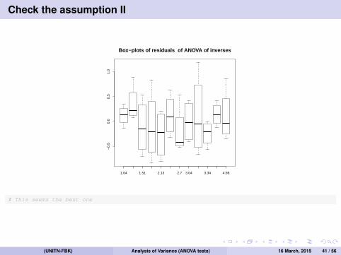
Check the assumption II

1.04 1.51 2.13 2.7 3.04 3.34 4.69

−0.

50.

00.

51.

0

Box−plots of residuals of ANOVA of inverses

# This seems the best one


ANOVASelect the right group

How to get the groups which differs?

1 Sort the means (m1 > m2 > ... > mN )2 Compare groups using t.test

NB correct for multiple testing

GN vs G1; GN vs G2 ...GN−1 vs G1 ......


Select the right group

Can we say anything aout the difference among treatments?Summary makes comparisons (via tests of single factor)It is not correct testing directly all possible differences thus there is an approximate procedure thatworks well (TukeyHSD)

TukeyHSD(aov(1/time ~ poison + treat, data = rats))

## Tukey multiple comparisons of means## 95% family-wise confidence level#### Fit: aov(formula = 1/time ~ poison + treat, data = rats)#### $poison## diff lwr upr p adj## 2-1 0.46864 0.045056 0.89223 0.02716## 3-1 1.99642 1.572839 2.42001 0.00000## 3-2 1.52778 1.104198 1.95137 0.00000#### $treat## diff lwr upr p adj## B-A -1.65740 -2.19593 -1.118870 0.00000## C-A -0.57214 -1.11067 -0.033604 0.03352## D-A -1.35834 -1.89687 -0.819806 0.00000## C-B 1.08527 0.54674 1.623799 0.00002## D-B 0.29906 -0.23947 0.837596 0.45509## D-C -0.78620 -1.32473 -0.247671 0.00184


Testing the variance

How do we check if the variances are homogeneous?

library(lawstat, quietly=TRUE)levene.test(1/rats$time, rats$treat, location="mean")

#### classical Levene's test based on the absolute deviations from the## mean ( none not applied because the location is not set to median## )#### data: 1/rats$time## Test Statistic = 0.9185, p-value = 0.4398

levene.test(rats$time, rats$treat, location="mean")

#### classical Levene's test based on the absolute deviations from the## mean ( none not applied because the location is not set to median## )#### data: rats$time## Test Statistic = 6.0747, p-value = 0.001494


Variable Selection

Select the “best” subset of predictors.

1 Simplest way to explain the data.Among several explanations for a phenomenon, the simplest is the best.

2 Unnecessary predictors will add noise to the estimation.Waste of degree of freedom.

3 Collinearity (too many variables doing the same job).4 Cost: computation time for complex models.


Stepwise ProcedureBackward Elimination and Forward Selection

Backward Elimination

1 Start with all the predictors in the model.2 Remove the predictor with highest p-value greater than αcrit .3 Refit the model and goto 24 Stop when all p-values are less than αcrit .

The αcrit is sometimes called the “p-to-remove” and does not have to be 5%. If predictionperformance is the goal, then a 15-20% cut-off may work best, although methods designed moredirectly for optimal prediction should be preferred.

∗ Forward Selection is the reverse of the backward elimination.


Stepwise ProcedureExamples

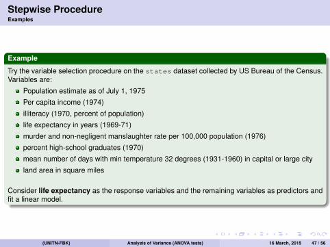
Example

Try the variable selection procedure on the states dataset collected by US Bureau of the Census.Variables are:

Population estimate as of July 1, 1975

Per capita income (1974)

illiteracy (1970, percent of population)

life expectancy in years (1969-71)

murder and non-negligent manslaughter rate per 100,000 population (1976)

percent high-school graduates (1970)

mean number of days with min temperature 32 degrees (1931-1960) in capital or large city

land area in square miles

Consider life expectancy as the response variables and the remaining variables as predictors andfit a linear model.



data(state)states <- data.frame(state.x77,row.names=state.abb)regtot <- lm(Life.Exp ~ .,data = states) # we do not need to write them all.## It's ok writing ~ . and this will use all variables but the response...summary(regtot)

#### Call:## lm(formula = Life.Exp ~ ., data = states)#### Residuals:## Min 1Q Median 3Q Max## -1.4890 -0.5123 -0.0275 0.5700 1.4945#### Coefficients:## Estimate Std. Error t value Pr(>|t|)## (Intercept) 7.09e+01 1.75e+00 40.59 < 2e-16 ***## Population 5.18e-05 2.92e-05 1.77 0.083 .## Income -2.18e-05 2.44e-04 -0.09 0.929## Illiteracy 3.38e-02 3.66e-01 0.09 0.927## Murder -3.01e-01 4.66e-02 -6.46 8.7e-08 ***## HS.Grad 4.89e-02 2.33e-02 2.10 0.042 *## Frost -5.74e-03 3.14e-03 -1.82 0.075 .## Area -7.38e-08 1.67e-06 -0.04 0.965## ---## Signif. codes: 0 '***' 0.001 '**' 0.01 '*' 0.05 '.' 0.1 ' ' 1#### Residual standard error: 0.745 on 42 degrees of freedom## Multiple R-squared: 0.736, Adjusted R-squared: 0.692## F-statistic: 16.7 on 7 and 42 DF, p-value: 2.53e-10



reg <- update(regtot, ~ . - Area) #take Area away from predictor variablessummary(reg)

#### Call:## lm(formula = Life.Exp ~ Population + Income + Illiteracy + Murder +## HS.Grad + Frost, data = states)#### Residuals:## Min 1Q Median 3Q Max## -1.4905 -0.5253 -0.0255 0.5716 1.5037#### Coefficients:## Estimate Std. Error t value Pr(>|t|)## (Intercept) 7.10e+01 1.39e+00 51.17 < 2e-16 ***## Population 5.19e-05 2.88e-05 1.80 0.079 .## Income -2.44e-05 2.34e-04 -0.10 0.917## Illiteracy 2.85e-02 3.42e-01 0.08 0.934## Murder -3.02e-01 4.33e-02 -6.96 1.5e-08 ***## HS.Grad 4.85e-02 2.07e-02 2.35 0.024 *## Frost -5.78e-03 2.97e-03 -1.94 0.058 .## ---## Signif. codes: 0 '***' 0.001 '**' 0.01 '*' 0.05 '.' 0.1 ' ' 1#### Residual standard error: 0.736 on 43 degrees of freedom## Multiple R-squared: 0.736, Adjusted R-squared: 0.699## F-statistic: 20 on 6 and 43 DF, p-value: 5.36e-11



Remove all the variables with high p-values.

reg <- update(regtot, ~ . - Illiteracy - Income - Area - Population)## remove all variables with high p-valuesummary(reg)$r.squared;summary(regtot)$r.squared

## [1] 0.71266## [1] 0.73616

summary(reg)$adj.r.squared;summary(regtot)$adj.r.squared

## [1] 0.69392## [1] 0.69218

NB: The R2 for the full model of 0.736 is reduced only slightly to 0.713 in the final model. Thus theremoval of four predictors causes only a minor reduction in fit. Beside, removing thePopulation variable could be a “close call” since the p-value is close to the αcrit of 5%.

We may want a more robust method to select the best variables.


Criterion-based procedures

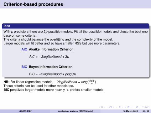
Idea

With p predictors there are 2p possible models. Fit all the possible models and chose the best onebase on some criteria.The criteria should balance the overfitting and the complexity of the model.Larger models will fit better and so have smaller RSS but use more parameters.

AIC Akaike Information Criterion

AIC = −2loglikelihood + 2p

BIC Bayes Information Criterion

BIC = −2loglikelihood + plog(n)

NB: For linear regression models, −2loglikelihood = nlog( RSSn )

These criteria can be used for other models too.BIC penalizes larger models more heavily -> prefers smaller models


Criterion-based proceduresExample

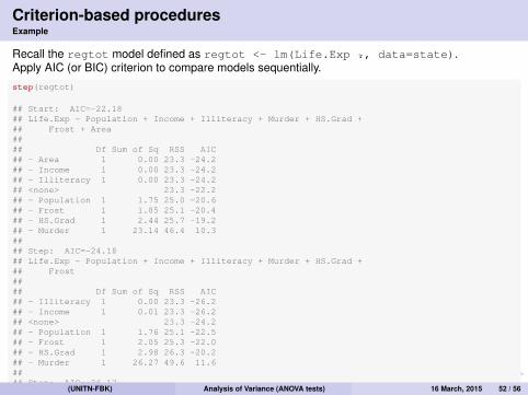
Recall the regtot model defined as regtot <- lm(Life.Exp ., data=state).Apply AIC (or BIC) criterion to compare models sequentially.

step(regtot)

## Start: AIC=-22.18## Life.Exp ~ Population + Income + Illiteracy + Murder + HS.Grad +## Frost + Area#### Df Sum of Sq RSS AIC## - Area 1 0.00 23.3 -24.2## - Income 1 0.00 23.3 -24.2## - Illiteracy 1 0.00 23.3 -24.2## <none> 23.3 -22.2## - Population 1 1.75 25.0 -20.6## - Frost 1 1.85 25.1 -20.4## - HS.Grad 1 2.44 25.7 -19.2## - Murder 1 23.14 46.4 10.3#### Step: AIC=-24.18## Life.Exp ~ Population + Income + Illiteracy + Murder + HS.Grad +## Frost#### Df Sum of Sq RSS AIC## - Illiteracy 1 0.00 23.3 -26.2## - Income 1 0.01 23.3 -26.2## <none> 23.3 -24.2## - Population 1 1.76 25.1 -22.5## - Frost 1 2.05 25.3 -22.0## - HS.Grad 1 2.98 26.3 -20.2## - Murder 1 26.27 49.6 11.6#### Step: AIC=-26.17## Life.Exp ~ Population + Income + Murder + HS.Grad + Frost#### Df Sum of Sq RSS AIC## - Income 1 0.0 23.3 -28.2## <none> 23.3 -26.2## - Population 1 1.9 25.2 -24.3## - Frost 1 3.0 26.3 -22.1## - HS.Grad 1 3.5 26.8 -21.2## - Murder 1 34.7 58.0 17.5#### Step: AIC=-28.16## Life.Exp ~ Population + Murder + HS.Grad + Frost#### Df Sum of Sq RSS AIC## <none> 23.3 -28.2## - Population 1 2.1 25.4 -25.9## - Frost 1 3.1 26.4 -23.9## - HS.Grad 1 5.1 28.4 -20.2## - Murder 1 34.8 58.1 15.5#### Call:## lm(formula = Life.Exp ~ Population + Murder + HS.Grad + Frost,## data = states)#### Coefficients:## (Intercept) Population Murder HS.Grad Frost## 7.10e+01 5.01e-05 -3.00e-01 4.66e-02 -5.94e-03


Adjusted R2

R2a = 1−

RSS/(n − p)TSS/(n − 1)

= 1−(n − 1

n − p

)(1− R2)

Adding a variable to a model can only decrease the RSS and so only increase the R2 so R2 byitself is not a good criterion because it would always choose the largest possible model.

Adding a predictor will only increase R2a if it has some value.

Recall R2:

R2 = 1−RSSTSS

= 1−∑

(yi − yi )2∑(yi − yi )2


Predicted residual sum of squares (PRESS)

RSS = ‖Y − Y‖2

may not represent adequately the predictive power of the model on other data.Predicted residual sum of squares (PRESS) is

n∑i=1

(yi − y(i))2

where y(i) is the value predicted for x = xi using the model on a dataset without the point xi , i.e.

β(i) = (X t(i)X(i))−1X t

(i)Y(i)

where the subscript (i) means that the i-th row and column have been deleted.It turns out

yi − y(i) =yi − yi

1− Hii.


Thesis topic at MPBA lab (FBK)

Data science theoretical projects

Deep Learningmathematical analysis applied on-omics or other big data.

Multiplex networksmathematical analysis and distanceanalysis and application on realdatasets.

Embedding network models inmachine learning for data integration.

Data science projectsIntegration and analysis of genetic dataand geographical information.

Project onhttp://opendata.unesco.orgdata. Prediction of expences andproject evaluation.

Energy consumption modelsmodulated by environmental factors.

Contact: [email protected]


http://opendata.unesco.org

[email protected]

Exercises

1 We would like to investigate the effectiveness of various feed supplements (feed) on thegrowth rate (weight) of chickens. Use boxplots and a plot of means to visualize thedifference between feed types. Use ANOVA to examine the effectiveness of feedsupplements. Comment on your findings and appropriateness of your assumptions.

2 We believe that mean urinary excretion rate of Pregnanetriol changes based on theunderlying type of Cushing’s syndrome. Investigate whether there is statistically significantmean difference for this steroid metabolites.

3 For the rat genotype data discussed during the lesson, use one-way ANOVA to investigatewhether weight gain (Wt) of the litter (in grams) at age 28 days is related to mother’s genotype(Mother). Repeat the analysis for the relationship between weight gain (Wt) and genotype ofthe litter (Litter). Compare the plot of means for the first analysis to that of the second one.

4 Load the anorexia data set from the MASS package. This data set was collected toinvestigate the effectiveness of different treatments (Treat) on increasing weight for youngfemale anorexia patients. Create a new variable called Difference by subtracting theweight of patient before study period (Prewt) from her weight after the study period(Postwt): Difference = Postwt - Prewt. Use a plot of means to visualize how thisvariable changes depending on the type of treatment. Use ANOVA to investigate whether thetype of treatment makes a difference in the amount of weight gain.

5 The data set cabbages available from the MASS package include a study on comparingascorbic acid content between two different cultivars of cabbage. In this data set, the twodifferent cultivars were planted on three different dates, denoted as d16, d20, or d21. Thevariable Data is a factor that specifies the planting date for each cabbage. Use two-wayANOVA to evaluate the relationship between the vitamin C content and cultivars whilecontrolling for the effect of planting dates.


Documents

Analysis of Variance (ANOVA tests) - unitn.it · Analysis of Variance (ANOVA tests) University of Trento - FBK 16 March, 2015 (UNITN-FBK) Analysis of Variance (ANOVA tests) 16 March,