Embed Size (px)
Citation preview

NASA/TM–2014–218280
Analysis of Well-Clear BoundaryModels for the Integration of UAS inthe NAS
Jason Upchurch, Cesar Munoz, Anthony Narkawicz,James Chamberlain, and Marıa ConsiglioLangley Research Center, Hampton, Virginia
June 2014

NASA STI Program . . . in Profile
Since its founding, NASA has been dedicatedto the advancement of aeronautics and spacescience. The NASA scientific and technicalinformation (STI) program plays a key partin helping NASA maintain this importantrole.
The NASA STI Program operates under theauspices of the Agency Chief InformationOfficer. It collects, organizes, provides forarchiving, and disseminates NASA’s STI.The NASA STI Program provides access tothe NASA Aeronautics and Space Databaseand its public interface, the NASA TechnicalReport Server, thus providing one of thelargest collection of aeronautical and spacescience STI in the world. Results arepublished in both non-NASA channels andby NASA in the NASA STI Report Series,which includes the following report types:
• TECHNICAL PUBLICATION. Reports ofcompleted research or a major significantphase of research that present the resultsof NASA programs and include extensivedata or theoretical analysis. Includescompilations of significant scientific andtechnical data and information deemed tobe of continuing reference value. NASAcounterpart of peer-reviewed formalprofessional papers, but having lessstringent limitations on manuscript lengthand extent of graphic presentations.
• TECHNICAL MEMORANDUM.Scientific and technical findings that arepreliminary or of specialized interest, e.g.,quick release reports, working papers, andbibliographies that contain minimalannotation. Does not contain extensiveanalysis.
• CONTRACTOR REPORT. Scientific andtechnical findings by NASA-sponsoredcontractors and grantees.
• CONFERENCE PUBLICATION.Collected papers from scientific andtechnical conferences, symposia, seminars,or other meetings sponsored orco-sponsored by NASA.
• SPECIAL PUBLICATION. Scientific,technical, or historical information fromNASA programs, projects, and missions,often concerned with subjects havingsubstantial public interest.
• TECHNICAL TRANSLATION. English-language translations of foreign scientificand technical material pertinent toNASA’s mission.
Specialized services also include creatingcustom thesauri, building customizeddatabases, and organizing and publishingresearch results.
For more information about the NASA STIProgram, see the following:
• Access the NASA STI program home pageat http://www.sti.nasa.gov
• E-mail your question via the Internet [email protected]
• Fax your question to the NASA STI HelpDesk at 443-757-5803
• Phone the NASA STI Help Desk at443-757-5802
• Write to:NASA STI Help DeskNASA Center for AeroSpace Information7115 Standard DriveHanover, MD 21076–1320

NASA/TM–2014–218280
Analysis of Well-Clear BoundaryModels for the Integration of UAS inthe NAS
Jason Upchurch, Cesar Munoz, Anthony Narkawicz,James Chamberlain, and Marıa ConsiglioLangley Research Center, Hampton, Virginia
National Aeronautics andSpace Administration
Langley Research CenterHampton, VA 23681-2199
June 2014

The use of trademarks or names of manufacturers in this report is for accurate reporting and does notconstitute an offical endorsement, either expressed or implied, of such products or manufacturers by theNational Aeronautics and Space Administration.
Available from:
NASA Center for AeroSpace Information7115 Standard Drive
Hanover, MD 21076-1320443-757-5802

Abstract
The FAA-sponsored Sense and Avoid Workshop for Unmanned Aircraft Systems(UAS) defines the concept of sense and avoid for remote pilots as “the capability ofa UAS to remain well clear from and avoid collisions with other airborne traffic.”Hence, a rigorous definition of well clear is fundamental to any separation assuranceconcept for the integration of UAS into civil airspace. This paper presents a familyof well-clear boundary models based on the TCAS II Resolution Advisory logic.Analytical techniques are used to study the properties and relationships satisfiedby the models. Some of these properties are numerically quantified using statisticalmethods.
iii

Acronyms
CAT Collision Avoidance ThresholdCDF Cumulative Distribution FunctionNAS National Airspace SystemNMAC Near Mid-Air CollisionRA Resolution AdvisorySAA Sense and AvoidSST Self-Separation ThresholdSSV Self-Separation VolumeTCAS Traffic Alerting and Collision Avoidance SystemTCPA Time to Closest Point of ApproachUAS Unmanned Aircraft Systems
1 Introduction
One of the major challenges of integrating Unmanned Aircraft Systems (UAS) intothe airspace system is the lack of an on-board pilot to comply with the legal re-quirement that pilots see and avoid other aircraft in their vicinity. To address thischallenge, the final report of the FAA-sponsored Sense and Avoid (SAA) Workshopfor Unmanned Aircraft Systems [2] defines the concept of sense and avoid for remoteUAS pilots as “the capability of a UAS to remain well clear from and avoid collisionswith other airborne traffic.” Under this definition, a rigorous definition of well clearbecomes fundamental to any sense and avoid concept that involves UAS.
NASA’s Unmanned Aircraft Systems Integration in the National Airspace Sys-tem (UAS in the NAS) project aims at conducting research towards the integrationof civil UAS into non-segregated airspace operations. As part of this project, NASAhas developed a sense and avoid concept for UAS that extends the concept out-lined by the SAA Workshop [1]. The NASA concept includes a volume, namely theSelf Separation Volume (SSV), located between the Collision Avoidance Threshold(CAT), defined by collision avoidance systems, and the Self-Separation Threshold(SST), defined by self-separation systems [2]. The SSV represents a well-clear bound-ary where aircraft inside the SSV are considered to be in well-clear violation. Thisvolume is intended to be large enough to avoid safety concerns for controllers andsee-and-avoid pilots, but small enough to avoid disruptions to traffic flow. A keycharacteristic of NASA’s concept is that the SSV is a conservative extension of theCAT defined by the Traffic Alerting and Collision Avoidance System (TCAS).
TCAS is a family of airborne devices that are designed to reduce the risk of mid-air collisions between aircraft equipped with operating transponders [10]. TCAS II,the current generation of TCAS devices, is mandated in the US for aircraft withgreater than 30 seats or a maximum takeoff weight greater than 33,000 pounds.Although it is not required, TCAS II is also installed on many turbine-poweredgeneral aviation aircraft. Version 7.0 is the current operationally-mandated versionof TCAS II, and Version 7.1 has been standardized [8]. In contrast to TCAS I, the

first generation of TCAS devices, TCAS II provides resolution advisories (RAs).RAs are visual and vocalized alerts that direct pilots to maintain or increase verticalseparation with intruders that are considered collision threats. TCAS II resolutionadvisories can be corrective or preventive depending on whether the pilot is expectedto change or maintain the aircraft’s current vertical speed. Corrective RAs areparticularly disruptive to the air traffic system since they may cause drastic evasivemaneuvers. For this reason, they are intended as a last resort maneuver when allother means of separation have failed.
The core of the TCAS II RA logic is a test that checks distance and time variablesfor the horizontal and vertical dimensions against a set of pre-defined thresholdvalues. To ensure interoperability between NASA’s SAA concept and TCAS, themathematical definition of the volume SSV is based on the TCAS II ResolutionAdvisory Logic [5]. The definition of SSV follows the same logic, but uses differentthresholds that conservatively extends the collision avoidance threshold providedby TCAS. This paper further generalizes the definition of the well-clear violationvolume presented in [5] and presents a family of mathematical well-clear boundarymodels that are all based on the TCAS II RA logic. Formal and statistical techniquesare used to study properties of this family of models.
The formal development presented in this paper is part of the NASA’s Air-borne Coordinated Resolution and Detection (ACCoRD) mathematical framework,which is electronically available from http://shemesh.larc.nasa.gov/people/
cam/ACCoRD. All theorems in this paper have been formally verified in the Pro-totype Verification System (PVS) [7], an automated theorem prover.
2 Distance and Time Variables
Distance and time variables are important elements of any separation assuranceconcept. These variables are functions over the aircraft current states which arecompared against distance and time thresholds. Many conflict detection and res-olution systems rely on the time of closest point of approach and the distance atthat time as their main time and distance variables [4]. This section describes someadditional distance and time variables that are particularly relevant to the definitionof a well-clear boundary model.
This paper assumes that accurate aircraft surveillance information is availableas horizontal and vertical components in a three-dimensional (3-D) airspace. Let-ters in bold-face denote two-dimensional (2-D) vectors. Vector operations such asaddition, subtraction, scalar multiplication, dot product, i.e., s · v ≡ sxvx + syvy,
the square of a vector, i.e., s2 ≡ s · s, and the norm of a vector, i.e., ‖s‖ ≡√
s2,are defined in a 2-D Euclidean geometry. Furthermore, the expression v⊥ denotes aparticular 2-D right-perpendicular vector of v, i.e., v⊥ ≡ (vy,−vx), and 0 denotesthe 2-D vector whose components are 0, i.e., 0 ≡ (0, 0).
The mathematical models presented in this paper consider two aircraft referredto as the ownship and the intruder aircraft. For the ownship, the current horizontalposition and velocity are denoted so and vo, respectively. Its altitude and verticalspeed are denoted soz and voz, respectively. Similarly, the horizontal position and
2

velocity of the intruder aircraft are denoted si and vi, respectively, and its verti-cal altitude and speed are denoted siz and viz, respectively. As it simplifies themathematical development, this paper uses a relative coordinate system where theintruder is static at the center of the coordinate system. In this relative system,s = so− si and v = vo−vi represent the horizontal relative position and velocity ofthe aircraft, respectively. Furthermore, sz = soz − siz and vz = voz − viz representthe vertical relative position and speed of the aircraft, respectively.
Assuming constant relative horizontal velocity v, the horizontal range betweenthe aircraft at any time t is given by
r(t) ≡ ‖s + tv‖ =√
s2 + 2t(s · v) + t2v2. (1)
The time of horizontal closest point of approach, denoted tcpa, is the time t thatsatisfies r(t) = 0, i.e., t = − s·v
v2 . The dot product s · v characterizes whether theaircraft are horizontally diverging, i.e., s · v > 0, or horizontally converging, i.e.,s · v < 0. By convention, tcpa is defined as 0 when v = 0. Hence, tcpa is formallydefined as
tcpa(s,v) ≡
{− s·v
v2 if v 6= 0,
0 otherwise.(2)
It is noted that tcpa(s,v) > 0 when the aircraft are horizontally converging, tcpa(s,v) <0 when the aircraft are horizontally diverging, and tcpa(s,v) = 0 when the aircraftare neither converging or diverging. The distance at time of closest point of approachis defined as
dcpa(s,v) ≡ r(tcpa(s,v)) = ‖s + tcpa(s,v)v‖. (3)
In the vertical dimension, assuming constant relative vertical speed, the relativealtitude between the aircraft at any time t is given by
rz(t) ≡ |sz + tvz|. (4)
The time to co-altitude tcoa is the time t that satisfies rz(t) = 0, i.e, t = − szvz
.Similar to the horizontal case, the product szvz characterizes whether the aircraftare vertically diverging, i.e., szvz > 0, or vertically converging, i.e., szvz < 0.This paper defines time to co-altitude as −1 when the aircraft are not verticallyconverging. Therefore,
tcoa(sz, vz) ≡
{− szvz
if szvz < 0,
−1 otherwise.(5)
Formula (5) is well defined since szvz < 0 implies that vz 6= 0.
2.1 Horizontal Time Variables
A (horizontal) time variable is a function that maps a relative horizontal positionand velocity into a real number. This real number is negative when the aircraftare horizontally diverging. When the real number is non-negative, this numberrepresents a time that, in a separation assurance logic, is intended to be compared
3

against a time threshold. In this paper, the time threshold is called TTHR. Anexample of a time variable that is used in conflict detection logics is tcpa [4].
The time variable used in earlier versions of the TCAS detection logic is calledtau, denoted τ [8]. Tau estimates tcpa, but is less demanding on sensor and surveil-lance technology than tcpa. Indeed, τ is simply defined as range over closure rate,
where closure rate is the negative of the range rate, i.e., τ = − r(0)r(0) = − ‖s‖s·v
‖s‖= − s2
s·v .
This paper defines τ as −1 when the aircraft are not horizontally converging. For-mally,
τ(s,v) ≡
{− s2
s·v if s · v < 0,
−1 otherwise.(6)
For a limited number of scenarios, the values of τ and tcpa coincide. However, inmost scenarios, the value of τ tends toward infinity as the aircraft approach theclosest point of approach. In general, τ is a good approximation of tcpa, but only forlarge values. For that reason, TCAS II uses a modified variant of τ called modifiedtau, denoted τmod [8]. Modified tau provides a better estimation of tcpa and has amore desirable behavior than τ in the proximity of the closest point of approach.
In [3], modified tau is defined such that τmod = − r(0)2−DTHR2r(0) = DTHR2−s2
s·v . Similar toτ , τmod is defined as -1 when the aircraft are not horizontally converging, i.e.,
τmod(s,v) ≡
{DTHR2−s2
s·v if s · v < 0,
−1 otherwise.(7)
The definition of τmod in Formula (7) depends on DTHR, which is a horizontal distancethreshold. This threshold is called DMOD in the TCAS II RA logic, and its actualvalue depends on a sensitivity level based on the ownship’s altitude [8].
In [6], a time variable called time to entry point, denoted tep, is proposed. Timeto entry point is defined as the time to loss of horizontal separation with respectto DTHR assuming straight-line aircraft trajectories. Similar to tcpa, tep decreaseslinearly over time. Time to entry point is formally defined as
tep(s,v) ≡
{Θ(s,v, DTHR,−1) if s · v < 0 and ∆(s,v, DTHR) ≥ 0,
−1 otherwise,(8)
where
Θ(s,v, D, ε) ≡−s · v + ε
√∆(s,v, D)
v2, (9)
∆(s,v, D) ≡ D2v2 − (s · v⊥)2. (10)
The function Θ is only defined when v 6= 0 and ∆(s,v, D) ≥ 0. In this case, itcomputes the times when the aircraft will lose separation, if ε = −1, or regainseparation, if ε = 1, with respect to D. When the aircraft are not horizontallyconverging or ∆(s,v, D) < 0, time to entry point is defined as -1. Formula (8) iswell defined since the condition s · v < 0 guarantees that v 6= 0.
4

2.2 Properties of Horizontal Time Variables
A useful property of a time variable is symmetry. A time variable tvar is said to besymmetric if and only for all s,v,
tvar(s,v) = tvar(−s,−v). (11)
Symmetry guarantees that in a pairwise scenario both the ownship and intruderaircraft compute the same value for the time variable. Hence, checking a symmetrictime variable against a given time threshold returns the same Boolean value for bothaircraft.
Theorem 1. The time variables τ , tcpa, τmod, and tep are symmetric.
It is possible to define time variables that are not symmetric. For instance,a time variable that computes the first time when the intruder aircraft enters anelliptical area aligned to the ownship trajectory is not symmetric for every scenario.However, any time variable can be transformed into a symmetric one by using minand max operators. For instance, the time variables min(tvar(s,v), tvar(−s,−v)) andmax(tvar(s,v), tvar(−s,−v)) are symmetric for any time variable tvar.
Figure 1 shows a graph of τ , tep, τmod, and tcpa versus time for an initial scenariowhere the ownship and intruder aircraft are located at (0 nmi,−3.25 nmi) and(−6.25 nmi, 0.25 nmi), respectively, flying at co-altitude. Furthermore, the ownshipground speed is 150 kn, heading 53o, and the intruder ground speed is 350 kn,heading 90o.1 In this scenario, the distance threshold DTHR used in the definition ofτmod and tep is 1 nmi. This scenario illustrates that while tep, τmod, and tcpa decreaseover time, the time variable τ decreases up to some point, but then it abruptlyincreases in the vicinity of the closest point of approach. Moreover, when these timevariables are checked against a time threshold TTHR, represented by the horizontalline at 30 seconds, the time variable tep crosses the time threshold first, followedby τmod, then tcpa, and finally τ . Interestingly, this ordering property holds for anyconverging scenario and any choice of common threshold values.
Theorem 2. Let s,v be such that s · v < 0, ‖s‖ > DTHR, and dcpa(s,v) ≤ DTHR,i.e., the aircraft are horizontally converging, are outside the distance threshold DTHR,and their distance at time of closest point of approach is less than or equal to DTHR.Then the following inequalities hold
tep(s,v) ≤ τmod(s,v) ≤ tcpa(s,v) ≤ τ(s,v). (12)
3 A Family of Well-Clear Boundary Models
A well-clear boundary specifies the set of aircraft states that are considered to bein well-clear violation. Following the TCAS detection logic, the well-clear boundarymodels in this paper are specified by a logical condition that simultaneously checks
1Aircraft headings are measured in true north clockwise convention, i.e., 0o points to the northand degrees are positive in clockwise direction.
5

0 10 20 30 40 50 60 70 80 90 1000
10
20
30
40
50
60
70
80
90
100
time (s)
tim
e (
s)
‖vo‖ =150 kn
track vo =53◦
‖vi‖ =350 kn
track vi =90◦
τ
tcp aτmodtepTTHR
Figure 1: Time vs. τ , tcpa, τmod, tep
horizontal and vertical violations. A horizontal violation occurs if the current rangeis less than a given horizontal distance threshold DTHR. A horizontal violation alsooccurs if distance at time of closest point of approach is less than DTHR and a giventime variable tvar is less than a given time threshold TTHR. In the vertical dimension,a similar comparison is made. Vertical well clear is violated if the relative altitudeis less than a given altitude threshold ZTHR or if the time to co-altitude is lessthan a given vertical time threshold TCOA. The distance and altitude thresholds areconsidered to be positive numbers, i.e., DTHR > 0 and ZTHR > 0. The time thresholdsare considered to be non-negative, i.e., TTHR ≥ 0 and TCOA ≥ 0. Formally, this well-clear violation condition can be denoted as follows.
WCVtvar(s, sz,v, vz) ≡ Horizontal WCVtvar(s,v) and
Vertical WCV(sz, vz),(13)
where
Horizontal WCVtvar(s,v) ≡ ‖s‖ ≤ DTHR or
(dcpa(s,v) ≤ DTHR and 0 ≤ tvar(s,v) ≤ TTHR),
Vertical WCV(sz, vz) ≡ |sz| ≤ ZTHR or 0 ≤ tcoa(sz, vz) ≤ TCOA.
The logical condition WCVtvar defines a family of well-clear boundary modelswhere tvar can be instantiated with any time variable, and DTHR, TTHR, ZTHR, andTCOA are set to threshold values of interest. The fact that the time thresholds TTHRand TCOA can be zero allows for the definition of well-clear boundary models thatdo not depend on time thresholds. For instance, when TTHR = 0 and TCOA = 0,WCVtcpa specifies the loss of separation condition for a cylindrical volume of radius
6

DTHR and half-height ZTHR around one of the aircraft. Indeed, in this case, WCVtcpa
is logically equivalent to the logical condition ‖s‖ ≤ DTHR and |sz| ≤ ZTHR.
The TCAS II RA core logic provided in [5] is used by WCVτmod, where DTHR,
TTHR, ZTHR, and TCOA are set to the TCAS II thresholds DMOD, TAU, ZTHR, andTAU, respectively. The actual values of these thresholds are given in a table indexedby sensitivity levels based on the ownship’s altitude [8]. In the TCAS II RA logic,the logical condition dcpa(s,v) ≤ DTHR in the horizontal check is called horizontalmiss-distance filter and, in that condition, DTHR is set to the miss-horizontal distancethreshold HMD, which is equal to DMOD. The well-clear boundary model definedin [6] is obtained by WCVtep , where TCOA = TTHR.
Henceforth, the well-clear models specified by WCVτ , WCVtcpa , WCVτmod, and
WCVtep will be referred to as WC TAU, WC TCPA, WC TAUMOD, and WC TEP,respectively. The rest of this section studies properties and relations satisfied bythese models.
3.1 Symmetry
A well-clear boundary model specified by WCVtvar , for a given time variable tvar, issymmetric if and only if
WCVtvar(s, sz,v, vz) = WCVtvar(−s,−sz,−v,−vz). (14)
In other words, in a symmetric well-clear boundary model, both the ownship andintruder aircraft have the same perception of being well clear or not.
Theorem 3 (Symmetry). If tvar is symmetric, the well-clear boundary model speci-fied by WCVtvar is symmetric. Hence, by Theorem 1, the well-clear boundary modelsWC TAU, WC TCPA, WC TAUMOD, and WC TEP are symmetric for any choiceof threshold values DTHR, TTHR, ZTHR, and TCOA.
3.2 Inclusion
Figure 2 illustrates the violation areas for the well-clear boundary models WC TAU,WC TAUMOD, WC TCPA, and WC TEP for the scenario of Figure 1. The thresh-old values used in this scenario are DTHR = 1 nmi, TTHR = TCOA = 30 s, andZTHR = 475 ft. The violation areas in these figures are similar to the conflict con-tours proposed in [9]. The points in these areas represent future locations of theownship where a well-clear violation will occur assuming that the intruder aircraftcontinues its current trajectory and the ownship either continues its current trajec-tory or instantaneously changes its direction but keeps its ground speed.
Figure 3 overlays the violation areas for the four boundary models. This figureillustrates that for a common set of threshold values, the violation area of WC TAUis included in the violation area of WC TCPA, which is included in the violation areaof WC TAUMOD, which is included in the violation area of WC TEP. Theorem 4below states that this inclusion property always holds for any encounter geometryand choice of common threshold values. Theorem 4 is a consequence of Theorem 2.
7

−7 −6 −5 −4 −3 −2 −1 0 1 2 3 4−6
−5
−4
−3
−2
−1
0
1
so = (0.00 nmi, −3.25 nmi)
vo = (119.8 kn, 90.3 kn)
si = (−6.25 nmi, 0.25 nmi)
vi = (350.0 kn, 0.0 kn)
x (nmi)
y (
nm
i)
WC_TAU
Area = 4.8 nmi2
Time to Violation = 84 sViolation Duration = 10 s
Ownship
Intruder
−7 −6 −5 −4 −3 −2 −1 0 1 2 3 4−6
−5
−4
−3
−2
−1
0
1
so = (0.00 nmi, −3.25 nmi)
vo = (119.8 kn, 90.3 kn)
si = (−6.25 nmi, 0.25 nmi)
vi = (350.0 kn, 0.0 kn)
x (nmi)
y (
nm
i)
WC_TCPA
Area = 5.1 nmi2
Time to Violation = 73 sViolation Duration = 32 s
Ownship
Intruder
(a) WC TAU (b) WC TCPA
−7 −6 −5 −4 −3 −2 −1 0 1 2 3 4−6
−5
−4
−3
−2
−1
0
1
so = (0.00 nmi, −3.25 nmi)
vo = (119.8 kn, 90.3 kn)
si = (−6.25 nmi, 0.25 nmi)
vi = (350.0 kn, 0.0 kn)
x (nmi)
y (
nm
i)
WC_TAUMOD
Area = 5.3 nmi2
Time to Violation = 73 sViolation Duration = 32 s
Ownship
Intruder
−7 −6 −5 −4 −3 −2 −1 0 1 2 3 4−6
−5
−4
−3
−2
−1
0
1
so = (0.00 nmi, −3.25 nmi)
vo = (119.8 kn, 90.3 kn)
si = (−6.25 nmi, 0.25 nmi)
vi = (350.0 kn, 0.0 kn)
x (nmi)
y (
nm
i)
WC_TEP
Area = 5.8 nmi2
Time to Violation = 71 sViolation Duration = 34 s
Ownship
Intruder
(c) WC TAUMOD (d) WC TEP
Figure 2: Violation areas for scenario of Figure 1
−7 −6 −5 −4 −3 −2 −1 0 1 2 3 4−6
−5
−4
−3
−2
−1
0
1
so = (0.00 nmi, −3.25 nmi)
vo = (119.8 kn, 90.3 kn)
si = (−6.25 nmi, 0.25 nmi)
vi = (350.0 kn, 0.0 kn)
x (nmi)
y (
nm
i)
WC_TAU
WC_TCPA
WC_TAUMOD
WC_TEP
Figure 3: Overlay of violation areas for scenario of Figure 1
8
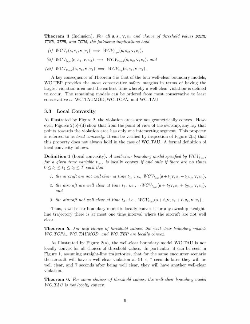
Theorem 4 (Inclusion). For all s, sz,v, vz and choice of threshold values DTHR,TTHR, ZTHR, and TCOA, the following implications hold
(i) WCVτ (s, sz,v, vz) =⇒ WCVtcpa(s, sz,v, vz),
(ii) WCVtcpa(s, sz,v, vz) =⇒ WCVτmod(s, sz,v, vz), and
(iii) WCVτmod(s, sz,v, vz) =⇒ WCVtep(s, sz,v, vz).
A key consequence of Theorem 4 is that of the four well-clear boundary models,WC TEP provides the most conservative safety margins in terms of having thelargest violation area and the earliest time whereby a well-clear violation is definedto occur. The remaining models can be ordered from most conservative to leastconservative as WC TAUMOD,WC TCPA, and WC TAU.
3.3 Local Convexity
As illustrated by Figure 2, the violation areas are not geometrically convex. How-ever, Figures 2(b)-(d) show that from the point of view of the ownship, any ray thatpoints towards the violation area has only one intersecting segment. This propertyis referred to as local convexity. It can be verified by inspection of Figure 2(a) thatthis property does not always hold in the case of WC TAU. A formal definition oflocal convexity follows.
Definition 1 (Local convexity). A well-clear boundary model specified by WCVtvar,for a given time variable tvar, is locally convex if and only if there are no times0 ≤ t1 ≤ t2 ≤ t3 ≤ T such that
1. the aircraft are not well clear at time t1, i.e., WCVtvar(s+ t1v, sz+ t1vz,v, vz),
2. the aircraft are well clear at time t2, i.e., ¬WCVtvar(s + t2v, sz + t2vz,v, vz),and
3. the aircraft not well clear at time t3, i.e., WCVtvar(s + t3v, sz + t3vz,v, vz).
Thus, a well-clear boundary model is locally convex if for any ownship straight-line trajectory there is at most one time interval where the aircraft are not wellclear.
Theorem 5. For any choice of threshold values, the well-clear boundary modelsWC TCPA, WC TAUMOD, and WC TEP are locally convex.
As illustrated by Figure 2(a), the well-clear boundary model WC TAU is notlocally convex for all choices of threshold values. In particular, it can be seen inFigure 1, assuming straight-line trajectories, that for the same encounter scenariothe aircraft will have a well-clear violation at 91 s, 7 seconds later they will bewell clear, and 7 seconds after being well clear, they will have another well-clearviolation.
Theorem 6. For some choices of threshold values, the well-clear boundary modelWC TAU is not locally convex.
9
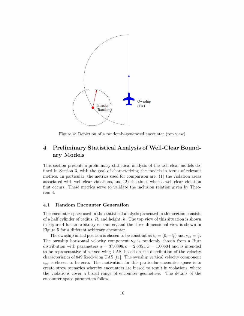
Figure 4: Depiction of a randomly-generated encounter (top view)
4 Preliminary Statistical Analysis of Well-Clear Bound-ary Models
This section presents a preliminary statistical analysis of the well-clear models de-fined in Section 3, with the goal of characterizing the models in terms of relevantmetrics. In particular, the metrics used for comparison are: (1) the violation areasassociated with well-clear violations, and (2) the times when a well-clear violationfirst occurs. These metrics serve to validate the inclusion relation given by Theo-rem 4.
4.1 Random Encounter Generation
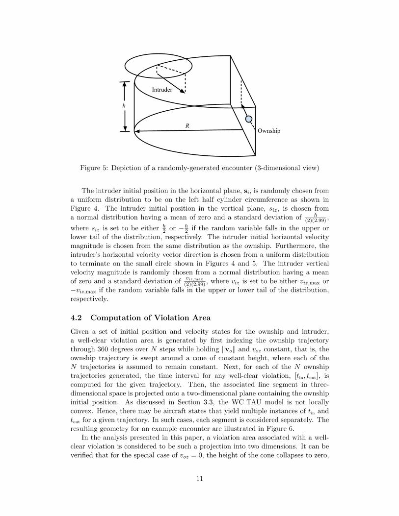
The encounter space used in the statistical analysis presented in this section consistsof a half cylinder of radius, R, and height, h. The top view of this situation is shownin Figure 4 for an arbitrary encounter, and the three-dimensional view is shown inFigure 5 for a different arbitrary encounter.
The ownship initial position is chosen to be constant as so = (0,−R2 ) and soz = h
2 .The ownship horizontal velocity component vo is randomly chosen from a Burrdistribution with parameters α = 37.0896, c = 2.6351, k = 1.00604 and is intendedto be representative of a fixed-wing UAS, based on the distribution of the velocitycharacteristics of 849 fixed-wing UAS [11]. The ownship vertical velocity componentvoz is chosen to be zero. The motivation for this particular encounter space is tocreate stress scenarios whereby encounters are biased to result in violations, wherethe violations cover a broad range of encounter geometries. The details of theencounter space parameters follow.
10
Intruder
Ownship
h
R
Figure 5: Depiction of a randomly-generated encounter (3-dimensional view)
The intruder initial position in the horizontal plane, si, is randomly chosen froma uniform distribution to be on the left half cylinder circumference as shown inFigure 4. The intruder initial position in the vertical plane, siz, is chosen froma normal distribution having a mean of zero and a standard deviation of h
(2)(2.99) ,
where siz is set to be either h2 or −h
2 if the random variable falls in the upper orlower tail of the distribution, respectively. The intruder initial horizontal velocitymagnitude is chosen from the same distribution as the ownship. Furthermore, theintruder’s horizontal velocity vector direction is chosen from a uniform distributionto terminate on the small circle shown in Figures 4 and 5. The intruder verticalvelocity magnitude is randomly chosen from a normal distribution having a meanof zero and a standard deviation of
viz,max
(2)(2.99) , where viz is set to be either viz,max or−viz,max if the random variable falls in the upper or lower tail of the distribution,respectively.
4.2 Computation of Violation Area
Given a set of initial position and velocity states for the ownship and intruder,a well-clear violation area is generated by first indexing the ownship trajectorythrough 360 degrees over N steps while holding ‖vo‖ and voz constant, that is, theownship trajectory is swept around a cone of constant height, where each of theN trajectories is assumed to remain constant. Next, for each of the N ownshiptrajectories generated, the time interval for any well-clear violation, [tin, tout], iscomputed for the given trajectory. Then, the associated line segment in three-dimensional space is projected onto a two-dimensional plane containing the ownshipinitial position. As discussed in Section 3.3, the WC TAU model is not locallyconvex. Hence, there may be aircraft states that yield multiple instances of tin andtout for a given trajectory. In such cases, each segment is considered separately. Theresulting geometry for an example encounter are illustrated in Figure 6.
In the analysis presented in this paper, a violation area associated with a well-clear violation is considered to be such a projection into two dimensions. It can beverified that for the special case of voz = 0, the height of the cone collapses to zero,
11

Figure 6: Projection of three-dimensional violation volume into two dimensions
and the original and projected volumes coincide.
The area of the two-dimensional violation area is computed as follows. First,consider a differential area in the polar coordinate system given by
dA =1
2(r2 − r2)dθ, (15)
where r corresponds to the distance from the ownship initial position to the positionat time tin, r corresponds to the distance from the ownship initial position to theposition at time tout, and dθ corresponds to the differential angle between adjacentownship trajectories, that is,
dθ =2π
N.
Thus, the analytical violation area is determined as
limN→∞
N∑k=1
M∑i=1
π
N(r2i,k − r2i,k), (16)
where M represents the number of violation regions on the kth trajectory, and ifa well-clear violation does not occur for the kth trajectory then ri,k and ri,k aredefined to be zero for that trajectory.
The algorithm implemented to compute the numerical approximation of theviolation area is given by
N∗∑k=1
∑i
π
N∗(r2i,k − r2j,k), (17)
12

0 20 40 60 80 100 120 1400
0.02
0.04
0.06
0.08
0.1
0.12
0.14
Number of part it ions (N )
P{
N||
Ai+
1−A
i|
|Ai+
1|≤
0.01}
Figure 7: Estimate of probability density function of N for 1000 trials
where N∗ denotes a particular choice for N . It can be verified that this estimateconverges to the actual area as N∗ approaches infinity.
The particular choice for N∗ used for the analysis in the remainder of this paperwas arrived at through a Monte Carlo experiment which was run until 1000 randomencounter trajectories resulting in well-clear violations were accumulated. For eachwell-clear violation, N was initialized with N = 2 and the corresponding violationarea was calculated using Formula (17). The value of N was then incremented byone and the violation area recomputed. This process continued until the relativedifference between the computed area and the previously-computed area was below1%. Thus, the value of N for any randomly-generated encounter was chosen asthe number of partitions that first satisfied the 1% condition. An estimate of thedistribution of N for the 1000 well-clear violations is shown in Figure 7. This figurewas used as a basis for choosing N∗ = 360, which is assumed for the remainderof the analysis in this paper. Thus, the differential angle for the velocity sweep isnecessarily 1◦.
4.3 Analysis
In the subsequent analysis, the choice is made to present comparisons of WC TAU,WC TCPA, and WC TAUMOD relative to WC TEP. That is, the analysis andmetrics presented are with respect to WC TEP. In particular, the two metricsused for the following discussion are: (1) the relative difference in violation areas,
13

determined as
∆A(tvar) =A(WCVtep)−A(WCVτ )
A(WCVtep), (18)
∆A(tvar) =A(WCVtep)−A(WCVtcpa)
A(WCVtep), (19)
∆A(tvar) =A(WCVtep)−A(WCVτmod
)
A(WCVtep), (20)
and (2) the difference in time when a well-clear violation will first occur, determinedas
∆tin(tvar) = tin(WCVtep)− tin(WCVτ ), (21)
∆tin(tvar) = tin(WCVtep)− tin(WCVtcpa), (22)
∆tin(tvar) = tin(WCVtep)− tin(WCVτmod). (23)
The statistical analysis of violation areas is obtained from a Monte Carlo sim-ulation with 10,000 well-clear violations (i.e., greater than 10,000 trials). Eachtrial consisted of a random encounter scenario having the geometry discussed inSection 4.1. For each trial, if the random encounter resulted in a joint well-clearviolation for all models, the corresponding areas were computed, followed by therelative area differences with respect to WC TEP. This process was repeated until10,000 joint well-clear violations were accumulated, and the cumulative distributionfunction (CDF) for WC TAUMOD and WC TCPA with respect to WC TEP wasthen computed (see Formulas 18-20). Figure 8 shows the results of the Monte Carloexperiment, where the threshold values used for the simulation were TTHR = 30 s,DTHR = 1 nmi, and ZTHR = 475 ft. The preliminary analysis of the CDFs in Figure 8reveal that: (1) the areas for WC TAUMOD and WC TEP differ by less than 25%in approximately 95% of the well-clear violations, (2) the areas for WC TCPA andWC TEP differ by as much as 55% in approximately 95% of the well-clear viola-tions, and (3) the areas for WC TAU and WC TEP differ by as much as 70% in95% of the well-clear violations. The Monte-Carlo results provide an experimentalvalidation of the inclusion property discussed in Section 3.2.
The second metric used to analyze the well-clear models is tin, the time when awell-clear violation first occurs (see Formulas 21-23). During the same Monte Carloexperiment previously discussed, if a joint well-clear violation for an initial set ofrandomly-generated ownship and intruder positions and velocities occurs, then thetime when the well-clear violation occurs for each model is computed using onlythe initial positions and velocities. For each encounter resulting in a well-clearviolation, the time difference with respect to WC TEP is computed for WC TAU,WC TCPA, and WC TAUMOD. Upon accumulation of 10,000 well-clear violations,the CDFs of the time difference in time were generated. The results of the MonteCarlo experiment are shown in Figure 9.
The CDFs in Figure 9 show that: (1) the difference between tin for WC TAUMODand WC TEP is limited to approximately 15 s, (2) the difference between tin for
14

0 0.1 0.2 0.3 0.4 0.5 0.6 0.7 0.8 0.9 10
0.1
0.2
0.3
0.4
0.5
0.6
0.7
0.8
0.9
1
δA(tvar) (relative difference)
P{δA(t
var)≤
∆A(t
var)|W
CVtvar}
∆A(τ )∆A(tcp a)∆A(τmod)
Figure 8: CDF of relative difference in area with respect to WC TEP
0 5 10 15 20 25 30 350
0.1
0.2
0.3
0.4
0.5
0.6
0.7
0.8
0.9
1
δt in(tvar) (s)
P{δtin(t
var)≤
∆tin(t
var)|W
CVtvar}
∆t in(τ )∆t in(tcp a)∆t in(τmod)
Figure 9: CFD of absolute difference first time to violation with respect to WC TEP
15

−2.5 −2 −1.5 −1 −0.5 0 0.5 1−1.6
−1.4
−1.2
−1
−0.8
−0.6
−0.4
−0.2
0
x (nmi)
y (
nm
i)
‖vo‖ =83.6 kts
track vo =0.0◦
‖v i‖ =126.8 kts
track v i =45.0◦
WC_TAU
WC_TCPA
WC_TAUMOD
WC_TEP
Figure 10: Encounter geometry of interest: large difference in tin
WC TCPA and WC TEP is limited to exactly 30 s, which is TTHR for the experi-ment, and (3) the difference between tin for WC TAU and WC TEP may slightlyexceed the 30-second TTHR.
While Figures 8 and 9 provide a visual validation of the inclusion property,additional insight can be gained by considering some examples designed to illustratethe implications of each particular well-clear model. Figures 10 and 11 show twosuch examples.
Figure 10 shows an encounter geometry designed to illustrate a case when all ofthe well-clear models indicate a well-clear violation will occur at some time in thefuture given the initial ownship and intruder trajectories, yet a significant differencein tin exists for each approach. In particular, the value for tin for each model is:
1. WC TAU 42 s,
2. WC TCPA 41.7 s,
3. WC TAUMOD 23.9 s,
4. WC TEP 11.7 s.
Thus, the maximum ∆tin is WC TEP−WC TAU = 30.3 s. This scenario depicts asituation where every model will eventually determine a well-clear violation existsfor the current, constant-velocity trajectory, however there is a wide range in tin,the time when such a violation first occurs. The figure also demonstrates anothercase of violation of the local convexity property for the WC TAU model.
16

−2.5 −2 −1.5 −1 −0.5 0 0.5−1.6
−1.5
−1.4
−1.3
−1.2
−1.1
−1
−0.9
−0.8
x (nmi)
y (
nm
i)
‖vo‖ =17.0 kts
track vo =135.0◦
‖v i‖ =92.7 kts
track v i =90.9◦
WC_TAU
WC_TCPA
WC_TAUMOD
WC_TEP
Figure 11: Encounter geometry of interest: non-agreement over WCVtvar
Figure 11 shows a case when all but one well-clear model results in a well-clearviolation for the initial trajectory. In particular, WC TCPA, WC TAUMOD, andWC TEP produce well-clear boundaries in any horizontal direction the ownship maytravel, however, the WC TAU model produces a region on the ownship’s currenttrajectory in which the ownship may pass without incurring a well-clear violation.This example was selected to illustrate that there are other important, characterizingproperties of the models appropriate for investigation beyond area and tin. Thispaper does not present an extensive analysis of such considerations.
5 Conclusion
A family of well-clear boundary models is presented. This family generalizes theTCAS II Resolution Logic with different possible definitions of horizontal time vari-ables including tau, time to closest point of approach, modified tau, and time toentry point. Analytical techniques are used to study the properties of this model.For instance, it has been formally proved that the well-clear model based on timeto entry point is more conservative than tau, time to closest point of approach, andmodified tau for any scenario and any common choice of threshold values. Further-more, it is shown that all the models in this family are symmetric, i.e., the ownshipand intruder aircraft have the same perception of being well-clear or not at anymoment in time. Except for the model based on tau, all the models are locallyconvex meaning that there is at most one interval of time when the aircraft are notwell-clear, assuming straight-line trajectories.
17

Some of these properties are validated through numerical quantification usingstatistical methods. In particular, random encounters are generated in Monte Carlofashion, and distributions for area and tin are determined for 10,000 data points.This analysis represents a preliminary look at some characterizing properties of thefamily of well-clear boundary models.
The mathematical development presented in this paper has been mechanicallyverified in the Prototype Verification System (PVS) [7]. This level of rigor is justifiedby the safety-critical nature of the well-clear concept to the integration of UnmannedAircraft Systems in the the National Aerospace System.
References
1. Marıa Consiglio, James Chamberlain, Cesar Munoz, and Keith Hoffler. Conceptof integration for UAS operations in the NAS. In Proceedings of 28th Interna-tional Congress of the Aeronautical Sciences, ICAS 2012, Brisbane, Australia,2012.
2. FAA Sponsored Sense and Avoid Workshop. Sense and avoid (SAA) for Un-manned Aircraft Systems (UAS), October 2009.
3. Jonathan Hammer. Horizontal miss distance filter system for suppressing falseresolution alerts, October 1996. U.S. Patent 5,566,074.
4. James Kuchar and Lee Yang. A review of conflict detection and resolutionmodeling methods. IEEE Transactions on Intelligent Transportation Systems,1(4):179–189, December 2000.
5. Cesar Munoz, Anthony Narkawicz, and James Chamberlain. A TCAS-II resolu-tion advisory detection algorithm. In Proceedings of the AIAA Guidance Nav-igation, and Control Conference and Exhibit 2013, AIAA-2013-4622, Boston,Massachusetts, 2013.
6. Anthony J. Narkawicz, Cesar A. Munoz, Jason M. Upchurch, James P. Cham-berlain, and Marıa C. Consiglio. A well-clear volume based on time to entrypoint. Technical Memorandum NASA/TM-2014-218155, NASA, Langley Re-search Center, Hampton VA 23681-2199, USA, January 2014.
7. S. Owre, J. Rushby, and N. Shankar. PVS: A prototype verification system. InDeepak Kapur, editor, Proc. 11th Int. Conf. on Automated Deduction, volume607 of Lecture Notes in Artificial Intelligence, pages 748–752. Springer-Verlag,June 1992.
8. RTCA SC-147. RTCA-DO-185B, Minimum operational performance standardsfor traffic alert and collision avoidance system II (TCAS II), July 2009.
9. J. Tadema, E. Theunissen, and K.M. Kirk. Self separation support for UAS. InAIAA Infotech@Aerospace 2010, number AIAA-2010-3460, Atlanta, GA, USA,April 2010.
18

10. U.S. Department of Transportation Federal Aviation Adminstration. Introduc-tion to TCAS II Version 7.1, February 2011.
11. Unmanned Vehicle Systems International (UVSI). RPAS: Remoted Piloted Air-craft Systems - The Global Perspective. Blyenburgh & Co., Paris, France, 10thedition, June 2012. uvs-info.com.
19

REPORT DOCUMENTATION PAGE Form ApprovedOMB No. 0704–0188
The public reporting burden for this collection of information is estimated to average 1 hour per response, including the time for reviewing instructions, searching existing data sources,gathering and maintaining the data needed, and completing and reviewing the collection of information. Send comments regarding this burden estimate or any other aspect of this collectionof information, including suggestions for reducing this burden, to Department of Defense, Washington Headquarters Services, Directorate for Information Operations and Reports(0704-0188), 1215 Jefferson Davis Highway, Suite 1204, Arlington, VA 22202-4302. Respondents should be aware that notwithstanding any other provision of law, no person shall besubject to any penalty for failing to comply with a collection of information if it does not display a currently valid OMB control number.PLEASE DO NOT RETURN YOUR FORM TO THE ABOVE ADDRESS.
Standard Form 298 (Rev. 8/98)Prescribed by ANSI Std. Z39.18
1. REPORT DATE (DD-MM-YYYY)01-06-2014
2. REPORT TYPE
Technical Memorandum3. DATES COVERED (From - To)
4. TITLE AND SUBTITLE
Analysis of Well-Clear Boundary Models for the Integration of UAS in theNAS
5a. CONTRACT NUMBER
5b. GRANT NUMBER
5c. PROGRAM ELEMENT NUMBER
5d. PROJECT NUMBER
5e. TASK NUMBER
5f. WORK UNIT NUMBER425425.04.01.07.02
6. AUTHOR(S)
Upchurch, Jason M.; Munoz, Cesar A.; Narkawicz, Anthony J.;Chamberlain, James P.; Consiglio, Maria C.
7. PERFORMING ORGANIZATION NAME(S) AND ADDRESS(ES)
NASA Langley Research CenterHampton, VA 23681-2199
8. PERFORMING ORGANIZATIONREPORT NUMBER
L–20407
9. SPONSORING/MONITORING AGENCY NAME(S) AND ADDRESS(ES)
National Aeronautics and Space AdministrationWashington, DC 20546-0001
10. SPONSOR/MONITOR’S ACRONYM(S)NASA
11. SPONSOR/MONITOR’S REPORTNUMBER(S)
NASA/TM–2014–218280
12. DISTRIBUTION/AVAILABILITY STATEMENT
Unclassified-UnlimitedSubject Category 03Availability: NASA CASI (443) 757-5802
13. SUPPLEMENTARY NOTES
An electronic version can be found at http://ntrs.nasa.gov.
14. ABSTRACT
The FAA-sponsored Sense and Avoid Workshop for Unmanned Aircraft Systems (UAS) defines the concept of sense andavoid for remote pilots as “the capability of a UAS to remain well clear from and avoid collisions with other airborne traffic.”Hence, a rigorous definition of well clear is fundamental to any separation assurance concept for the integration of UAS intocivil airspace. This paper presents a family of well-clear boundary models based on the TCAS II Resolution Advisory logic.Analytical techniques are used to study the properties and relationships satisfied by the models. Some of these properties arenumerically quantified using statistical methods.
15. SUBJECT TERMS
National airspace; Safety; Separation assurance; Unmanned aircraft systems; Well-Clear boundary; Well-Clear violation
16. SECURITY CLASSIFICATION OF:
a. REPORT
U
b. ABSTRACT
U
c. THIS PAGE
U
17. LIMITATION OFABSTRACT
UU
18. NUMBEROFPAGES
25
19a. NAME OF RESPONSIBLE PERSON
STI Help Desk (email: [email protected])
19b. TELEPHONE NUMBER (Include area code)
(443) 757-5802