Analytic and Nonlinear Prognostic for Vehicle Suspension Systems · cumulative damage theories. Ideally, the summation of life ratios would equal one at failure. However, past experiments

American Journal of Engineering and Applied Sciences, 6 (1): 42-56, 2013

ISSN: 1941-7020

© 2014 Jaoude and El-Tawil, This open access article is distributed under a Creative Commons Attribution

(CC-BY) 3.0 license

doi:10.3844/ajeassp.2013.42.56 Published Online 6 (1) 2013 (http://www.thescipub.com/ajeas.toc)

Corresponding Author: Abdo Abou Jaoude, Paul Cezanne University Aix-Marseille, France and the Lebanese University,

(EDST) Hadath, Lebanon

42 Science Publications

AJEAS

Analytic and Nonlinear

Prognostic for Vehicle Suspension Systems

1Abdo Abou Jaoude and

2Khaled El-Tawil

1Paul Cezanne University Aix-Marseille, France and the Lebanese University, (EDST) Hadath, Lebanon

2Faculty of Engineering and EDST, Lebanese University, Hadath, Lebanon

Received 2012-09-17, Revised 2012-12-27; Accepted 2013-04-23

ABSTRACT

Predicting Remaining Useful Lifetime (RUL) of industrial systems becomes currently an important aim for industrialists knowing that the expensive failure can occur suddenly. As the classical strategies of maintenance are not efficient and practical because they neglect the evolving product state and environment, the recent prognostic approaches try to fill this gap. This approach shows to be important in ensuring high availability in minimum costs for industrial systems, like in aerospace, defense, petro-chemistry and automobiles. An analytic prognostic methodology based on existing damage laws in fracture mechanics, such as Paris’ and Miner’s laws, is recently developed for determining the system RUL. Damages have been assumed to be accumulated linearly, since we have considered the widely used linear Miner’s law. In this study, the nonlinear case in damage accumulation is explored to take into account the complex behavior of some materials subject to fatigue effects. It is useful especially when the nature of applied constraints and influent environment contribute to accentuate this nonlinearity. Our damage model is based on the accumulation of a damage measurement D(N) after each loading cycle N. In automobile industry, the prognostic assessment of the suspension component by this developed nonlinear approach shows its importance for the same earlier reasons.

Keywords: Analytic Laws, Degradation, Fatigue, Miner’s Law, Paris’ Law, Nonlinear Cumulative

Damage, Prognostic

1. INTRODUCTION

It is well known that each system passes by three phases during its whole life. The last phase represents the degradation period of the system and which leads to failure by progressive deterioration. It is important for industrialists to predict, at each instant, the remaining lifetime in order to prevent expensive and unexpected failure. Early detection also helps in avoiding catastrophic failures. Adopting preventive systematic maintenance to increase the system availability proves to be an expensive strategy due to the frequent replacement of generally expensive accessories (Inman et al., 2005). Moreover, this strategy is not efficient because most of equipments failures are not related only to the number of hours of functioning. The prognostic (Vachtsevanos et al.,

2006) is a methodology that aims to predict the Remaining Useful Lifetime (RUL) of a system in service. RUL can be expressed in hours of functioning, in Kilometers run or in cycles. Lee (2004) defines prognostics as the ability to “predict and prevent” possible fault or system degradation before failures occur. Prognosis has been defined by (Lewis and Edwards, 1997) as “prediction of when a failure may occur” i.e., a mean to calculate remaining useful life of an asset. If we can effectively predict the condition of machines and systems, maintenance actions can be taken ahead of time. In order to make a good and reliable prognosis it must have good and reliable diagnosis.

An earlier prognostic work (Peysson, 2009) on

vehicle suspension system used an analytical model

based on degradation laws like Paris’ law for fatigue

Abdo Abou Jaoude and Khaled El-Tawil / American Journal of Engineering and Applied Sciences 6 (1): 42-56, 2013


AJEAS

degradation and Miner’s law for linear cumulative

fatigue damage. A degradation indicator D was taken to

describe the evolution from an initial micro-damage till

the total system failure.

Until now, damages have been assumed to accumulate linearly (Miner’s law) even though it is unlikely to be the case of brittle material. The present paper will explore the nonlinear side of cumulative damage to take into account the nature of the applied constraints and influent environment that can accentuate the nonlinear aspect related to some materials behavior subject to fatigue effects.

1.1. Nonlinear-Damage-based Prognostic: State

of the Art

Various approaches to prognostics have been

developed that range in fidelity from simple historical

failure rate models to high-fidelity physics-based models

(Byington et al., 2002). The required information

(depending on the type of prognostics approach) include:

engineering model and data, failure history, past

operating conditions, current conditions, identified fault

patterns, transitional failure trajectories, maintenance

history, system degradation and failure modes.

A number of different methods have been applied to study prognosis of degraded components. In general, prognostics approaches can be classified into three primary categories: (1) model driven, (2) data driven and (3) probability based prognostic techniques.

The main advantage of model based approaches is their ability to incorporate physical understanding of the monitored system (Luo et al., 2003). Moreover, if the understanding of the system degradation improves, the model can be adapted to increase its accuracy and to address subtle performance problems. Consequently,

they can significantly outperform data-driven approaches. But, this closed relation with a mathematical model may also be a strong weakness: It can be difficult, even impossible to catch the system’s behavior. Furthermore, some authors think that the monitoring and prognostic tools must evolve as the system does. An earlier proposed procedure (Abou Jaoude et al.,

2010) belongs to the first prognostic approach and is

based on a physical model leading to a degradation

indicator. It is focused on developing and implementing

effective diagnostic and prognostic technologies with the

ability to detect faults in the early stages of degradation.

Early detection and analysis may lead to better prediction

and end of life estimates by tracking and modeling the

degradation process. The idea was to use these estimates

to make accurate and precise prediction of the time to

failure of components. The case of fatigue degradation

chosen is mathematically formulated by analytic laws

such as Paris and Miner laws. The last law is a linear

cumulative damage model.

Past research has shown there is a nonlinear

interaction effect between High Cycle Fatigue (HCF)

and Low Cycle Fatigue (LCF) in many engineering

materials. This effect has been observed within uniaxial

loadings, but is often more pronounced under multiaxial

loading, particularly when the loading is non-

proportional. An example here is the development of

fatigue damage assessment methods for turbine engine

materials combining the LCF and HCF cycles.

The nonlinear interaction effect precludes the use of

the most common technique for damage accumulation,

the Palmgren-Miner linear damage rule. A thorough

review of nonlinear cumulative damage methodologies

(Goodin et al., 2007) shows that these techniques have

included simple extensions of the linear damage rule to

include nonlinear terms. Several nonlinear methods exist,

including endurance-limit modification techniques,

fracture-mechanics based approaches, continuum-

damage and life-curve approaches. Traditional methods

of damage summation have been shown to provide an

inaccurate life prediction when multiple load levels are

simultaneously considered. This is due to the effect that

one load level has on the other (s).

In the present study, the effect of HCF loading has had a more detrimental effect when coupled with the LCF loadings than predicted by a linear summation rule. Nonlinear damage accumulation theories can account for this influence and have shown an improvement in prediction. The stress levels were chosen to correspond

to levels previously tested to failure, resulting in fatigue lives ranging from approximately 10

5 to 10

7 cycles. A

nonlinear damage summation is required to properly define the fatigue process since the linear summation of damage (Miner’s sum) is often not adequate to predict the service life of a component when subjected to

variable-amplitude loadings.

1.2. Linear Damage Rule

The most common method of summing damage for

a loading spectrum is the Miner’s rule (Miner, 1945). It

is readily understood and easy to implement and is,

therefore, the foundation for many of the other proposed

cumulative damage theories. Ideally, the summation of

life ratios would equal one at failure. However, past

experiments have yielded a range of ratios from 0.7 to

2.2 for uniaxial loadings, resulting in failure predictions

erring just slightly on the side of non-conservative to



AJEAS

more than the double for a conservative prediction

(Shigley and Mischke, 1989). For the biaxial loadings, a

Miner’s summation of 0.19 was found indicating

extremely non-conservative results.

The largest drawback of the linear damage rule is its

inability to account for the order of loading. That is, the

resulting failure prediction is independent of the load

interaction effects that have been observed between

high-cycle and low-cycle loadings. It is this shortcoming

that has prompted the development of several nonlinear

cumulative damage theories.

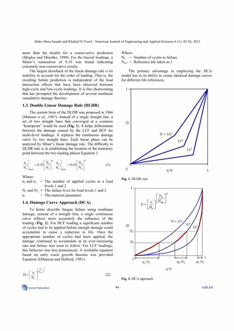
1.3. Double Linear Damage Rule (DLDR)

The current form of the DLDR was proposed in 1966

(Manson et al., 1967). Instead of a single straight line, a

set of two straight lines that converged at a common

“Kneepoint” would be used (Fig. 1). It helps differentiate

between the damage caused by the LCF and HCF for

multi-level loadings. It replaces the continuous damage

curve by two straight lines. Each linear phase can be

analyzed by Miner’s linear damage rule. The difficulty in

DLDR rule is in establishing the location of the transitory

point between the two loading phases Equation 1:

1 1 2 1

1 2 2 2knee knee

n N n N0.35 0.65

N N N N

α α

= =

(1)

Where:

n1 and n2 = The number of applied cycles at a load

levels 1 and 2

N1 and N2 = The failure lives for load levels 1 and 2

α = The material parameter

1.4. Damage Curve Approach (DCA)

To better describe fatigue failure using nonlinear

damage, instead of a straight line, a single continuous

curve reflects more accurately the influence of the

loading (Fig. 2). For HCF loading a significant number

of cycles had to be applied before enough damage could

accumulate to cause a reduction in life. Once the

appropriate number of cycles had been applied, the

damage continued to accumulate at an ever-increasing

rate and failure was soon to follow. For LCF loadings,

this behavior was less pronounced. A workable equation

based on early crack growth theories was provided

Equation 2(Manson and Halford, 1981):

f

ref

N

N

f

nD

N

α

=

(2)

Where:

Nf = Number of cycles to failure

Nref = Reference life taken as 1

The primary advantage in employing the DCA

model lies in its ability to create identical damage curves

for different life references.

Fig. 1. DLDR rule

Fig. 2. DCA approach



AJEAS

The linear damage line becomes the reference life that is

used to establish the material constant in the Equation 2

above and other damage curves shift values accordingly.

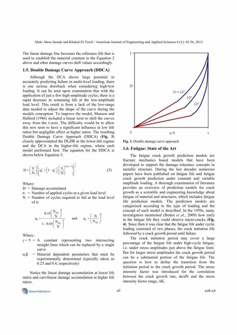
1.5. Double Damage Curve Approach (DDCA)

Although the DCA shows large potential in

accurately predicting failure in multi-level loading, there

is one serious drawback when considering high-low

loading. It can be seen upon examination that with the

application of just a few high-amplitude cycles, there is a

rapid decrease in remaining life at the low-amplitude

load level. This result is from a lack of the low-range

data needed to adjust the shape of the curve during the

models conception. To improve the model, Manson and

Halford (1986) included a linear term to shift the curves

away from the x-axis. The difficulty would be to allow

this new term to have a significant influence at low life

ratios but negligible effect at higher ratios. The resulting

Double Damage Curve Approach (DDCA) (Fig. 3)

closely approximated the DLDR in the lower-life regime

and the DCA in the higher-life regime, where each

model performed best. The equation for the DDCA is

shown below Equation 3:

( )2

1

q 1

1 1

n nD . q 1 q .

N N

γ − γγγ

= + − (3)

Where:

D = Damage accumulated

n = Number of applied cycles at a given load level

N = Number of cycles required to fail at the load level

of n:

1 2

ref

refref

N0.35

NNq and q

NN1 0.65

N

α

β

α

= = −

Where:

γ = 5 = A constant representing two intersecting

straight lines which can be replaced by a single

curve

α,β = Material dependent parameters that must be

experimentally determined (typically taken as

0.25 and 0.4, respectively)

Notice the linear damage accumulation at lower life

ratios and curvilinear damage accumulation at higher life

ratios.

Fig. 3. Double damage curve approach

1.6. Fatigue: State of the Art

The fatigue crack growth prediction models are

fracture mechanics based models that have been

developed to support the damage tolerance concepts in

metallic structure. During the last decades numerous

papers have been published on fatigue life and fatigue

crack growth prediction under constant and variable

amplitude loading. A thorough examination of literature

provides an overview of prediction models for crack

growth as a scientific and engineering knowledge about

fatigue of material and structures, which includes fatigue

life prediction models. The prediction models are

categorized according to the type of loading and the

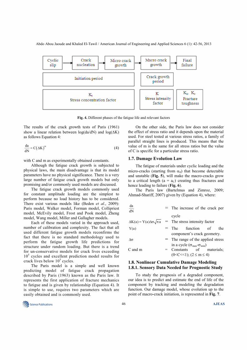
concept of each model is described. In the 1950s, many

investigators mentioned (Beden et al., 2009) how early

in the fatigue life they could observe micro-cracks (Fig.

4). Since then it was clear that the fatigue life under cyclic

loading consisted of two phases, the crack initiation life

followed by a crack growth period until failure.

The crack initiation period may cover a large

percentage of the fatigue life under high-cycle fatigue,

i.e. under stress amplitudes just above the fatigue limit.

But for larger stress amplitudes the crack growth period

can be a substantial portion of the fatigue life. The

question is how to define the transition from the

initiation period to the crack growth period. The stress

intensity factor was introduced for the correlation

between the crack growth rate, da/dN and the stress

intensity factor range, ∆K.



AJEAS

Fig. 4. Different phases of the fatigue life and relevant factors

The results of the crack growth tests of Paris (1961)

show a linear relation between log(da/dN) and log(∆K)

as follows Equation 4:

( )mdaC K

dN= ∆ (4)

with C and m as experimentally obtained constants.

Although the fatigue crack growth is subjected to

physical laws, the main disadvantage is that its model

parameters have no physical significance. There is a very

large number of fatigue crack growth models but only

promising and/or commonly used models are discussed.

The fatigue crack growth models commonly used

for constant amplitude loading are the simplest to

perform because no load history has to be considered.

There exist various models like (Beden et al., 2009):

Paris model, Walker model, Forman model, Collipriest

model, McEvily model, Frost and Pook model, Zheng

model, Wang model, Miller and Gallagher models.

Each of these models varied in the approach used,

number of calibration and complexity. The fact that all

used different fatigue growth models reconfirms the

fact that there is no standard methodology used to

perform the fatigue growth life predictions for

structure under random loading. But there is a trend

for un-conservative models for crack lives exceeding

105 cycles and excellent prediction model results for

crack lives below 105 cycles.

The Paris model is a simple and well known

predicting model of fatigue crack propagation

described by Paris (1963) known as the Paris law. It

represents the first application of fracture mechanics

to fatigue and is given by relationship (Equation 4). It

is simple to use, requires two parameters which are

easily obtained and is commonly used.

On the other side, the Paris law does not consider

the effect of stress ratio and it depends upon the material

used. For steel tested at various stress ratios, a family of

parallel straight lines is produced. This means that the

value of m is the same for all stress ratios but the value

of C is specific for a particular stress ratio.

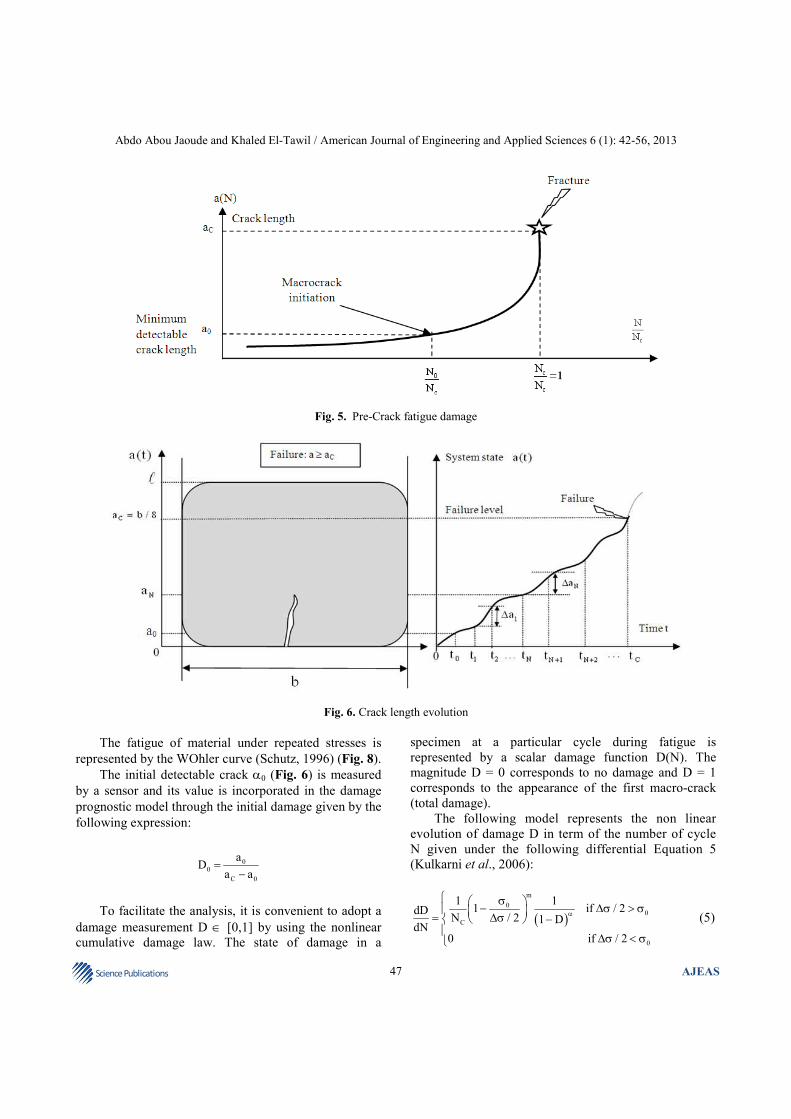
1.7. Damage Evolution Law

The fatigue of materials under cyclic loading and the

micro-cracks (starting from α0) that become detectable

and unstable (Fig. 5), will make the macro-cracks grow

to a critical length (a = aC) creating thus fractures and

hence leading to failure (Fig. 6).

The Paris law (Bartelmus and Zimroz, 2009;

Ahmad-Shariff, 2007) given by (Equation 4), where:

da

dN = The increase of the crack per

cycle

K(a) Y(a) a∆ = ∆σ π = The stress intensity factor

Y(a) = The function of the

component’s crack geometry.

∆σ = The range of the applied stress

in a cycle (σmax-σmin)

C and m = Constants of materials;

(0<C<<1); (2 ≤ m ≤ 4)

1.8. Nonlinear Cumulative Damage Modeling

1.8.1. Sensory Data Needed for Prognostic Study

To study the prognosis of a degraded component,

our idea is to predict and estimate the end of life of the

component by tracking and modeling the degradation

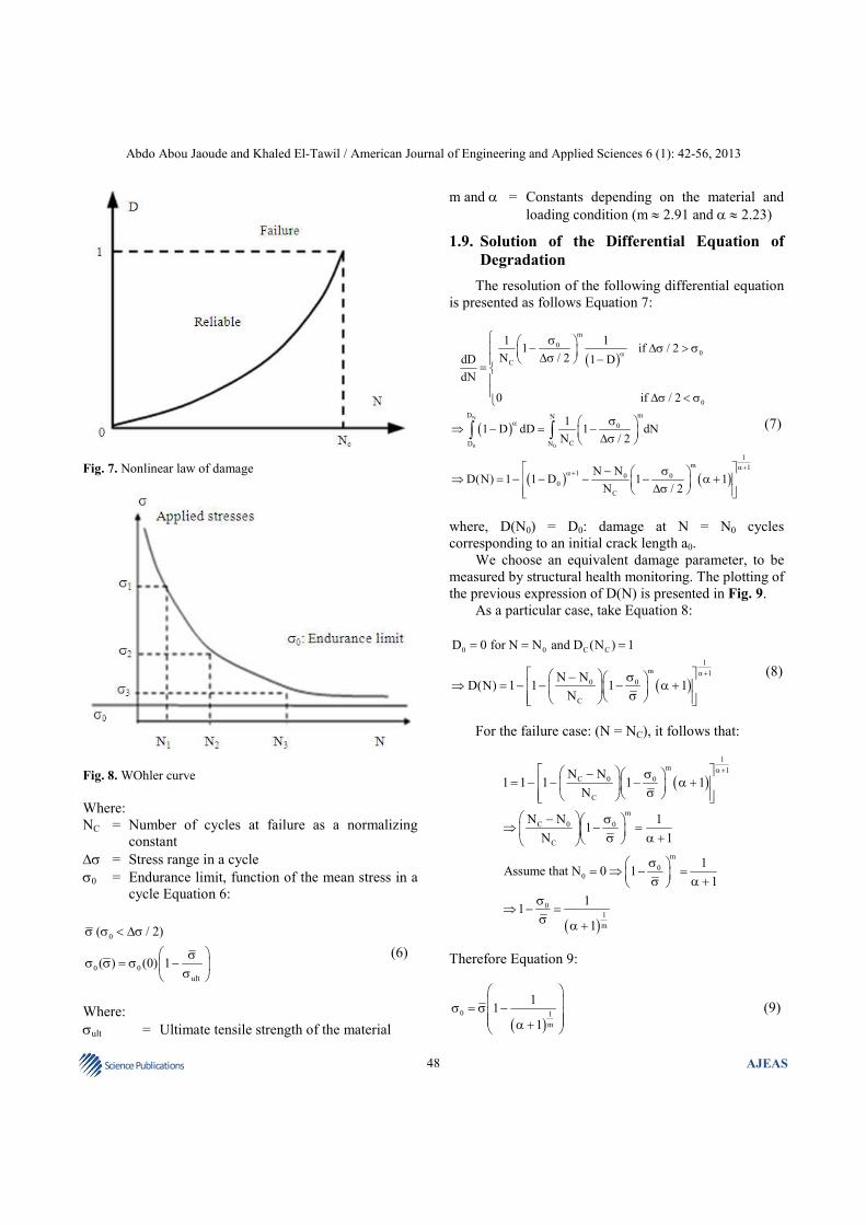
function. Our damage model, whose evolution up to the

point of macro-crack initiation, is represented in Fig. 7.



AJEAS

Fig. 5. Pre-Crack fatigue damage

Fig. 6. Crack length evolution

The fatigue of material under repeated stresses is

represented by the WOhler curve (Schutz, 1996) (Fig. 8).

The initial detectable crack α0 (Fig. 6) is measured

by a sensor and its value is incorporated in the damage

prognostic model through the initial damage given by the

following expression:

00

C 0

aD

a a=

−

To facilitate the analysis, it is convenient to adopt a

damage measurement D ∈ [0,1] by using the nonlinear

cumulative damage law. The state of damage in a

specimen at a particular cycle during fatigue is

represented by a scalar damage function D(N). The

magnitude D = 0 corresponds to no damage and D = 1

corresponds to the appearance of the first macro-crack

(total damage).

The following model represents the non linear

evolution of damage D in term of the number of cycle

N given under the following differential Equation 5

(Kulkarni et al., 2006):

( )

m

00

C

0

1 11 if / 2dD

N / 2 1 DdN

0 if / 2

α

σ − ∆σ > σ ∆σ= −

∆σ < σ

(5)



AJEAS

Fig. 7. Nonlinear law of damage

Fig. 8. WOhler curve

Where:

NC = Number of cycles at failure as a normalizing

constant

∆σ = Stress range in a cycle

σ0 = Endurance limit, function of the mean stress in a

cycle Equation 6:

0

0 0

ult

( / 2)

( ) (0) 1

σ σ < ∆σ

σσ σ = σ −

σ

(6)

Where:

σult = Ultimate tensile strength of the material

m and α = Constants depending on the material and

loading condition (m ≈ 2.91 and α ≈ 2.23)

1.9. Solution of the Differential Equation of

Degradation

The resolution of the following differential equation

is presented as follows Equation 7:

( )

( )

( ) ( )

N

0 0

m

00

C

0

mD N

0

CD N

1m 1

1 0 00

C

1 11 if / 2

N / 2dD 1 D

dN

0 if / 2

11 D dD 1 dN

N / 2

N ND(N) 1 1 D 1 1

N / 2

α

α

α+α+

σ − ∆σ > σ ∆σ −= ∆σ < σ

σ ⇒ − = − ∆σ

− σ ⇒ = − − − − α + ∆σ

∫ ∫ (7)

where, D(N0) = D0: damage at N = N0 cycles

corresponding to an initial crack length a0.

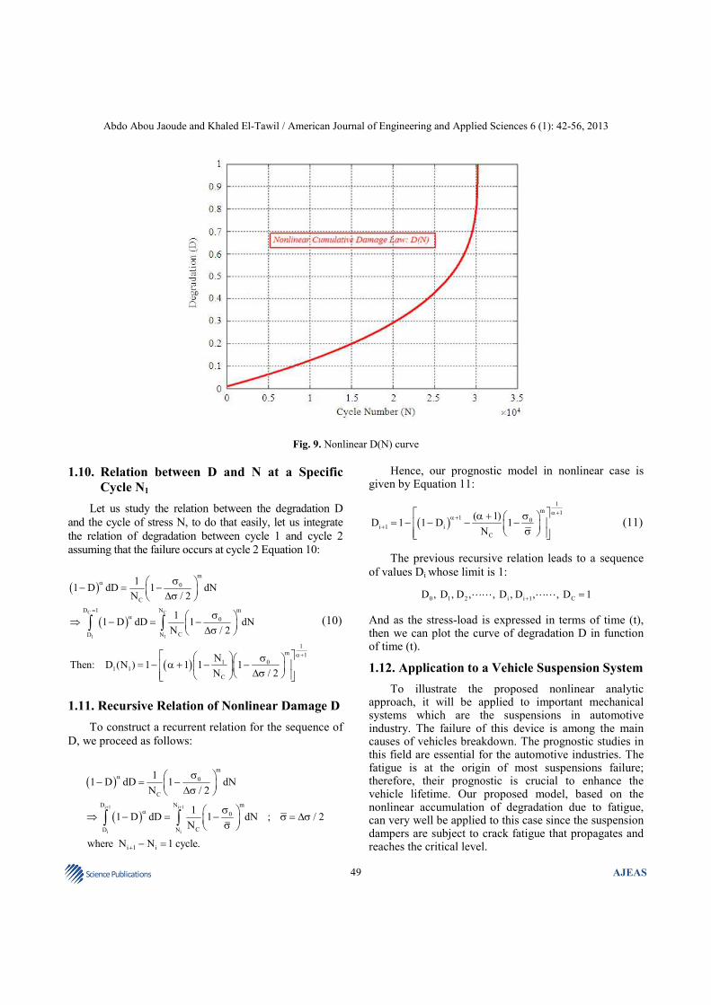
We choose an equivalent damage parameter, to be

measured by structural health monitoring. The plotting of

the previous expression of D(N) is presented in Fig. 9.

As a particular case, take Equation 8:

( )

0 0 C C

1m 1

0 0

C

D 0 for N N and D (N ) 1

N ND(N) 1 1 1 1

N

α+

= = =

− σ ⇒ = − − − α + σ

(8)

For the failure case: (N = NC), it follows that:

( )

( )

1m 1

C 0 0

C

m

C 0 0

C

m

00

0

1

m

N N1 1 1 1 1

N

N N 11

N 1

1Assume that N 0 1

1

11

1

α+ − σ = − − − α + σ

− σ ⇒ − = σ α +

σ = ⇒ − = σ α + σ

⇒ − =σ α +

Therefore Equation 9:

( )0 1

m

11

1

σ = σ − α +

(9)



AJEAS

Fig. 9. Nonlinear D(N) curve

1.10. Relation between D and N at a Specific

Cycle N1

Let us study the relation between the degradation D

and the cycle of stress N, to do that easily, let us integrate

the relation of degradation between cycle 1 and cycle 2

assuming that the failure occurs at cycle 2 Equation 10:

( )

( )

( )

C C

1 1

m

0

C

mD 1 N

0

CD N

1m 1

1 01 1

C

11 D dD 1 dN

N / 2

11 D dD 1 dN

N / 2

NThen: D (N ) 1 1 1 1

N / 2

α

=α

α+

σ − = − ∆σ

σ ⇒ − = − ∆σ

σ = − α + − − ∆σ

∫ ∫ (10)

1.11. Recursive Relation of Nonlinear Damage D

To construct a recurrent relation for the sequence of

D, we proceed as follows:

( )

( )i 1 i 1

i i

m

0

C

mD N

0

CD N

ii 1

11 D dD 1 dN

N / 2

11 D dD 1 dN ; / 2

N

where N N 1 cycle.

+ +

α

α

+

σ − = − ∆σ

σ ⇒ − = − σ = ∆σ σ

− =

∫ ∫

Hence, our prognostic model in nonlinear case is given by Equation 11:

( )

1m 1

1 0i 1 i

C

( 1)D 1 1 D 1

N

α+α+

+

α + σ = − − − − σ (11)

The previous recursive relation leads to a sequence

of values Di whose limit is 1:

0 1 2 i i 1 CD , D , D , , D , D , , D 1+ =LL LL

And as the stress-load is expressed in terms of time (t), then we can plot the curve of degradation D in function of time (t).

1.12. Application to a Vehicle Suspension System

To illustrate the proposed nonlinear analytic approach, it will be applied to important mechanical systems which are the suspensions in automotive industry. The failure of this device is among the main causes of vehicles breakdown. The prognostic studies in this field are essential for the automotive industries. The fatigue is at the origin of most suspensions failure; therefore, their prognostic is crucial to enhance the vehicle lifetime. Our proposed model, based on the nonlinear accumulation of degradation due to fatigue, can very well be applied to this case since the suspension dampers are subject to crack fatigue that propagates and reaches the critical level.



AJEAS

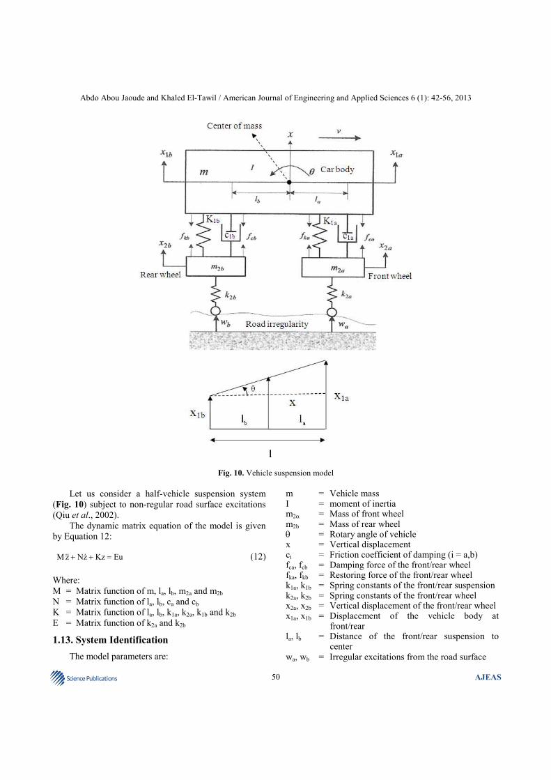
Fig. 10. Vehicle suspension model

Let us consider a half-vehicle suspension system

(Fig. 10) subject to non-regular road surface excitations

(Qiu et al., 2002).

The dynamic matrix equation of the model is given

by Equation 12:

M z Nz Kz Eu+ + =&& & (12)

Where:

M = Matrix function of m, la, lb, m2a and m2b

N = Matrix function of la, lb, ca and cb

K = Matrix function of la, lb, k1a, k2a, k1b and k2b

E = Matrix function of k2a and k2b

1.13. System Identification

The model parameters are:

m = Vehicle mass I = moment of inertia m2α = Mass of front wheel m2b = Mass of rear wheel θ = Rotary angle of vehicle x = Vertical displacement ci = Friction coefficient of damping (i = a,b) fca, fcb = Damping force of the front/rear wheel fka, fkb = Restoring force of the front/rear wheel k1a, k1b = Spring constants of the front/rear suspension k2a, k2b = Spring constants of the front/rear wheel x2a, x2b = Vertical displacement of the front/rear wheel x1a, x1b = Displacement of the vehicle body at

front/rear la, lb = Distance of the front/rear suspension to

center wa, wb = Irregular excitations from the road surface



AJEAS

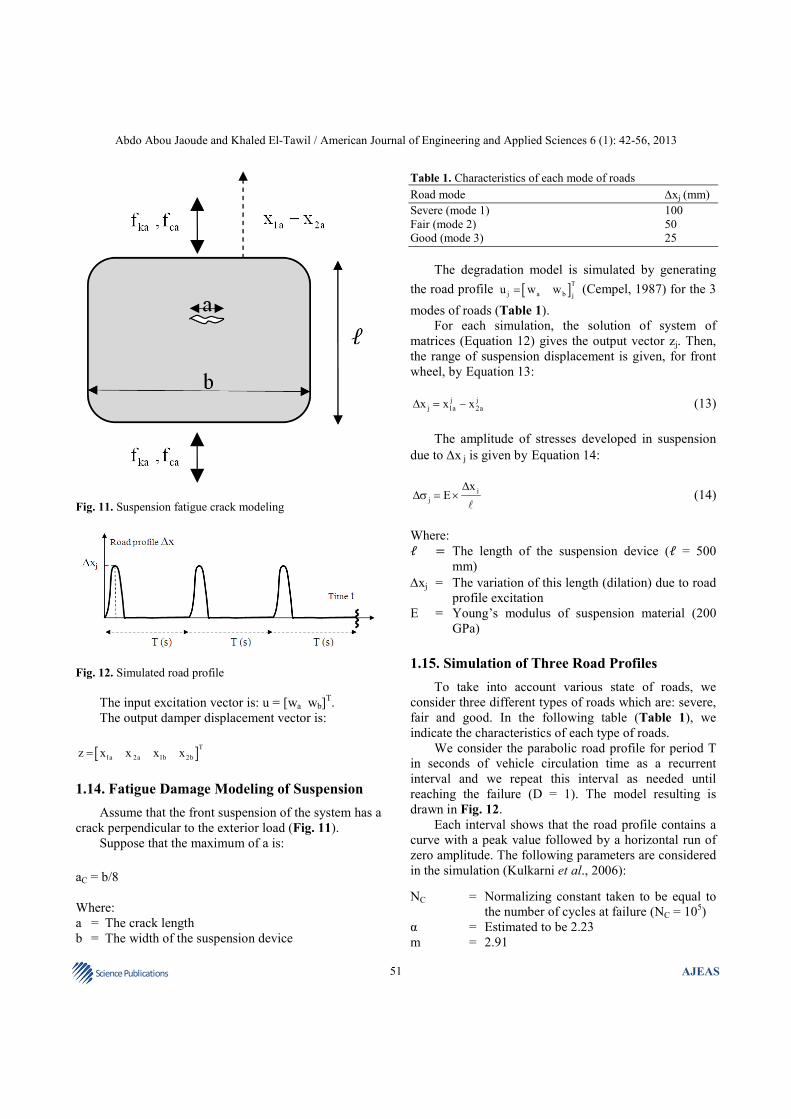
Fig. 11. Suspension fatigue crack modeling

Fig. 12. Simulated road profile

The input excitation vector is: u = [wa wb]T.

The output damper displacement vector is:

[ ]T1a 2a 1b 2bz x x x x=

1.14. Fatigue Damage Modeling of Suspension

Assume that the front suspension of the system has a

crack perpendicular to the exterior load (Fig. 11).

Suppose that the maximum of a is:

aC = b/8

Where:

a = The crack length

b = The width of the suspension device

Table 1. Characteristics of each mode of roads Road mode ∆xj (mm)

Severe (mode 1) 100

Fair (mode 2) 50

Good (mode 3) 25

The degradation model is simulated by generating

the road profile [ ]Tj a b ju w w= (Cempel, 1987) for the 3

modes of roads (Table 1).

For each simulation, the solution of system of

matrices (Equation 12) gives the output vector zj. Then,

the range of suspension displacement is given, for front

wheel, by Equation 13:

j j

j 1a 2ax x x∆ = − (13)

The amplitude of stresses developed in suspension

due to ∆x j is given by Equation 14:

j

j

xE

∆∆σ = ×

l (14)

Where:

ℓ = The length of the suspension device (ℓ = 500

mm)

∆xj = The variation of this length (dilation) due to road

profile excitation

E = Young’s modulus of suspension material (200

GPa)

1.15. Simulation of Three Road Profiles

To take into account various state of roads, we

consider three different types of roads which are: severe,

fair and good. In the following table (Table 1), we

indicate the characteristics of each type of roads.

We consider the parabolic road profile for period T

in seconds of vehicle circulation time as a recurrent

interval and we repeat this interval as needed until

reaching the failure (D = 1). The model resulting is

drawn in Fig. 12.

Each interval shows that the road profile contains a

curve with a peak value followed by a horizontal run of

zero amplitude. The following parameters are considered

in the simulation (Kulkarni et al., 2006): NC = Normalizing constant taken to be equal to

the number of cycles at failure (NC = 105)

α = Estimated to be 2.23

m = 2.91



AJEAS

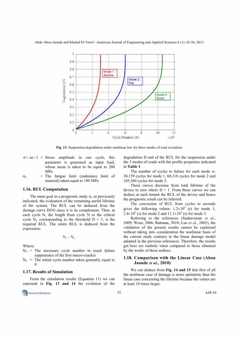
Fig. 13. Suspension degradation under nonlinear law for three modes of road excitation

/ 2σ = ∆σ = Stress amplitude in one cycle, this

parameter is generated as input load,

whose mean is taken to be equal to 280

MPa

σ0 = The fatigue limit (endurance limit of

material) taken equal to 180 MPa

1.16. RUL Computation

The main goal in a prognostic study is, as previously

indicated, the evaluation of the remaining useful lifetime

of the system. The RUL can be deduced from the

damage curve D(N) since it is its complement. Then, at

each cycle N, the length from cycle N to the critical

cycle NC corresponding to the threshold D = 1, is the

required RUL. The entire RUL is deduced from the

expression:

C 0N N−

Where:

NC = The necessary cycle number to reach failure

(appearance of the first macro-cracks)

N0 = The initial cycle number taken generally equal to

0

1.17. Results of Simulation

From the simulation results (Equation 11) we can

represent in Fig. 13 and 14 the evolution of the

degradation D and of the RUL for the suspension under

the 3 modes of roads with the profile properties indicated

in Table 1.

The number of cycles to failure for each mode is:

30,159 cycles for mode 1, 60,318 cycles for mode 2 and

105,560 cycles for mode 3.

These curves decrease from total lifetime of the

device to zero where D = 1. From these curves we can

deduce at each instant the RUL of the device and hence

the prognostic result can be inferred.

The conversion of RUL from cycles to seconds

gives the following values: 1.2×105 (s) for mode 1,

2.4×105 (s) for mode 2 and 11.1×10

5 (s) for mode 3.

Referring to the references (Sankavaram et al.,

2009; Wren, 2006; Rahman, 2010; Luo et al., 2003), the

validation of the present results cannot be explained

without taking into consideration the nonlinear basis of

the current study contrary to the linear damage model

adopted in the previous references. Therefore, the results

got here are realistic when compared to those obtained

by the works of these authors.

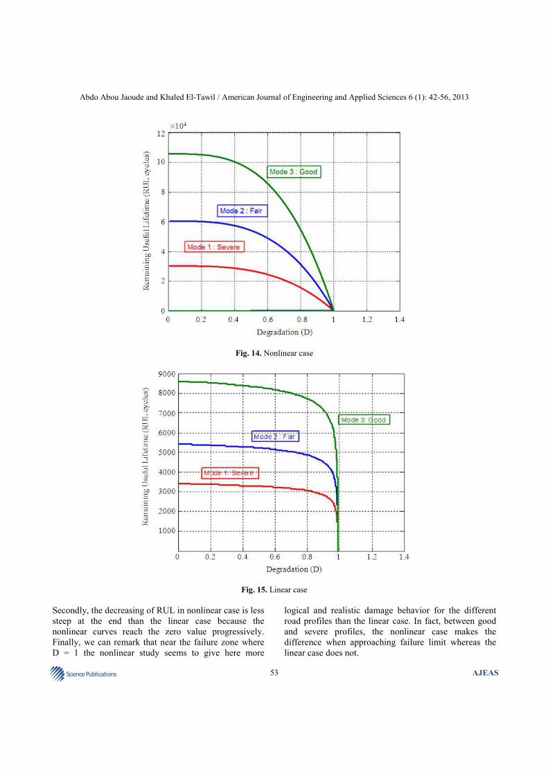
1.18. Comparison with the Linear Case (Abou

Jaoude et al., 2010)

We can deduce from Fig. 14 and 15 that first of all

the nonlinear case of damage is more optimistic than the

linear case concerning the lifetime because the values are

at least 10 times larger.



AJEAS

Fig. 14. Nonlinear case

Fig. 15. Linear case

Secondly, the decreasing of RUL in nonlinear case is less

steep at the end than the linear case because the

nonlinear curves reach the zero value progressively.

Finally, we can remark that near the failure zone where

D = 1 the nonlinear study seems to give here more

logical and realistic damage behavior for the different

road profiles than the linear case. In fact, between good

and severe profiles, the nonlinear case makes the

difference when approaching failure limit whereas the

linear case does not.



AJEAS

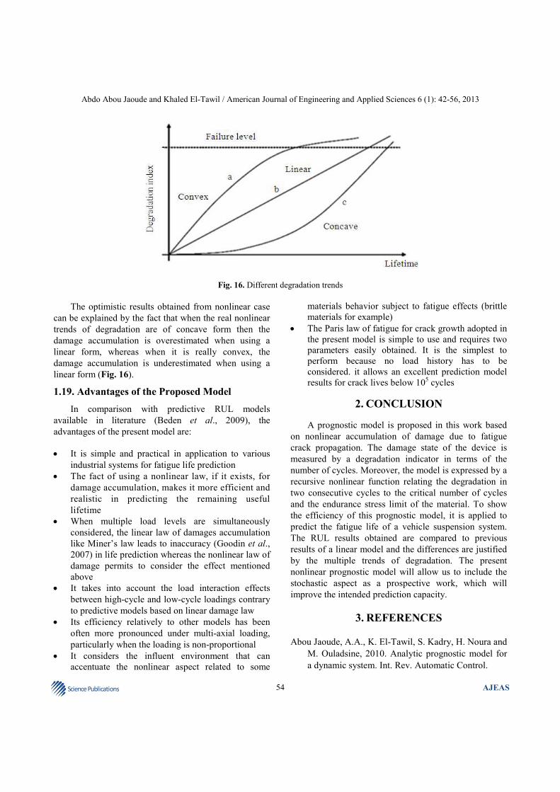
Fig. 16. Different degradation trends

The optimistic results obtained from nonlinear case

can be explained by the fact that when the real nonlinear

trends of degradation are of concave form then the

damage accumulation is overestimated when using a

linear form, whereas when it is really convex, the

damage accumulation is underestimated when using a

linear form (Fig. 16).

1.19. Advantages of the Proposed Model

In comparison with predictive RUL models

available in literature (Beden et al., 2009), the

advantages of the present model are:

• It is simple and practical in application to various

industrial systems for fatigue life prediction

• The fact of using a nonlinear law, if it exists, for

damage accumulation, makes it more efficient and

realistic in predicting the remaining useful

lifetime

• When multiple load levels are simultaneously

considered, the linear law of damages accumulation

like Miner’s law leads to inaccuracy (Goodin et al.,

2007) in life prediction whereas the nonlinear law of

damage permits to consider the effect mentioned

above

• It takes into account the load interaction effects

between high-cycle and low-cycle loadings contrary

to predictive models based on linear damage law

• Its efficiency relatively to other models has been

often more pronounced under multi-axial loading,

particularly when the loading is non-proportional

• It considers the influent environment that can

accentuate the nonlinear aspect related to some

materials behavior subject to fatigue effects (brittle

materials for example)

• The Paris law of fatigue for crack growth adopted in

the present model is simple to use and requires two

parameters easily obtained. It is the simplest to

perform because no load history has to be

considered. it allows an excellent prediction model

results for crack lives below 105 cycles

2. CONCLUSION

A prognostic model is proposed in this work based

on nonlinear accumulation of damage due to fatigue

crack propagation. The damage state of the device is

measured by a degradation indicator in terms of the

number of cycles. Moreover, the model is expressed by a

recursive nonlinear function relating the degradation in

two consecutive cycles to the critical number of cycles

and the endurance stress limit of the material. To show

the efficiency of this prognostic model, it is applied to

predict the fatigue life of a vehicle suspension system.

The RUL results obtained are compared to previous

results of a linear model and the differences are justified

by the multiple trends of degradation. The present

nonlinear prognostic model will allow us to include the

stochastic aspect as a prospective work, which will

improve the intended prediction capacity.

3. REFERENCES

Abou Jaoude, A.A., K. El-Tawil, S. Kadry, H. Noura and

M. Ouladsine, 2010. Analytic prognostic model for

a dynamic system. Int. Rev. Automatic Control.



AJEAS

Ahmad-Shariff, A., 2007. Simulation of paris-erdogan

crack propagation model: The effect of deterministic

harmonic varying stress range on the behaviour of

damage and lifetime of structure. Proceedings of the

9th Islamic Countries Conference on Statistical

Sciences, (ICCSS’ 07), pp: 12-14.

Bartelmus, W. and R. Zimroz, 2009. Vibration condition

monitoring of planetary gearbox under varying

external load. Mech. Syst. Signal Process., 23: 246-

257. DOI: 10.1016/j.ymssp.2008.03.016

Beden, S.M., S. Abdullah and A.K. Ariffin, 2009.

Review of fatigue crack propagation models for

metallic components. Eur. J. Sci. Res., 28: 364-397.

Byington, C.S., M.J. Roemer and T. Galie, 2002.

Prognostic enhancements to diagnostic systems for

improved condition-based maintenance. Proceedings

of the IEEE Aerospace Conference, (AC’ 02), IEEE

Xplore Press, pp: 6-2815-6-2824. DOI:

10.1109/AERO.2002.1036120

Cempel, C., 1987. Simple condition forecasting

techniques in vibroacoustical diagnostics. Mech.

Syst. Signal Process., 1: 75-82. DOI: 10.1016/0888-

3270(87)90084-7

Goodin, E., A. Kallmeyer and P. Kurath, 2007.

Evaluation of nonlinear cumulative damage models

for assessing HCF/LCF interactions in multiaxial

loadings. Research Report, University of Dayton

Research Institute.

Inman, D.J., C.R. Farrar, V.L. Junior and V.S. Junior,

2005. Damage Prognosis: For Aerospace, Civil and

Mechanical Systems. 1st Edn., John Wiley and

Sons, Chichester, England, ISBN-10: 0470869070,

pp: 470.

Kulkarni, S.S., L.S.B. Moran, S. Krishnaswamy and J.D.

Achenbach, 2006. A probabilistic method to predict

fatigue crack initiation. Int. J. Fracture, 137: 9-17.

DOI: 10.1007/s10704-005-3074-0

Lee, L., 2004. Smart products and service systems for e-

business transformation. Proceedings of the 3rd

Conference Francophone the Modelisation and

Simulation Conception, Analyse and Gestion this

Systemes Industriels, Apr. 25-27, Troyes, France.

Lewis, S.A. and T.G. Edwards, 1997. Smart sensors and

system health management tools for avionics and

mechanical systems. Proceedings of the 16th Digital

Avionics Systems Conference, Oct. 26-30, IEEE

Xplore Press, Irvine, CA. DOI: 10.1109/DASC.1997.637283

Luo, J., M. Namburu, K. Pattipati, L. Qiao and M.

Kawamoto et al., 2003. Model-based prognostic

techniques [maintenance applications]. Proceedings

of IEEE Systems Readiness Technology

Conference, Sept. 22-25, IEEE Xplore Press, pp:

330-340. DOI: 10.1109/AUTEST.2003.1243596

Manson, S.S. and G.R. Halford, 1981. Practical

implementation of the double linear damage rule and

damage curve approach for treating cumulative

fatigue damage. Int. J. Fatigue, 17: 169-192. DOI: 10.1007/BF00053519

Manson, S.S. and G.R. Halford, 1986. Reexamination of

Cumulative Fatigue Damage Analysis, an

engineering Perspective. 1st Edn., National

Aeronautics and Space Administration, Washington,

D.C.

Manson, S.S., J.C. Freche and C.R. Ensign, 1967.

Application of a Double Linear Damage rule to

Cumulative Fatigue. 1st Edn., National Aeronautics

and Space Administration, Washington, D.C., pp:

38.

Miner, M.A., 1945. Cumulative damage in fatigue. J.

Applied Mech., 12: A159-A164.

Paris, P.C., 1961. A rational analytic theory of fatigue.

Trend Eng., 13: 9-14.

Paris, P.C., 1963. A critical analysis of crack propagation

laws. Trans. ASME D, 85: 528-534.

Peysson, F., 2009. Contribution au pronostic des

systemes complexes, these de doctorat. Universite

d’Aix-Marseille, France.

Qiu, J., C. Zhang, B.B. Seth and S.Y. Liang, 2002.

Damage mechanics approach for bearing lifetime

prognostics. Mech. Syst. Signal Process., 16: 817-

829. DOI: 10.1006/mssp.2002.1483

Rahman, M.M., 2010. Prediction of fatigue life on lower

suspension arm subjected to variable amplitude

loading. Proceedings of the National Conference in

Mechanical Engineering Research and Postgraduate

Studies, Dec. 3-4, UMP Pekan, Pahang, pp: 100-116.

Sankavaram, C., B. Pattipati, A. Kodali, K. Pattipati and

M. Azam et al., 2009. Model-based and data-driven

prognosis of automotive and electronic systems.

Proceedings of the IEEE International Conference

on Automation Science and Engineering, Aug. 22-

25, IEEE Xplore Press, Bangalore, pp: 96-101. DOI: 10.1109/COASE.2009.5234108

Schutz, W., 1996. A history of fatigue. Eng. Fracture

Mech., 54: 263-300. DOI: 10.1016/0013-

7944(95)00178-6



AJEAS

Shigley, J. and C. Mischke, 1989. Mechanical

Engineering Design. 5th Edn., McGraw-Hill, Inc.,

pp: 310.

Vachtsevanos, G., F.L. Lewis, M. Roemer, A. Hess and

B. Wu, 2006. Intelligent Fault Diagnosis and

Prognosis for Engineering Systems. 1st Edn., John

Wiley and Sons, Hoboken, N.J., ISBN-10:

047172999X, pp: 456.

Wren, J., 2006. Fatigue and durability testing. Prosig

Noise and Vibration Measurement Blog.

Documents

Analytic and Nonlinear Prognostic for Vehicle Suspension Systems · cumulative damage theories. Ideally, the summation of life ratios would equal one at failure. However, past experiments