ANALYTIC FUNCTIONS ON TIME SCALES

A Thesis Submitted tothe Graduate School of Engineering and Sciences of

Izmir Institute of Technologyin Partial Fulfillment of the Requirements for the Degree of

MASTER OF SCIENCE

in Mathematics

bySinan KAPCAK

May 2007IZMIR

We approve the thesis of Sinan KAPCAK

Date of Signature

. . . . . . . . . . . . . . . . . . . . . . . . . . . . . . . . . . . . . 18 May 2007Assoc. Prof. Dr. Unal UFUKTEPESupervisorDepartment of MathematicsIzmir Institute of Technology

. . . . . . . . . . . . . . . . . . . . . . . . . . . . . . . . . . . . . 18 May 2007Prof. Dr. Oguz YILMAZDepartment of MathematicsIzmir Institute of Technology

. . . . . . . . . . . . . . . . . . . . . . . . . . . . . . . . . . . . . 18 May 2007Assist. Prof. Dr. Serap TOPALDepartment of MathematicsEge University

. . . . . . . . . . . . . . . . . . . . . . . . . . . . . . . . . . . . . 18 May 2007Prof. Dr. Ismail Hakkı DURUHead of DepartmentDepartment of MathematicsIzmir Institute of Technology

. . . . . . . . . . . . . . . . . . . . . . . . . . . . . . . . . .Prof. Dr. M. Barıs OZERDEM

Head of the Graduate School

ACKNOWLEDGEMENTS

I would like to express my deepest gratitude to my adviser Assoc. Prof. Dr. Unal

UFUKTEPE for his encouragement and endless support, for all that I have learnt from

him, for all the opportunities he has given to me to travel and collaborate with other

people, and most thanks for providing me his deep friendship.

I would like to thank Prof. Dr. Oguz YILMAZ and Assist. Prof. Dr. Serap

TOPAL for being in my thesis committee, it was a great honor.

My special thanks go to my dear friend Hamiyet ONBASI for her help and en-

couraging me during my thesis. I would also like to thank Aslı DENIZ for her support

and friendship.

Finally, I am deeply indepted to my family for always being with me and encour-

aging me in my life in many ways.

ABSTRACT

ANALYTIC FUNCTIONS ON TIME SCALES

The concept of analyticity for complex functions on time scale complex plane

was introduced by Bohner and Guseinov in 2005. They developed completely delta

differentiability, delta analytic functions on products of two time scales, and Cauchy-

Riemann equations for delta case.

In this thesis, beside the paper of Bohner and Guseinov, we worked on continuous,

discrete and semi-discrete analytic functions and developed completely nabla differen-

tiability, nabla analytic functions on products of two time scales, and Cauchy-Riemann

equations for nabla case.

iv

OZET

ZAMAN SKALALARINDA ANALITIK FONKSIYONLAR

Zaman skalası kompleks duzleminde kompleks fonksiyonların analitikligi

kavramı Bohner ve Guseinov tarafından 2005 yılında ortaya konulmustur. Tam delta

diferensiyellenebilme, iki zaman skalası carpımı uzerinde delta analitik fonksiyonlar ve

Cauchy-Riemann denklemlerinin delta versiyonu onlar tarafından gelistirilmistir.

Bu tezde, Bohner ve Guseinov’un makalesi yanında, surekli, kesikli ve yarı kesikli

analitik fonksiyonlar uzerine calıstık ve tam nabla diferensiyellenebilme, iki zaman

skalası carpımı uzerinde nabla analitik fonksiyonlar ve Cauchy-Riemann denklemlerinin

nabla versiyonunu gelistirdik.

v

TABLE OF CONTENTS

CHAPTER 1 . INTRODUCTION . . . . . . . . . . . . . . . . . . . . . . . . . 1

CHAPTER 2 . PRELIMINARIES . . . . . . . . . . . . . . . . . . . . . . . . . 2

2.1. Continuous Analytic Functions . . . . . . . . . . . . . . . . . 2

2.1.1. Cauchy-Riemann Equations . . . . . . . . . . . . . . . . 3

2.2. Discrete and Semi-Discrete Analytic Functions . . . . . . . . 4

2.2.1. Discrete Analytic Functions . . . . . . . . . . . . . . . . 4

2.2.2. Semi-Discrete Analytic Functions . . . . . . . . . . . . . 5

2.3. Basic Calculus on Time Scales . . . . . . . . . . . . . . . . . 7

2.3.1. Differentiation and Integration on Time Scales . . . . . . 8

CHAPTER 3 . ANALYTIC FUNCTIONS ON PRODUCTS OF TWO TIME

SCALES . . . . . . . . . . . . . . . . . . . . . . . . . . . . . . . . . . . . . 13

3.1. Functions of Two Real Time Scale Variables . . . . . . . . . . 13

3.1.1. Completely Delta Differentiable Functions . . . . . . . . 13

3.1.2. Completely Nabla Differentiable Functions . . . . . . . . 15

3.2. Cauchy-Riemann Equations on Time Scale Complex Plane . . 19

3.2.1. Delta Analytic Functions . . . . . . . . . . . . . . . . . . 20

3.2.2. Nabla Analytic Functions . . . . . . . . . . . . . . . . . 25

CHAPTER 4 . CONCLUSION . . . . . . . . . . . . . . . . . . . . . . . . . . 30

REFERENCES . . . . . . . . . . . . . . . . . . . . . . . . . . . . . . . . . . . 31

vi

CHAPTER 1

INTRODUCTION

Time Scale Calculus was developed earlier in (Hilger 1997, Guseinov 2003,

Bohner and Peterson 2001). Gusein Sh. Guseinov and Martin Bohner gave the differ-

ential calculus, integral calculus and developed line integration along time scale curves

(Bohner and Guseinov 2004 and Guseinov 2003). They also developed the concept of

analytic functions on Time Scales in (Bohner and Guseinov 2005).

This thesis is organized as follows. In chapter two, we gave the review of the

analytic functions on complex plane, Cauchy-Riemann equations and their properties. In

the same chapter we gave discrete and semi-discrete analogs of analytic functions. We

also presented the basic time scale calculus concepts and their classical results in chapter

two.

In chapter three, we worked on the paper of Gusein Sh. Guseinov and Martin

Bohner (Bohner and Guseinov 2005) on analytic functions on products of two time

scales, functions of two time scales variables, ∆ and ∇ differentiable functions on

products of two time scales, Cauchy-Riemann equations on products of two time scales

and ∆-analytic functions.

In addition, we have developed completely ∇-differentiability, ∇-analytic func-

tions on products of two time scales, Cauchy-Riemann equations for nabla case.

1

CHAPTER 2

PRELIMINARIES

2.1. Continuous Analytic Functions

Suppose that D ⊆ C is a domain. A function f : D → C is said to be differen-

tiable at z0 ∈ D if the limit

limz→z0

f(z)− f(z0)

z − z0

exists. In this case, we write

f ′(z0) = limz→z0

f(z)− f(z0)

z − z0

, (2.1)

and call f ′(z0) the derivative of f at z0.

If z 6= z0, then

f(z) =

(f(z)− f(z0)

z − z0

)(z − z0) + f(z0).

It follows from (2.1) that if f ′(z0) exists, then f(z) → f(z0) as z → z0, so that f is

continuous at z0. In other words, differentiability at z0 implies continuity at z0.

If the functions f : D → C and g : D → C are both differentiable at z0 ∈ D, then

both f + g and fg are differentiable at z0, and

(f + g)′(z0) = f ′(z0) + g′(z0) and (fg)′(z0) = f(z0)g′(z0) + f ′(z0)g(z0).

If the extra condition g′(z0) 6= 0 holds, then f/g is differentiable at z0, and(f

g

)′

(z0) =g(z0)f

′(z0)− f(z0)g′(z0)

g2(z0).

Example 1. Consider the function f(z) = z, where for every z ∈ C, z denotes the

complex conjugate of z. Suppose that z0 ∈ C. Then

f(z)− f(z0)

z − z0

=z − z0

z − z0

=z − z0

z − z0

. (2.2)

If z − z0 = h is real and non-zero, then (2.2) takes the value 1. On the other hand, if

z−z0 = ik is purely imaginary, then (2.2) takes the value−1. It follows that this function

is not differentiable anywhere in C, although its real and imaginary parts are rather well

behaved.

2

2.1.1. Cauchy-Riemann Equations

If we use the notation

f ′(z) = limh→0

f(z + h)− f(z)

h,

then in Example 1, we have examined the behaviour of the ratio

f(z + h)− f(z)

h

first as h → 0 through real values and then through imaginary values. Indeed, for the

derivative to exist, it is essential that these two limiting processes produce the same limit

f ′(z). Suppose that f(z) = u(x, y) + iv(x, y), where, z = x + iy, and u and v are real

valued functions. If h is real, then the two limiting processes above correspond to

limh→0

f(z + h)− f(z)

h= lim

h→0

u(x + h, y)− u(x, y)

h+ i lim

h→0

v(x + h, y)− v(x, y)

h

=∂u

∂x+ i

∂v

∂x

and

limh→0

f(z + ih)− f(z)

ih= lim

h→0

u(x, y + h)− u(x, y)

ih+ i lim

h→0

v(x, y + h)− v(x, y)

ih

=∂v

∂y− i

∂u

∂y

respectively. Equating real and imaginary parts, we obtain

∂u

∂x=

∂v

∂yand

∂u

∂y= −∂v

∂x. (2.3)

Definition 2. The partial differential equations (2.3) are called the Cauchy-Riemann

equations.

Theorem 3. Suppose that f(z) = u(x, y) + iv(x, y), where z = x + iy, and u and v are

real valued functions. Suppose further that f ′(z) exists. Then the four partial derivatives

in (2.3) exist, and the Cauchy-Riemann equations (2.3) hold. Furthermore, we have

f ′(z) =∂u

∂x+ i

∂v

∂xand f ′(z) =

∂v

∂y− i

∂u

∂y. (2.4)

Theorem 4. Suppose that f(z) = u(x, y) + iv(x, y), where z = x + iy, and u and

v are real valued functions. Suppose further that the four partial derivatives in (2.3) are

continuous and satisfy the Cauchy-Riemann equations (2.3) at z0. Then f is differentiable

at z0, and the derivative f ′(z0) is given by the equations (2.4) evaluated at z0.

3

Definition 5. A function f is said to be analytic at a point z0 ∈ C if it is differentiable at

every z in some ε-neighbourhood of the point z0. The function f is said to be analytic in

a region if it is analytic at every point in the region. The function f is said to be entire if

it is analytic in C.

2.2. Discrete and Semi-Discrete Analytic Functions

The theory of discrete and semi-discrete functions is obtained by deriving

satisfactory analogues of classical results in the theory of analytic functions as well

as finding results which have no direct analog in the classic theory. The study of

analytic functions on Z2 has a history of more than sixty years. The pioneer in that

field is Rufus Isaacs (Isaacs 1941), who introduced two difference equations, both of

which are discrete counterparts of the Cauchy-Riemann equation in one complex variable.

The discrete analogues of analytic functions have been called by several names.

Duffin (Duffin 1956) calls them discrete analytic functions, Ferrand (Ferrand 1944)

calls them preholomorphic functions, and Isaacs (Isaacs 1941) calls them monodiffric

functions. In this thesis we will use the definitions given by Isaacs.

2.2.1. Discrete Analytic Functions

Definition 6. A complex-valued function f defined on a subset A of Z + iZ is said to be

holomorphic in the sense of Isaacs or monodiffric (discrete analytic) of the first kind if the

equationf(z + 1)− f(z)

1=

f(z + i)− f(z)

i(2.5)

holds for all z ∈ A such that also z + 1 and z + i belong to A.

It should be noted that this definition is not the one used by Duffin or Ferrand in

their works on discrete analytic functions.

In (Isaacs 1941) Isaacs defined also monodiffric functions of the second kind, in

which the condition

f(z0 + 1 + i)− f(z0)

1 + i=

f(z0 + i)− f(z0 + 1)

i− 1(2.6)

4

is required instead of (2.5).

Here, we propose a new kind of monodiffric function which we call backward

monodiffric function. To avoid confusion we call the monodiffric function of first kind as

forward monodiffric function.

Definition 7. A complex-valued function f defined on a subset A of Z + iZ is said to be

backward monodiffric if the equation

f(z)− f(z − 1)

1=

f(z)− f(z − i)

i(2.7)

holds for all z ∈ A such that also z − 1 and z − i belong to A.

There are many papers which concern discrete analogues for analytic functions

by Duffin and Isaacs. In each of these, either a discrete analogue to the Cauchy-Riemann

equations or in the case of Ferrand, a discrete version of Morera’s theorem is used to

define discrete analytic functions (as (2.5) and (2.6)).

2.2.2. Semi-Discrete Analytic Functions

Semi-discrete analytic functions are single-valued functions of one continuous

and one discrete variable defined on a semi-lattice, a uniformly spaced sequence of lines

parallel to the real axis.

The appropriate semi-discrete analogues of analytic functions are defined in

(Kurowski 1963) from the classic Cauchy-Riemann equations on replacing the y-

derivative by either a nonsymmetric difference

∂f(z)

∂x= [f(z + ih)− f(z)]/ih, z = x + ikh, (2.8)

or a symmetric difference

∂f(z)

∂x= [f(z + ih/2)− f(z − ih/2)]/ih, z = x + ikh/2. (2.9)

Definition 8. Semi-discrete functions which satisfy (2.8) or (2.9) are called, respectively,

semi-discrete analytic functions of the first, second kind.

5

In this thesis we will deal with the semi-discrete analytic functions of the first kind

and because we will propose the backward version of semi-discrete analytic functions, to

avoid confusion we call the first kind, forward semi-discrete analytic functions.

Definition 9. The function defined on R + ihZ that satisfies the condition

∂f(z)

∂x= [f(z)− f(z − ih)]/ih, z = x + ikh, (2.10)

is called backward semi-discrete analytic function.

Let f(z) = u(x, y)+ iv(x, y) be semi-discrete analytic function on D ⊂ R+ ihZ,

where u and v are real valued semi-discrete functions, equating real and imaginary parts

of (2.8) and (2.9) respectively yields the semi-discrete Cauchy-Riemann equations. For

Type I∂u(x, y)

∂x=

1

h[v(x, y + h)− v(x, y)],

∂v(x, y)

∂x=

1

h[u(x, y)− u(x, y + h)],

and for Type II∂u(x, y)

∂x=

1

h[v(x, y +

h

2)− v(x, y − 1

2)],

∂v(x, y)

∂x=

1

h[u(x, y − h

2)− u(x, y +

h

2)].

Helmbold (Helmbold ) considers functions on a semi-lattice which satisfies the

following semi-discrete analogue of Laplace’s equation:

d2u(x, k)

dx2+ [u(x, k + 1)− 2u(x, k) + u(x, k − 1)] = 0. (2.11)

He calls this function semi-discrete harmonic.

Let us introduce following operators on D which are defined by Kurowski in

(Kurowski 1963).

(a) ∆1f(z) = f(z + ih)− f(z),

(b) ∆2f(z) = f(z + ih/2)− f(z − ih/2),

(c) ∆n+1j = ∆j[∆

nj f(z)], n ≥ 1,

(d) ∇jf(z) = ∂2f(z)∂x2 + ∆2

jf(z),

(e) 2Sjf(z) = ∂f(z)∂x

− ih∆jf(z),

6

(f) 2Sjf(z) = ∂f(z)∂x

+ ih∆jf(z),

(g) 2SBf(z) = ∂f(z)∂x

+ ih∆1f(z − ih).

Since

4Sj[Sj(f)] = 4Sj[Sj(f)] = ∇j(f),

if f(z) is semi-discrete analytic on D, then ∇j(f) = 0 for all z ∈ D0 and consequently

∇j(u) = ∇j(v) = 0.

Semi-discrete functions g such that ∇j(g) = 0 are called semi-discrete harmonic func-

tions of the first or second kind. The semi-discrete functions of the second kind are

the semi-discrete harmonic functions considered by Helmbold (Helmbold ), see equation

(2.11), who called such functions 1/2-harmonic.

2.3. Basic Calculus on Time Scales

By a time scale T, we mean an arbitrary nonempty closed subset of real numbers.

The set of the real numbers, the integers, the natural numbers, and the Cantor set are

examples of time scales. But the rational numbers, the irrational numbers, the complex

numbers, and the open interval between 0 and 1, are not time scales.

The calculus of time scales was introduced by Stefan Hilger in his 1988 Ph.D.

dissertation (Hilger 1997) in order to create the theory that can unify the discrete and

continuous analysis. After discovery of time scales in 1988 almost every result obtained

in the theory of differential and difference equations are carried into time scales.

In order to define ∆ derivative (∇ derivative) we need to define forward jump

operator σ, (backward jump operator ρ), graininess function µ (ν), and the region of

differentiability Tκ (Tκ) which is derived from T.

Definition 10. Let T be a time scale. The forward jump operator σ : T → T is defined

by

σ(t) = inf{s ∈ T : s > t} , ∀t ∈ T

7

and the backward jump operator ρ : T → T is defined by

ρ(t) = sup{s ∈ T : s < t} , ∀t ∈ T.

Also σ(max(T)) = max(T) and ρ(min(T)) = min(T). t is called right dense if σ(t) = t,

left dense if ρ(t) = t and right scattered if σ(t) > t, left scattered if ρ(t) < t. t is called

dense point if t is both left and right dense, and t is isolated if it is both left and right

scattered. The graininess functions µ : T → [0,∞) and ν : T → [0,∞) are defined by

µ(t) = σ(t)− t and ν(t) = t− ρ(t).

If T = R, then we have for any t ∈ R

σ(t) = inf{s ∈ R : s > t} = inf(t,∞) = t

and similarly ρ(t) = t. Hence every point t ∈ R is dense. The graininess functions µ and

ν turn out to be µ(t) = ν(t) = 0 for all t ∈ R.

If T = Z, then we have for any t ∈ Z

σ(t) = inf{s ∈ Z : s > t} = inf{t + 1, t + 2, · · · } = t + 1

and similarly ρ(t) = t− 1. Hence every point t ∈ Z is isolated. The graininess functions

µ and ν turn out to be µ(t) = ν(t) = 1 for all t ∈ Z.

We define the interval [a, b] in T by

[a, b] = {t ∈ T : a ≤ t ≤ b}.

2.3.1. Differentiation and Integration on Time Scales

Let T be a nonempty closed subset of the real numbers R. T has the topology

that it inherits from the real numbers with the standard topology. Let σ(t) and ρ(t) be the

forward and backward jump operators in T, respectively. We introduce the sets Tκ and

Tκ which are derived from the time scale T as follows. If T has a left-scattered maximum

t1, then Tκ = T − {t1}, otherwise Tκ = T. If T has right-scattered minimum t2, then

Tκ = T− {t2}, otherwise Tκ = T.

If f : T → R is a function and t ∈ Tκ, then the delta derivative of f at the point

t is defined to be the number f∆(t) (provided it exists) with the property that for each

8

ε > 0 there is neighborhood U of t such that

|f(σ(t))− f(s)− f∆(t)[σ(t)− s]| ≤ ε|σ(t)− s| for all s ∈ U.

If t ∈ Tκ, then we define the nabla derivative of f at the point t to be the number

f∇(t) (provided it exists) with the property that for each ε > 0 there is neighborhood U

of t such that

|f(ρ(t))− f(s)− f∇(t)[ρ(t)− s]| ≤ ε|ρ(t)− s| for all s ∈ U.

A function F : T → R is called a ∆-antiderivative of f : T → R provided

F∆(t) = f(t) holds for all t ∈ Tκ. Then Cauchy ∆-integral from a to t of f is defined by∫ t

a

f(s)∆s = F (t)− F (a) for all t ∈ T.

A function Φ : T → R is called a ∇-antiderivative of f : T → R provided

Φ∇(t) = f(t) holds for all t ∈ Tκ. Then Cauchy ∇-integral from a to t of f is defined by∫ t

a

f(s)∇s = Φ(t)− Φ(a) for all t ∈ T.

Note that in the case T = R, we have

f∆(t) = f∇(t) = f ′(t),

∫ b

a

f(t)∆t =

∫ b

a

f(t)∇t =

∫ b

a

f(t)dt,

and in the case T = Z, we have

f∆(t) = f(t + 1)− f(t), f∇(t) = f(t)− f(t− 1),∫ b

a

f(t)∆t =b−1∑k=a

f(k),

∫ b

a

f(t)∇t =b∑

k=a+1

f(k),

where a, b ∈ T with a ≤ b.

The following theorems give several properties of the delta and nabla derivatives;

they are found in (Bohner and Peterson 2001 and Merdivenci and Guseinov 2002).

9

Theorem 11. For f : T → R and t ∈ Tκ the following hold.

(i) If f is ∆-differentiable at t, then f is continuous at t.

(ii) If f is continuous at t and t is right-scattered, then f is ∆-differentiable at t and

f∆(t) =f(σ(t))− f(t)

σ(t)− t.

(iii) If t is right-dense, then f is ∆-differentiable at t if and only if the limit

lims→t

f(t)− f(s)

t− s

exist as a finite number. In the case f∆(t) is equal to this limit.

(iv) If f is ∆-differentiable at t, then

f(σ(t)) = f(t) + [σ(t)− t]f∆(t).

Theorem 12. Assume that f, g : T → R are ∆-differentiable at t ∈ Tκ. Then for

α, β ∈ R

(i) The linear sum αf + βg : T → R is ∆-differentiable at t with

(αf + βg)∆(t) = αf∆(t) + βg∆(t)

(ii) The product (fg) : T → R is ∆-differentiable at t with

(fg)∆(t) = f∆(t)g(t) + f(σ(t))g∆(t) = f(t)g∆(t) + f∆(t)g(σ(t)).

(iii) If g(t)g(σ(t)) 6= 0 thenf

gis ∆-differentiable at t with

(f

g

)∆

(t) =f∆(t)g(t)− f(t)g∆(t)

g(t)g(σ(t)).

Theorem 13. For f : T → R and t ∈ Tκ the following hold.

(i) If f is ∇-differentiable at t, then f is continuous at t.

(ii) If f is continuous at t and t is left-scattered, then f is ∇-differentiable at t and

f∇(t) =f(ρ(t))− f(t)

ρ(t)− t.

10

(iii) If t is left-dense, then f is ∇-differentiable at t if and only if the limit

lims→t

f(t)− f(s)

t− s

exist as a finite number. In the case f∇(t) is equal to this limit.

(iv) If f is ∇-differentiable at t, then

f(ρ(t)) = f(t) + [ρ(t)− t]f∇(t).

Theorem 14. Assume that f, g : T → R are ∇-differentiable at t ∈ Tκ. Then for

α, β ∈ R

(i) The linear sum αf + βg : T → R is ∇-differentiable at t with

(αf + βg)∇(t) = αf∇(t) + βg∇(t)

(ii) The product (fg) : T → R is ∇-differentiable at t with

(fg)∇(t) = f∇(t)g(t) + f(ρ(t))g∇(t) = f(t)g∇(t) + f∇(t)g(ρ(t)).

(iii) If g(t)g(ρ(t)) 6= 0 thenf

gis ∇-differentiable at t with

(f

g

)∇

(t) =f∇(t)g(t)− f(t)g∇(t)

g(t)g(ρ(t)).

Example 15. We consider the function f(t) = t2 on an arbitrary time scale.

Let T be an arbitrary time scale and t ∈ Tκ. The ∆-derivative of f is given by

f∆(t) = lims→t

f(σ(t))− f(s)

σ(t)− s= lim

s→t

(σ(t))2 − s2

σ(t)− s= lim

s→tσ(t) + s = σ(t) + t.

1. If T = R then σ(t) = t. Therefore f∆(t) = f ′(t) = 2t

2. If T = Z then σ(t) = t + 1. Therefore f∆(t) = ∆f(t) = 2t + 1.

3. If T = N120 = {

√n : n ∈ N0} then σ(t) =

√t2 + 1. Therefore

f∆(t) = t +√

t2 + 1.

Similarly, to find ∇-derivative, let us take t ∈ Tκ. The ∇-derivative of f is given

by

f∇(t) = lims→t

f(ρ(t))− f(s)

ρ(t)− s= lim

s→t

(ρ(t))2 − s2

ρ(t)− s= lim

s→tρ(t) + s = ρ(t) + t.

11

1. If T = R then ρ(t) = t. Therefore f∇(t) = f ′(t) = 2t

2. If T = Z then ρ(t) = t− 1. Therefore f∇(t) = ∇f(t) = 2t− 1.

3. If T = N120 = {

√n : n ∈ N0} then ρ(t) =

√t2 − 1. Therefore

f∇(t) = t−√

t2 − 1.

Theorem 16. Assume a, b, c ∈ T, then

(i)∫ b

a[f(t)g(t)]∆t =

∫ b

af(t)∆t +

∫ b

ag(t)∆t,∫ b

a[f(t)g(t)]∇t =

∫ b

af(t)∇t +

∫ b

ag(t)∇t

(ii)∫ b

akf(t)∆t = k

∫ b

af(t)∆t,

∫ b

akf(t)∇t = k

∫ b

af(t)∇t

(iii)∫ b

af(t)∆t = −

∫ a

bf(t)∆t,

∫ b

af(t)∇t = −

∫ a

bf(t)∇t

(iv)∫ b

af(t)∆t =

∫ c

af(t)∆t +

∫ b

cf(t)∆t,

∫ b

af(t)∇t =

∫ c

af(t)∇t +

∫ b

cf(t)∇t

(v)∫ b

af∆(t)g(t)∆t = f(t)g(t)|ba −

∫ b

af(σ(t))g∆(t)∆t,∫ b

af∇(t)g(t)∇t = f(t)g(t)|ba −

∫ b

af(ρ(t))g∇(t)∆t

12

CHAPTER 3

ANALYTIC FUNCTIONS ON PRODUCTS OF TWO

TIME SCALES

3.1. Functions of Two Real Time Scale Variables

Let T1 and T2 be time scales. Let us set T1 × T2 = {(x, y) : x ∈ T1, y ∈ T2}.

The set T1 × T2 is a complete metric space with the metric (distance) d defined by

d((x, y), (x′, y′)) =√

(x− x′)2 + (y − y′)2 for (x, y), (x′, y′) ∈ T1 × T2.

For a given δ > 0, the δ-neighborhood Uδ(x0, y0) of a given point (x0, y0) ∈ T1 × T2

is the set of all points (x, y) ∈ T1 × T2 such that d((x0, y0), (x, y)) < δ. Let σ1 and σ2

be the forward jump operators for T1 and T2, respectively. Further, let ρ1 and ρ2 be the

backward jump operators for T1 and T2, respectively. Let u : T1×T2 → R be a function.

The first order delta derivatives of u at a point (x0, y0) ∈ Tκ1 × Tκ

2 are defined to be

∂u(x0, y0)

∆1x= lim

x→x0,x 6=σ1(x0)

u(σ1(x0), y0)− u(x, y0)

σ1(x0)− x

and∂u(x0, y0)

∆2y= lim

y→y0,y 6=σ2(y0)

u(x0, σ2(y0))− u(x0, y)

σ2(y0)− y.

Similarly, we define nabla derivatives of u at a point (x0, y0) ∈ T1κ × T2κ as

∂u(x0, y0)

∇1x= lim

x→x0,x 6=ρ1(x0)

u(x, y0)− u(ρ1(x0), y0)

x− ρ1(x0)

and∂u(x0, y0)

∇2y= lim

y→y0,y 6=ρ2(y0)

u(x0, y)− u(x0, ρ2(y0))

y − ρ2(y0).

3.1.1. Completely Delta Differentiable Functions

Before the definition of completely delta differentiability on products of two time

scales, we first give the definition for one-variable case.

13

Definition 17. A function u : T → R is called completely delta differentiable at a point

x0 ∈ Tκ if there exists a number A such that

u(x0)− u(x) = A(x0 − x) + α(x0 − x) for all x ∈ Uδ(x0) (3.1)

and

u(σ(x0))− u(x) = A[σ(x0)− x] + β[σ(x0)− x] for all x ∈ Uδ(x0) (3.2)

where α = α(x0, x) and β = β(x0, x) are equal zero at x = x0 and

limx→x0

α(x0, x) = 0 and limx→x0

β(x0, x) = 0.

Now we can give the definition for two variable case:

Definition 18. We say that a function u : T1×T2 → R is completely delta differentiable

at a point (x0, y0) ∈ Tκ1 × Tκ

2 if there exist numbers A1 and A2 independent of (x, y) ∈

T1 × T2 (but, in general, dependent on (x0, y0)) such that

u(x0, y0)− u(x, y) = A1(x0 − x) + A2(y0 − y) + α1(x0 − x) + α2(y0 − y), (3.3)

u(σ1(x0), y0)−u(x, y) = A1[σ1(x0)−x]+A2(y0−y)+β11[σ1(x0)−x]+β12(y0−y), (3.4)

u(x0, σ2(y0))−u(x, y) = A1(x0−x)+A2[σ2(y0)−y]+β21[x0−x]+β22[σ2(y0)−y] (3.5)

for all (x, y) ∈ Uδ(x0, y0), where δ > 0 is sufficiently small, αj = αj(x0, y0; x, y)

and βjk = βjk(x0, y0; x, y) are defined on Uδ(x0, y0) such that they are equal to zero

at (x, y) = (x0, y0) and

lim(x,y)→(x0,y0)

αj(x0, y0; x, y) = lim(x,y)→(x0,y0)

βjk(x0, y0; x, y) = 0 for j, k ∈ {1, 2}

Note that in case T1 = T2 = Z, the neighborhood Uδ(x0, y0) contains the single

point (x0, y0) for δ < 1. Therefore, in the case, the condition (3.3) disappears, while the

conditions (3.4) and (3.5) hold with βjk = 0 and with

A1 = u(x0 + 1, y0)− u(x0, y0) =∂u(x0, y0)

∆1x(3.6)

and

A2 = u(x0, y0 + 1)− u(x0, y0) =∂u(x0, y0)

∆2y. (3.7)

14

Lemma 19. Let the function u : T1 × T2 → R be completely delta differentiable at the

point (x0, y0) ∈ Tκ1 × Tκ

2 , then it is continuous at that point and has at (x0, y0) the first

order partial delta derivatives equal to A1 and A2, namely

∂u(x0, y0)

∆1x= A1 and

∂u(x0, y0)

∆2y= A2.

Proof. The continuity of u follows, in fact, from any one of (3.3), (3.4) and (3.5). Indeed

(3.3) obviously yields the continuity of u at (x0, y0). Let now (3.4) holds. In the case

σ1(x0) = x0, (3.4) immediately gives the continuity of u at (x0, y0). If σ1(x0) > x0,

except of u(x, y), each term in (3.4) has a limit as (x, y) → (x0, y0). Therefore u(x, y)

also has a limit as (x, y) → (x0, y0), and we have

u(σ1(x0), y0)− lim(x,y)→(x0,y0)

u(x, y) = A1[σ1(x0)− x0].

Further, letting (x, y) = (x0, y0) in (3.4), we get

u(σ1(x0), y0)− u(x0, y0) = A1[σ1(x0)− x0].

Comparing the last two relations gives

lim(x,y)→(x0,y0)

u(x, y) = u(x0, y0)

which shows the continuity of u at (x0, y0). Next, setting y = y0 in (3.4) and dividing

both sides by σ1(x0)−x and passing to limit as x → x0 we get ∂u(x0,y0)∆1x

= A1. By similar

approach ∂u(x0,y0)∆2y

= A2 can be obtained.

3.1.2. Completely Nabla Differentiable Functions

Before the definition of completely nabla differentiability on products of two time

scales, we first give the definition for one-variable case.

Definition 20. A function u : T → R is called completely nabla differentiable at a point

x0 ∈ Tκ if there exists a number B such that

u(x)− u(x0) = B(x− x0) + α(x− x0) for all x ∈ Uδ(x0) (3.8)

and

u(x)− u(ρ(x0)) = B[x− ρ(x0)] + β[x− ρ(x0)] for all x ∈ Uδ(x0) (3.9)

15

where α = α(x0, x) and β = β(x0, x) are equal zero at x = x0 and

limx→x0

α(x0, x) = 0 and limx→x0

β(x0, x) = 0.

Now we can give the definition for two variable case:

Definition 21. We say that a function u : T1×T2 → R is completely nabla differentiable

at a point (x0, y0) ∈ T1κ × T2κ if there exist numbers B1 and B2 independent of (x, y) ∈

T1 × T2 (but, in general, dependent on (x0, y0)) such that

u(x, y)− u(x0, y0) = B1(x− x0) + B2(y − y0) + α1(x− x0) + α2(y − y0), (3.10)

u(x, y)− u(ρ1(x0), y0) = B1[x− ρ1(x0)] + B2(y− y0) + β11[x− ρ1(x0)] + β12(y− y0),

(3.11)

u(x, y)−u(x0, ρ2(y0)) = B1(x−x0)+B2[y−ρ2(y0)]+β21[x−x0]+β22[y−ρ2(y0)] (3.12)

for all (x, y) ∈ Uδ(x0, y0), where δ > 0 is sufficiently small, αj = αj(x0, y0; x, y)

and βjk = βjk(x0, y0; x, y) are defined on Uδ(x0, y0) such that they are equal to zero

at (x, y) = (x0, y0) and

lim(x,y)→(x0,y0)

αj(x0, y0; x, y) = lim(x,y)→(x0,y0)

βjk(x0, y0; x, y) = 0 for j, k ∈ {1, 2}

With T1 = T2 = Z, similarly we have

B1 = u(x0, y0)− u(x0 − 1, y0) =∂u(x0, y0)

∇1x

and

B2 = u(x0, y0)− u(x0, y0 − 1) =∂u(x0, y0)

∇2y.

This results and (3.6) and (3.7) show that each function u : Z × Z → R is completely

delta and nabla differentiable at every point.

Lemma 22. Let the function u : T1 × T2 → R be completely nabla differentiable at the

point (x0, y0) ∈ T1κ × T2κ, then it is continuous at that point and has at (x0, y0) the first

order partial nabla derivatives equal to B1 and B2, namely

∂u(x0, y0)

∇1x= B1 and

∂u(x0, y0)

∇2y= B2.

Proof. The proof is similar with the Lemma 19.

16

Theorem 23. If the function u : T1×T2 → R is continuous and have the first order partial

nabla derivatives ∂u(x,y)∇1x

, ∂u(x,y)∇2y

in some δ-neighborhood Uδ(x0, y0) of the point (x0, y0) ∈

T1κ × T2κ and if these derivatives are continuous at (x0, y0), then u is completely ∇-

differentiable at (x0, y0).

To prove this theorem we first give the mean value theorem for one-variable case.

Theorem 24. Let a and b be two arbitrary points in T and let us set α = min{a, b}

and β = max{a, b}. Let, further, f be a continuous function on [α, β] that has a nabla

derivative at each point of (α, β]. Then there exist ξ, ξ′ ∈ (α, β] such that

f∇(ξ)(a− b) ≤ f(a)− f(b) ≤ f∇(ξ′)(a− b).

Proof. (for Theorem 23) For better clearness of the proof we first consider the single

variable case. So, let u : T → R be a function that has a nabla derivative u∇(x) in some

δ-neighbourhood Uδ(x0) of the point x0 ∈ Tκ (note that, in contrast to the multivariable

case, in the single variable case existence of the derivative at a point implies continuity of

the function at that point). The relation (3.9) with B = u∇(x0) follows immediately from

the definition of the nabla derivative

u(x)− u(ρ(x0)) = u∇(x0)[x− ρ(x0)] + β[x− ρ(x0)], (3.13)

where β = β(x0, x) and β → 0 as x → x0. In order to prove (3.8), we consider all

possible cases separately.

(i) If the point x0 is isolated in T, then (3.8) is satisfied independent of B and α, since in

this case Uδ(x0) consists of the single point x0 for sufficiently small δ > 0.

(ii) Let x0 be left-dense. Regardless whether x0 is right-scattered or right-dense, we have

in this case ρ(x0) = x0 and (3.13) coincides with (3.8).

(iii) Finally, let x0 be right-dense and left-scattered. Then for sufficiently small δ > 0,

any point x ∈ Uδ(x0)−{x0}must satisfy x > x0. Applying Theorem 24, we obtain

u∇(ξ)(x− x0) ≤ u(x)− u(x0) ≤ u∇(ξ′)(x− x0),

where ξ, ξ′ ∈ (x, x0]. Since ξ → x0 and ξ′ → x0 as x → x0, we get from the latter

inequalities by the assumed continuity of the nabla derivative

limx→x0

u(x)− u(x0)

x− x0

= u∇(x0).

17

Thereforeu(x)− u(x0)

x− x0

= u∇(x0) + α,

where α = α(x0, x)and α → 0 as x → x0. Consequently, in the considered case

we obtain (3.8) with B = u∇(x0) as well.

Now we consider the two-variable case as it is stated in the theorem. To prove (3.10), we

take the difference

u(x, y)− u(x0, y0) = [u(x, y)− u(x, y0)] + [u(x, y0)− u(x0, y0)]. (3.14)

By the one-variable case considered above, we have

u(x, y0)− u(x0, y0) =∂u(x0, y0)

∇1x(x− x0) + α1(x− x0) for (x, y0) ∈ Uδ(x0, y0),

(3.15)

where α1 = α1(x0, y0; x) and α1 → 0 as x → x0. Further, applying the one-variable

mean value result, Theorem 24, for fixed x and variable y, we have

∂u(x, ξ)

∇2y(y − y0) ≤ u(x, y)− u(x, y0) ≤

∂u(x, ξ′)

∇2y(y − y0), (3.16)

where ξ, ξ′ ∈ (α, β] and α = min{y0, y}, β = max{y0, y}. Since ξ → y0 and ξ′ → y0 as

y → y0, by the assumed continuity of the partial derivatives at (x0, y0) we have

lim(x,y)→(x0,y0)

∂u(x, ξ′)

∇2y= lim

(x,y)→(x0,y0)

∂u(x, ξ)

∇2y=

∂u(x0, y0)

∇2y.

Therefore from (3.16) we obtain

u(x, y)− u(x, y0) =∂u(x0, y0)

∇2y(y − y0) + α2(y − y0), (3.17)

where α2 = α2(x0, y0; x, y) and α2 → 0 as (x, y) → (x0, y0). Substituting (3.15) and

(3.17) in (3.14), we get a relation of the form (3.10) with B1 = ∂u(x0,y0)∇1x

and B2 =

∂u(x0,y0)∇2y

. To prove (3.11) we take the difference

u(x, y)− u(ρ1(x0), y0) = [u(x, y)− u(x, y0)] + [u(x, y0)− u(ρ1(x0), y0)]. (3.18)

By the definition of the partial nabla derivative we have

u(x, y0)− u(ρ1(x0), y0) =∂u(x0, y0)

∇1x[x− ρ1(x0)] + β11[x− ρ1(x0)], (3.19)

18

where β11 = β11(x0, y0; x) and β11 → 0 as x → x0. Now substituting (3.19) and (3.17)

into (3.18), we obtain a relation of the form (3.11) with B1 = ∂u(x0,y0)∇1x

and B2 = ∂u(x0,y0)∇2y

.

The equality (3.12) can be proved similarly by considering the difference

u(x, y)− u(x0, ρ2(y0)) = [u(x, y)− u(x0, y)] + [u(x0, y)− u(x0, ρ2(y0))].

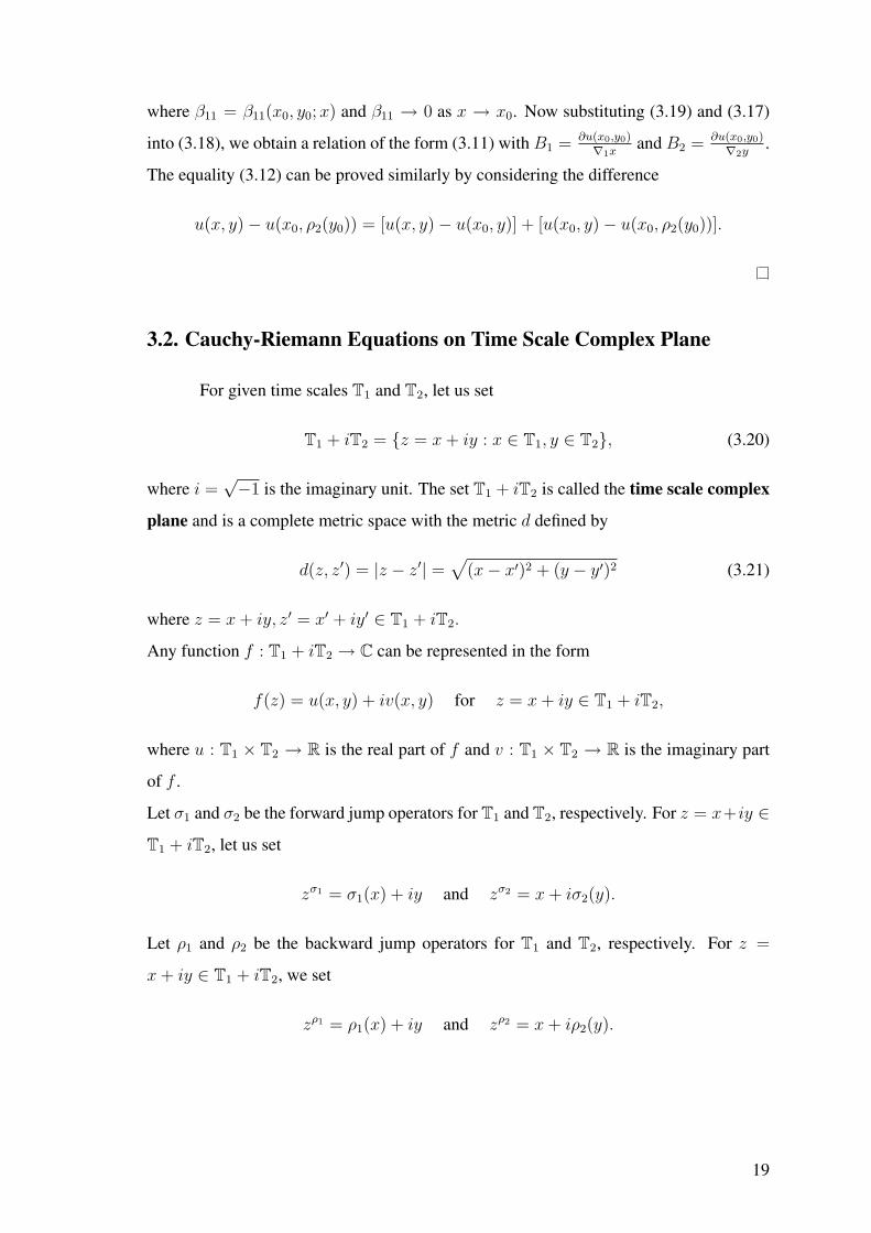
3.2. Cauchy-Riemann Equations on Time Scale Complex Plane

For given time scales T1 and T2, let us set

T1 + iT2 = {z = x + iy : x ∈ T1, y ∈ T2}, (3.20)

where i =√−1 is the imaginary unit. The set T1 + iT2 is called the time scale complex

plane and is a complete metric space with the metric d defined by

d(z, z′) = |z − z′| =√

(x− x′)2 + (y − y′)2 (3.21)

where z = x + iy, z′ = x′ + iy′ ∈ T1 + iT2.

Any function f : T1 + iT2 → C can be represented in the form

f(z) = u(x, y) + iv(x, y) for z = x + iy ∈ T1 + iT2,

where u : T1 × T2 → R is the real part of f and v : T1 × T2 → R is the imaginary part

of f .

Let σ1 and σ2 be the forward jump operators for T1 and T2, respectively. For z = x+iy ∈

T1 + iT2, let us set

zσ1 = σ1(x) + iy and zσ2 = x + iσ2(y).

Let ρ1 and ρ2 be the backward jump operators for T1 and T2, respectively. For z =

x + iy ∈ T1 + iT2, we set

zρ1 = ρ1(x) + iy and zρ2 = x + iρ2(y).

19

3.2.1. Delta Analytic Functions

Definition 25. A complex-valued function f : T1 + iT2 → C is delta differentiable (or

delta analytic) at a point z0 = x0 + iy0 ∈ Tκ1 + iTκ

2 if there exists a complex number A

(depending in general on z0) such that

f(z0)− f(z) = A(z0 − z) + α(z0 − z) (3.22)

f(zσ10 )− f(z) = A(zσ1

0 − z) + β(zσ10 − z) (3.23)

f(zσ20 )− f(z) = A(zσ2

0 − z) + γ(zσ20 − z) (3.24)

for all z ∈ Uδ(z0), where Uδ(z0) is a δ-neighborhood of z0 in T1 + iT2, α = α(z0, z),

β = β(z0, z) and γ = γ(z0, z) are defined for z ∈ Uδ(z0), they are equal to zero at z = z0,

and

limz→z0

α(z0, z) = limz→z0

β(z0, z) = limz→z0

γ(z0, z) = 0.

Then the number A is called the delta derivative (or ∆-derivative) of f at z0 and is

denoted by f∆(z0).

Theorem 26. Let the function f : T1 + iT2 → C have the form

f(z) = u(x, y) + iv(x, y) for z = x + iy ∈ T1 + iT2.

Then a necessary and sufficient condition for f to be ∆-differentiable (as a function of the

complex variable z) at the point z0 = x0 + iy0 ∈ Tκ1 + iTκ

2 is that the functions u and v be

completely ∆-differentiable (as a function of the two real variables x ∈ T1 and y ∈ T2)

at the point (x0, y0) and satisfied the Cauchy-Riemann equations

∂u

∆1x=

∂v

∆2yand

∂u

∆2y= − ∂v

∆1x(3.25)

at (x0, y0). If these equations are satisfied, then f∆(z0) can be represented in any of the

forms

f∆(z0) =∂u

∆1x+ i

∂v

∆1x=

∂v

∆2y− i

∂u

∆2y=

∂u

∆1x− i

∂u

∆2y=

∂v

∆2y+ i

∂v

∆1x, (3.26)

where the partial derivatives are evaluated at (x0, y0).

Proof. First we show necessity. Assume that f is ∆-differentiable at z0 = x0 + iy0 with

f∆(z0) = A. Then (3.22)-(3.24) are satisfied. Letting

f = u + iv, A = A1 + iA2, α = α1 + iα2, β = β1 + iβ2, γ = γ1 + iγ2,

20

we get from (3.22)-(3.24), equating the real and imaginary parts of both sides in each of

these equations,u(x0, y0)− u(x, y) = A1(x0 − x)− A2(y0 − y) + α1(x0 − x)− α2(y0 − y)

u(σ1(x0), y0)− u(x, y) = A1[σ1(x0)− x]− A2(y0 − y) + β1[σ1(x0)− x]− β2(y0 − y)

u(x0, σ2(y0))− u(x, y) = A1(x0 − x)− A2[σ2(y0)− y] + γ1(x0 − x)− γ2[σ2(y0)− y]

andv(x0, y0)− v(x, y) = A2(x0 − x)− A1(y0 − y) + α2(x0 − x)− α1(y0 − y)

v(σ1(x0), y0)− v(x, y) = A2[σ1(x0)− x]− A1(y0 − y) + β2[σ1(x0)− x]− β1(y0 − y)

v(x0, σ2(y0))− v(x, y) = A2(x0 − x)− A1[σ2(y0)− y] + γ2(x0 − x)− γ1[σ2(y0)− y]

Hence, taking into account that αj → 0, βj → 0, and γj → 0 as (x, y) → (x0, y0), we get

that the functions u and v are completely ∆-differentiable (as functions of the two real

variables x ∈ T1 and y ∈ T2) and that

A1 =∂u(x0, y0)

∆1x, −A2 =

∂u(x0, y0)

∆2y, A2 =

∂v(x0, y0)

∆1x, A1 =

∂v(x0, y0)

∆2y.

Therefore the Cauchy-Riemann equations (3.25) hold and we have the formulas (3.26).

Now we show sufficiency. Assume that the functions u and v, where f = u +

iv, are completely ∆-differentiable at the point (x0, y0) and that the Cauchy-Riemann

equations (3.25) hold. Then we haveu(x0, y0)− u(x, y) = A′

1(x0 − x)− A′2(y0 − y) + α′1(x0 − x)− α′2(y0 − y)

u(σ1(x0), y0)− u(x, y) = A′1[σ1(x0)− x]− A′

2(y0 − y) + β′11[σ1(x0)− x]− β′12(y0 − y)

u(x0, σ2(y0))− u(x, y) = A′1(x0 − x)− A′

2[σ2(y0)− y] + β′21(x0 − x)− β′22[σ2(y0)− y]

andv(x0, y0)− v(x, y) = A′′

1(x0 − x)− A′′2(y0 − y) + α′′1(x0 − x)− α′′2(y0 − y)

v(σ1(x0), y0)− v(x, y) = A′′1[σ1(x0)− x]− A′′

2(y0 − y) + β′′11[σ1(x0)− x]− β′′12(y0 − y)

v(x0, σ2(y0))− v(x, y) = A′′1(x0 − x)− A′′

2[σ2(y0)− y] + β′′21(x0 − x)− β′′22[σ2(y0)− y]

where α′j, β′ij and α′′j , β

′′ij tend to zero as (x, y) → (x0, y0) and

A′1 =

∂u(x0, y0)

∆1x=

∂v(x0, y0)

∆2y= A′′

2 =: A1

and

−A′2 = −∂u(x0, y0)

∆2y=

∂v(x0, y0)

∆1x= A′′

1 =: A2.

21

Therefore

f(z0)− f(z) = (A1 + iA2)(z0 − z) + α(z0 − z),

f(zσ10 )− f(z) = (A1 + iA2)(z

σ10 − z) + β(zσ1

0 − z),

f(zσ20 )− f(z) = (A1 + iA2)(z

σ20 − z) + γ(zσ2

0 − z),

where

α = (α′1 + iα′′1)x0 − x

z0 − z+ (α′2 + iα′′2)

y0 − y

z0 − z,

β = (β′11 + iβ′′11)σ1(x0)− x

zσ10 − z

+ (β′12 + iβ′′12)y0 − y

zσ10 − z

,

γ = (β′21 + iβ′′21)x0 − x

zσ20 − z

+ (β′22 + iβ′′22)σ2(y0)− y

zσ20 − z

.

Since

|α| ≤ |α′1 + iα′′1|∣∣∣∣x0 − x

z0 − z

∣∣∣∣ + |α′2 + iα′′2|∣∣∣∣y0 − y

z0 − z

∣∣∣∣≤ |α′1 + iα′′1|+ |α′2 + iα′′2| ≤ |α′1|+ |α′′1|+ |α′2|+ |α′′2|,

we have α → 0 as z → z0. Similarly, β → 0 and γ → 0 as z → z0. Consequently, f is

∆-differentiable at z0 and f∆(z0) = A1 + iA2.

Remark 27. (See (Bohner and Guseinov 2004)). If the functions u, v : T1×T2 → R are

continuous and have the first order partial delta derivatives ∂u(x,y)∆1x

, ∂u(x,y)∆2y

, ∂v(x,y)∆1x

, ∂v(x,y)∆2y

in some δ-neighborhood Uδ(x0, y0) of the point (x0, y0) ∈ Tκ1×Tκ

2 and if these derivatives

are continuous at (x0, y0), then u and v are completely ∆-differentiable at (x0, y0).

Therefore in this case, if in addition the Cauchy-Riemann equations (3.25) are satisfied,

then f(z) = u(x, y) + iv(x, y) is ∆-differentiable at z0 = x0 + iy0.

Example 28. (i) The function f(z) =constant on T1 + iT2 is ∆-analytic everywhere and

f∆(z) = 0.

(ii) The function f(z) = z on T1 + iT2 is ∆-analytic everywhere and f∆(z) = 1.

(iii) Consider the function

f(z) = z2 = (x + iy)2 = x2 − y2 + i2xy on T1 + iT2.

Hence u(x, y) = x2 − y2, v(x, y) = 2xy, and

∂u(x, y)

∆1x= x + σ1(x),

∂u(x, y)

∆2y= −y − σ2(y),

∂v(x, y)

∆1x= 2y,

∂v(x, y)

∆2y= 2x.

22

Therefore the Cauchy-Riemann equations become

x + σ1(x) = 2x and − y − σ2(y) = −2y,

which hold simultaneously if and only if σ1(x) = x and σ2(y) = y simultaneously. It

follows that the function f(z) = z2 is not ∆-analytic at each point of Z + iZ. So, the

product of two ∆-analytic functions need not be ∆-analytic.

(iv) The function f(z) = x2 − y2 + i(2xy + x + y) is ∆-analytic everywhere on Z + iZ.

Since, Cauchy-Riemann equations are satisfied:

∂u(x, y)

∆1x= x + σ1(x) = 2x + 1,

∂u(x, y)

∆2y= −y − σ2(y) = −2y − 1,

∂v(x, y)

∆1x= 2y + 1,

∂v(x, y)

∆2y= 2x + 1.

This function is not analytic anywhere on R + iR = C.

(v) The function f(z) = x2 − y2 + i3xy is ∆-analytic everywhere on T + iT where

T = {2n : n ∈ Z} ∪ {0}.

Since, Cauchy-Riemann equations are satisfied:

∂u(x, y)

∆1x= x + σ1(x) = 3x =

∂v(x, y)

∆2y,

∂u(x, y)

∆2y= −y − σ2(y) = −3y = −∂v(x, y)

∆1x.

Remark 29. (i) If T1 = T2 = R, then T1 + iT2 = R+ iR = C is the usual complex plane

and the three condition (3.22)-(3.24) of Definition 25 coincide and reduce to the classical

definition of analyticity (differentiability) of functions of a complex variable.

(ii) Let T1 = T2 = Z. Then T1 + iT2 = Z + iZ = Z[i] is the set of Gaussian integers.

The neighborhood Uδ(z0) of z0 contains the single point z0 for δ < 1. Therefore, in this

case, the condition (3.22) disappears, while the conditions (3.23) and (3.24) reduce to the

single conditionf(z0 + 1)− f(z0)

1=

f(z0 + i)− f(z0)

i(3.27)

with f∆(z0) equal to the left (and hence also to the right) hand side of (3.27). The condi-

tion (3.27) coincides with the condition of forward monodiffric functions in (2.5).

(iii) If T1 = R and T2 = hZ = {hk : k ∈ Z} where h > 0, then (3.22) and (3.23)

coincide and in any of them, dividing both sides by (z0 − z) where z = x + ikh and

23

z0 = x0 + ik0h, and taking limit as z → z0 (which just means x → x0), with k = k0 we

have

limx→x0

f(x0 + ik0h)− f(x + ik0h)

x0 − x= A.

Similarly by (3.24) we getf(z0 + ih)− f(z)

ih= A.

Equating this two results gives the condition of forward semi-discrete analytic functions:

∂f(z)

∂x= [f(z + ih)− f(z)]/ih, z = x + ikh.

Remark 30. We can combine Cauchy-Riemann equations for delta analytic functions in

one complex equation as follows:

∂f

∆1x=

1

i

∂f

∆2y(3.28)

(i) If T1 = T2 = R, then we have

∂f

∂x=

1

i

∂f

∂y

∂u

∂x+ i

∂v

∂x=

1

i

(∂u

∂y+ i

∂v

∂y

)Equating real and imaginary parts, we get the usual Cauchy-Riemann equations:

∂u

∂x=

∂v

∂yand

∂u

∂y= −∂v

∂x.

(ii) If we take T1 = T2 = Z then the equation (3.28) becomes

∆xf =1

i∆yf

which is exactly the condition for forward monodiffric functions

f(z + 1)− f(z)

1=

f(z + i)− f(z)

i.

(iii) With T1 = R and T2 = hZ, the equation (3.28) becomes

∂f

∂x=

1

i

f(z + ih)− f(z)

h.

which is the equation for forward semi-discrete analytic functions.

24

3.2.2. Nabla Analytic Functions

Definition 31. A complex-valued function f : T1 + iT2 → C is nabla differentiable (or

nabla analytic) at a point z0 = x0 + iy0 ∈ T1κ + iT2κ if there exists a complex number B

(depending in general on z0) such that

f(z)− f(z0) = B(z − z0) + α(z − z0) (3.29)

f(z)− f(zρ1

0 ) = B(z − zρ1

0 ) + β(z − zρ1

0 ) (3.30)

f(z)− f(zρ2

0 ) = B(z − zρ2

0 ) + γ(z − zρ2

0 ) (3.31)

for all z ∈ Uδ(z0), where Uδ(z0) is a δ-neighborhood of z0 in T1 + iT2, α = α(z0, z),

β = β(z0, z) and γ = γ(z0, z) are defined for z ∈ Uδ(z0), they are equal to zero at z = z0,

and

limz→z0

α(z0, z) = limz→z0

β(z0, z) = limz→z0

γ(z0, z) = 0.

Then the number B is called the nabla derivative (or ∇-derivative) of f at z0 and is

denoted by f∇(z0).

Theorem 32. Let the function f : T1 + iT2 → C have the form

f(z) = u(x, y) + iv(x, y) for z = x + iy ∈ T1 + iT2.

Then a necessary and sufficient condition for f to be ∇-differentiable (as a function of

the complex variable z) at the point z0 = x0 + iy0 ∈ T1κ + iT2κ is that the functions u

and v be completely ∇-differentiable (as a function of the two real variables x ∈ T1 and

y ∈ T2) at the point (x0, y0) and satisfied the Cauchy-Riemann equations

∂u

∇1x=

∂v

∇2yand

∂u

∇2y= − ∂v

∇1x(3.32)

at (x0, y0). If these equations are satisfied, then f∇(z0) can be represented in any of the

forms

f∇(z0) =∂u

∇1x+ i

∂v

∇1x=

∂v

∇2y− i

∂u

∇2y=

∂u

∇1x− i

∂u

∇2y=

∂v

∇2y+ i

∂v

∇1x, (3.33)

where the partial derivatives are evaluated at (x0, y0).

Proof. Let us first show necessity. Assume that f is ∇-differentiable at z0 = x0 + iy0

with f∇(z0) = B. Then (3.29)-(3.31) are satisfied. Letting

f = u + iv, B = B1 + iB2, α = α1 + iα2, β = β1 + iβ2, γ = γ1 + iγ2,

25

we get from (3.29)-(3.31), equating the real and imaginary parts of both sides in each of

these equations,u(x, y)− u(x0, y0) = B1(x− x0)−B2(y − y0) + α1(x− x0)− α2(y − y0)

u(x, y)− u(ρ1(x0), y0) = B1[x− ρ1(x0)]−B2(y − y0) + β1[x− ρ1(x0)]− β2(y − y0)

u(x, y)− u(x0, ρ2(y0)) = B1(x− x0)−B2[y − ρ2(y0)] + γ1(x− x0)− γ2[y − ρ2(y0)]

andv(x, y)− v(x0, y0) = B2(x− x0)−B1(y − y0) + α2(x− x0)− α1(y − y0)

v(x, y)− v(ρ1(x0), y0) = B2[x− ρ1(x0)]−B1(y − y0) + β2[x− ρ1(x0)]− β1(y − y0)

v(x, y)− v(x0, ρ2(y0)) = B2(x− x0)−B1[y − ρ2(y0)] + γ2(x− x0)− γ1[y − ρ2(y0)]

Hence, taking into account that αj → 0, βj → 0, and γj → 0 as (x, y) → (x0, y0), we get

that the functions u and v are completely ∇-differentiable (as functions of the two real

variables x ∈ T1 and y ∈ T2) and that

B1 =∂u(x0, y0)

∇1x, −B2 =

∂u(x0, y0)

∇2y, B2 =

∂v(x0, y0)

∇1x, B1 =

∂v(x0, y0)

∇2y.

Therefore the Cauchy-Riemann equations (3.32) hold and we have the formulas (3.33).

Now we show sufficiency. Assume that the functions u and v, where f = u +

iv, are completely ∇-differentiable at the point (x0, y0) and that the Cauchy-Riemann

equations (3.32) hold. Then we haveu(x, y)− u(x0, y0) = B′

1(x− x0)−B′2(y − y0) + α′1(x− x0)− α′2(y − y0)

u(x, y)− u(ρ1(x0), y0) = B′1[x− ρ1(x0)]−B′

2(y − y0) + β′11[x− ρ1(x0)]− β′12(y − y0)

u(x, y)− u(x0, ρ2(y0)) = B′1(x− x0)−B′

2[y − ρ2(y0)] + β′21(x− x0)− β′22[y − ρ2(y0)]

andv(x, y)− v(x0, y0) = B′′

1 (x− x0)−B′′2 (y − y0) + α′′1(x− x0)− α′′2(y − y0)

v(x, y)− v(ρ1(x0), y0) = B′′1 [x− ρ1(x0)]−B′′

2 (y − y0) + β′′11[x− ρ1(x0)]− β′′12(y − y0)

v(x, y)− v(x0, ρ2(y0)) = B′′1 (x− x0)−B′′

2 [y − ρ2(y0)] + β′′21(x− x0)− β′′22[y − ρ2(y0)]

where α′j, β′ij and α′′j , β

′′ij tend to zero as (x, y) → (x0, y0) and

B′1 =

∂u(x0, y0)

∇1x=

∂v(x0, y0)

∇2y= B′′

2 =: B1

and

−B′2 = −∂u(x0, y0)

∇2y=

∂v(x0, y0)

∇1x= B′′

1 =: B2.

26

Therefore

f(z)− f(z0) = (B1 + iB2)(z − z0) + α(z − z0),

f(z)− f(zρ1

0 ) = (B1 + iB2)(z − zρ1

0 ) + β(z − zρ1

0 ),

f(z)− f(zρ2

0 ) = (B1 + iB2)(z − zρ2

0 ) + γ(z − zρ2

0 ),

where

α = (α′1 + iα′′1)x− x0

z − z0

+ (α′2 + iα′′2)y − y0

z − z0

,

β = (β′11 + iβ′′11)x− ρ1(x0)

z − zρ1

0

+ (β′12 + iβ′′12)y − y0

z − zρ1

0

,

γ = (β′21 + iβ′′21)x− x0

z − zρ2

0

+ (β′22 + iβ′′22)y − ρ2(y0)

z − zρ2

0

.

Since

|α| ≤ |α′1 + iα′′1|∣∣∣∣x− x0

z − z0

∣∣∣∣ + |α′2 + iα′′2|∣∣∣∣y − y0

z − z0

∣∣∣∣≤ |α′1 + iα′′1|+ |α′2 + iα′′2| ≤ |α′1|+ |α′′1|+ |α′2|+ |α′′2|,

we have α → 0 as z → z0. Similarly, β → 0 and γ → 0 as z → z0. Consequently, f is

∇-differentiable at z0 and f∇(z0) = B1 + iB2.

Remark 33. (See Theorem 23) If the functions u, v : T1 × T2 → R are continuous

and have the first order partial delta derivatives ∂u(x,y)∇1x

, ∂u(x,y)∇2y

, ∂v(x,y)∇1x

, ∂v(x,y)∇2y

in some

δ-neighborhood Uδ(x0, y0) of the point (x0, y0) ∈ T1κ × T2κ and if these derivatives are

continuous at (x0, y0), then u and v are completely∇-differentiable at (x0, y0). Therefore

in this case, if in addition the Cauchy-Riemann equations (3.32) are satisfied, then f(z) =

u(x, y) + iv(x, y) is ∇-differentiable at z0 = x0 + iy0.

Example 34. (i) Similar to the delta case, the functions f(z) =constant and g(z) = z on

T1 + iT2 are ∇-analytic everywhere with f∇(z) = 0 and g∇(z) = 1.

(ii) It is obvious that the function

f(z) = z2 = (x + iy)2 = x2 − y2 + i2xy on T1 + iT2

is not ∇-analytic at each point of Z + iZ by the same reason as the delta case.

(iii) The function f(z) = x2 − y2 + i(2xy − x− y) is ∇-analytic everywhere on Z + iZ.

Since, Cauchy-Riemann equations are satisfied:

∂u(x, y)

∇1x= x + ρ1(x) = 2x− 1,

∂u(x, y)

∇2y= −y − ρ2(y) = −2y + 1,

27

∂v(x, y)

∇1x= 2y − 1,

∂v(x, y)

∆2y= 2x− 1.

Note that this function is not delta analytic on Z + iZ

(iv) The function f(z) = x2 − y2 + i3xy is not ∇-analytic on T + iT where T = {2n :

n ∈ Z} ∪ {0}.

Since, Cauchy-Riemann equations are not satisfied:

∂u(x, y)

∇1x= x + ρ1(x) =

3x

26= 3x =

∂v(x, y)

∇2y,

∂u(x, y)

∇2y= −y − ρ2(y) = −3y

26= −3y =

∂v(x, y)

∇2y.

Note that this function is delta analytic everywhere on T + iT with the same T.

Remark 35. (i) If T1 = T2 = R, then T1 + iT2 = R+ iR = C is the usual complex plane

and the three condition (3.29)-(3.31) of Definition 31 coincide and reduce to the classical

definition of analyticity (differentiability) of functions of a complex variable.

(ii) Let T1 = T2 = Z. Then T1 + iT2 = Z + iZ = Z[i] is the set of Gaussian integers.

The neighborhood Uδ(z0) of z0 contains the single point z0 for δ < 1. Therefore, in this

case, the condition (3.29) disappears, while the conditions (3.30) and (3.31) reduce to the

single conditionf(z0)− f(z0 − 1)

1=

f(z0)− f(z0 − i)

i(3.34)

with f∇(z0) equal to the left (and hence also to the right) hand side of (3.34). The condi-

tion (3.34) coincides with the definition of backward monodiffric functions we defined in

(2.7).

(iii) If T1 = R and T2 = hZ = {hk : k ∈ Z} where h > 0, then (3.29) and (3.30)

coincide and in any of them, dividing both sides by (z − z0) where z = x + ikh and

z0 = x0 + ik0h, and taking limit as z → z0 (which just means x → x0), with k = k0 we

have

limx→x0

f(x0 + ik0h)− f(x + ik0h)

x0 − x= B.

Similarly by (3.31) we getf(z)− f(z − ih)

ih= B.

Equating this two results gives the condition of backward semi-discrete analytic functions

defined in (2.10).

28

Remark 36. We can combine Cauchy-Riemann equations for nabla analytic functions in

one equation as follows:∂f

∇1x=

1

i

∂f

∇2y(3.35)

(i) If T1 = T2 = R, then we have

∂f

∂x=

1

i

∂f

∂y

∂u

∂x+ i

∂v

∂x=

1

i

(∂u

∂y+ i

∂v

∂y

)Equating real and imaginary parts, we get the usual Cauchy-Riemann equations:

∂u

∂x=

∂v

∂yand

∂u

∂y= −∂v

∂x.

(ii) If we take T1 = T2 = Z then the equation (3.35) becomes

∇xf =1

i∇yf

which is exactly the condition for backward monodiffric functions

f(z)− f(z − 1)

1=

f(z)− f(z − i)

i.

(iii) With T1 = R and T2 = hZ, the equation (3.35) becomes

∂f

∂x=

1

i

f(z)− f(z − ih)

h.

which is the equation for backward semi-discrete analytic functions.

29

CHAPTER 4

CONCLUSION

The history of the theory of complex functions begins at the end of sixteen

century. The study of discrete counterparts of complex functions on Z2 has a history of

more than sixty years. Further, the semi-discrete analog of complex functions was firstly

introduced by Kurowski in 1963.

After calculus of time scales was introduced by Hilger in 1988, many concepts in

continuous and discrete analysis was rapidly unified. Bohner and Guseinov were the first

who made the unification of the continuous and discrete complex analysis by time scales.

They defined completely delta differentiable functions, Cauchy-Riemann equations and

delta analytic functions on products of two time scales. They also introduced complex

line delta and nabla integrals along time scales curves, and obtain a time scale version

of the classical Cauchy integral theorem on union of horizontal and vertical line segments.

In this thesis, we worked on continuous, discrete and semi-discrete analytic

functions and developed completely∇-differentiability,∇-analytic functions on products

of two time scales, and Cauchy-Riemann equations for nabla case.

Our further study will be on complex integration and we will investigate the gen-

eralization of time scale version of Cauchy integral theorem.

30

REFERENCES

Atici, F.M. and Guseinov, G.Sh., 2002. “On Green’s functions and positive solutionsfor boundary value problems on time scales”, Journal of Computational and AppliedMathematics, Vol. 141 pp. 7599.

Bohner, M. and Guseinov, G.Sh., 2004. “Partial Differentiation on time scales”, Dynam.Systems Appl. Vol. 13, pp. 351-379.

Bohner, M. and Guseinov, G.Sh., 2005. “An Introduction to Complex Functions onProduct of Two Time Scales”, J. Difference Equ. Appl.

Bohner, M. and Peterson, A., 2001. Dynamic Equations on Time Scales: An Introductionwith Applications, (Birkhauser, Boston), Chapter 1.

Duffin, R.J., 1956. “Basic properties of discrete analytic functions”, Duke Math. J., Vol.23, pp. 335-363.

Ferrand, J., 1944. “Fonctions preharmoniques et fonctions preholomorphes”, Bull. Sci.Math. Vol. 68, second series, pp. 152-180.

Guseinov, G.Sh., 2003. “Integration on time scales”, J. Math. Anal. Appl. Vol. 285, pp.107-127.

Helmbold, R.L., “Semi-discrete potential theory”, Carnegie Institute of Technology,Technical Report No. 34, DA-34-061-ORD-490, Office of Ordnance Research, U.S.Army.

Hilger, S., 1997. “Differential and difference calculus — unified.”, Nonlinear Analysis,Theory, Methods and Applications, Vol. 30, pp. 2683-2694.

Isaacs, R.P., 1941. “A finite difference function theory”, Univ. Nac. Tucuman Rev., Vol. 2,pp. 177-201.

Kiselman, C.O., 2005. “Functions on discrete sets holomorphic in the sense of Isaacs, ormonodiffric functions of the first kind”, Science in China, Ser. A Mathematics, Vol. 48Supp. 1-11.

Kurowski, G.J., 1963. “Semi-Discrete Analytic Functions”, Transaction of the AmericanSociety, Vol. 106, No. 1, pp. 1-18.

Kurowski, G.J., 1966. “Further results in the theory of monodiffric functions”, PasificJournal of Mathematics, Vol. 18, No. 1.

31