1

Analytical and Experimental Evaluation of Digital Control Systems for the Semi-Span Super-Sonic Transport (S4T) Wind Tunnel Model

Carol Wieseman*

NASA-Langley Research Center, Hampton, VA, 23681-2199 USA

David Christhilf † Lockheed Martin Services Inc, Civil-Exploration and Science, Hampton, VA 23681-2199 USA

Boyd Perry, III‡

NASA-Langley Research Center, Hampton, VA, 23681-2199 USA An important objective of the Semi-Span Super-Sonic Transport (S4T) wind tunnel model program was the demonstration of Flutter Suppression (FS), Gust Load Alleviation (GLA), and Ride Quality Enhancement (RQE). It was critical to evaluate the stability and robustness of these control laws analytically before testing them and experimentally while testing them to ensure safety of the model and the wind tunnel. MATLAB based software was applied to evaluate the performance of closed-loop systems in terms of stability and robustness. Existing software tools were extended to use analytical representations of the S4T and the control laws to analyze and evaluate the control laws prior to testing. Lessons were learned about the complex wind-tunnel model and experimental testing. The open-loop flutter boundary was determined from the closed-loop systems. A MATLAB/Simulink Simulation developed under the program is available for future work to improve the CPE process. This paper is one of a series of that comprise a special session, which summarizes the S4T wind-tunnel program.

Nomenclature

CLO = control law output CPE = controller performance evaluation FRF = frequency response function or frequency responses det = determinant G = open-loop plant FLAP = wing trailing edge control surface FLAPCOM = command to FLAP FLAPEXC = excitation to FLAP HT = horizontal tail HTCOM = command to HT HTEXC = excitation to HT IBMID15I = accelerometer located on the inboard middle section of the wing LTI = linear time invariant state-space representation of a system. MIMO = multi-input multi-output NIBAFTZ = nacelle inboard aft accelerometer in the z direction ! = dynamic pressure, psf RCV = ride control vane SISO = single-input single-output !! = time history of ith excitation to control surface !! = time history of ith control law output !! = time history of ith plant output !! = matrix of frequency responses of control law outputs to excitations !! = matrix of frequency responses of plant outputs to excitations σ = singular value

Subscripts f = flutter

*  Aerospace  Engineer,  Aeroelasticity  Branch,  Mail  Stop  340,  Associate  Fellow  AIAA  †  Research  Engineer  Staff,  Langley  Program  Office,  c/o  NASA_LaRC,  Mail  Stop  308,  Senior  Member  AIAA  ‡  Assistant  Branch  Head,  Aeroelasticity  Branch,  Mail  Stop  340,  Senior  Member  AIAA  

2

I. Introduction

The Semi-Span Super-Sonic Transport (S4T) wind-tunnel model was tested in the NASA Langley Transonic Dynamics Tunnel (TDT)1-3 under the auspices of the Supersonics Project/Fundamental Aeronautics Program. The S4T is a sophisticated, aeroelastically-scaled semispan wind-tunnel model based on the Technology Concept Aircraft (TCA) configuration, one of the configurations of the NASA High Speed Research Program of the 1990s. The unique structural configuration of supersonic transport aircraft combined with non-linear aerodynamics and rigid-body effects often results in highly complex nonlinear aeroelastic and/flight dynamic phenomenon. Active controls may be required on a future Supersonics Transport to achieve the required stability margins and performance of the aircraft throughout the flight envelope.

The S4T wind-tunnel model is equipped with three active control surfaces: (a fully moveable ride control vane (RCV) located near the pilot station; a wing trailing edge control surface (FLAP); and a fully moveable horizontal tail (HT) and flow-through nacelles with flexible mounts.4 The model was designed so that it would flutter within the TDT range of operation. The wind-tunnel model was heavily instrumented with accelerometers, unsteady pressure sensors, and strain gauges. A schematic of the instrumentation of the S4T wind-tunnel model is shown in Figure 1.

There were four wind-tunnel tests performed between 2007 and 2010. The first two tests were open-loop tests. The last two tests employed active control laws for Flutter Suppression (FS), Gust Load Alleviation (GLA), and Ride Quality Enhancement (RQE). Two objectives of the first two wind-tunnel tests were to understand the wind-tunnel model and to develop state-space representations of the wind-tunnel model for use in subsequent control law design and implementation in a MATLAB/Simulink simulation developed as part of the S4T program5. Control law designers used the data acquired and processed during these two open-loop tests to select suitable sensor/control-effector pairs.

During the first test, two configurations were tested: a nominal configuration and ballasted configuration.4 The ballasted configuration includes a greater engine weight and decreased pylon stiffness. The only model that was tested with active controls was the ballasted configuration.

A primary objective of the last two wind-tunnel tests was to assess the performance of several multi-objective control laws. During the third wind-tunnel entry FS, GLA, and RQE, control laws were tested below the open-loop flutter boundary. During the fourth wind-tunnel test, the best FS control laws from the third test were tested above the open-loop flutter boundary. The FS metric for the S4T program was 44% in flutter dynamic pressure. This metric was unable to actually be tested because of the first concern for model safety.

This paper addresses the use of MATLAB-based software called Controller Performance Evaluation (CPE). This software has been described before 6-7. CPE has been used for active controls tests in the Transonic Dynamics Tunnel including: Active Flexible Wing (AFW)6; Benchmark Active Controls Test (BACT)8-9; Piezoelectric

Figure 1. Model Instrumentation layout

3

Aeroelastic Response Tailoring Investigation (PARTI)10; and Actively Controlled Reduction of Buffet Affected Tails (ACROBAT) 11. The S4T program provided another opportunity to use CPE.

New capabilities have been added to CPE for the S4T and are discussed. Employing transfer matrices and calculations of the maximum and minimum singular values of the return difference matrix, CPE predicts the stability and robustness of multi-input/multi-output closed-loop (in the present case, aeroservoelastic) systems.

With the loops open, CPE can predict the stability and robustness of the closed-loop system, affording test engineers the opportunity to avoid, by not closing the loops, an unexpected, and perhaps catastrophic, closed-loop instability. With the loops closed, CPE can determine the stability and robustness of the closed-loop system in near-real time and can also simultaneously predict the stability of the open-loop system. Thus, with this latter capability, test engineers can ascertain the open-loop flutter boundary while safely testing closed loop.

A review of the overall CPE concept is presented, followed by a review of the theory supporting it. Next, a discussion of the various types of input signals used by CPE is offered, followed by a description of the several options of CPE employed over the course of the project. Finally, a number of results are presented, illustrating, on the one hand, the usefulness and versatility of CPE, and, on the other hand, questions and issues regarding uncertainties associated with the choice of processing parameters, signal-to-noise ratios, excitation signals and excitation amplitude.

II. Controller Performance Evaluation (CPE) Process for S4T

The CPE process for the S4T wind-tunnel model involved four steps:

Step 1 – Control Law Screening

This first step was performed before actual wind-tunnel testing began. It involved evaluating the stability and robustness of the closed-loop system using analytical models of the wind-tunnel model (the “plant”). Continuous state-space analytical models of the plant and candidate control laws were used to calculate the necessary frequency responses to perform the stability and robustness calculations. (This process of using analytical models only was called “analytical CPE.”) If the closed-loop system employing a particular control law showed sufficient robustness margins throughout the expected wind-tunnel testing envelope, then the decision was made to accept that control law for testing

Step 2 – Control Law Verification

For those control laws that passed the screening step, the next step involved loading the control laws into the actual digital control computer that would be used during wind-tunnel testing and performing checks to assure that this loaded control law was loaded correctly.

Step 3 – Stability and Robustness Using Open-Loop Time Histories

This step was performed during wind-tunnel testing at a nominal subcritical wind-on condition. A particular control law was loaded into the digital control computer and was operating (that is, it was receiving sensor signals and outputting control surface commands), but all control loops of the control law were open at points prior to the summing junctions, as depicted in figure 2. Inputs, !!, were applied to each plant input and recorded and plant outputs, !!, and control law outputs, !!, were recorded. Frequency response functions of the plant and control law were obtained from these time records and the CPE process was executed, predicting the closed-loop system stability and robustness while all loops were open. If the control law was predicted to destabilize the system or if there were inadequate robustness margins predicted, the control law would not be tested closed-loop. If there were adequate robustness margins indicated, the loops would be closed and closed-loop testing for this particular control law would begin. This step is referred to as “Open-Loop CPE.”

Step 4 – Stability and Robustness Using Closed-Loop Time Histories

The initial closed-loop stability and robustness determinations were made at the same wind-tunnel conditions as in Step 3 – nominal, subcritical, wind-on – but all loops of the particular control law were now closed, as depicted in figure 3. The same operations outlined in Step 3 were now repeated: Inputs, !!, are applied to each plant input and recorded and plant outputs, !!, and control law outputs, !!, are recorded. Frequency response functions of the plant and control law were obtained and the CPE process was executed, determining now the closed-loop system stability and robustness while all loops are closed. If there were adequate robustness margins determined, the next

4

test condition would be attained by increasing the dynamic pressure at constant Mach number and the CPE process would be repeated and new robustness margins determined. This sequence of increasing dynamic pressure and executing the CPE process to ascertain if robustness margins were adequate was repeated until the margins were no longer adequate. This step is referred to as “Closed-Loop CPE.”

III. Controller Performance Evaluation Theory

The equations, theory and details are presented in the references6-7 and are repeated here to assist in

understanding results that will be presented. The block diagrams of the controller-plant system are shown in Figure 2 and 3, depicting the open-loop and closed-loop systems, respectively with external excitations applied to the control surfaces.

Stability is evaluated by looking at plots of:

!"# ! + !" (1) where I+HG is the return difference matrix at the plant input point or the controls. For a single-input single-output (SISO) system this corresponds to a Nyquist plot where the critical point has been moved from -1,0 to the origin. This plot will be referred to as either “the determinant plot” or “the generalized Nyquist plot.”

If the system is open loop, the plant, G, and the controller, H, are, of course, both stable. For such a circumstance we are interested in employing the determinant plot to determine if, when the loops are closed, the closed-loop system will be stable or unstable. If the closed-loop system will be stable, there will be no encirclement of the critical point. On the other hand, a clockwise encirclement of the critical point would indicate that if the loop was closed, the closed-loop system would be unstable. Such a control law would be destabilizing and would not be tested.

If the system is closed-loop, the closed-loop system is in a stable condition. For such a circumstance we are interested in employing the determinant plot to determine if, were the loops to be opened, would the open-loop system be stable or unstable. The lack of a counter clockwise encirclement indicates that the open-loop plant is stable. A counter-clockwise encirclement of the critical point indicates that the open-loop plant would be unstable if the loops were opened.

In CPE, several variations of robustness are calculated and observed. These are the robustnesses with respect to multiplicative uncertainties at the plant input and plant output:

!!" ! = !!"# ! +!" ! (2)

!!" ! = !!"# ! + !" ! (3)  

and robustness with respect to an additive uncertainty:

Figure 3. Block diagram of closed-loop system with negative feedback

Figure 2. Block diagram of open-loop system

5

!! ! = !!!"# ! !!!" !! !

(4)  

The quantities ! + !" and ! + !" are the return difference matrices at the plant input and plant output points

respectively. The results of open-loop CPE and closed-loop CPE each yield the stability and robustness of the closed-loop system.

The frequency responses used to evaluate stability and robustness (shown in equations 1-4) are calculated using the analytical representations of the model and the control law prior to wind-tunnel testing (step 1) or from time histories generated using the MATLAB/Simulink simulation5 or obtained during wind-tunnel testing (steps 3-4).

If time histories are used, the matrices required in equations 1-4 are generated using the equations found in Table 1. Equations 5 a-d are the equations for an open-loop system. Equations 6 a-d are the equations for the closed-loop system. !! is the matrix of frequency responses of all the control law outputs to excitations at the controls side. !!  is the matrix of frequency responses of all the sensors with respect to the excitations applied to the control surfaces. Reference 7 provides details for when the excitations are applied at the sensors instead of the control side, which is an option when the number of sensors is greater than the number of control surfaces. This option wasn’t needed during the S4T tests and therefore is not presented in this paper.

Table 1 Basic CPE matrix equations, all matrices are a function of ω .

Open Loop Closed loop !       =    !! (5a) !       =   1 − !!! !!!!! ! (6a) !" =  !! (5b)   !" =   1 − !!! !!!!! ! (6b) !       =   !!!!! !! !!!!! ! (5c) !       =   !!!!! !! !!!!! ! (6c) !" =  ! ∙ ! (5d) !" =  ! ∙ ! (6d)

A sample CPE quad plot generated during wind-tunnel testing is shown in Figure 4. This case happens to be an open-loop condition at Mach 0.95, Q 42 psf. The control law operating was a MIMO control law with two inputs and two outputs. The upper two plots correspond to the robustness to multiplicative uncertainties, equations 2 and 3, respectively. The lower left is the robustness to additive uncertainties (equation 4). The lower right is the generalized Nyquist plot (equation 1). These quad plots are generated near real-time after acquiring the time histories. By examining the generalized Nyquist plot in Figure 4 it can be seen that since there is no encirclement of the critical point, the closed-loop system would be stable when the loop was closed. Even though this looks likes a Nyquist plot for a SISO system, determining gain and phase margins can be misleading for a MIMO system therefore requires looking at the robustness measures shown in other three plots.

The upper left plot has two curves because there are two control surfaces used for feedback with this MIMO control law. The lower curve gives an indication of stability margin for uncertainties as defined at the controls. The upper right plot has two curves because the control law uses two sensors for feedback. The lower curve on that plot gives an indication of stability margin for uncertainties as defined at the sensors.

For the S4T tests, the test team chose 0.3 as the minimum acceptable value of the minimum singular values. If CPE predicted a value below 0.3 for either multiplicative uncertainty, closed-loop testing of that control law was either not begun or terminated if begun. The minimum singular values for this test condition are well above the acceptable minimum value of 0.3. This minimum singular value corresponds to approximately ±3 dB of gain margin (where with no change in phase) and ±18 degrees of phase margin (where there is no change in gain).

The lower left plot shows the reciprocal of only the maximum singular value associated with the controller gain at each frequency so only a single curve is present even for MIMO control laws. The minimum is approximately 0.5 g’s/degree which is satisfactory. Low values of additive uncertainty are indicative of excessive control surface activity or sensitivity to mischaracterization of the plant.

With both overall stability assured and the minimum robustness criterion satisfied, the loops of this control law would be safely closed.

IV. Stability and Robustness Calculations Using Analytical Models

Prior to wind-on testing, the analytical plant models were used in conjunction with the state-space models of the

control laws to assess the stability and robustness margins throughout the test envelope. The analytical plant models developed for the S4T were used for control law design and for a MATLAB/Simulink simulation5. The matrices

6

needed for the minimum singular value calculations and plots were therefore available from purely analytical models.

Five types of analytical plant models were created and are listed in Table 2. They are the Doublet Lattice

Method (DLM) and Wind Tunnel Based (WTB) models developed by M4 Engineering, Inc., the Finite Element Analysis (FEA) model developed by NASA and the ZONA Aerodynamics (ZAERO) and ZONA Euler Unsteady Solver (ZEUS) models developed by Zona Technologies. M4 Engineering12-13 and Zona Technologies14-16 were NASA Research Announcement (NRA) partners working under contract to develop control laws for the S4T. M4 updated the finite element model incorporating data from early wind-off stress and loads tests to improve the finite element model. The WTB model had the frequencies tuned to GVT tests. The DLM and WTB were residualized with imbedded actuators so it was not feasible to change the actuators in these models. The FEA model developed by NASA used the latest finite element model from M4, modal damping of 0.25% and did not include actuators. The subsonic aerodynamics were Doublet Lattice and the supersonic aerodynamics were Zona51, both linear theories.

The ZAERO and ZEUS models were developed by the NRA partner Zona. The ZAERO model used linear aerodynamics and modal damping of 1%. The ZEUS models used the ZAERO models but the generalized aerodynamic forces that were used were calculated using Zona’s Euler Unsteady Aerodynamic, therefore incorporating non-linear aerodynamics. The ZAERO and ZEUS models included actuators. However due to their formulation, it was feasible to extract the actuators from the state-space models. The three actuators could then be linked in series to the LTI models that did not include actuators. The same actuator models could also be used once again with the ZAERO and ZEUS models, or they could be replaced with updated actuator models as needed. Details regarding the actuators and more details regarding the analytical models are provided in reference 17.

Figure 4. Sample CPE results for MIMO control law, M=0.95, Q=42 psf.

7

Each of the analytical models were different as reflected in the flutter dynamic pressures and frequencies shown in Table 3 and 4. The Mach numbers which were wind-tunnel tested are highlighted as shaded columns.

Both M4 and Zona compared frequency responses of their analytical models to experimental data showing reasonable or good correlation between their models at dynamic pressures up to approximately 62 psf.12,14 However because of the uncertainty of the accuracy of the plant models and how well they represented the physical wind-tunnel model, CPE was conducted with each control law with all of the plant models at the control law design Mach number.

Examples of CPE using frequency responses generated from the analytical models for both plant and control

law are shown for a MIMO control law at M=0.95 at two dynamic pressures – one below the analytical flutter boundary and the second above. The control law used for these analytical CPE results is a MIMO control law (Zona v448)17. This classic MIMO 2x2 control law uses the HT and the FLAP control surfaces, and the nacelle inboard aft accelerometer (NIBAFTZ) and the inboard mid wing accelerometer (IBMID15I). This MIMO control law is actually two SISO control laws working in parallel with each other with no cross-talk within the control law.

The analytical models used for this comparison are FEA and ZEUS. Since the flutter dynamic pressure for both analytical models at this Mach number are almost the same (shown in Table 3), one might expect very similar results. Typically direct comparisons between the models was not done, but to illustrate the differences in the plant models and the resulting CPE results, direct comparisons between the plant frequency responses and the results from

Table 2. Summary of analytical state-space models

Plant Model Mach = 0.8 Mach=0.95 M=1.10 Additional Info Doublet Lattice Method (DLM)

Q=0–350 at increments of 10 psf

Additional Mach numbers available 0.6, 1.2

Wind-Tunnel Based (WTB)

Q=0–150 at 10 psf increments

Q=0–150 at 10 psf increments

Q=0–150 at 10 psf increments

Finite Element Analysis (FEA)

Q=0 to 250 psf in 5 psf increments

Q=0 to 250 psf in 5 psf increments

Q=0 to 250 psf in 5 psf increments

Additional Mach numbers available: 0.6, 0.9, 1.2

ZONA Aero (ZAERO)

Q=20 – 257 (25 values)

ZONA Euler-UnSteady (ZEUS)

Q=20 – 257 (25 values)

Q=28 – 334 (23 values)

Q=37 – 448 (23 values)

Table 3. Flutter dynamic pressures for analytical models

Flutter Dynamic Pressure, psf Plant Model M=0.60 M=0.80 M=0.90 M=0.95 M=1.10 M=1.20 DLM 84.6 80.4 89.7 WTB 59.0 53.0 58.2 FEA 72.9 77.3 77.4 75.2 98.7 119.5 ZAERO 84.7 ZEUS 89.0 74.9 124.1

Table 4. Flutter frequencies for analytical models

Flutter Frequency, Hz Plant Model M=0.60 M=0.80 M=0.90 M=0.95 M=1.10 M=1.20 DLM 7.33 7.19 7.19 WTB 7.57 7.48 7.59 FEA 7.98 7.83 7.67 7.52 7.80 7.91 ZAERO 7.38 ZEUS 7.42 7.16 7.54

8

CPE are shown in this paper. The frequency range chosen for performing the analytical CPE was from 1 to 35 Hertz with 3000 points which corresponds to a frequency resolution of 0.0113 Hertz. One of the advantages of using analytical models is there is no restriction on the frequency range or resolution that are used to calculate the frequency responses.

The first set of results is at a subcritical condition at Mach 0.95, Q 70 psf which corresponds to a condition 7% below the analytical open-loop flutter boundaries. Although the frequency responses were calculated from 1-35 Hz, the plant frequency responses shown in Figures 5 – 6 and the resulting CPE results shown in figures 7-10 are shown for 3 – 15 Hz to more clearly show the differences in behavior and character in the flutter frequency range. The flutter mechanism for both analytical models is the coalescence of two low-frequency modes with the first mode at approximately 7.1 Hz going unstable and the companion mode becoming more damped. This flutter mechanism was shown using a dynamic pressure root locus shown in reference 17.

Figure 5 shows frequency responses of NIBAFTZ with respect to HTCOM at Mach 0.95, Q 70 psf. The plant frequency responses show noticeably different characteristics. The first modal frequency is approximately 7.1 Hz. For the ZEUS model the first mode is much more pronounced and the second mode is barely visible. For the FEA model, both modes are visible and the second mode is somewhat more pronounced than the first. Larger amplitude peaks tend to be associated with low damping for a particular mode. For this sensor and actuator pair, the FEA model is not yet dominated by the low damping of the flutter mode as the open-loop plant heads toward instability.

Figure 6 shows frequency responses for the same plant models but a different sensor-control surface pair at the same Mach and dynamic pressure. For this case, the ZEUS model shows response at both the first and the second modal frequencies but the lower frequency mode still dominates. The FEA model appears to have a transfer function zero very close to the flutter frequency for this sensor-control surface pair resulting in a slight dip in the frequency response at approximately 7.2 Hz. The differences shown in these two figures have implications for control law design and control law evaluation because control law designers choose which sensor-control pairs to use based upon these kinds of plant frequency response characteristics.

Figures 7-10 show quad plots comparing the CPE results for these two plant models with the same MIMO control law. Figure 10 shows the determinant of the return difference matrix at the plant input (which is exactly the same as the determinant of the return difference matrix at the plant output). The determinant plot shows for this MIMO system that closing the loop for this open-loop stable system will not destabilize the plant because there is no encirclement of the critical point at the origin.

Figure 7 shows the robustness with respect to multiplicative uncertainties at the controls or plant inputs. There are four curves, two associated with each plant model because the MIMO control law has two control surfaces used for feedback. The lower curves for both plant models show good margins throughout the flutter frequency range. However the FEA model shows a singular value of approximately 0.3 at 13 Hz for this control law which indicates a sensitivity to increased control law gain at this frequency. In the context of an experimental test, it is important to monitor these minimum singular values as tunnel conditions change.

Figure 8 shows the robustness with respect to multiplicative uncertainties at the sensors or the plant outputs. As with Figure 7, the singular values for the ZEUS model look acceptably large throughout the entire frequency range. However for the FEA model, there are minimum singular values below 0.5 at both 13 Hz and approximately 8 Hz. It should be noted that this control law was designed with the ZEUS plant model and not the FEA model. The singular values in the flutter frequency range for all of the models can be expected to decrease as conditions approach the open-loop flutter boundary. Because the flutter mode is changing its characteristics as conditions cross the open-loop flutter boundary, the singular values in the flutter frequency range must be monitored closely with changing conditions. The minimum singular values at other frequencies must also be monitored because they could be adversely affected by the control law and they could be driven unstable.

Comparisons are also shown for dynamic pressures of 85 psf and 84 psf, for the FEA and the ZEUS models respectively, in Figure 11 - 16. These are dynamic pressure conditions of the analytical plant models that were available at this Mach number and correspond to dynamic pressures approximately 13% above their respective analytical flutter boundaries. For this post-critical condition, the companion mode can be expected to be highly damped and not evident in the frequency response plots whereas the flutter mode itself should dominate that frequency range. In Figure 11 it is interesting to note that the peak frequencies are noticeably different between the FEA and the ZEUS models. The FEA peak is at approximately 7.9 Hz and the ZEUS peak is at approximately 7.2 Hz. A similar difference in the frequencies of the peaks is shown in Figure 12 for a different sensor-control surface pair. A frequency mismatch such as shown in the figure is one kind of uncertainty that one can expect prior to testing, and control law designers need to consider these uncertainties when deciding their control law design strategy.

9

Figure 16 shows the determinant of the return difference matrix. For this control law, the determinant plot shows a counter clockwise encirclement of the critical point for both plant models. The large circle symbols are at approximately 7.6 Hz and the small circle symbols are at approximately 8.1 Hz for both curves. These symbols show the direction of the encirclement. Even from the determinant plot for this MIMO system, one might expect that the ZEUS plant model produces larger singular values than the FEA model because of the proximity of the FEA determinant plot curve to the critical point at the origin for a frequency between 7.6 and 8.1 Hz as indicated by the location of the symbols on the curve.

Figure 13 shows the minimum singular values for the ZEUS model are greater than 0.3 across the entire frequency range. The minimum singular values for the FEA model are less than 0.2 at approximately 7.9 Hz and 0.3 at 13 Hz. Similar observations apply to Figure 14. Figure 15 shows a minimum at approximately 0.32 g/deg at approximately 7.8 Hz when using the FEA plant. The ZEUS model doesn’t show any such potential gain sensitivity at that frequency. With the CPE results based on ZEUS model indicating adequate margins and the CPE results using the FEA model violating the screening criteria at this condition, it was decided to evaluate this control law experimentally open-loop using the singular values based on experimental data. Once open-loop CPE was conducted experimentally, the decision to close the loop and whether to continue to higher dynamic pressure was based strictly on the experimental results.

10

Figure 5 Comparison of NIBAFTZ/HTCOM frequency responses, below !!

Figure 6 Comparison of IBMID15I/FLAPCOM frequency responses, below !!.

Figure 7 Comparison of robustness with respect to multiplicative uncertainty at plant input, below !!.

Figure 8 Comparison of robustness with respect to multiplicative uncertainty at plant output, below !!.

Figure 9 Comparison of robustness to additive uncertainty, below Qf.

Figure 10 Comparison of determinant of return difference matrix, below Qf.

11

Figure 13 Comparison of robustness with respect to multiplicative uncertainty at plant input, above Qf.

Figure 14 Comparison of robustness with respect to multiplicative uncertainty at plant output, above Qf.

Figure 16 Comparison of determinant of return difference matrix, above Qf.

Figure 11 Comparison of NIBAFTZ/HTCOM frequency responses, above Qf.

Figure 12 Comparison of IBMID15I/FLAPCOM frequency responses, above Qf.

Figure 15 Comparison of robustness to additive uncertainty, above analytical flutter boundary. above Qf.

12

V. Controller Verification

Once the control laws have been prescreened

(step 1) and the decision has been made to test a control law with the wind-tunnel model, the loading of the control laws needed to be verified. Control law designers provided control laws to NASA as continuous MATLAB linear time invariant (LTI) objects. Control law verification was deemed necessary because NASA had to modify the control laws so that they would be compatible with the operating features of the digital control computer that would be used during wind-tunnel testing. The first modification was to “pad” the control laws, or increase their order from their original size to 40 states. This padding resulted in all control laws, regardless of their original order, having the same final order, which made implementation of all control laws on the digital control computer much easier. The second modification was to discretize each control law to the sample rate of the digital control computer.

Control law verification involves sending an excitation to each input of the control law and measuring the control law outputs. Frequency responses are calculated from these time histories and compared with frequency responses calculated using the analytical state-space models of the control laws. An example of wind-off controller verification is shown in Figure 17. Because of the close match in magnitude and phase of these plots, it is clear that the correct control law is loaded and is being executed. All control laws were required to pass this step.

VI. Stability and Robustness Using Experimental Time Histories – Open Loop Each control law was designed for a specific Mach number. On a given day of wind-tunnel testing a control

law would first be loaded and then verified as described previously and then the tunnel condition would be set to that Mach number at a dynamic pressure well below the open-loop flutter boundary. Open-loop CPE would be conducted. After confirming that the control law would not destabilize the model and there was satisfactory robustness, the loop would then be closed and closed-loop CPE was performed at the same condition.

In order to conduct CPE each of the control surfaces needed to be excited in order to obtain the frequency responses for calculating the stability and robustness of the closed-loop system. Previous tests that used CPE 5-10 used individual excitations applied to each control effector in sequence. The excitation used for the first two wind-tunnel tests for system identification and characterization was predominantly a log sweep (chirp) signal from 0.5 to 25 Hz. Each control surface was excited one at a time.

During the third and fourth S4T wind-tunnel tests (the active controls tests), the control surface used by a SISO control law was excited with a multisine excitation. For a MIMO control law, the two control surfaces were excited with multisine excitations either one at a time or simultaneously with orthogonal multisine excitations18. A multisine signal is a sum of sinusoid components with unique frequencies. Each multisine signal contains frequencies that no other multisine signal has so that all of the multisine signals are mutually orthogonal in both the time and frequency domains. Since the multisine signals are orthogonal to each other, the frequency responses can be calculated for each sensor with respect to each control surface independently using one pair of excitations sent to the model simultaneously therefore reducing test time. One advantage of multisine signals even for a single excitation as compared to a sine sweep, is that for a sine sweep there will be resonant frequencies for which the response amplitude will be large, which limits the allowable amplitude across all frequencies. In contrast, the multisine looks more like a random signal but with the advantage that it has uniform signal strength across the frequency range and is repeatable unlike a true random signal. Since there are no resonant peaks when using a multisine excitation, the amplitude of the excitation is not limited by the peaks. The uncertainty associated with using multisine excitations for analysis is a subject of current research under the Fundamental Aeronautics Program.19

Figure 17. Example of wind-off controller verification

13

For experimental CPE, specific excitation(s) were sent to the model and time histories of the excitation, model responses and control law outputs (CLO) were measured. The discrete frequencies of the signals used for constructing the multisine function do not correspond exactly with the frequencies of the processing of the time histories with the FRF processing parameters. The default processing parameters were a 4k block size, an overlap of 75% and a Hanning window which result in a frequency resolution of 0.2441 Hz.

During previous tests5-10 where CPE was used, these same processing parameters were and in most cases gave reasonable FRF estimates and frequency resolution. At locations far from the open-loop stability boundary these parameters are adequate. Near the open-loop flutter boundary the loop of the determinant that corresponds to the flutter mode becomes large and therefore the distance between the points for adjacent frequencies can be large and at times during S4T testing this resolution was not fine enough to ascertain the details of the behavior of the determinant. The data would also be processed with 16k and 8k blocksizes to attempt to ascertain a better understanding of the behavior of the determinant in the frequency range of the instability. Sometimes processing with larger block sizes was problematic as the FRF’s with the larger block size can be more noisy because of the reduced number of averages. The goal was to gain as much insight as possible from the limited data available.

Another technique implemented for the S4T was the use of presplining the FRF’s. The frequency responses that were calculated using the default processing parameters were splined using the MATLAB splining function prior to the singular value and determinant calculations. This is an area that warrants more thorough future investigation.

Performing open-loop and closed-loop CPE at the same conditions provides the opportunity to evaluate CPE uncertainty more closely. The CPE analysis for an open-loop and closed-loop system should give the same results, within the context of variability from one test point to the next for identical conditions. However there are slight differences as shown in Figure 18– 19 for this M=0.80 SISO control law, referred to as Zona v16 by the control law designer. In the determinant plot shown in Figure 18, the circle symbol is at approximately 7.6 Hz and the diamond symbol is at approximately 8.1 Hz. For this subcritical condition, the loop associated with the flutter mode is nominally aligned with the positive real axis by the design of this control law. The open-loop estimate shows a larger area inside the curve. Figure 19 shows the minimum singular values of the return difference matrix. The closed-loop results show less robustness at 7 Hz as compared to the open-loop analysis.

There are several possible reasons for these differences in the determinant and singular value plots. The return difference matrix used in the open-loop CPE results are frequency response estimates calculated directly from the time histories (equation 5b) whereas in the closed-loop system the return difference matrix is calculated by extraction from a closed loop system (equation 6b) which involves the calculation of two sets of frequency responses.

Another possible reason for differences is the impact of signal to noise ratio. The excitation amplitude typically was 0.3-0.4 degrees. A larger amplitude excitation would be desired in terms of increasing the signal to noise ratio, but concern for saturation of control surfaces, and overly exciting model dynamics were considerations which limited the amplitude of the excitation that could be used. The control law feedback can attenuate the command to the actuators which can also degrade the signal-to-noise ratio.

One of the aspects of CPE is the calculation of the open loop experimental plant, G, for an open-loop system (equation 5a), or the extraction of the open-loop plant from the closed-loop system (equation 6a). These experimental plant frequency responses were also saved and were used to perform CPE with a combination of experimentally derived plant frequency responses and FRFs from analytical state-space representation of other control laws than the one that was active at the time of the data was acquired.

14

VII. Experimental Open-Loop Flutter Boundary Estimation from Closed-Loop CPE.

For probing the open-loop flutter boundary at a particular Mach number, the typical procedure was to go to a subcritical dynamic pressure, close the control loop with a satisfactory control law then increase the dynamic pressure by bleeding in heavy gas at constant Mach number to go to a higher dynamic pressure. Stability and robustness margins would then be reevaluated to determine whether it was advisable to continue to higher dynamic pressure. This process would be stopped when margins were inadequate or the response to turbulence was excessive.

One of the key contributions of CPE is the determination of the experimental open-loop flutter boundaries from the closed-loop CPE results. The first step is to identify the presence or absence of a counter clockwise encirclement around the critical point on the determinant plot. Closed- loop CPE results that show no encirclement for one test condition (open-loop stable) and a counter clockwise encirclement for another test condition (open-loop unstable) bound the open-loop flutter dynamic pressure.

Once the open-loop flutter boundary is bracketed, it is desirable to estimate the actual flutter boundary within the bracket. Since the actual positive and negative damping of the flutter mode for the conditions below and above the open-loop flutter boundary are not generally known without some estimation process, an alternate means of estimating the actual flutter boundary was used. Although the minimum singular values for the closed-loop system do not go to zero when the open-loop flutter boundary is crossed, the reciprocal of the maximum singular values of the open-loop plant goes to zero at the flutter frequency at the open-loop flutter condition. Since the bounding values are not typically at the open-loop flutter dynamic pressure, care must be taken in processing because another mode, in this case the 13 Hz mode, may have the largest amplitude singular value but not be related to the flutter phenomenon. The minimum value of the reciprocal near the flutter frequency and above the flutter boundary is converted to a negative number and the flutter dynamic pressure is linearly interpolated for where the minimum is zero using the local minima in the vicinity of the flutter frequency.

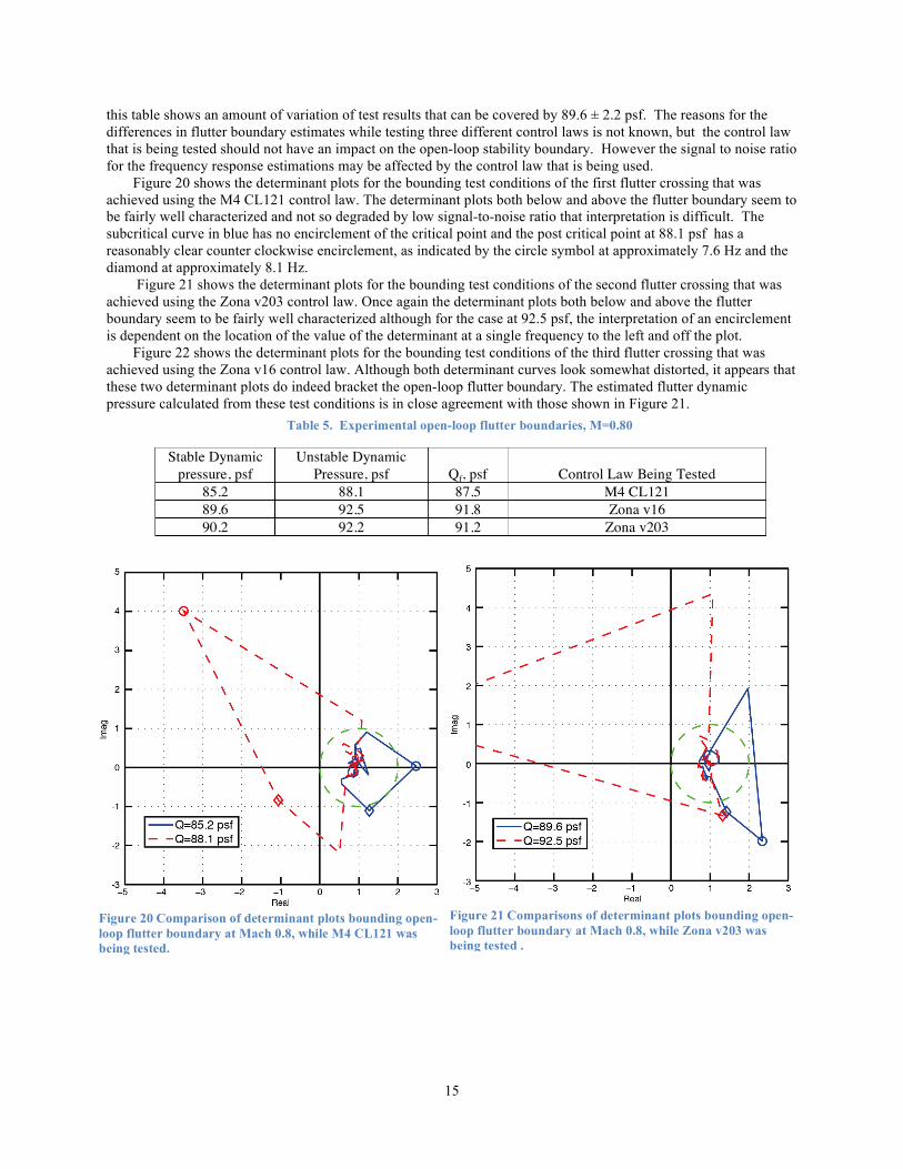
Table 5 shows the results of these calculations using the points below and above the flutter boundary of the test for Mach 0.80. At Mach 0.80, three flutter suppression control laws suppressed flutter above the open-loop flutter boundary. The table identifies the dynamic pressures below and above the open-loop flutter boundary, and the control law which was being tested at the time of each open-loop flutter crossing. The control law names were provided by the control law designers. All three Mach 0.80 control laws used the horizontal tail for control and the NIBAFTZ as the sensor. More details regarding their order and properties are provided in the reference17.

For the second and third open-loop flutter boundary crossings corresponding to the second and third rows of Table 5, the estimated flutter dynamic pressures are within the bounds of both brackets. The brackets associated with the first crossing do not even overlap the brackets associated with the second and third crossing. The resulting estimates of the flutter dynamic pressure, 87.5 psf through 91.8 psf, agree with each other within less than 5 psf so

Figure 18 Comparison of determinant plots, open and closed-loop CPE, Mach 0.80, Q 70 psf.

Figure 19 Comparison of closed loop robustness from open-loop and closed-loop CP, Mach 0.80, Q 70 psf.

15

this table shows an amount of variation of test results that can be covered by 89.6 ± 2.2 psf. The reasons for the differences in flutter boundary estimates while testing three different control laws is not known, but the control law that is being tested should not have an impact on the open-loop stability boundary. However the signal to noise ratio for the frequency response estimations may be affected by the control law that is being used.

Figure 20 shows the determinant plots for the bounding test conditions of the first flutter crossing that was achieved using the M4 CL121 control law. The determinant plots both below and above the flutter boundary seem to be fairly well characterized and not so degraded by low signal-to-noise ratio that interpretation is difficult. The subcritical curve in blue has no encirclement of the critical point and the post critical point at 88.1 psf has a reasonably clear counter clockwise encirclement, as indicated by the circle symbol at approximately 7.6 Hz and the diamond at approximately 8.1 Hz.

Figure 21 shows the determinant plots for the bounding test conditions of the second flutter crossing that was achieved using the Zona v203 control law. Once again the determinant plots both below and above the flutter boundary seem to be fairly well characterized although for the case at 92.5 psf, the interpretation of an encirclement is dependent on the location of the value of the determinant at a single frequency to the left and off the plot.

Figure 22 shows the determinant plots for the bounding test conditions of the third flutter crossing that was achieved using the Zona v16 control law. Although both determinant curves look somewhat distorted, it appears that these two determinant plots do indeed bracket the open-loop flutter boundary. The estimated flutter dynamic pressure calculated from these test conditions is in close agreement with those shown in Figure 21.

Table 5. Experimental open-loop flutter boundaries, M=0.80

Stable Dynamic pressure, psf

Unstable Dynamic Pressure, psf Qf, psf Control Law Being Tested

85.2 88.1 87.5 M4 CL121 89.6 92.5 91.8 Zona v16 90.2 92.2 91.2 Zona v203

Figure 21 Comparisons of determinant plots bounding open-loop flutter boundary at Mach 0.8, while Zona v203 was being tested .

Figure 20 Comparison of determinant plots bounding open-loop flutter boundary at Mach 0.8, while M4 CL121 was being tested.

16

The Mach 0.95 open-loop flutter boundary was traversed twice during the wind-tunnel test with the same MIMO control law, Zona v448. For the first crossing, the closed-loop CPE was conducted using multisine excitations sent simultaneously to both control surfaces, FLAP and the HT. For the second crossing, the closed-loop CPE was conducted using multisine excitations sent to the FLAP and HT one at a time.

The results are summarized in Table 6. The flutter boundary estimate from the first crossing is within both flutter boundary brackets. The second crossing estimate is outside the bracket of the first flutter crossing. The time histories were examined to ascertain whether there were any non-linearities such as hitting the limits of travel for either of the control surfaces being used. There were no such linearities found. The two estimates result in a flutter boundary estimate is 93.1 ± 1.5 psf. Figure 23 shows the determinants of the bounding test conditions for the first flutter crossing. As with figure 21 there is a fair amount of distortion apparent in these determinant plot curves. A reasonable interpretation is that the curve at 90.2 psf does not encircle the critical point but the curve at 93.0 psf does encircle the critical point, indicated a valid bracket for the open-loop flutter boundary crossing.

Figure 24 shows the determinants of the bounding test conditions for the second flutter crossing. The interpretation of the 91.3 psf curve is fairly conclusive that it is below the open-loop flutter boundary. The interpretation of the curve at 95.3 psf is somewhat more problematic. However there are 3 data points below 7.6 Hz that seem to indicate a well formed encirclement of the critical point. The actual figure is very dependent on where to the determinant values are for two frequencies. In all likelihood, this represents a condition above the open-loop flutter boundary, but the interpolation based on the reciprocal of the maximum singular values of the plant may lead to a higher flutter dynamic pressure estimate than is in fact the case. Therefore taking the determinant plots for both flutter crossings into consideration, the open-loop flutter boundary may be closer to 91.6 psf than to 94.6 psf.

The experimental flutter boundary at Mach 1.10 was not determined because the testing was limited to 101 psf for model safety reasons. Coming down in tunnel speed from a condition above 101 psf would traverse the region of open-loop instability at Mach 0.95 and it was not considered feasible to rely on a Mach 1.10 control law to traverse the region of open-loop instability at lower Mach numbers.

Comparisons of the experimental and analytical flutter boundaries are shown in Figure 25 - 26. Figure 25 compares the flutter dynamic pressures of the analytical models, shown in table 3, with the experimental flutter boundary estimates provided in tables 5 and 6. Figure 26 compares the flutter frequencies of the analytical models shown in table 4 with the experimentally derived flutter frequencies. The experimentally derived flutter frequencies were estimated by interpolating the frequencies at which the reciprocal maximum singular value of the open-loop plant occur to the open-loop flutter dynamic pressure. The experimentally derived flutter frequencies for all Mach numbers was approximately 7.7 Hz ±0 .2441 Hz which is the frequency resolution using the 4k blocksize for processing the frequency responses.

Table 6. Experimental open-loop flutter boundaries, M=0.95, Zona_v448 control law being tested

Stable Dynamic Pressure, psf

Unstable Dynamic Pressure, psf Qf, psf

Multisine Excitations Sent to Model

90.2 93.0 91.6 Simultaneous 91.3 95.3 94.6 Individual

Figure 22 Determinant plots bounding open-loop flutter boundary at Mach 0.8, while Zona v16 was being tested

17

Figure 26 Flutter frequencies for S4T Model.

VIII. Future Work

Although the S4T wind tunnel program has concluded, the MATLAB/Simulink simulation developed under the

program provides an opportunity for future research and analysis to improve the CPE methodology and gain an understanding of the uncertainties associated with the estimation of frequency responses from time histories. The impact of processing parameters, ie blocksize, windowing, overlap can be more thoroughly investigated using time histories generated from the digital simulation because they can be compared with the frequency responses calculated directly from the analytical plant models used in the simulation. The simulation provides the opportunity to investigate the signal to noise ratio impact on the frequency response calculations and the resulting CPE results. The amplitude of the turbulence can be modified to investigate signal to noise issues associated with turbulence. Different types of excitations with different frequency content and phasing can be investigated more thoroughly. The amplitude of the excitation can also be varied to assess the impact on the signal-to-noise ratio. Under the S4T

Figure 24 Determinant plots bounding open-loop flutter boundary at Mach 0.95, individual excitations to FLAPEXC and HTEXC.

Figure 25 Flutter dynamic pressures for S4T model

Figure 23 Determinant plots bounding open-loop flutter boundary at Mach 0.95, simultaneous excitations to FLAPEXC and HTEXC

18

program, reduced order models using non-linear CFD codes are being developed20. These models can be implemented in the simulation and investigated using CPE and compared with the experimental test results. The end result of this future work will be to improve the CPE procedure, reduce uncertainties associated with the calculation of the frequency responses and obtain more reliable CPE results and improved test procedures for future active controls tests in the TDT.

IX. Concluding Remarks

The S4T wind tunnel model is a sophisticated aeroelastically scaled model with multiple sensors and active

control surfaces which was tested under the Fundamental Aeronautics program. The analytical and experimental evaluation of the control law performance in terms of stability and robustness of the closed-loop system was essential to the success of the program. The open-loop flutter boundary was determined from closed loop experimental data. Future work using this experimental data set and simulation will improve the CPE tools, and will enhance future active controls work.

References

1. Perry,B., III; Silva ,Walter A.; Florance , J. R.; Wieseman, C. D.; Pototzky , A.S.; Sanetrik , M.D.; Scott, R.C.; Keller, D.F.; Cole, S.R. and Coulson, D.A.; “Plans and Status of Wind-Tunnel Testing Employing an Aeroservoelastic Semispan Model”, AIAA 2007-1770, presented at 48th AIAA SDM Conference.

2. Silva, W. A., Perry, B., Florance, J. R., Sanetrik, M. D., Wieseman, C. D., Stevens, W. L., Funk, C. J., Hur, J., Christhilf, D. M., and Coulson, D. A.., “An Overview of Preliminary Computational and Experimental Results for the Semi-Span Super-Sonic Transport (S4T) Wind-Tunnel Model," International Forum of Aeroelasticity and Structural Dynamics, Vol. IFASD-2011-147, Paris, France, 2011.

3. Silva, W.A.; Perry,B., III; Florance , J. R.; Sanetrik , M.D; Wieseman, C.D; Stevens, C.J, Hur, J. Christhilf,D.M; Coulson, D. A. “An Overview of the SemiSpan Supersonic Transport (S4T) Wind-tunnel model program”, AIAA paper submitted to 53rd SDM Conference.

4. Florance, J. R; Silva, W. A; Perry, B, III; Sanetrik M D.; Scott, R.C.; Keller, D.F; “Design, Fabrication and Characterization of the SemiSpan Supersonic Transport (S4T) Wind-Tunnel Model,” AIAA paper submitted to 53rd SDM Conference.

5. Christhilf, D.M., Pototzky, A.S. and Stevens, W.L.; “Incorporation of SemiSpan SuperSonic Transport (S4T) Aeroservoelastic Models into SAREC-ASV Simulation,” AIAA 2010-8099, presented at the AIAA Modeling and Simulation Technologies Conference, Ontario, Canada.

6. Wieseman, C.D., Hoadley, S.T. and McGraw, S.M., “On-line analysis capabilities developed to support the AFW Wind-tunnel tests,” Journal of Aircraft, Vol. 32, No. 1, Jan-Feb 1995.

7. Pototzky, A.S., Wieseman, C.D., Hoadley S.T. and Mukhopadyay, V.; “On-Line Performance Evaluation of Multiloop Digital Control Systems,” Journal of Guidance, Control and Dynamics, Vol. 15, No. 4, July-August 1992.

8. Durham, M.H.; Keller, D.F.; Bennett, R.M.; and Wieseman, C.D.: “A Status Report on a Model for Benchmark Active Controls Testing.” AIAA Paper No. 91-1011.

9. Waszak, M.R.: “Modeling the Benchmark Active Control Technology Wind-Tunnel Model for Application to Flutter Suppression.” AIAA Paper No. 96-3437. Presented at the AIAA Atmospheric Flight Mechanics Conference. San Diego, CA. July 29-31, 1996

10. McGowan, A.-M. R., Heeg, J., Lake, R.C, “Results of wind-tunnel testing from the piezoelectric aerostatic response tailoring investigation” AIAA-1996-1511 AIAA/ASME/ASCE/AHS/ASC Structures, Structural Dynamics, and Materials Conference and Exhibit, 37th, Salt Lake City, UT, Apr. 15-17, 1996, Technical Papers. Pt. 3 (A96-26801 06-39)

11. Moses, R. W., “Vertical Tail Buffeting Alleviation Using Piezoelectric Actuators - Some Results of the Actively Controlled Response of Buffet- Affected Tails (ACROBAT) Program,” SPIE’s 41h Annual International Symposium on Smart Structures and Materials, San Diego, CA, 4-6 March 1997.

12. Roughen, K. M. and Bendiksen , O.O.; “Active Flutter Suppression of the Supersonic Semispan Transport (S4T) Model,” AIAA Paper 2010-2621, presented at the 51st AIAA SDM Conference, Orlando, FL.

13. Roughen, K.M., Bendiksen, O.O and Gadient, R.; “Active Aeroelastic Control of the Supersonic Semispan Transport (S4T) Model”; AIAA Paper 2010-8397, presented at AIAA Guidance Navigation and Control Conference, Ontario, Canada.

19

14. Chen, P.C., B.; Moulin, B.; Ritz, E.; Lee, D.H.; and Zhang, Z. “CFD-based Aeroservoelastic Control for Supersonic Flutter Suppression, Gust Load Alleviation and Ride Quality Enhancement,” AIAA Paper 2009-2537 presented at the 50st AIAA SDM Conference, Palm Springs, CA.

15. Moulin, B.; Ritz, E.; Chen, P.C.; Lee, D.H.; and Zhang, Z. “CFD-based Control for Flutter Suppression, Gust Load Alleviation and Ride Quality Enhancement for the S4T Model,” AIAA Paper 2010-2623 presented at the 51st AIAA SDM Conference, Orlando, FL.

16. Moulin, B.; Ritz, E.; Florance, J.R.; Sanetrik, M.D.; and Silva, W.A.; “CFD-based Classic and Robust Aeroservoelastic Control for the SuperSonic SemiSpan Transport Wind-Tunnel Model,” AIAA Paper 2010-7802 presented at the AIAA Atmospheric Flight Mechanics Conference, Ontario, Canada.

17. Christhilf, D.M. , Moulin, B., Ritz E., Chen P. C, Roughen, K.M, ; Perry III, Boyd; “Characteristics of Control Laws Tested on the Semi-Span Super-Sonic Transport (S4T) Wind-Tunnel Model,” AIAA paper submitted to 53rd SDM Conference.

18. Heeg, J. ; “Evaluation of Simultaneous Multisine Excitation of the Joined Wing Aeroelastic Wind Tunnel Model,” AIAA-2011-1959, presented at the 52nd AIAA/ASME/ASCE/AHS/ASC Structures, Structural Dynamics and Materials Conference.

19. Heeg, J.and Wieseman, C.D., “System identification and uncertainty quantification using orthogonal excitations and the Semispan SuperSonic Transport (S4T) model”, AIAA paper submitted to 53rd SDM Conference.

20. Sanetrik M D.; Silva, W.A., and Hur, J.; “Computational Aeroelastic Analysis of the Semi-Span Super-Sonic Transport (S4T) Wind-tunnel Model”, AIAA paper submitted to 53rd SDM Conference.