ANALYTICAL AND NUMERICAL RESULTS ON ESCAPE

OF BROWNIAN PARTICLES

by

Carey Caginalp

Submitted to the Graduate Faculty of

the Department of Mathematics in partial fulfillment

of the requirements for the degree of

Bachelor of Philosophy

University of Pittsburgh

2011

UNIVERSITY OF PITTSBURGH

DEPARTMENT OF MATHEMATICS

This dissertation was presented

by

Carey Caginalp

It was defended on

January 28, 2011

and approved by

Xinfu Chen, Mathematics Department, University of Pittsburgh

Huiqiang Jiang, Mathematics Department, University of Pittsburgh

Dehua Wang, Mathematics Department, University of Pittsburgh

Marshall Slemrod, Mathematics Department, University of Wisconsin

Dissertation Director: Xinfu Chen, Mathematics Department, University of Pittsburgh

ii

Copyright c by Carey Caginalp

2011

iii

 

ANALYTICAL AND NUMERICAL RESULTS ON ESCAPE

OF BROWNIAN PARTICLES

Carey Caginalp, B-Phil

University of Pittsburgh

Abstract. A particle moves with Brownian motion in a unit disc with reflection from the

boundaries except for a portion (called "window" or "gate") in which it is absorbed. The main

problems are to determine the first hitting time and spatial distribution. A closed formula for the

mean first hitting time is given for a gate of any size. Also given is the probability density of the

location where a particle hits if initially the particle is at the center or uniformly distributed.

Numerical simulations of the stochastic process with finite step size and sufficient amount of

sample paths are compared with the exact solution to the Brownian motion (the limit of zero step

size), providing an empirical formula for the divergence. Histograms of first hitting times are

also generated.

iv  

TABLE OF CONTENTS

1.0 INTRODUCTION . . . . . . . . . . . . . . . . . . . . . . . . . . . . . . . . . 1

2.0 MAIN RESULTS . . . . . . . . . . . . . . . . . . . . . . . . . . . . . . . . . . 6

3.0 PROOF OF THE MAIN RESULTS . . . . . . . . . . . . . . . . . . . . . . 8

4.0 MONTE�CARLO SIMULATIONS . . . . . . . . . . . . . . . . . . . . . . 15

BIBLIOGRAPHY . . . . . . . . . . . . . . . . . . . . . . . . . . . . . . . . . . . . 20

v

LIST OF FIGURES

1 Movement of a particle subject to Brownian motion. . . . . . . . . . . . . . . 4

2 Histograms for the escape times of 400,000 sample paths for various gate and

step sizes. . . . . . . . . . . . . . . . . . . . . . . . . . . . . . . . . . . . . . . 16

3 Relative and absolute error for various gate and step sizes. . . . . . . . . . . . 18

4 Representation of relative and absolute error for various gate and step sizes

using a three-dimensional plot. . . . . . . . . . . . . . . . . . . . . . . . . . . 18

5 Cdf (cumulative distribution function) and ecdf (empirical cumulative distrib-

ution function) of the exit position along the gate. . . . . . . . . . . . . . . . 19

vi

1.0 INTRODUCTION

Many physical, chemical, biological, and ecological processes can be formulated in terms of

a Brownian motion with re�ection at most of the domain boundary and absorption from a

small part. In chemical processes [10], particle A may move around randomly while B is

essentially stationary, and a reaction occurs when A enters an attraction basin of B. In cell

biology, an ion drifts about within a cell, is re�ected when it hits the membrane, which is

most of the boundary of the cell, and escapes when it hits a small pore, thereby altering

the electrostatic balance in and out of the cell [4]. A prey moving randomly in a con�ned

territory dies when it encounters a predator hiding at the entrance to the territory [7]. An

epidemic con�ned in one region may spread through small unsecured boundary of the region.

These applications thus lead to a pure mathematical problem of �nding the expected life

time (mean �rst passage time or MFPT) of a Brownian particle (or a particle subject to

Browian motion) in an n-dimensional domain in which the particle is re�ected from @n�

and dies (or escapes or is absorbed) once it hits � � @. We de�ne a Brownian Motion as

a real-valued stochastic process w (t; !) on R+ � that satis�es the following properties:

(1) w (0; !) = 0 with probability 1.

(2) w (t; !) is a continuous function of t almost everywhere.

(3) For every t; s � 0; the increment �w (s) = w (t+ s; !) � w (t; !) is independent of

events prior to t, and is a zero mean Gaussian random variable with variance

V ariance := E j�w (s)j2 = s:

This problem has been studied by several authors ([2, 3, 5, 6, 7, 9] and references therein).

Most recently, Chen and Friedman [1] proved asymptotic expansions for MFPT when the

size of the gate, �, is small.

1

In this paper, we start with the equation

d�!x = �!b dt+ �d�!w ((1.1))

where ~w = [w1 (t) ; :::; wn (t)]T is Brownian motion in n dimensions. Here � is the n � n

covariance matrix, whose entries determine the changes in the x1; :::; xn directions based on

a speci�cation of the noise d~w. For example, if � = In�n; then the change in xi depends

only on the change in wi. ~x is the position of the particle, so that d~x is the change in the

particle�s position, and ~b is the drift velocity. We will assume that the drift velocity is zero

and that the covariance matrix is the identity I, so that the motion of the particle along

Later, this will be approximated in the numerics by ~x (t+�t) = ~x (t) + !� ~N (0; 1)�t. We

present a closed formula for MFPT for the fundamental case when is the unit disc and �

is a connected arc on the boundary.

From an analytical point of view this formula provides the exact size of O(1) in several

asymptotic expansions derived in the past [1, 2, 4, 5, 9]. Singer, Schuss, and Holcman [9]

obtained an approximation for the mean escape time up to an O (1) term from the center of

a disc E :

T (z) =jjD�

�log

�1

"

�+O (1)

�; z 2 E:

where jj is the area contained in . For the case of the unit disc (denoted by B), D = 4

and jj = �. Recently, Chen and Friedman [1] obtained the approximation

T (z) =1� jzj2

4�+1

�ln

�2 j1� zj"

�+O (") +

O ("2)

dist (z;�")2 for z 2 B

for the mean escape time, and by using the mean value theorem for harmonic functions, they

obtain the average mean escape time

�T =1

8�+1

�ln

�2

"

�+O (") ;

both of which are accurate up to an O (") term. Using rigorous asymptotic analysis, they

show that these estimates are accurate under the condition dist(z;�") < 3" (i.e., the particle

does not start too close to the gate). We call the case fundamental since upon which asymp-

totic expansions for general domains with multiple small windows can be derived [1]. From

a numerical point of view, this formula provides a reliable test for any numerical algorithm

2

designed to tackle the case when the gate size is very small (so the numerical problem is very

sti¤). In general without knowing the exact size of O(1)j�j or even O(1)j�j2 where j�j is the

length of �, an asymptotic expansion is quite often very hard to verify or use, since one cannot

easily determine whether the di¤erence between the numerical solution and the asymptotic

expansion is due to the error of discretization or due to the error, say, O(1)j�j log j�j, of the

underlying asymptotic expansion. Our closed formula provides a concrete criterion here.

As a consequence of the relationship between the stochastic problem and elliptic equa-

tions (see Theorem 1) one can compute numerical solutions on MFPT using Poisson�s equa-

tion. Here we shall use a Monte�Carlo method directly simulating the di¤usion process

and computing related statistics. A simple Monte-Carlo simulation can produce tremendous

amount of useful information. For example, from a reasonable amount (> 20) of sample

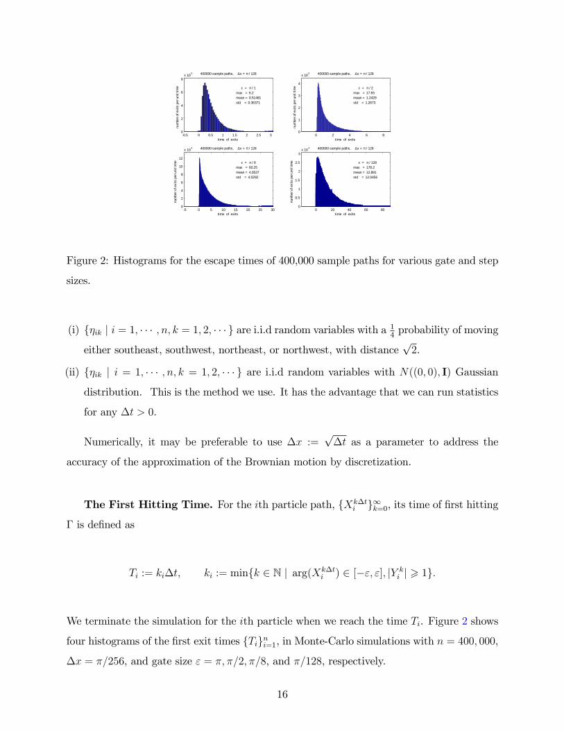
paths, we can construct a histogram of exit times (c.f. Figure 2) from which we can compute

the mean (i.e. MPFT), the variance, the probability density (and its exponential tail), etc.,

of the �rst passage times; also from the locations of exits, we can construct histograms as

well as empirical cumulative distribution functions (c.f Figure 5) to �nd where the particle

exits. A single 2GHz processor can produce 106 sample paths per hour, if the time step, �t,

and size of the gate are not too small, say �t > 10�5 and j�j > 10�1. In applications, thiswill be su¢ cient to provide needed information for actions of optimal controls.

Our Monte-Carlo simulation is based on the following stochastic process fXt; Ytgt2Tde�ned by

Yt+�t = Xt +p�t �t; Xt+�t =

Yt+�tmaxf1; jYt+�tj2g

8 t 2 T :=1[k=0

fk�tg; (1.1)

where X0 = Y0 are given and f�tgt2T are i.i.d random variables with (normal) N(0; I)

distribution. The �rst passage time associated with the process is de�ned by

� � = minnt 2 T

��� Ytmaxf1; jYtjg

2 �o: (1.2)

In simulation, �rst of all, there is a random error due to the statistical sampling. Trusting the

quality of common random number (CRN) generator that we use, this error can be controlled

by taking an appropriate large number of samples, as a consequence of the Central Limit

Theorem. There is also a discretization error due to the approximation of (1.1) to the

3

Figure 1: Movement of a particle subject to Brownian motion.

4

di¤usion process, fWtgt>0, of the Brownian motion con�ned in the unit disc with pure

re�ection on the boundary. With an exact solution for the particular case of the circle, one

can then obtain empirical results as step size and gate size vary. Thus, a careful comparison

of the exact solution with the numerical solution illuminates the distinction between �nite

step and continuous di¤usion.

We would like to point out that replacing the N(0; I) distribution of �t by a certain

transition distribution that depends on Xt will diminish the discretization error. We hope

that one can either �nd a convenient way to use the transition density from Wt to Wt+�t

to eliminate the discretization error or �nd the asymptotic behavior, as �t ! 0, of the

distribution di¤erence between fXtgt2T and fWtgt>0 and also the distribution di¤erence

between the stopping time � � de�ned in (1.2) and the �rst passage time � := infft > 0 j Wt 2

�g to produce a correction for the discretization error. Our simulation withX0 = (0; 0) = W0

suggests that

1

2� 2 log

�sinj�j4

�= E[� ] � E[� �]� 4

p�t

j�j ; std[� �] � E[� �];

where E stands for expectation and std the standard deviation; see Figures 2 and 4 where

" = j�j=2, �x =p�t, and MCT is the sample mean � E[� �] + N(0; std[� �]2=n) with

n = 400; 000.

The rest of the paper is organized as follows. We present our theoretical results for E[� ]

and std[� ] in Section 2, their proofs in Section 3, and results of Monte-Carlo simulations in

Section 4.

5

2.0 MAIN RESULTS

Our starting point is the formulation for the statistics of the stochastic process as solutions

of di¤erential equations. The following equation for the mean �rst passage time is a standard

result [8], while the expression for its variance is new.

Theorem 1. Let be a bounded domain with smooth boundary @ and � be a closed subset

of @. For each x 2 , let �x be the �rst time of a particle hitting �, assuming that the

particle starts from x, is subject to the Brownian motion in , and re�ects from @. Then,

the mean �rst passage time, T (x) := E[�x], and its variance, v(x) := E[(�x � T (x))2], are

solutions of the following boundary value problems:

��T = 2 in ; T = 0 on �; @nT = 0 on @ n �; (2.1)

��v = 2jrT j2 in ; v = 0 on �; @nv = 0 on @ n �: (2.2)

Here @n := n � r is the derivative in the direction n, the exterior normal to @:

Moreover, the average of the variance can be calculated from the formula

�v :=1

jj

Z

v(x)dx =1

jj

Z

T 2(x)dx =: T 2: (2.3)

The main contribution of this paper is the following closed formula for the mean �rst

passage time in a special case that has attracted much attention and been the subject of

many theoretical investigations in the past; see [1, 2, 5, 9] and the references therein.

6

Theorem 2. (A Closed Formula) In 2-D, with points identi�ed by complex numbers, let

:= frei� j 0 6 r < 1;�" 6 � 6 2� � "g; � := fei� j j�j 6 "g: (2.4)

Then the mean �rst passage time T (z), for z 2 �, is given by

T (z) =1� jzj22

+ 2 log

�����1� z +p(1� ze�i")(1� zei")2 sin "

2

����� : (2.5)

For the rest of this paper, we will assume and � are as in (2.4). This exact formula

allows us to improve the result of Theorem 5.1 in [1] by the following.

Theorem 3. The mean �rst passage time T has the following properties:

T (0) =1

2� 2 log

�sin"

2

�; �T :=

1

jj

Z

T (x)dx = T (0)� 14;

T (ei�) = 2 arccoshmaxfsin "

2; j sin �

2jg

sin "2

8 � 2 R:

In addition, setting "̂ = 2 sin "2= jei" � 1j, we have, when 0 < "̂ 6 j1� zj and z 2 �,

T (z) =1� jzj22

+ 2 log2j1� zj"̂

+ <�

z"̂2

2(1� z)2

�+O(1)z2"̂4

j1� zj4

where < stands for the real part and O(1) is a certain function satisfying jO(1)j < 0:887 :

Finally we consider the location of a particle when it exits.

Theorem 4. The probability density of the location of a particle at time of its exit is given

by

�j(ei�) := � 12�

@

@rT (ei�) =

8>><>>:0 if " < � < 2� � ";1

2�

cos �2q

sin2 "2� sin2 �

2

if j�j < ":

That is, for any (Borel set) � @, the probability that a particle, starting either at the

origin or uniformly distributed in , making Brownian motion in , re�ecting when it hits

@ n �, and escaping once it hits �, ends up escaping from is

P ( ) =

Z

�j(y)dSy

where dSy is the surface element of @ at y 2 @.

These Theorems will be proven in the next section.

7

3.0 PROOF OF THE MAIN RESULTS

Proof of Theorem 1. For convenience, we call a particle dead as soon as it hits �; otherwise

survived. For x 2 , we denote by �(x; �; t) the survival probability density at time t of the

particle starting from x; that is, �(x; y; t)dy is the probability that a particle starting from

x lands in the region y + dy at time t before it hits �. Then by the Kolmogrov equation,

8>>>>>>>>>><>>>>>>>>>>:

�t =12�� in � (0;1);

� = 0 on �� (0;1);

@n� = 0 on (@ n �)� (0;1);

�(x; �; 0) = �(x� �) on � f0g

(3.1)

where �(x��) is the Dirac mass concentrated at x. If we denote by � the principal eigenvalue

of the operator �12� subject to the mixed Neumann(zero on @ n �)�Dirichlet(zero on �)

boundary condition, then

0 6 �(x; y; t) 6 Ce��t 8 y 2 �; t > 1; x 2

where C is some positive constant. Since � is positive, we see that � decays in time expo-

nentially fast.

Next we introduce the function

G(x; y) :=1

2

Z 1

0

�(x; y; t)dt 8x 2 ; y 2 �:

8

Then it is easy to see that G(x; �) = 0 on � and @nG(x; �) = 0 on @ n �. In addition

��G(x; �) = �12

Z 1

0

��(x; �; t)dt = �Z 1

0

�t(x; �; t)dt = �(x; �; 0) = �(x� �):

Thus, G is indeed the Green�s function of the Laplace operator � associated with the

Neumann-Dirichlet boundary condition; that is, for every x 2 , G(x; �) is the solution

of

��G(x; �) = �(x� �) in ; G(x; �) = 0 on �; @nG(x; �) = 0 on @ n �:

Note that the probability that a particle starting from x survives at time t is

p(x; t) :=

Z

�(x; y; t)dy:

Consequently, the probability that a particle dies in the time interval [t; t + dt) is p(x; t) �

p(x; t+ dt). Hence, the expected life time (mean �rst passage time) is given by

T (x) := E[�x] =Z 1

0

tnp(x; t)� p(x; t+ dt)

o= �

Z 1

0

tpt(x; t) dt

=

Z 1

0

p(x; t)dt =

Z 1

0

Z

�(x; y; t)dydt =

Z

2G(x; y)dy

where we have used integration by parts in the third equation. Since G is the Green�s

function, T is therefore the solution of the mixed Neumann-Dirichlet boundary value problem

(2.1).

In Monte�Carlo simulations, con�dence intervals are estimated in terms of the standard

deviation, �(x), of the exit time �x, de�ned by

�(x) =pv(x); v(x) = E[(�x � T (x))2] = E[� 2x ]� T (x)2:

To calculate v, we introduce

�1(x; y; t) =

Z 1

t

�(x; y; s)ds:

9

Then for �xed x 2 and t > 0, �1(x; �; t) satis�es

�1(x; �; t) = 0 on �; @n�1(x; �; t) = 0 on n �; �1(x; �; 0) = 2G(x; �) on :

Also,

1

2��1(x; �; t) =

Z 1

t

1

2��(x; �; s)ds =

Z 1

t

�s(x; �; s) ds = ��(x; �; t) = �1t(x; �; t) in :

Thus,

E[� 2x ] =Z 1

0

t2np(x; t)� p(x; t+ dt)

o= �

Z 1

0

t2pt(x; t)dt =

Z 1

0

2tp(x; t)dt

=

Z 1

0

2t

Z

�(x; y; t)dydt = �2Z

Z 1

0

t�1t(x; y; t)dtdy

= 2

Z

Z 1

0

�1(x; y; t)dtdy = �Z 1

0

Z

�1(x; y; t)�T (y)dydt

= �Z 1

0

Z

T (y)�y�1(x; y; t)dydt = �2Z

Z 1

0

T (y)�1t(x; y; t)dtdy

= 2

Z

T (y)�1(x; y; 0)dy =

Z

4T (y)G(x; y)dy:

This means that M(x) := E[� 2x ] satis�es

��M = 4T in ; M = 0 on �; @nM = 0 on @ n �:

Consequently, v =M � T 2 is the solution of (2.2).

Finally, we prove (2.3) as follows:

�v :=1

jj

Z

v(x)dx = � 1

2jj

Z

v(x)�T (x)dx = � 1

2jj

Z

T (x)�v(x)dx

=1

jj

Z

T (x)jrT (x)j2dx = 1

2jj

Z

rT 2(x) � rT (x)dx

= � 1

2jj

Z

T 2(x)�T (x)dx =1

jj

Z

T 2(x)ds:

This completes the proof of Theorem 1.

10

Remark 5. The transition probability density from Wt = x to Wt+�t = y for the di¤usion

process of Brownian motion con�ned in with re�ection boundary n � and absorption

boundary � is �(x; y;�t) where � is the solution of (3.1). Thus, the exact discretization of

the di¤usion process is

Wt+�t = Wt + �k(Wt) 8 t 2 T := [1k=0fk�tg

where f�kg1k=0 are independent random variables and �k(x) has probability density �(x; �;�t).

Our Monte-Carlo process de�ned in (1.1) with �t � N(0; I) is just a convenient approxima-

tion for t 2 [0; � ] \T.

Proof of Theorem 2. We need only show that T given in (2.5) satis�es (2.1). For this,

we use <(z) and =(z) to denote the real and imaginary part of a complex number z. Notice

that in default, for z 2 we have

<�1� z +

p(1� ze�i")(1� zei")

�= <(1� z) + <

p(1� ze�i")(1� zei") > 0:

Hence, taking a real value at z = 0, the function

f(z) := 2 log1� z +

p(1� ze�i")(1� zei")2 sin "

2

is analytic in � n fei"; e�i"g and continuous on �. Consequently, its real part, <(f), is

harmonic in . Hence,

�T (z) = �1� jzj22

+ �<(f(z)) = �1� jzj2

2= �2 8 z 2 :

Next, for z 2 �, we can write z = ei� with j�j 6 ". Then

f(ei�) := limr%1

2 log1� rei� +

p(1� rei[��"])(1� rei[�+"])2 sin "

2

= 2 loghei�=2

qsin2 "

2� sin2 �

2� i sin �

2

sin "2

i= i�� � 2 arcsin

sin �2

sin "2

�8 � 2 [�"; "]:

Thus, <(f(z)) = 0 when z 2 �. Consequently, T (z) = 0 on �.

11

Similarly, for z 2 @ n �, we write z = ei� with � 2 ("; 2� � ") to obtain

limr%1

argq(1� rei[��"]))(1� rei[�+"]) = 1

2

�� �2+� � "2

�� 12

��2� "+ �

2

�=� � �2:

Hence,

f(ei�) := limr%1

f(rei�) = 2 loghei(���)=2

sin �2+qsin2 �

2� sin2 "

2

sin "2

i= (� � �)i+ 2 arccosh

sin �2

sin "2

8 � 2 ["; 2� � "]:

Here arccosh : [1;1)! [0;1) is de�ned by arccosh z := log[z +pz2 � 1] for z > 1. It then

follows from the Cauchy-Riemann equation that in the polar coordinates (r; �),

@

@r<(f(ei�)) = @

@�=(f(ei�)) = 1 8 � 2 ("; 2� � "): (3.2)

Hence, for z 2 @ n �,

@nT (z) =@

@r

1� jzj22

+@

@r<(f(z)) = 0:

Therefore, by the uniqueness of the solution of problem (2.1), T is given by the formula

(2.5). This completes the proof of Theorem 2.

Proof of Theorem 3. The formula T (0) and T (ei�) follows directly from (2.5) and the

calculation of f(ei�) in the proof of Theorem 2. Also, by the Mean Value Theorem for

harmonic functions,

�T =1

jj

Z

(1� jxj2)2

dx+ <f(0) = 1

4+ 2 log

1

sin "2

= T (0)� 14:

For the asymptotic (indeed Taylor) expansion, we can write T in (2.5) as

T (z) =1� jzj22

+ 2 logj1� zjsin "

2

+ 2< log 1 +p1 + b2

2; b :=

2pz sin "

2

1� z =

pz"̂

1� z :

When 0 < "̂ 6 j1� zj and z 2 �, we have jbj < 1. Applying the maximum principle for the

analytic �nction ��2flog 1+p1+�2� �

4g on the unit disc we �nd that��� log 1 +p1 + �

2� �4

��� 6 � ln 2� 14

�j�j2 6 0:4432j�j2 8 j�j 6 1:

The stated expansion for T thus follows.

12

Remark 6. (1). It is clear from (2.5) that the function T is smooth (C1) in � n fei�; e�i�g

and Hölder continuous with exponent 12on �.

(2). The constant �T is the average of the mean exit time. It was derived in [4, 9] in the

case of one absorbing window, and in [5] for the case of a cluster of small absorbing windows

that

�T = 2 log2

"+O(1):

In [1, Theorem 5.1], it was rigorously shown that

�T =1

4� 2 log

�sin"

2

�+O(1)":

Clearly, our formula shows that the above O(1) term is indeed exactly zero.

Proof of Theorem 4. The �ux �j is calculated by using

@

@rT (ei�) = �1 + @

@�=(f(ei�))

and the expression of f(ei�).

Note that for x 2 , the quantity �12n(y) � ry�(x; y; t)dSydt is the probability that a

particle starting from x ends up escaping from dSy in time interval [t; t + dt). Hence, the

probability that a particle starting from x ends up escaping from dSy is j(x; y)dSy where

j(x; y) = �12

Z 1

0

n(y) � ry�(x; y; t)dt = �n(y) � ryG(x; y):

(1) First we consider the case that initially the particle is at x = 0. Then direct compu-

tation show that

G(0; z) = � 12�log jzj+ jzj

2 � 14�

+T (z)

2�:

Consequently,

j(0; ei�) = � @@rG(0; rei�)jr=1 = �

1

2�

@

@rT (ei�) = �j(ei�):

Thus, �j is the escaping probability density of particles starting from the origin.

13

(2) Next assume that the initial position of a particle is uniformly distributed in . Then

the probability that the particle exits from dSy is

1

jj

Z

�j(x; y)dSy

�dx

= �dSyjj

Z

�n(y) � ryG(x; y)

�dx

= �dSyjj n(y) � ryZ

G(y; x)dx = � dSy2jjn(y) � ryT (y) =

�j(y)dSy 8 y 2 @:

Thus, �j is also the escaping probability density of particles initially uniformly distributed in

. This completes the proof.

14

4.0 MONTE�CARLO SIMULATIONS

The Dicretization. We simulate the con�ned Brownian motion by n sample paths,

P1; � � � ; Pn. The sample path Pi is described by fXk�ti g1k=0 where Xk�t

i represents the posi-

tion of the particle at time t = k�t. Here fXk�ti g are random variables sequentially de�ned

by

X0i = �i0; Y ki := X

(k�1)�ti + �ik

p�t; Xk�t

i =Y ki

maxf1; jY ki j2g;

i = 1; � � � ; n; k = 1; 2; � � �

where f�10; � � � ; �n0g are the starting positions related to the initial distribution of the par-

ticle, and f�ikji = 1; � � � ; n; k = 1; 2; � � � g are i.i.d random variables with mean vector (0; 0)

and covariance matrix equal to identity. Note that Y ki is the position at time k�t of the

discretized Brownian particle if it were not bouncing from @. In our computations, we rep-

resent bouncing from the boundary @ by the Kelvin transformation z �! z=jzj2 for jzj > 1.

Other re�ection principles can also be used; for example, one can return the particle to its

position before it took the �nal step causing re�ection, or re�ect the particle geometrically

from the boundary without signi�cant change in the results provided the step size is small.

If we are simulating particles starting from a �xed point z 2 , we simply take �i0 = z for

i = 1; :::n. In the computations below we take all particles starting from the center, z = 0.

For exit times from random points, one can generate random starting points from common

random numbers (CRNs).

As long as f�ikg are i.i.d random variables with mean vector (0; 0), covariance matrix

I and �nite fourth order momentum, the limit, as �t & 0, of the piecewise linear curve

connected by points f(k�t;Xk�ti )g1k=0 is a Brownian motion path. There are two standard

choices of the i.i.d random variables f�ikg:

15

­0.5 0 0.5 1 1.5 2 2.5 30

2

4

6

8x 10 5

ε  = π / 1max   =  6.2mean =  0.51481std    =  0.36371

400000 sample paths, ∆x = π / 128

time  of  exits

num

ber o

f exi

ts p

er u

nit t

ime

0 2 4 6 80

1

2

3

4

x 10 5

ε  = π / 2max   =  17.65mean =  1.2429std    =  1.2673

400000 sample paths, ∆x = π / 128

time  of  exits

num

ber o

f exi

ts p

er u

nit t

ime

­5 0 5 10 15 20 25 300

2

4

6

8

10

12

x 10 4

ε  = π / 8max   =  60.25mean =  4.0537std    =  4.0292

400000 sample paths, ∆x = π / 128

time  of  exits

num

ber o

f exi

ts p

er u

nit t

ime

0 20 40 60 800

0.5

1

1.5

2

2.5

3x 10 4

ε  = π / 128max   =  178.2mean =  12.891std    =  12.0456

400000 sample paths, ∆x = π / 128

time  of  exits

num

ber o

f exi

ts p

er u

nit t

ime

Figure 2: Histograms for the escape times of 400,000 sample paths for various gate and step

sizes.

(i) f�ik j i = 1; � � � ; n; k = 1; 2; � � � g are i.i.d random variables with a 14probability of moving

either southeast, southwest, northeast, or northwest, with distancep2.

(ii) f�ik j i = 1; � � � ; n; k = 1; 2; � � � g are i.i.d random variables with N((0; 0); I) Gaussian

distribution. This is the method we use. It has the advantage that we can run statistics

for any �t > 0.

Numerically, it may be preferable to use �x :=p�t as a parameter to address the

accuracy of the approximation of the Brownian motion by discretization.

The First Hitting Time. For the ith particle path, fXk�ti g1k=0, its time of �rst hitting

� is de�ned as

Ti := ki�t; ki := minfk 2 N j arg(Xk�ti ) 2 [�"; "]; jY ki j > 1g:

We terminate the simulation for the ith particle when we reach the time Ti. Figure 2 shows

four histograms of the �rst exit times fTigni=1, in Monte-Carlo simulations with n = 400; 000,

�x = �=256, and gate size " = �; �=2; �=8, and �=128, respectively.

16

The Randomness Error. In a given Monte-Carlo simulation, f�ikg are generated from

CRNs according the needed distribution. The sample mean and sample standard deviation

are calculated by

T̂ =1

n

nXi=1

Ti; �̂ =

(1

n� 1

nXi=1

(Ti � T̂ )2)1=2

:

Denote by T�t = limn!1 T̂ . Then by the Central Limit Theorem, for n > 10, we can

present our conclusion from a Monte-Carlo simulation as T̂ � T�t +N(0; �̂2=n), or simply

T�t = T̂ ��̂pn

with 65% con�dence; T�t = T̂ �3�̂pn

with 99% con�dence.

In our simulations, we take n = 400; 000 particles, so the Central Limit Theorem can be

reasonably applied (recalling from the proof of Theorem 1 that the probability distribution

density of �x has an exponential tail). Our simulation (starting from (0; 0)) shows that �̂ is

proportional to T̂ with proportional constant almost equal to 1 (cf. Figure 2).

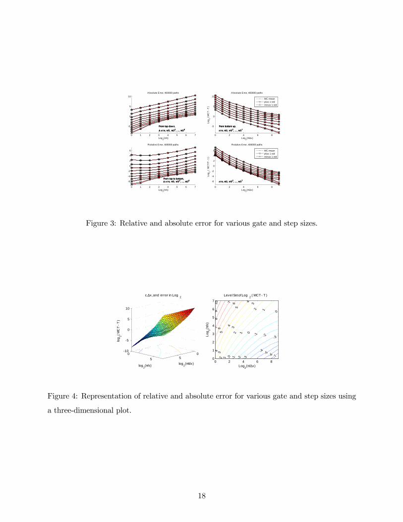
Discretization Error. Using the approximation T�t � T̂ � �̂=pn, we display the

absolute error T�t � T (> 0) and relative error T�t=T � 1 in Figures 3 and 4. From the

Figures, one sees that log2(T�t � T ) is almost linear in log2 " and in log2�x. This suggests

that

T�t � T �2�x

";

T�tT� 1 � 4�x

"(1 + 4j ln sin "2j) :

Distribution of Exits. Using the positions of the sample exits fXTii gni=1 � �, we can

�nd the sample distribution of the exits along the gate and compare it with the theoretical

density �j(y); y 2 � from Theorem 4. For �xed ", we compare the empirical cumulative

distribution function

ecdf(�) :=1

n

Xarg(X

Tii )2[�";�]

1

for various di¤erent �x, with the true

cdf(�) = P�arg(W� ) 2 (�"; �)

�=

Z �

�"�j(s)ds =

1

2+1

�arcsin

sin �2

sin "2

8 � 2 [�"; "];

17

0 1 2 3 4 5 6 7

­5

0

5

10

Log2(π/ε)

A bsolute E rror, 400000 paths

From top down,

∆ x=π, π/2, π/22, ..., π/29From top down,

∆ x=π, π/2, π/22, ..., π/29From top down,

∆ x=π, π/2, π/22, ..., π/29

0 2 4 6 8

­5

0

5

10

Log2(π/∆x)

Log 2 ( 

MC

T ­ T

 )

A bsolute E rror, 400000 paths

From bottom up,

ε=π, π/2, π/22, ..., π/27From bottom up,

ε=π, π/2, π/22, ..., π/27From bottom up,

ε=π, π/2, π/22, ..., π/27

0 1 2 3 4 5 6 7

­6

­4

­2

0

2

4

6

Log2(π/ε)

Relative E rror, 400000 paths

From top to bottom,∆ x=π, π/2, π/22, ..., π/29From top to bottom,∆ x=π, π/2, π/22, ..., π/29From top to bottom,∆ x=π, π/2, π/22, ..., π/29

0 2 4 6 8

­6

­4

­2

0

2

4

6

Log2(π/∆x)

Log 2 ( 

 MC

T/T 

­ 1 )

Relative E rror, 400000 paths

ε=π, π/2, π/22, ..., π/27ε=π, π/2, π/22, ..., π/27ε=π, π/2, π/22, ..., π/27

MC­meanplus 1 stdminus 1 std

MC­meanplus 1 stdminus 1 std

Figure 3: Relative and absolute error for various gate and step sizes.

05

05

­10

­5

0

5

10

log2(π/dx)

ε,∆x, and  error in Log2

log2(π/ε)

log 2( M

CT 

­ T )

­7­6­5­4

­3

­3

­2

­2

­1

­1

0

0

0

1

1

1

2

2

2

3

3

34

4

4

5

5

6

6

7

78

910

Log2(π/∆x)

Log 2(π

/ε)

Level Set of Log 2 ( MCT ­ T )

0 2 4 6 80

1

2

3

4

5

6

7

Figure 4: Representation of relative and absolute error for various gate and step sizes using

a three-dimensional plot.

18

­1 ­0.5 0 0.5 10

0.1

0.2

0.3

0.4

0.5

0.6

0.7

0.8

0.9

1

When ε/∆x=256, Max Error= 0.0061

θ/ε (scaled exit position e iθ)

cum

ulat

ive 

dist

ribut

ion

cdf and empirical cdfs ( ε = π/2 = 1.5708 )

0 0.2 0.4 0.6 0.8 10

0.1

0.2

0.3

0.4

0.5

0.6

0.7

0.8

0.9

1

cdf of exit position

empi

rical

 cdf

∆x=π/512=0.0061359, 400000 samples

cdf∆x=π∆x=π/2∆x=π/4∆x=π/8∆x=π/16∆x=π/32∆x=π/64∆x=π/128∆x=π/256∆x=π/512

ε=πε=π/2ε=π/4ε=π/8ε=π/16ε=π/32ε=π/64ε=π/128

Figure 5: Cdf (cumulative distribution function) and ecdf (empirical cumulative distribution

function) of the exit position along the gate.

where � is the �rst hitting time of the con�ned Brownian motion fWtg that starts from

the origin and bouncing from the unit circle. For �xed �x and various " (noting that cdf

depends on "), we consider the uniformly distributed random variable cdf(arg(W� )). This is

equivalent to plot cdf� ecdf graphs. The results are shown in Figure 5.

19

BIBLIOGRAPHY

[1] Xinfu Chen & Avner Friedman, Asymptotic analysis for the narrow escape problem,preprint.

[2] A.F. Cheviakov, M.J. Ward, & R. Straube, An asymptotic analysis of the mean �rstpassage time for narrow escape problems, Part II: The sphere, to appear in SIAM Mul-tiscale Modeling and Simulation, 30 pages

[3] I.V. Grigoriev, Y.A. Makhnovskii, A.M. Berezhkovskii, & V.Y. Zitserman, Kinetics ofescape through a small hole, J. Chem. Phys. 116 (2002), 9574�9577.

[4] D. Holcman & Z. Schuss, Escape through a small opening: receptor tra¢ cking in asynaptic membrane, J. Stat. Phys., 117 (2004), 975�1014.

[5] D. Holcman & Z. Schuss, Di¤usion escape through a cluster of small absorbing windows,J. Phys. A: Math Theory, 41 (2008), 155001.

[6] S. Pillay, M.J. Ward, A. Peirce, & T. Kolokolnikov, An asymptotic analysis of the mean�rst passage time for narrow escape problems, Part I: Two dimensional domains, toappear in SIAM Multiscale Modeling and Simulation, 28 pages.

[7] S. Redner, A Guide to First Passage Time Processes, Cambridge Univ. Press,2001.

[8] Z. Schuss, Theory and Applications of Stochastic Differential Equations:An Analytical Approach, Springer. New York, 2010.

[9] A. Singer, Z. Schuss & D. Holeman, Narrow escape, Part II: the circular disk, J. Stat,Phys, 122 (2006), 465�489.

[10] Z. Zwanzig, A rate process with an entropy barrier, J. Chem. Phys. 94 (1991), 6147-6152.

20