ANALYTICAL CO~PA~SO~ OF TWO SPATIAL DATA …delab.csd.auth.gr/papers/IS94vm.pdf · tA preliminary extended abstract of this paper appears in the Proceedings of the 4th Panhellenic

Pergamon Information Systems Vol. 1994 19, No. 7, pp. 589-582,

0306-4379(94)00027-l Copyright@ 1994 Elsevier Science Ltd Printed in Great Britain. All rights reserved

0306-4379/94 87.00 + 0.00

ANALYTICAL CO~PA~SO~ OF TWO SPATIAL DATA STRU~TURES§ $

MICHAEL VASSILAKOPOULOS’ and YANNIS MANoLoPouLos2+

* Departme nt of Electrical & Computer Eng., Aristotelian University of Thessaloniki, 54006 Thessaloniki, Greece

‘Department of Informatics, Aristotelian University of Thessaloniki, 54006 Thessaloniki, Greece

(‘Received 15 October 1993; in final revised form 11 Aupst 199.j)

Abstract - Region Quadtrees and Bintrees are two structures used in GIS and spatial databases. The expected space performances of these two trees are presented and compared. Analysis is based on the general assumption that the storage requirements of internal and external nodes differ, as well as on a parametric model of binarv random images. Initiallv. formulae that exnress the averaee total storage performance of the two tiees are given: For each” ievel of the Quadtree, formulae-for the average numbers of internal, external white and external black nodes follow. Next, for each level of the Quadtree, the relationship between each node category of the two trees is presented. Based on the formulae developed, we study how the storage requirements of the two trees differ for each Quadtree level. Finally, using the above results, we reach conclusions about the storage efficiency of the most popular implementations and the inverted variations of these two trees (structures that index pictorial databases).

1. INTRODUCTION

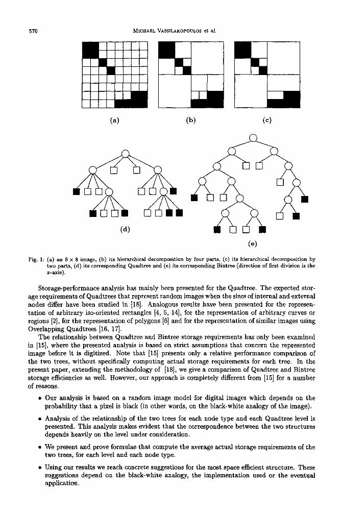
The Region Quadtree and the Region Bintree [12, 131 (called Quadtree and Bintree in the rest of this paper, for the sake of simplicity) are two popular data structures that represent digital binary images. The linear implementations of the two structures are the ones that are mainly used as basis for the physical level of Spatial Databases and Geographic Information Systems 11, 9,111. However, other implementations can serve special purposes in the same context. For example, pointer implementations can be used to structure a large main memory sequence of similar images [16] where speed of processing is essential, while Depth First (DF) expressions can support spatial database backups in stream media. Both structures are based on the principle of Hierarchical Regular Decomposition. According to this principle, if the whole image consists of pixels of the same color (white or black), then it is represented by an external node of this color. Otherwise, it is decomposed into subimages and it is represented by an internal (gray) node having as children the subtrees that correspond to these subimages. The decomposition is repeated recursively for the subtrees until the subimages created are homogenous. In the Quadtree the image is decomposed into four equal parts. These parts emerge by dividing the image along lines parallel to the two axes. In the Bintree the image is decomposed into two equal parts. These parts emerge by dividing the image along a line parallel to one of the two axes; if further decomposition is needed for at least one of the emerging subimages, then the next division takes place along a line parallel to the other axis, and so on. Note that the hierarchical decomposition is possible in the Quadtree only if the image is a quadrangle of 2n x 2” pixels, while it is possible in the Bintree only if the image is a quadrangle of 2” x 2n pixels, or a rectangle of 2”-l x 2” or 2” x 2”-i pixels, according to the direction of the first division. The decomposition is called regular because the position of the lines along which we divide is predetermined. Thus, we do not structure our data directly, but the embedding space (Image space hierarchy). An example of an 8 x 8 image is shown in figure 1.a. The hierarchical decomposition of this image by four parts and the Quadtree that represents it are shown in figures 1.b and l.d, respectively. The hierarchical decomposition of this image by two parts (starting with the zr-axis direction) and the Bintree that represents it are shown in figures 1.c and l.e, respectively.

fj Recommended by Y. Ioannidis. tA preliminary extended abstract of this paper appears in the Proceedings of the 4th Panhellenic Informatica

Conference, Patras, Greece (December 1993), pp. 59-70. tResearch partially funded by the Institute for Systems Research (ISR), while the author was with ISR and the

Computer Science Department, University of Maryland, College Park, MD 20742, USA.

569

570 MICHAEL VASSILAKOPOULOS et al.

Fig. 1: (a) an 8 x 8 image, (b) its hierarchical decomposition by four parts, (c) its hierarchical decomposition by two parts, (d) its corresponding Quadtree and (e) its corresponding Bintree (direction of first division is the z-axis).

Stor~~pe~ormance analysis has mainly been presented for the Quadtree. The expected storage requirements of Qu~tr~s that represent random images when the sizes of internal and external nodes differ have been studied in [lS]. Analogous results have been presented for the representation of arbitrary iso-oriented rectangles (4, 5, 141, for the representation of arbitrary curves or regions [2], for the representation of polygons [S] and for the representation of similar images using Overlapping Quadtrees [16, 17).

The relationship between Quadtree and Bintree storage requirements has only been examined in [15], where the presented analysis is based on strict assumptions that concern the represented image before it is digitized. Note that [15] presents only a relative performance comparison of the two trees, without specifically computing actual storage requirements for each tree. In the present paper, extending the methodology of [18], we give a comparison of Quadtree and Bintree storage e~cienci~ as well. However, our approach is completely different from [15] for a number of reasons.

Our analysis is based on a random image model for digital images which depends on the probability that a pixel is black (in other words, on the black-white analogy of the image).

Analysis of the relationship of the two trees for each node type and each Quadtree level is presented. This analysis makes evident that the correspondence between the two structures depends heavily on the level under consideration.

We present and prove formulae that compute the average actual storage requirements of the two trees, for each level and each node type.

Using our results we reach concrete su~~tions for the most space efficient structure. These suggestions depend on the black-white analogy, the implementation used or the eventual application.

Analytical Comparison of two Spatial Data Structures 571

More specifically, in section 2 we define formally the two structures and present our probabilistic assumptions. In section 3 we derive formulae for the expected total storage requirements of each

tree, taking into account the differences of node sizes. In section 4, for each level of the Quadtree, formulae for the average numbers of internal, external white and external black nodes for each level of the Quadtree follow. In section 5, for each Quadtree level, the correspondence of Quadtree and Bintree leaves and Quadtree and Bintree internal nodes is presented. In addition, based on the formulae developed, we study how the storage requirements of the two trees differ for each Quadtree level. In section 6, using the above results, we reach conclusions about the storage efficiency of the

most popular implementations of the two trees. For a particular case, we present in graphical form the breakpoint-values of black pixel probability at which the winner-structure of space efficiency

changes, as a function of the image size. In the last section, apart from summarizing the most

important results, we discuss and conclude on the space performance of the inverted variations of the two trees. These variations are used for storing a pictorial database where (fuzzy) image

pattern searching can be applied. Moreover, we give suggestions on how the random model used in this paper and the analysis that is based on it can be extended and customized for various kinds

of images.

2. DEFINITIONS AND PROBABILISTIC ASSUMPTIONS

In order to be able to compare the two trees we consider an initial 2” x 2” image. Without loss of generality, we consider that the first separation in the Bintree is along the x-axis, since the orientation of the image does not influence our analysis. Evidently, during consecutive separations the dimensions of the emerging subimages will equal 2i x2i-1 (when the separation takes place along the x-axis) and 2i-1 x 2i-1 (when the separation takes place along the y-axis), where 0 < i < n.

The Region Quadtree can be defined formally (assuming that the mathematical notion of a

tree is well known) as follows:

Definition 1 Consider the numbers n, k,x,y E N, such that k 5 n, z, y < 2” and x, y 0; 2k. Consider also the binary array 1[0. .. 2n - 1,0 ... 2n - 11. As Qn(x, y, k) we denote the tree that represents the subarray 1[x . . . x + 2” - 1, ye + s y + 2” - l] and consists of

l one external node, called a black ( white ) node, if every element of its subarray equals 1 (0), or otherwise of

l one root node, called a gray node, and its 4 children, the trees

0 Qn(x, Y, k - 11,

o Qn(x + 2k-1, y, k - l),

o Qn(x, y + 2k-1, k - 1) and

o Qn(x + 2”-i,y + 2k-1, k - 1).

The Quadtree for 1 is the tree Qn(O,O,n).

Similarly, the Region Bintree (when the first separation is along the x-axis) can be defined formally as follows:

Definition 2 Consider the numbers n, k, x, y E N, such that k 5 n, x, y < 2n and x, y o( 2k. Consider also the binary array I[0 . . . 2n - 1,O. + -2” - 11. As Bn(x, y, k) we denote the tree that

represents the subarray I[x . . . x + 2k - 1, y. . . y + 2k - l] and consists of

l one external node, called a black ( white ) node, if every element of its subarray equals 1 (0), or otherwise of


o BL(x, y, k - 1) and

o B;(x, y + 2k-1, k - 1)


As BL(s, y, Ic) we denote the tree that represents the subarray I[a . . + 2 + 2”+i - 1, y . . . y + 2” - l] and consists of

l one external node, called a black ( white ) node, if every element of its subarray equals 1 (0),

or otherwise of


The Bintree for I is the tree B,(O,O,n).

We recall a number of properties which are easily inferred from the above definitions. There are 2c4”) different images of size 2n x 2”. A Quadtree for such an image has maximum height

n. We will call such a tree a class-n Quadtree. A node that corresponds to a single pixel is at level 0, while the root is at level n. A node at level i, where 0 5 i 5 n, represents a subarray of 2i x 2i(= 4i) pixels, while there are at most 4”-i nodes at this level. A corresponding Bintree for such an image has maximum height 2n. We will call such a tree a class-2n Bintree. Note that a class-(2n - 1) Bintree represents an image of size 2n x 2+‘. A node that corresponds to a single pixel is at level 0, while the root is at level 2n. A node at level i, where 0 5 i 5 2n, represents a subarray of 21ii21 x 2ri121 (= 2i) pixels (the integer parts are used because the dimensions of the subarray depend on the orientation of the separation), while there are at most 22n--i nodes at this

level.

The probabilistic model of our images assumes that each pixel is statistically independent of any

other pixel, as far as its color is concerned. We also assume that a pixel is black with probability p and white with probability 1 - p. In the rest of the paper we will refer to p as black probability,

to 1 -p as white probability and to an image obeying this model as a random image. These mean that in the Quadtree the block corresponding to a level-i node is black with probability pt4’), white

with probability (1 - p) c4’) and gray with probability 1 - pc4’) - (1 -p)c4’); in the Bintree the block

corresponding to a level-i node is black with probability ~(~‘1, white with probability (1 - p)t2’)

and gray with probability 1 - p(“) - (1 - p)c2’).

Generally, we will use the symbols Gi, Bi and IV, to denote the probability that the block corresponding to a level-i node is gray, black or white, respectively. Note that Gi = 1 - Bi - Wi. In each case, the context identifies the tree that the symbols are referring to. We will use the

symbols Iq, L,, Ib and Lb to denote the size of internal and external nodes of a Quadtree and the size of internal and external nodes of a Bintree, respectively.

This random image model is connected with real life to a significant extend for a particular

area of values of p. When p equals 0.5 the respective images mainly consist of small black and white areas. In this case the Quadtree or the Bintree is a representation of limited efficiency, since it is almost a full structure (leaf nodes appear almost exclusively at the lowest level). Such images are rare in real applications. However, when p is quite different to 0.5 the probability of having large unicolor blocks raises. For example, when p 2 0.8 there is a rather high probability that we have 4, 16 or more pixels of an image block all black. In other words, when p is not close to 0.5 our model expresses spatial coherence to a significant extend and can represent images found in practice (for example medical, or meteorological images). The same model of randomness which assumes independence of coloring for each pixel has also been used in [lo]. Images that obey the random image model even more closely do exist in practice. For example, in Natural Sciences or in Biology we have pictures of populations of insects or distant pictures of populations of birds. In such images coherence is expected to appear only at the lowest levels. The random image model is suitable for such images even for values of p closer to 50% (e.g. p = 0.7). In section 6 we present suggestions on how the random image model can be extended so as to express correlations in coloring of different blocks and, thus, represent images with even higher spatial coherence.


3. EXPECTED TOTAL SPACE REQUIREMENTS

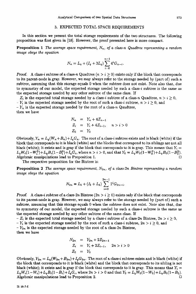
In this section we present the total storage requirements of the two structures. The following proposition was first given in [18]. However, the proof presented here is more compact.

Proposition 1 The average space requirement, N,, of a class-n Quadtree representing a random image obeys the equation

n-1

N, = L, + (Ip + 3L,) c 4iG,_i. i=o

Proof. A class-i subtree of a class-n Quadtree (n > i 2 0) exists only if the block that corresponds to its parent-node is gray. However, we may always refer to the storage needed by (part of) such a subtree, assuming that this storage equals 0 when the subtree does not exist. Note also that, due to symmetry of our model, the expected storage needed by such a class-i subtree is the same as the expected storage needed by any other subtree of the same class. If - Zi is the expected total storage needed by a class-i subtree of a class-n Quadtree, n > i 2 0, - Yi is the expected storage needed by the root of such a class-i subtree, n > i 2 0, and - Y, is the expected storage needed by the root of a class-n Quadtree, then we have

N, = Y, +42,-i

zi = yi+4zi_1, n>i>O

Z-J = Yo

Obviously, Y, = L,(W,,+B,)+I,G,. The root of a class-i subtree exists and is black (white) if the block that corresponds to it is black (white) and the blocks that correspond to its siblings are not all black (white); it exists and is gray if the block that corresponds to it is gray. This means that Yi = L,Wi(l-W~)+L,Bi(l-BQ)+I,Gi, wheren > i > 0, and that Ys = L,Ws(l-W~)+L,Bu(l-Bi). Algebraic manipulations lead to Proposition 1. 0

The respective proposition for the Bintree is:

Proposition 2 The average space requirement, N zn, of a class-2n Bintree representing a random image obeys the equation

2n-1

Nz,, = Ll, + (Lb + Lb) c 2iG2n__i. i=o

Proof. A class-i subtree of a class-2n Bintree (2n > i 2 0) exists only if the block that corresponds to its parent-node is gray. However, we may always refer to the storage needed by (part of) such a subtree, assuming that this storage equals 0 when the subtree does not exist. Note also that, due to symmetry of our model, the expected storage needed by such a class-i subtree is the same as the expected storage needed by any other subtree of the same class. If - Zi is the expected total storage needed by a class-i subtree of a class-2n Bintree, 2n > i 2 0, - Yi is the expected storage needed by the root of such a class-i subtree, 2n > i 2 0, and - Ys,, is the expected storage needed by the root of a class-2n Bintree, then we have

N2n = yzn + 2Z2n-1

Zi = JCi +2Zi-1, 2n>i>O

Z-J = Yo

Obviously, Ysn = L,(W2n+Bsn)+I~G2n. The root of a class-i subtree exists and is black (white) if the block that corresponds to it is black (white) and the block that corresponds to its sibling is not black (white); it exists and is gray if the block that corresponds to it is gray. This means that Yi = L,Wi(l-Wi)+L,Bi(l-Bi)+I,Gi, where 2n > i > 0 and that Ys = L,Wo(l-Wo)+L,Bo(l-Bo). Algebraic manipulations lead to Proposition 2. cl

IS 19:7-E

574 MICHAEL VASSILAKOPOULOS et&.

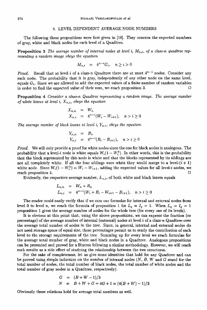
4. LEVEL DEPENDENT AVERAGE NODE NUMBERS

The following three propositions were first given in [18]. They concern the expected numbers of gray, white and black nodes for each level of a Quadtree.

Proposition 3 The average number of internal nodes at level i, A&+, of a class-n quadtree representing a random image obeys the equation

Mn,i = 4”-iGi, n 2 i > 0

Proof Recall that at level i of a class-n Quadtree there are at most 4”-” nodes. Consider any such node. The probability that it is gray, independently of any other node on the same level, equals Gi. Since we are allowed to add the expected values of a finite number of random variables in order to find the expected value of their sum, we reach proposition 3. 0

Proposition 4 Consider a class-n Quadtree representing a random image. The average number of white leaves at level i, Xn,i, obeys the equation

X = w,

Xl:: = 4n9w, - wi+i), n>ikO

The avenge number of brace leaves at level 4, Y=,i, obeys the equation

Y = B,

;); = 4”3Bi - B;+I), n>i>O

Proof. We will only provide a proof for white nodes since the one for black nodes is analogous. The probability that a level-i node is white equals Wi(l - W:). In other words, this is the probability that the block represented by this node is white and that the blocks represented by its siblings are not all completeiy white. If all the four siblings were white they would merge to a level-(i + 1) white node. Since Wi(l - W?) = Wz - W;+I , adding the expected values for all level-i nodes, we reach proposition 4. cl

Evidently, the respective average number, L,,i, of both white and black leaves equals

L 7l,R = W,+&

L,,; =: 4,1i(Wi + Bi - Wi+l - &+I), n > i 2 0

The reader could easily verify that if we sum our formulae for internal and external nodes from level 0 to level n, we reach the formula of proposition 1 for L, = I4 = 1. When L, = 1, = 1 proposition 1 gives the average number of nodes for the whole tree (for every one of its levels).

It is obvious at this point that, using the above propositions, we can express the fraction (or percentage) of the average number of internal (external) nodes at level i of a class-n Quadtree over the average total number of nodes in the tree. Since, in general, internal and external nodes do not need storage space of equal size, these percentages permit us to study the contribution of each level to the storage requirements of the tree. Summing up for every level we reach formulae for the average total number of gray, white and black nodes in a Quadtree. Analogous propositions can be presented and proved for a Bintree following a similar methodology. However, we will reach such results as a side effect of studying the relationship between the two structures.

For the sake of completeness, let us give some identities that hold for any Quadtree and can be proved using simple induction on the number of internal nodes (N, B, W and G stand for the total number of nodes, the total number of black nodes, the total number of white nodes and the total number of gray nodes in a Quadtree, respectively).

G = (B f W - 1)/3

N = ~~W+G=4G+l=(4(~+W)-l)/3

Obviously these relations hold for average total numbers as well.


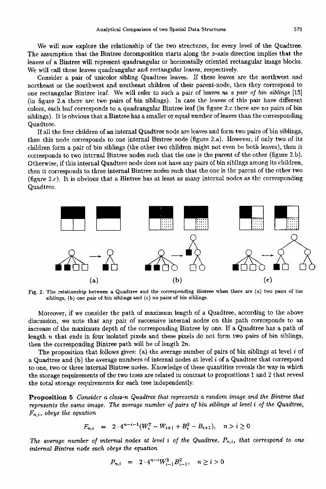
We will now explore the relationship of the two structures, for every level of the Quadtree. The assumption that the Bintree decomposition starts along the z-axis direction implies that the leaves of a Bintree will represent quadrangular or horizontally oriented rectangular image blocks. We will call these leaves quadrangular and rectangular leaves, respectively.

Consider a pair of unicolor sibling Quadtree leaves. If these leaves are the northwest and northeast or the southwest and southeast children of their parent-node, then they correspond to one rectangular Bintree leaf. We will refer to such a pair of leaves as a pair of bin siblings [15] (in figure 2.a there are two pairs of bin siblings). In case the leaves of this pair have different colors, each leaf corresponds to a quadrangular Bintree leaf (in figure 2.c there are no pairs of bin siblings). It is obvious that a Bintree has a smaller or equal number of leaves than the corresponding Quadtree.

If all the four children of an internal Quadtree node are leaves and form two pairs of bin siblings, then this node corresponds to one internal Bintree node (figure 2.a). However, if only two of its children form a pair of bin siblings (the other two children might not even be both leaves), then it corresponds to two internal Bintree nodes such that the one is the parent of the other (figure 2.b). Otherwise, if this internal Quadtree node does not have any pairs of bin siblings among its children, then it corresponds to three internal Bintree nodes such that the one is the parent of the other two (figure 2.~). It is obvious that a Bintree has at least as many internal nodes as the corresponding Quadtree.

Fig. 2: The relationship between a Quadtree and the corresponding Bintree when there are (a) two pairs of bin siblings, (b) one pair of bin siblings and (c) no pairs of bin siblings.

Moreover, if we consider the path of maximum length of a Quadtree, according to the above discussion, we note that any pair of successive internal nodes on this path corresponds to an increase of the maximum depth of the corresponding Bintree by one. If a Quadtree has a path of length n that ends in four isolated pixels and these pixels do not form two pairs of bin siblings, then the corresponding Bintree path will be of length 2n.

The proposition that follows gives: (a) the average number of pairs of bin siblings at level i of a Quadtree and (b) the average numbers of internal nodes at level i of a Quadtree that correspond to one, two or three internal Bintree nodes. Knowledge of these quantities reveals the way in which the storage requirements of the two trees are related in contrast to propositions 1 and 2 that reveal the total storage requirements for each tree independently.

Proposition 5 Consider a class-n Quadtree that represents a random image and the Bintwe that represents the same image. The average number of pairs of bin siblings at level i of the Quadtree, Fn,i, obeys the equation

Fm,i = 2 * 4n-i-1(W~ - Wi+r + Bq - &+I), n > i 2 0

The avenge n~rnbe~ of literal nodes at lever i of the Q~adt~ee, P,+, thut co~spo~d to one internal Bintree node each obeys the eq~at~o~

P n,i = 2 . 4n-iW,f_, Bf__, , n > i > 0

The average number of internal nodes at level i of the Quadtree, R,,,i, that correspond to two internal Bintree nodes each obeys the equation

The average number of internal nodes at level i of the Quadtree, T,,i, that correspond to three internal Bintree nodes obeys the equation

Proof. At level i of the Quadtree there are 2 . 4+6-i rectangular image blocks that represent possible pairs of bin sibbngs. This holds because for every possible level-(i + 1) gray node there are two such blocks. We will call this gray node parent of the two rectangular blocks. The probability that each block of this kind represents a pair of bin siblings [that it consists of unicolor leaves) is: the probabifity that this block consists of two white leaves and the other block which has the same father does not consist of two white leaves, or the proba~ity that this block consists of two black leaves and the other block which has the same father does not consist of two black leaves, that is I@(1 - IV:) + BF(l - B:). Note that we consider the other block having the same father because we must eliminate the case where both blocks consist of unicolor leaves and are replaced by a levei-(i + I) leaf. Since we are allowed to add average values of a finite number of random variables in order to find the average value of their sum, we reach the first formula.

At level S: of the Quadtree there are 4”-; possible gray nodes. Every such node has two rectangular child-blocks which represent possible pairs of bin siblings. The probability that each of these gray nodes corresponds to one internal Bintree node, independently of any other node at the same level, is: the probability that one of its child-blocks is white and the other child-block is black or vice versa, that is lVf_18i_1 + B~_rW~_r. Summing up for every possible level-i gray node we reach the second formula.

The probability that each of these level--i gray nodes corresponds to two internal Entree nodes, independently of any other node at the same level, is: the probability that one of its child-blocks is white or black and the other child-block is not unicolor or vice versa, that is (IV,?_, + BF__,)(l -

II+!-1 - B,2_,) + (1 - W:_r - B:__,)(WiL_r -t-B%,). Ag ain summing up for every possible level-i gray node we reach the third formula,

Lastly, the proba~ity that each of these level-i gray nodes corresponds to three internal Entree nodes, independently of any other node at the same level, is: the probability that both its child- blocks are not unicolor, that is (1 - W&i - Bf__,)2. Again summing up for every possible level-i gray node we reach the last formula. 0

The proposition above can help us form the rate of the average increase (decrease) of internal (external) nodes for each level of a Quadtree when this is converted to a Entree over the total number of internal (external) nodes in the Quadtree. These rates express how (on the average) each level of a Quadtree contributes to the increase or decrease of the memory space required when this tree is converted to a Bintree, if the relative sizes of internal and external nodes are taken into account.

As figure 2 reveaIs, the level-2a Entree leaves correspond to the level-i Quadtree leaves that did not merge, where n > i 2 0. The level-(2i - 1) Bintree leaves correspond to the level-f% - 1) Quadtree leaves that merged, where 7t > i > 0. Thus, setting Fn+ = 0, the average number of level-2i Bintree leaves equals L,,i - 2F,,i, where n 2 i > 0. On the other hand, the average number of level-(2i - 1) Bintree leaves equals F,,;_1, where n 2 i > 0. In addition, figure 2 reveals that the level-2i gray Bintree nodes correspond one to one with the level-i gray Quadtree nodes, where n 2 i > 0. Finally, the level-(2i - I) gray Bintree nodes correspond to the level-i Quadtree nodes that their children do not form two pairs of bin siblings, where n > i > 0. Thus, the average number of level-24 gray Bintree nodes equals P,,i f J& + T%,i (= Mmli) and the average number of level-(2i - 1) gray Bintree nodes equals R,,i + 2T,,;, where n 2 i > 0. Using variations of the formula giving F,,,i that distinguish between black and white nodes and summing up for every Bintree level we can reach formulae for the average total gray, white and black nodes of the Entree. Natur~~y, the same formulae could be reached without using the Quadtree formulae and

Analytica Comparison of two Spatial Data Structures 577

the correspondence formulae. The advantage of the approach we used is that we obtain knowledge about the correspondence itself.

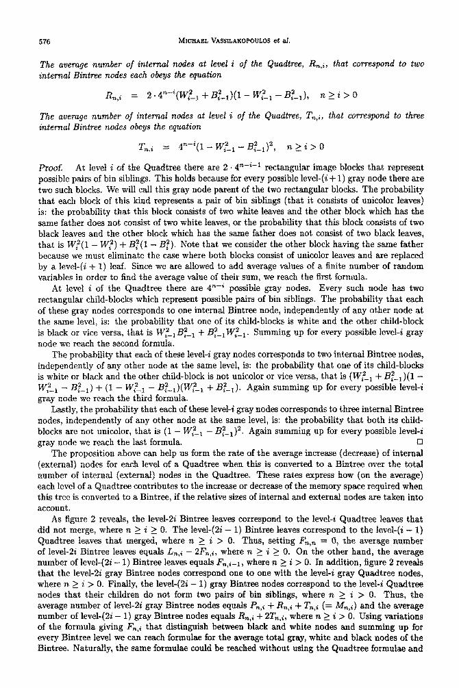
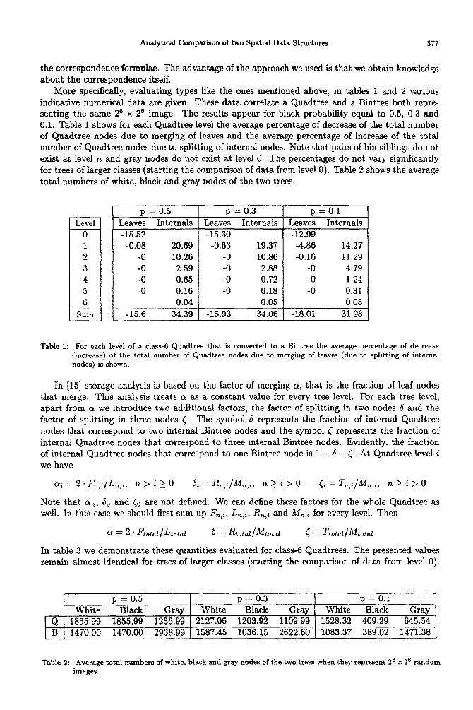
More specifically, evaluating types like the ones mentioned above, in tables 1 and 2 various indicative numerical data are given. These data correlate a Quadtree and a Bintree both representing the same 2s x 26 image. The results appear for black probability equal to 0.5, 0.3 and 0.1. Table 1 shows for each Quadtree level the average percentage of decrease of the total number of Quadtree nodes due to merging of leaves and the average percentage of increase of the total number of Quadtree nodes due to splitting of internal nodes. Note that pairs of bin siblings do not exist at level rz and gray nodes do not exist at level 0. The percentages do not vary significantly for trees of larger classes (stating the comparison of data from level 0). Table 2 shows the average total numbers of white, black and gray nodes of the two trees.

L&l Leaves Internals 0 -15.52 1 -0.08 20.69 2 -0 lo,26 3 -0 2.59 4 -0 0.65 5 -0 0.16 6 0.04

Sum -15.6 34.39

D = 0.5 p = 0.3 P = 0.1 Leaves Internals Leaves Internals -15.30 -12.99

-0.63 19.37 -4.86 14.27 -0 10.86 -0.16 11.29 -0 2.88 -0 4.79 -0 0.72 -0 1.24 -0 0.18 -0 0.31

0.05 0.08 -15.93 34.06 -18.01 31.98

Table 1: For each level of a class-6 Quadtree that is converted to a Bintree the average percentage of decrease (increase) of the total number of Quadtree nodes due to merging of leaves (due to splitting of internal nodes) is shown.

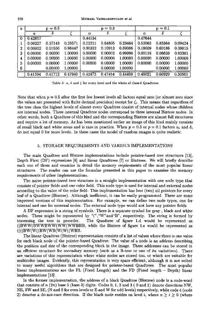
In [15] storage andysis is based on the factor of merging (Y, that is the fraction of leaf nodes that merge. This analysis treats a as a constant value for every tree level. For each tree level, apart from Q we introduce two additionai factors, the factor of splitting in two nodes 6 and the factor of splitting in three nodes f,. The symbol S represents the fraction of internal Quadtree nodes that correspond to two internal Bintree nodes and the symbol < represents the fraction of internal Quadtree nodes that correspond to three internal Bintree nodes. Evidently, the fraction of internal Quadtree nodes that correspond to one Bintree node is 1 - 6 - C. At Quadtree level i we have

clli = 2 1 Fn,i/Ln,i, n > i > 0 & = R+fM,,,i, n 2 i > 0 ci = Tn,i/Mn,i, n > i > 0

Note that cz,, 60 and <O are not defined. We can define these factors for the whole Quadtree as well. In this case we should first sum up F,-+, L,+, Rn,i and &fn,i for every level. Then

o = 2 . ~*t*l/~t~t~i 6 = Rt~t~l/Mt*t~i C = ~~t~i/Mt~t=~

In table 3 we demonstrate these quantities evaluated for class-6 Quadtrees. The presented values remain almost identical for trees of larger classes (starting the comparison of data from level 0).

p = 0.5 p = 0.3 p = 0.1 White Black Gray White Black Gray White Black Gray

. Q 1855.99 1855.99 1236.99 2127.06 1203.92 1109.99 1528.32 409.29 645.54 B 1470.00 1470.00 2938.99 1587.45 1036.15 2622.60 1083.37 389.02 1471.38

Table 2: Average total numbers of white, black and gray nodes of the two trees when they represent 2s x 26 random images.


xl I D = 0.5

a*;857 6 c

0.06227 0.57143 0.28571 0.00002 0.01550 0.98447 0.00000 0.00000 1.00000 0.00000 0.00000 1.00000 0.00000 0.00000 1.00000

0.00000 1.00000

1 0.41594 0.41712 0.47940 0.42473 0.47454 0.44409

p = 0.3

0.4:134 6 c

0.22211 0.64805 0.23464 0.00332 0.10913 0.89086 0.00000 0.00002 0.99998 0.00000 0.00000 1.00000 0.00000 0.00000 1.00000

0.00000 1.00000

P = 0.1

a 6 c 0.47644 0.52063 0.85864 0.09424 0.18009 0.60186 0.39815 0.00118 0.06639 0.93361 0.00000 0.00000 1.00000 0.00000 0.00000 1.00000

0.0~00 1.00000

0.48021 0.66929 0.30501

Table 3: a, 6 and C for every level and the whole of class-6 Quadtrees

Note that when p = 0.5 after the first few lowest levels all factors equal zero (or almost zero since the values are presented with finite decimal precision) except for <is This means that regardless of the tree class the highest levels of almost every Quadtree consist of internal nodes whose children are internal nodes. These internal Quadtree nodes correspond to three internal Bintree nodes. In other words, both a Quadtree of this kind and the corresponding Bintree are almost full structures and require a lot of memory. As has been mentioned earlier an image of this kind mainly consists of small black and white areas and is rare in practice. When p = 0.3 or p = 0.1 factors fyi and 6i do not equal 0 for more levels. In these cases the model of random images is quite realistic.

5. STORAGE REQUIREMENTS AND VARIOUS IMPLEMENTATIONS

The main Quadtree and Bintree implementations include pointer-bred tree structures [13], Depth First (DF) expressions [8] and linear Quadtrees [7] or Bintrees. We will briefly describe each one of them and examine in detail the memory requirements of the most popular linear structures. The reader can use the formulae presented in this paper to examine the memory requirements of other implementations.

The naive pointer-based tree structure is a straight implementation with one node type that consists of pointer fields and one color field. This node type is used for internal and external nodes according to the value of the color field. This implementation has four (two) nil pointers for every leaf of a Quadtree (Bintree). Although inefficient, it can be easily programmed. There are some improved versions of this implementation. For example, we can define two node types, one for internal and one for external nodes. The external node type would not have any pointer fields.

A DF expression is a string of symbols. There is a separate symbol for gray , black and white nodes. These might be represented by “(” ,“W”and”B”, respectively. The string is formed by traversing the tree in preorder. The Quadtree of figure 1.d would be represented as ((BWW(BWWSWW(WW(WWBBB, while the Bintree of figure 1-e would be represented as

((((BW(W((BW(WB(W(W((WBB. The linear Quadtree (Bintree) representation consists of a list of values where there is one value

for each black node of the pointer-bred Quadtree. The value of a node is an address describing the position and size of the corresponding block in the image. These addresses can be stored in an efficient structure for secondary memory (such as a B-tree or one of its variations). There are variations of this representation where white nodes are stored too, or which are suitable for multicolor images. Evidently, this representation is very space efficient, although it is not suited to many useful algorithms that are designed for pointer-based Quadtrees. The most popular linear implementations are the FL (Fixed Length) and the FD (Fixed length - Depth) linear implementations [13].

In the former implementation, the address of a black Quadtree (Bintree) node is a code-word that consists of n (2n) base 5 (base 3) digits. Codes 0, 1, 2 and 3 ( 0 and 1) denote directions NW, NE, SW and SE, (N and S for even levels or E and W for odd levels) respectively, while code 4 (code 2) denotes a do-not-care direction. If the black node resides on level i, where n > i > 0 (where


2n > i 1 0), then the first n - i (2n - i) digits express the directions that constitute the path from

the root to this node and the last i digits are all equal to 4 (2). In the latter implementation, the

address of a black Quadtree (Bintree) node has two parts: the first part is code-word that consists of n (2n) base 4 (base 2) digits. Codes 0, 1, 2 and 3 ( 0 and 1) denote directions NW, NE, SW and SE, (N and S for even levels or E and W for odd levels) respectively. This code-word is formed in a similar way to the code-word of the FL-linear implementation with the difference that the last i digits are all equal to 0. The second part of the address has [logz(n + l)] bits ([logz(2n + l)] bits) and denotes the depth of the black node, or in other words, the number of digits of the first part that express the path to this node. Thus, using FL-linear representation [7, 131, the size of

an address in bits equals ]n . logz(5)] for Quadtrees and [2n * Zogz(3)] for Bintrees, while using FD-linear representation the size of an address in bits equals 2n + [Zogz(n + l)] for Quadtrees and

2n + [Zogz(2n + l)] for Bintrees [13]. The correlation of the space requirements of the two trees depends on the number of external

nodes and on the size of the address values for each tree. Using these representations the four lines of table 4 emerge. The first couple of lines refers to class-6 images, while the second couple of lines

refers to class-9 images. The first line of each couple presents data for FD-linear structures, while the second line of each couple presents data for FL-linear structures. In the case of FD-linear representation, when n = 6, Bintrees excel for black probabilities equal to 50% and 30% while Quadtrees

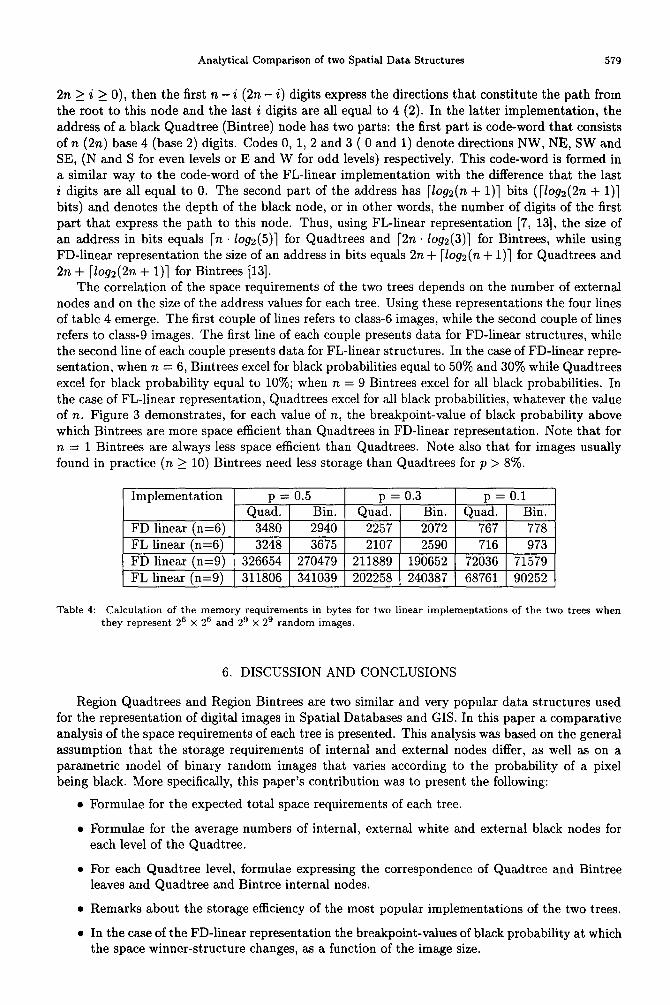
excel for black probability equal to 10%; when n = 9 Bintrees excel for all black probabilities. In the case of FL-linear representation, Quadtrees excel for all black probabilities, whatever the value of n. Figure 3 demonstrates, for each value of n, the breakpoint-value of black probability above

which Bintrees are more space efficient than Quadtrees in FD-linear representation. Note that for n = 1 Bintrees are always less space efficient than Quadtrees. Note also that for images usually found in practice (n 2 10) Bintrees need less storage than Quadtrees for p > 8%.

Table 4: Calculation of the memory requirements in bytes for two linear implementations of the two trees when they represent 2’ x 26 and 2’ x 2’ random images.

6. DISCUSSION AND CONCLUSIONS

Region Quadtrees and Region Bintrees are two similar and very popular data structures used for the representation of digital images in Spatial Databases and GIS. In this paper a comparative analysis of the space requirements of each tree is presented. This analysis was based on the general

assumption that the storage requirements of internal and external nodes differ, as well as on a parametric model of binary random images that varies according to the probability of a pixel being black. More specifically, this paper’s contribution was to present the following:

l Formulae for the expected total space requirements of each tree.

l Formulae for the average numbers of internal, external white and external black nodes for

each level of the Quadtree.

l For each Quadtree level, formulae expressing the correspondence of Quadtree and Bintree leaves and Quadtree and Bintree internal nodes.

l Remarks about the storage efficiency of the most popular implementations of the two trees.

l In the case of the FD-linear representation the breakpoint-values of black probability at which the space winner-structure changes, as a function of the image size.

580 MICHAEL VAWLAKOPOULOS et af.

B 1 0.5

: k 0.4

P r 0.3- *

iz * a 0.2 -

P

* *

* O.l- * * * * *

: 0.0

* * * * * *

I I I I I I I I I I I I I I I I Y 0 1 2 3 4 5 6 7 8 9 10 11 12 13 14 15 16

Class of Quadtree

Fig, 3: For each Quadtree class the corresponding asterisk determines the black probability above which Bintrees are more efficient than Quadtrees in FD-linear representation.

As an example of possible uses of our analysis let us outline the Fully Inverted Quadtree (FI Quadtree [3]). This is a data structure that can be used for storing a set of images or, in other words, an image database, where image pattern searching (also known as content driven retrieval) and fuzzy image pattern searching can be applied. Firstly, a full Quadtree is built, that is a Quadtree where each node has four children, except for the level-0 nodes. As this structure was originally designed 131, each node holds a bit string of m~mum length (the m~mum number of images in the database). Each bit designates a separate image. The block that corresponds to a particular node of the FI-Quadtree is black for every image identified (by a 1) in the bit string of this node. This structure is implemented as a linear Quadtree, kept entirely on secondary memory using a variation of hashing that is suitable for pattern searching. However, due to the large number of 0 bits in the bit strings, a lot of memory space is wasted. The authors of this article are working on an improved inverted Quadtree v~iation where each node holds a list of identifiers only of those images that have the corresponding block black. The resulting structure requires far less memory than the original one.

For this variation, our analysis reveals that

l for almost all practical cases (p > 8% and 7~ 2 10) the use of an inverted FD-linear Bintree in place of the inverted FD-linear Quadtree would lead to significantly lower disk space requirement.

Evidently, other factors like the modification and performance of the pattern searching algorithm should also be examined. In such a study, knowledge of quantitative parameters of different levels might prove helpful.

We can devise variations of the random image model which capture spatial coherence even better and express correlations in coloring between different blocks at the lowest levels. These levels are the ones which play the most important role in the storage behaviour of our structures (statistical data for various applications appear in section 3.2.1.2 of [13]). For example, let us suppose that each level-l image block in a Quadtree is statistically independent to any other level- 1 block in terms of coloring. Let us also suppose that such an image block is black with probability p, white with probability w and gray with probability 1 - p - w. Such a block contains 2 x 2 = 4 pixels and there are 14 different configurations in which it is gray. Thus, we can distinguish 14 different probabilities, one for each different configuration, whose sum is 1 - p - 20. In this way, we can adapt the behaviour of our image in terms of coherence for level-l and level-0 Quadtree blocks, assuming any sort of correlations. Our model for all levels above level 1 does not differ to the original random image model.


The variation of the random image model that we have just described could become even more complex. We may assume that our images obey the random image model for ail Quadtree levels above level 2. That is, each level-2 block is statistically independent to any other level-2 block in terms of coloring, it is black with probability b, white with proba~ity w and gray with probability 1 - p - w, Each level-2 block contains 4 x 4 = 16 pixels and there are 65534 configurations in which this block is gray. Since the number of these configurations is very large, we can group them according to some rule of our choice and assign probabilities to different groups. The sum of all these probabilities must equal 1 - p - M. In this way, we may adapt the behaviour of our image in terms of coherence for level-2, level-l and level-0 Quadtree blocks, assuming any sort of correlations.

The methods of analysis that we present in this article are still of value in these enhanced models, since the original random image model holds for the majority of levels. In addition, the extension of our analysis to the rest of the levels should not be difficult to formulate. The idea behind these enhancements is to customize the coherence behaviour of our image at the most sensitive levels. If the reader decides that such an enhanced model interests him more, then he should study the methods rather than the specific results presented in this paper.

Acknowledgements - The authors would like to thank the anonymous referees for their helpful comments. The first author, who is a postgraduate scholar of the State Scholarship-Foundation of Greece, wishes to thank this foundation for its financial assistance to this research.

F. Arcieri and E. Nardelli. An integration approach to the management of geographical information: CARTECH. Proceedings 2nd Inter. Conf. on Systems Intergration (ICSI), Morristown, New Jersey, 726-737 (1992).

F.W. Burton, V.J. Kollias and J.G. Kollias. Expected and worst-case storage requirements for quadtrees. Pattern Recognition Letters 3 (21, 131-135 (1985).

J.P. Cheiney and A. Tourir. FI-quadtree, a new data structure for content-oriented retrieval and fuzzy search. Proceedings 2nd Symposium on Spatial Databases (SSD), Zurich (1991).

C.R. Dyer. The space efficiency of quadtrees. C~~~~te~ Graphics and Image Pvocessiag 19 (41, 335-348 (1982).

C, Faloutsos. Analytical results on the quadtree d~orn~s~tio~ of arbitrary rectangfes. Pattern Recognition Letters 13 (11, 31-40 (1992),

G.M. Hunter and K. Steiglit. Operations on images using quad trees. IEEE Transactions on Pattern Anuiysis and Machine Intelligence 1 (2), 145-153 (1979).

I. Gargantini. An effective way to represent quadtrees. Communications of the ACM 25 (12), 905-910 (1982).

E. Kawaguchi and T. Endo. On a method of binary picture representation and its application to data com- pression, IElB ~ansact~o~s on Pattern Analysis and Machine Intelligence 3 (l), 27-35 (1980).

R. Laurini and D. Thomson, Fundamentals of Spatial Information Systems. Acudemic Press, London (1992).

F. Olken and D. Rotem. Sampling from Spatial Databases. P~ceed~ngs of the 9th IEEE Data Eng. Conf., 139-208 (1993).

H. Samet, CA. Shaffer, R.C. Nelson, Y.G. Huang, K. Fujimura and A. Rosenfeld. Recent developments in linear quadtree-based geographic information systems. image and Visiola Cornp~t~~g 5 (31, 187-197 (1987).

H. Samet. The design and analysis of spatial data structures. Addison-Wesley, Reading MA (1990).

H. Samet. Applications of spatial data structures: Computer graphics, image processing and GIS, Addison- Wesley, Reading MA (1990).

CA, Sha&r. A formula for computing the number of quadtree node fragments created by a shift. Pattern Reeogni6on Letters 7 (1), 45-49 (1988).

CA. Shaffer, R. Juvvadi and L.S. Heath. A generalized comparison of quadtree and bintree storage requirements. Image and Vision Cornp~t~~g 11 (71, 402-412 (1993).

M. V~silakopouios, Y. Manolopoulos and K. Economou. Overlapping quadtrees for the representation of similar images. fmage and Vision Cornp~t~~g 1X (51, 257-262 (1993).

582 MICXAEL VASSI~KOPO~LOS et ai.

[17] M. Vsssilakopoulos, Y. Manolopoulos and B. Kriill. Efficiency analysis of overlapped quadtress. submitted to Nordic Joumot of Computing.

[18] M. Vassilakopoulos and Y. Manolopoulos. Analytical results on the quadtree storage-requirements. Proceedings

5th inter. conf. on Computer Analysis of Images and Patterns (GAZP), Budapeat, 41-48 (1993).

Documents

ANALYTICAL CO~PA~SO~ OF TWO SPATIAL DATA …delab.csd.auth.gr/papers/IS94vm.pdf · tA preliminary extended abstract of this paper appears in the Proceedings of the 4th Panhellenic