Embed Size (px)
Citation preview
Journal of Civil Engineering and Architecture 11 (2017) 748-756 doi: 10.17265/1934-7359/2017.08.003
Analytical Predictive Models for Lead-Core and
Elastomeric Bearing
Todor Zhelyazov
Technical University of Sofia, Sofia 1000, Bulgaria
Abstract: Constitutive models aimed at predicting the mechanical response of lead-core bearing devices for passive seismic isolation are discussed in this paper. The study is focused on single-degree-of-freedom models which provide a relation between the shear displacement (shear strain) and the shear force (shear stress) in elastomeric and lad-core rubber bearings. Classical Bouc-Wen model along with a numerical procedure for identification of the model constants is described. Alternatively, a constitutive relation introducing a damage variable aimed at assessing the material degradation is also considered.
Key words: Lead core bearing device, constitutive model, analytical models, material degradation.
1. Introduction
Among other strategies to minimize disastrous
effects of seismic activity, the damping devices for
seismic isolation occupy a considerable part. Damping
devices have been used around the world, specifically
in New Zealand, Japan, USA and Italy in the
construction of bridges, large structures and
residential buildings.
The use of seismic isolation results in the reduction
of the peak values of the accelerations generated in a
given structure during earthquake strong motion. The
probability of damage to structural elements, to
nonstructural components and to displacement
sensitive and acceleration sensitive equipment is also
reduced.
According to the generally accepted point of view,
the use of passive seismic isolation aims at shifting
the fundamental natural period of the isolated
structure (compared to the non-isolated) to the long
period range (e.g., 2 to 4 seconds). Technically, this is
achieved by adding horizontally flexible damping
Corresponding author: Todor Zhelyazov, Ph.D.; research fields: numerical modeling and simulation (specifically finite element modeling), mathematical modeling, mechanics of materials (non-linear constitutive laws), earthquake engineering, and mathematical physics. E-mail: [email protected].
devices at the base of the structure in order to
physically decouple it from the ground. Thus, the
vibration of the structure becomes, to some extent,
independent from the ground motion.
The most commonly used types of seismic isolation
devices are elastomeric bearing and friction pendulum
systems. This study is focused on the modeling of the
mechanical response of the first type.
Elastomeric isolators consist of rubber layers
separated by steel shims. The total thickness of the
rubber layers provides the required low horizontal
stiffness of the damping device needed to lengthen the
fundamental natural period of the structure, whereas
the close spacing between the intermediate steel shims
provides large vertical stiffness needed to resist
vertical loads.
The elastomeric isolators can be modified by
adding a lead plug. The modified elastomeric bearing
is often referred to as “LCR (lead-core rubber)
bearing”.
The lead-plug yields relatively quickly under shear
deformation and LCR bearing is then seen to have
well-pronounced hysteresis response under cyclic
loading paths.
The theory that the energy released by a mechanical
system can be evaluated through the work done in
D DAVID PUBLISHING
Analytical Predictive Models for Lead-Core and Elastomeric Bearing
749
hysteresis loops is widely accepted.
The dissipation capacity of LCR bearing is thus
enhanced compared to elastomeric bearing since the
former exhibits a more-pronounced hysteresis
behavior.
Generally, the macroscopic mechanical response of
a LCR bearing is modeled by using a SDOF
(single-degree-of-freedom) constitutive model which
defines the relation between the shear force and the
shear strain. Classical Bouc-Wen [1-3] or rate
independent plasticity model [4] can be used. In some
cases, the time-dependent shear force could be
approximated by the standard two-parameter,
strain-independent Kelvin model (see for example,
Ref. [5]).
LCR devices typically consist of components made
of different materials (lead, rubber and steel)
possessing different mechanical properties. In this
context, SDOF models should provide a
macro-characteristic representative for the mechanical
response of this multiple-component system on the
macro scale.
Constitutive models of LCR bearings have evolved
from simple bi-linear models in which pre-yield
stiffness is simply replaced by the post-yield stiffness
after the yielding in the lead-core, to more
sophisticated models involving differential equations.
Within the scope of this paper, are the Bouc-Wen
model and a macroscopic model in which a damage
variable is introduced.
Original numerical procedures aimed at
implementing these two models are developed by
using the Python software. Elements of a procedure
for curve fitting are also reported.
2. Methods and Materials
This study is aimed at developing numerical
procedures capable of simulating the mechanical
response of elastomeric bearings seen as
single-degree-of-freedom systems. The procedures are
based on widely accepted analytical macroscopic
models. They include appropriate algorithms for
numerical integration and for identification of model
constants.
The identification algorithm is inherently a
sequence of comparisons between the output of the
SDOF model and a target set of data points obtained
experimentally or by finite element analysis.
The prospects of this study include implementation
of the SDOF models in finite element models of
damped structures and definition of coupling rule for
the macroscopic model that should be used in case of
bi-axial loading.
3. Bouc-Wen Model
The Bouc-Wen model consists of an equation that
defines a “skeleton” curve (a relation between shear
displacement and shear force) and another equation
which determines the evolution of the hysteresis
parameter.
The relation between the shear force Q in the LCR
bearing device and the shear displacement u is
obtained by Eq. (1). The evolution of the hysteresis
parameter Z is defined by Eq. (2) (see Refs. [1-3, 6, 7])
as follows:
( ) ZQud
QQ y
y
y αα −+= 1
(1)
( )dt
duAZ
dt
duZZ
dt
du
dt
dZd y +−−= − ηη βγ 1 (2)
where, in Eq. (1), u stands for the current
displacement and Z for a dimensionless hysteresis
component which should satisfy Eq. (2). The other
model constants in Eq. (1) are defined as follows: α is
the post-yielding to pre-yielding stiffness ratio, dy is
the displacement at which the yielding in the lead core
takes place, and Qy is the shear force, corresponding
to the yielding. In Eq. (2), β, γ and A are
dimensionless model constants that are to be
identified by means of curve fiitting; η controls the
transition phase at yielding of the lead core.
Further, the modified mid-point method (see for
Analytical Predictive Models for Lead-Core and Elastomeric Bearing
750
example, Ref. [8]) is used to integrate numerically the
ordinary first-order differential Eq. (2):
( )( )uuZfdt
dZ,= (3)
( )iuZz =0 (4)
( )( )uuZhfzz i ,01 += (5)
( )( )ukhuZhfzz ikk ,211 ++= −+ (k=1,..., n-1) (6)
( ) ( )( )[ ]uHuZhfzzuZ innj ,2
11 +++= − (7)
This is an algorithm to calculate the value of the
function Z at point uj, provided the value at point ui is
known. In Eq. (7), H = uj − ui; n is the number of
substeps into which the interval H is divided. Overdot
denotes a derivative with respect to time. More details
on this algorithm for numerical integration can be
found in Ref. [8].
To solve Eqs. (1) and (2), a numerical procedure is
created in Python software. The algorithm contains a
subroutine for numerical integration by using the
modified mid-point method (Eqs. (3)-(7)).
The output of the model in terms of shear
force-shear displacement curves is presented in Fig. 1.
The model constants that yield these two curves are
summarized in Tables 1 and 2.
4. Constitutive Relation Accounting for Material Degradation
An alternative approach, compared to the model
discussed in the previous section can be found in
Refs. [9-11].
This type of constitutive relations can be situated in
line with models that are compatible with
thermodynamics fundamentals [12].
An internal variable is introduced to assess
mechanical degradation.
Total shear stress is split into three terms: a term
which represents an elastic contribution (τe), and
two terms describing overstresses relaxing in time
(τ1 and τ2):
21 ττττ ++= e (8)
The elastic contribution is evaluated as follows:
)(γτ Fe = (9)
with, F(γ) being a polynomial depending on the shear
strain γ. Shear strain is usually defined as the ratio
between the shear displacement and the total height of
the rubber layers in the bearing device.
Overstresses are defined as functions of the shear
strain, model parameters (E1, E2) and internal
variables (γ1, γ2):
( )111 ,, γγτ EF= (10)
( )222 ,, γγτ EF= (11)
Evolutions of internal variables γv,1 and γv,2 are
determined as follows (see Ref. [9]):
( ) 1,11
1 ,, υτνγγη
γγ
+=
eq
(12)
( )2,2
22 υτν
ηγγγ
+−=
H (13)
where, ν1, η2 and ν2 are model constants. Generally,
they are identified through curve fitting by using
experimental data.
In Eq. (13), H stands for the Heaviside function:
( )
≤>
=00
01
qif
qifqH (14)
As it can be seen in Eq. (12), it is presumed that the
quantity η1 is a function of the shear strain γ, shear strain rate γ and a damage parameter—qe. Damage
parameter supplies information about material
degradation. Upon appropriate calibration on the basis
of the current value of the damage parameter
degrading phenomena in material can be rationally
estimated.
In the present study, the evolution of the damage
parameter is defined by using a governing equation
proposed by Ref. [9]:
Analytical Predictive Models for Lead-Core and Elastomeric Bearing
751
(a)
(b)
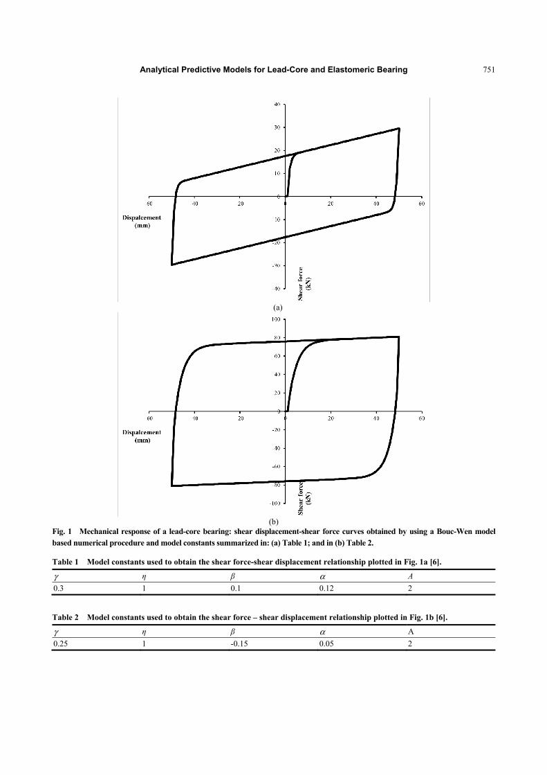
Fig. 1 Mechanical response of a lead-core bearing: shear displacement-shear force curves obtained by using a Bouc-Wen model based numerical procedure and model constants summarized in: (a) Table 1; and in (b) Table 2.
Table 1 Model constants used to obtain the shear force-shear displacement relationship plotted in Fig. 1a [6].
γ η β α A
0.3 1 0.1 0.12 2
Table 2 Model constants used to obtain the shear force – shear displacement relationship plotted in Fig. 1b [6].
γ η β α A
0.25 1 -0.15 0.05 2
Analytical Predictive Models for Lead-Core and Elastomeric Bearing
752
( )
≤≤≤−
=15.00
5.05.0
e
eee qif
qifqq
γγγγζ
(15)
As already stated, damage parameter should enable
the evaluation of the current state of mechanical
damage after a given period of exploitation. The
loading history which has led to the current state of
mechanical degradation is taken into account through
the variable γ—the shear strain and the time rate of
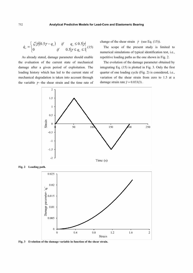
change of the shear strain γ (see Eq. (15)).
The scope of the present study is limited to
numerical simulations of typical identification test, i.e.,
repetitive loading paths as the one shown in Fig. 2.
The evolution of the damage parameter obtained by
integrating Eq. (15) is plotted in Fig. 3. Only the first
quarter of one loading cycle (Fig. 2) is considered, i.e.,
variation of the shear strain from zero to 1.5 at a damage strain rate )3(033.0=γ .
Fig. 2 Loading path.
Fig. 3 Evolution of the damage variable in function of the shear strain.
Analytical Predictive Models for Lead-Core and Elastomeric Bearing
753
5. Identification of the Model Parameters
The numerical procedure employed for the
identification of model constants is outlined in this
section. The identification procedure is based on
genetic algorithm [13].
Curve fitting generally consists in finding a set of
model parameters for which the results obtained by
implementing the model fits best a target set of data
points. Generally, the target set is an experimentally
obtained relation that characterizes behavior of the
modeled mechanical system. Alternatively, the target
set of data points can be defined on the basis of results
obtained by finite element analysis.
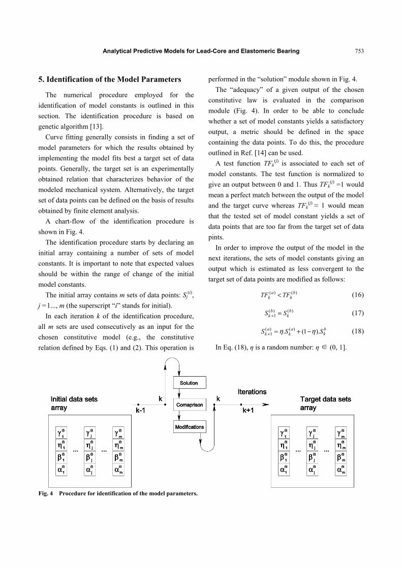
A chart-flow of the identification procedure is
shown in Fig. 4.
The identification procedure starts by declaring an
initial array containing a number of sets of model
constants. It is important to note that expected values
should be within the range of change of the initial
model constants.
The initial array contains m sets of data points: Sj(i),
j =1..., m (the superscript “i” stands for initial).
In each iteration k of the identification procedure,
all m sets are used consecutively as an input for the
chosen constitutive model (e.g., the constitutive
relation defined by Eqs. (1) and (2). This operation is
performed in the “solution” module shown in Fig. 4.
The “adequacy” of a given output of the chosen
constitutive law is evaluated in the comparison
module (Fig. 4). In order to be able to conclude
whether a set of model constants yields a satisfactory
output, a metric should be defined in the space
containing the data points. To do this, the procedure
outlined in Ref. [14] can be used.
A test function TFk(j) is associated to each set of
model constants. The test function is normalized to
give an output between 0 and 1. Thus TFk(j) =1 would
mean a perfect match between the output of the model
and the target curve whereas TFk(j) ≈ 1 would mean
that the tested set of model constant yields a set of
data points that are too far from the target set of data
pints.
In order to improve the output of the model in the
next iterations, the sets of model constants giving an
output which is estimated as less convergent to the
target set of data points are modified as follows:
)()( bk
ak TFTF < (16)
)()(1
bk
bk SS =+ (17)
bk
ak
ak SSS ).1(. )()(
1 ηη −+=+ (18)
In Eq. (18), η is a random number: η ∈ (0, 1].
Fig. 4 Procedure for identification of the model parameters.
Analytical Predictive Models for Lead-Core and Elastomeric Bearing
754
There are two ways to define a criterion for
termination of the procedure. Either the maximum
number of iterations can be limited to a predefined
value or an acceptable value of the test function can
be set at the beginning of the procedure.
Finally, from the target array of sets )(t
jS (superscript “t” stands for target), the one yielding
an optimal fit with the experimental data can be chosen.
(a) (b)
(c) (d)
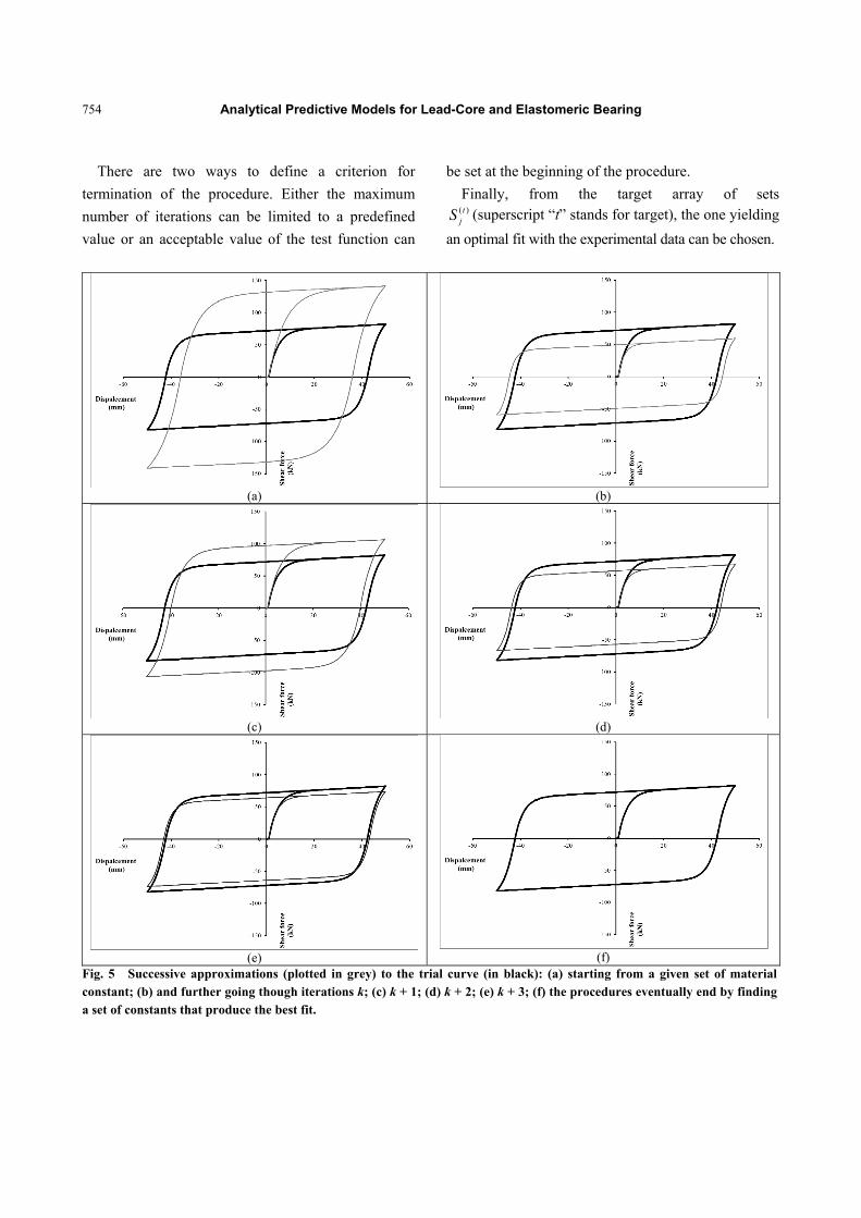
(e) (f) Fig. 5 Successive approximations (plotted in grey) to the trial curve (in black): (a) starting from a given set of material constant; (b) and further going though iterations k; (c) k + 1; (d) k + 2; (e) k + 3; (f) the procedures eventually end by finding a set of constants that produce the best fit.
Analytical Predictive Models for Lead-Core and Elastomeric Bearing
755
The implementation of the identification procedure
is illustrated by choosing a target set of data points.
Several steps of the identification procedure are
shown in Figs. 5a-5f.
The target curve is plotted in black whereas the best
approximation for a given step of the curve fitting
procedure—in grey. It can be seen that the “best
guess” for a given iteration is getting closer to the
target data set with the progress of the curve fitting
procedure.
6. Concluding Remarks
Analytical models aimed at reproducing the
mechanical response of lead-core rubber and
elastomeric bearings for passive seismic isolation
have been discussed in this paper.
Numerical procedures have been developed by
using Python software. These procedures have been
created on the basis of models proposed in literature,
namely the classical Bouc-Wen model and a
constitutive relation that takes into account the
mechanical degradation in an elastomeric bearing.
A curve fitting algorithm has also been presented.
The procedure for identification of the model
constants is based on genetic algorithms. Generally,
identification is made through comparison with
experimental data. The author believes that
identification of single-degree-of-freedom constitutive
models can be also performed by using data obtained
by finite element analysis. The latter option might
optimize the time-demanding and expensive
experimental research program. However, it should be
noted that the study outlined in this paper has to be
completed by experimental tests on damping devices.
The proposed numerical procedures are to be
subsequently integrated in the finite element analyses
of damped structures to account for the effect of the
seismic isolators. However, before implementing the
discussed procedures in finite element models of
structures, a coupling rule should be defined for the
case of bi-axial loading.
Acknowledgments
This paper is a result of a continuous collaboration
with the Earthquake Engineering Research Centre, a
part of the University of Iceland, started in 2013.
References
[1] Bouc, R. 1967. “Forced Vibration of Mechanical Systems with Hysteresis.” In Proceedings of the Fourth Conference on Nonlinear Oscillation, Prague, Czechoslovakia, 315.
[2] Bouc, R. 1971. “Mathematical Model of Hysteresis: Application in Single-Degree-of-freedom Systems.” Acustica 24: 16-25.
[3] Wen, Y. K. 1976. “Method of Random Vibration of Hysteretic System.” J. Eng. Mechanics Division ASCE 102 (2): 249-63.
[4] Nagarajaiah, S., Reinhorn, A. M., and Constantinou, M. C. 1991. “Nonlinear Dynamic Analysis of 3-D-base-Isolated Structures.” J. Struct. Eng. 117: 2035-54.
[5] Chang, S., Makris, N., Whittaker, A. S., and Thompson, A. C. T. 2002. “Experimental and Analytical Studies on the Performance of Hybrid Isolation Systems.” Earthquake Engng Struct. Dyn. 31: 421-43.
[6] Constantinou, M. C., and Tadjbakhsh, M. 1985. “Hysteretic Dampers in Base Isolation: Random Approach.” Journal of Structural Eng. 111 (4): 705-21.
[7] Song, J., and Der Kiureghian, A. 2006. “Generalized Bouc-Wen Model for Highly Asymmetric Hysteresis.” J. Eng. Mechanics ASCE 132 (6): 610-8.
[8] Press, W. H., Teukolsky, S. A., Vetterling, W. T., and Flannery, B. P. 2007. Numerical Recipies, The Art of Scientific Computing. 3rd ed. Cambridge: Cambridge University Press.
[9] Dall’Astra, A., and Ragni, L. 2006. “Experimental Tests and Analytical Model of High Damping Rubber Dissipating Devices.” Engineering Structures 28 (13): 1874-84.
[10] Govindjee, S., and Simo, J. C. 1992. “Mullins Effect and the Strain Amplitude Dependence of the Storage Modulus.” Int. J. Solids Struct. 29: 1737-51.
[11] Haupt, P., and Sedlan, H. 2001. “Viscoplasticity of Elastomeric Materials: Experimental Facts and Constitutive Modelling.” Arch. Appl. Mech. 71: 89-109.

Analytical Predictive Models for Lead-Core and Elastomeric Bearing
756
[12] Fabrizio, M., and Morro, A. 1992. Mathematical Problems in Linear Viscoelasticity. Philadelphia: SIAM—Studies In Applied Mathematics.
[13] Goldberg, D. E. 1989. Genetic Algorithms in Search, Optimization and Machine Learning. Reading (MA):
Addison-Wesley. [14] Kwok, N. M., Ha, Q. P., Nguyen, M. T., Li, J., and
Samali, B. 2007. “Bouc-Wen Model Parameter Identification for a MR Fluid Damper Using Computationally Efficient GA.” ISA Trans. 46 (2): 167-79.