Analyzing BSE surveillance in low prevalence countries

Short communication

Analyzing BSE surveillance in low prevalence

countries§

Mark Powell a,*, Aaron Scott b, Eric Ebel b

a U.S. Department of Agriculture, Office of Risk Assessment and Cost Benefit Analysis,

1400 Independence Avenue, SW, Rm. 4032 (MS 3811), Washington, DC 20250, United Statesb U.S. Department of Agriculture, Animal and Plant Health Inspection Service,

2150 Centre Avenue, Building B, Mail Stop 2E7, Fort Collins, CO 80526, United States

Received 10 May 2007; received in revised form 24 August 2007; accepted 21 September 2007

Abstract

If the prevalence of bovine spongiform encephalopathy (BSE) varies among cohorts within a population,

stratified analysis of BSE surveillance data may allow identification of differences in BSE exposure that are

important with respect to the design and evaluation of disease prevention and control measures. In low BSE

prevalence populations, however, surveillance at levels that meet or exceed international guidelines may

provide insufficient statistical power to distinguish prevalence levels among cohorts. Furthermore, over-

stratification to account for hypothetical variability in the population may inflate uncertainty in BSE risk

estimates.

Published by Elsevier B.V.

Keywords: Bovine spongiform encephalopathy; Prevalence; Surveillance; Risk assessment

1. Introduction

If the prevalence of bovine spongiform encephalopathy (BSE) varies substantially among

cohorts within a population, stratified analysis of BSE surveillance data may allow detection of

differences in BSE exposure that are important with respect to the design and evaluation of

www.elsevier.com/locate/prevetmed

Available online at www.sciencedirect.com

Preventive Veterinary Medicine 83 (2008) 337–346

§ The opinions expressed herein are the views of the author and do not necessarily reflect the official policy or position

of the U.S. Department of Agriculture. Reference herein to any specific commercial products, process, or service by trade

name, trademark, manufacturer, or otherwise, does not necessarily constitute or imply its endorsement, recommendation,

or favoring by the United States Government.

* Corresponding author. Tel.: +1 202 720 9786; fax: +1 202 720 1815.

E-mail address: [email protected] (M. Powell).

0167-5877/$ – see front matter. Published by Elsevier B.V.

doi:10.1016/j.prevetmed.2007.09.003

mailto:[email protected]

http://dx.doi.org/10.1016/j.prevetmed.2007.09.003

disease prevention and control measures. In this regard, the European Food Safety Authority

(EFSA) states, ‘‘[t]he ultimate means of determining the effectiveness of [BSE] controls is to

estimate the prevalence of infection within birth cohorts before and after the introduction of the

interventions’’ (EFSA, 2006, p. 29). At low BSE prevalence levels, however, national animal

health surveillance at levels exceeding international guidelines provide limited power to

statistically distinguish differences in prevalence among cohorts, defined by birth years or

otherwise.

Stratified analysis of animal health surveillance data can yield more precise and useful

disease prevalence estimates if the stratification variables account for much of the observed

variability in the population. However, poor stratification may result in lower precision of the

estimated population parameter than simple random sampling when the variance within strata

exceeds the variance between strata (Cochran, 1977). Any variance reduction achieved by

stratification also must more than compensate for the lost degree of freedom for each stratum.

For a fixed sample size, too many strata (overstratification) produces sparseness of data within

strata. This may limit statistical power to detect differences among strata and result in strata with

zero cases.

Separating uncertainty due to lack of knowledge and variability due to random or systematic

heterogeneity also has been promoted as a principle of good risk assessment (Bogen and Spear,

1987; Burmaster and Anderson, 1994; Hoffman and Hammonds, 1994). (See Murray (2002) for

an introduction to second-order modeling separating uncertainty and variability in animal health

risk analysis.) At least in principle, the prevalence of disease in a population has distinct

uncertainty and variability dimensions. Prevalence has a true but unknown value at a specific time

and location, and prevalence may vary over time and among subpopulations, regions, etc.

However, there may be empirical limitations on the extent to which uncertainty and variability

can be disentangled; for example, when variation occurs at a scale smaller than the uncertainty

due to measurement error (Baecher, 1999).

The objectives of this paper are to evaluate the statistical power of national BSE surveillance

at levels meeting or exceeding international guidelines and to illustrate that overstratification to

account for hypothetical variability in the population may inflate uncertainty in BSE risk

estimates.

2. Methods

This section begins with a description of the methods used for statistical power analysis. Two

scenario analyses were used to evaluate the statistical power of national BSE surveillance at

levels meeting or exceeding international guidelines to statistically distinguish differences in

prevalence between birth cohorts. A final scenario illustrates that overstratification to account for

hypothetical variability of BSE prevalence within a cattle population may inflate uncertainty in

the estimated probability of drawing BSE-infected cattle in two-stage sampling when animals are

sampled from a randomly selected cohort.

2.1. Statistical power analysis for two independent prevalence samples

The power of a statistical test is the probability of rejecting the null hypothesis (H0) when it is

false. The power depends on the test level of significance (a), the magnitude of effect or

difference (d) under the alternative hypothesis (Ha), sample size (n), and variability in the

population (s2).

M. Powell et al. / Preventive Veterinary Medicine 83 (2008) 337–346338

Let:

� pi = true, unknown disease prevalence in a large population with i = 1, 2

� ni = ith random sample size

� a = p (reject true H0)

� b = p (not reject false H0)

� power (1 � b) = p (reject false H0)

Under the scenarios considered here, we specify:

� H0: p1 � p2 = 0

� Ha: p1 � p2 = d

and assume n1 = n2 for simplicity.

Assuming a constant probability of disease, the number of cases (c) in a sample (n) from the

population varies among random draws according to the binomial distribution:

c�Binomialðn; pÞwhere c = 0, 1, . . ., n; n = random sample size and p = disease prevalence.

The prevalence uncertainty distribution is assumed to follow a beta distribution, the conjugate

prior to the binomial probability parameter (Rice, 1988):

p�Beta ða; bÞ

where p ¼ a=aþ b and s2p ¼ ab=ðaþ bÞ2ðaþ bþ 1Þ are the estimators of p and s2

p, respec-

tively.

For c > 0, the beta distribution parameters may be estimated using the method of matching

moments (Evans et al., 1993):

a ¼ p

��pð1� pÞ

s2p

�� 1

�

b ¼ ð1� pÞ��

pð1� pÞs2

p

�� 1

�

where p ¼ c=n and s2p ¼ pð1� pÞ=ðn� 1Þ.

For c = 0, however, the matching moments estimates cannot be obtained. (Estimating the beta

distribution parameters would involve dividing by zero because the sample variance is zero.) To

permit estimation of prevalence for samples with c = 0, we estimate the beta distribution

parameters assuming a uniform prior on p (Rice, 1988):

pposterior ¼ Betaðcþ aprior; n� cþ bpriorÞwhere pprior = Beta(aprior, bprior) = Beta(1,1) = Uniform(0,1); a ¼ cþ 1; b ¼ n� cþ 1.

The test statistic for comparing two independent prevalence samples is (Rice, 1988):

z ¼ ð p1 � p2Þ � ð p1 � p2Þs p1� p2

where s p1� p2¼

ffiffiffiffiffiffiffiffiffiffiffiffiffiffiffiffiffiffiffiffis2

p1þ s2

p2

q.

M. Powell et al. / Preventive Veterinary Medicine 83 (2008) 337–346 339

Under H0: p1 � p2 = 0. Under Ha: p1 � p2 = d. As a consequence of the asymmetric sampling

distribution of the z statistic under the alternative hypothesis in low prevalence applications,

conventional estimation methods overstate the sample size needed to detect a difference between

two populations with a specified significance level and power (Williams et al., 2007). Here,

however, we make the simplifying assumption that the standard normal (z � N(0,1)) approximation

is sufficient to assess the power of a test to distinguish prevalence levels between cohorts in low BSE

prevalence countries. The impact of this standard simplifying assumption is to underestimate the

statistical power for a fixed sample size, the degree of underestimation depending on p1 and d.

By convention, we set a = 0.05 for a two-tailed significance test. (A two-tailed test considers

that prevalence may increase or decrease relative to a baseline.) Therefore, the power of the test

under Ha: p1 � p2 = d is approximated by (Rice, 1988):

ð1� bÞ � 1�F

�1:96� d

s p1� p2

�þF

�� 1:96� d

s p1� p2

�

where F = standard normal cumulative distribution function.

For fixed n, the statistical power expression can be evaluated as a function of d. Other things

being equal, the greater the difference in prevalence between two populations, the greater the

power of the test.

2.2. Scenario 1—OIE guidelines for BSE surveillance

Scenario 1 is intended to illustrate the statistical power of national BSE surveillance

satisfying, but not exceeding, international guidelines. The approach used under the World

Organization for Animal Health (OIE) Guidelines for BSE Surveillance assigns ‘point values’ to

each sample that reflect the likelihood of detecting infected cattle within broadly defined

surveillance strata (OIE, 2006, Appendix 3.8.4).

Alternatively, countries may use a more refined statistical model, such as the European Union

(EU) BSurvE model (Wilesmith et al., 2004, 2005; Prattley et al., 2007) to estimate the random

sample size equivalent of targeted BSE surveillance data. Under BSurvE, one BSE surveillance

point is estimated to be equivalent to an animal randomly selected for testing from the national

herd using a perfect diagnostic test. BSurvE uses a country’s epidemiologic information to

predict parameters such as incubation period of BSE, probable length of an infected animal’s life,

and the dynamics of disease expression in infected animals. Because this information is

unavailable in countries that have observed few or no BSE cases, default values based on

European data provide useful surrogates. BSurvE combines this epidemiologic information with

country-specific demographic information about a national herd (size and age distribution) and

national BSE surveillance data to obtain a set of point values for samples taken from cattle of

different age and surveillance streams—healthy slaughter, fallen stock, casualty slaughter, or

clinical suspect. The points represented by an animal tested for BSE are based on the relative

likelihood that the disease would be detected in an animal leaving the herd at a particular age and

by a particular surveillance stream.

The OIE Guidelines for BSE Surveillance (Type A) call for countries to accumulate 300,000

BSE surveillance points over seven consecutive years to achieve a nominal design prevalence of

one case per 100,000 in the adult cattle population at a confidence level of 95% (OIE, 2006,

Appendix 3.8.4). Assuming the binomial distribution with zero cases observed in a random sample:

1� ð1� pdÞn ¼ CL


where pd (design prevalence) = 1 � 10�5; n (random sample size) = 300,000; CL (confidence

level) = 0.95.

Thus, the OIE BSE surveillance points target is based on an apparent design prevalence that

equates to true disease prevalence under the assumption of perfect test sensitivity and specificity.

BSurvE input parameters allow the user to adjust the estimated random sample size equivalent to

account for less than perfect test sensitivity. Under the default setting, BSurvE assumes that test

sensitivity is 100% for clinical animals, 40% within 1 year prior to the onset of clinical BSE

symptoms, and zero if sampling occurs more than 1 year prior to clinical onset.

To simplify the scenario analysis, assume that over a period of seven consecutive years, a

national BSE surveillance program accumulates the equivalent of n = 42,857 random samples

per birth year cohort, adjusted to account for an imperfect test, to estimate true BSE prevalence.

Note that the case of zero infected animals in a cohort sample presents a threshold for prevalence,

which we specify as p0. By convention, we solve for the minimum difference in prevalence

(d = p1 � p0) under the alternative hypothesis such that the power of the test (1 � b) � 80% (i.e.,

b < 0.2).

2.3. Scenario 2—diminished power in low prevalence populations

Scenario 2 considers sampling at levels far exceeding the OIE guidelines for BSE surveillance

and illustrates the diminished statistical power of sampling to detect substantial differences in

prevalence in low prevalence populations. Consider two hypothetical countries that have

accumulated 1 million BSE surveillance points (random sample equivalents) for each of two

birth cohorts. Under this scenario, the birth cohorts may represent multiple birth years, such as

animals born before and after introduction of a ruminant-to-ruminant feed ban. The two countries

differ, however, with respect to their initial prevalence. Assume that the initial prevalence in

‘‘Country A’’ is 1 per 10,000, while that in ‘‘Country B’’ is 1 per 100,000. Under this scenario, we

calculate the power of the sampling in each hypothetical country to detect a 50% decline in BSE

prevalence between cohort 1 and cohort 2. Because this scenario does not require estimation of

prevalence for samples with zero cases, we simplify the analysis by using the maximum

likelihood estimate of prevalence ( p = c/n).

2.4. Scenario 3—overstratification inflates uncertainty in BSE risk estimates

Spatial and temporal overdispersion (clustering) of a hazardous agent may result in ‘‘hot

spots’’ and/or ‘‘hot moments’’ of risk greater than predicted under the assumption of random

variation about a constant mean level. FAO/WHO (2003, p. 23) recommends that clustering of

pathogens in food and water ‘‘must be taken into account when estimating health risks.’’ In an

animal health risk context, for example, feedlot cattle are likely to be processed as a group, or

producers may contract with suppliers from a particular region. Animal health risk estimates that

account for this non-random mixing of animals may be impacted by extra-binomial variability

due to heterogeneity in the prevalence of infection among subpopulations. However, a cohort of

animals may be defined by any number of common characteristics, and cattle cohorts may or may

not represent distinct subpopulations with respect to BSE prevalence.

Scenario 3 illustrates how overstratification to account for hypothetical variability of BSE

prevalence within a cattle population may inflate uncertainty in the estimated probability of

drawing BSE-infected cattle in two-stage sampling when animals are sampled from a randomly

selected cohort. Assume that a large cattle population consists of 12 cohorts (defined by 4


geographic regions and 3 market classes) of equal size. BSE prevalence estimates are based on

300,000 random sample equivalents evenly distributed among the 12 cohorts:

� n ¼Pk

i¼1 ni ¼ 300; 000, with k = 12 and ni = 25,000 for all i

� wi ¼ proportion of animals in the ith cohort ¼ 1=k ¼ 1=12

Assume a total of 60 cases are observed:

c ¼X

ci ¼ 60

In setting up Scenario 3, the number of cases per cohort (ci) was obtained by drawing random

values from a binomial distribution with a fixed prevalence of 2 � 10�4:

ci�Binomialð25; 000; 2� 10�4Þ

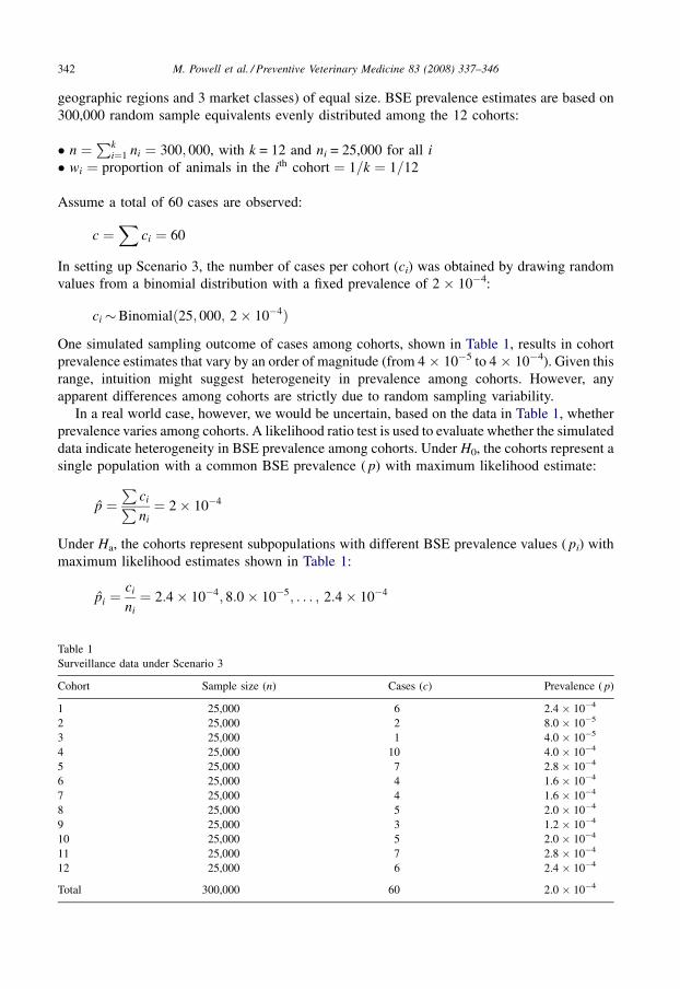
One simulated sampling outcome of cases among cohorts, shown in Table 1, results in cohort

prevalence estimates that vary by an order of magnitude (from 4 � 10�5 to 4 � 10�4). Given this

range, intuition might suggest heterogeneity in prevalence among cohorts. However, any

apparent differences among cohorts are strictly due to random sampling variability.

In a real world case, however, we would be uncertain, based on the data in Table 1, whether

prevalence varies among cohorts. A likelihood ratio test is used to evaluate whether the simulated

data indicate heterogeneity in BSE prevalence among cohorts. Under H0, the cohorts represent a

single population with a common BSE prevalence ( p) with maximum likelihood estimate:

p ¼P

ciPni¼ 2� 10�4

Under Ha, the cohorts represent subpopulations with different BSE prevalence values ( pi) with

maximum likelihood estimates shown in Table 1:

pi ¼ci

ni¼ 2:4� 10�4; 8:0� 10�5; . . . ; 2:4� 10�4


Table 1

Surveillance data under Scenario 3

Cohort Sample size (n) Cases (c) Prevalence ( p)

1 25,000 6 2.4 � 10�4

2 25,000 2 8.0 � 10�5

3 25,000 1 4.0 � 10�5

4 25,000 10 4.0 � 10�4

5 25,000 7 2.8 � 10�4

6 25,000 4 1.6 � 10�4

7 25,000 4 1.6 � 10�4

8 25,000 5 2.0 � 10�4

9 25,000 3 1.2 � 10�4

10 25,000 5 2.0 � 10�4

11 25,000 7 2.8 � 10�4

12 25,000 6 2.4 � 10�4

Total 300,000 60 2.0 � 10�4

The likelihood ratio is given by

L ¼Q

iBinomialð pjci; niÞQiBinomialð pijci; niÞ

The likelihood ratio test statistic is �2 log L. With k = 12 strata (cohorts) and k � 1 degrees of

freedom (d.f.), the distribution of �2 log L under the null hypothesis is chi-square with d:f: ¼11 x2

11

� �(Rice, 1988).

If we fail to reject the null hypothesis, we would correctly assume that the cohorts have the

same prevalence, estimated by p. However, we can evaluate the effect on the risk estimate of

accounting for hypothetical variability by assuming that the cohorts have different prevalence

values, estimated by pi.

Under the assumption of heterogeneous prevalence, we simulate the probability of drawing a

number of BSE-infected animals (cg) when a group of 25,000 cattle is sampled from a randomly

selected cohort:

cg�Binomialð25; 000; pcÞ

where pc is the mixing distribution in which equal weights ðw1; . . . ;w12 ¼ 1=12Þ are given to the

cohort prevalence estimates ð p1; . . . ; p12Þ, and pi�Betaðai; biÞ.Under the assumption of homogeneous prevalence:

cg�Binomialð25; 000; pÞ

where p�Betaða; bÞ, with a and b estimated based on c = Sci and n = Sni using the method of

matching moments.

Because ci > 0 for all cohorts, there is no need to specify a prior on prevalence.

Therefore, Betaðai; biÞ and Betaða; bÞ were estimated using the method of matching

moments described above. Monte Carlo methods were used to estimate the probability

distribution of the number of BSE-infected animals in a group of 25,000 cattle under both

assumptions (heterogeneous and homogeneous prevalence). A one-dimensional Monte Carlo

simulation was performed that treats random sampling variability as an a priori uncertainty

distribution for a sample drawn from the population. Monte Carlo simulation was performed

(50,000 iterations) using Palisades# @RiskTM (Ver. 4.5), an add-on to Microsoft# ExcelTM

(2003).

3. Results

3.1. Scenario 1—OIE guidelines for BSE surveillance

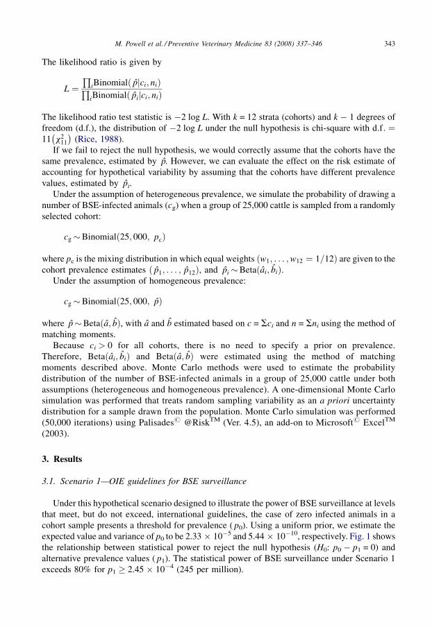
Under this hypothetical scenario designed to illustrate the power of BSE surveillance at levels

that meet, but do not exceed, international guidelines, the case of zero infected animals in a

cohort sample presents a threshold for prevalence ( p0). Using a uniform prior, we estimate the

expected value and variance of p0 to be 2.33 � 10�5 and 5.44 � 10�10, respectively. Fig. 1 shows

the relationship between statistical power to reject the null hypothesis (H0: p0 � p1 = 0) and

alternative prevalence values ( p1). The statistical power of BSE surveillance under Scenario 1

exceeds 80% for p1 � 2.45 � 10�4 (245 per million).


3.2. Scenario 2—diminished power in low prevalence populations

Under this scenario, sampling levels far exceed the OIE Guidelines for BSE Surveillance. At a

5% significance level, the power of the surveillance in Country A (initial prevalence of 1 per

10,000) to detect a 50% decline in BSE prevalence between two cohorts is 98%. In comparison,

the corresponding power of the surveillance in Country B (initial prevalence of 1 per 100,000) to

detect a 50% decline in BSE prevalence between cohorts is 25%. In Country B, an order of

magnitude decline (from 10�5 to 10�6) would be required for the power of the surveillance under

Scenario 2 to approach the conventional minimum statistical power criterion of 80%. Of course,

the diminished power of the surveillance to detect changes in low prevalence populations also

applies to increases in prevalence. At a 5% significance level, the surveillance in Country A

provides a power of 80% to detect an increase a 44% increase in prevalence (from 1 � 10�4 to

1.44 � 10�4). In Country B, a prevalence increase of 170% (from 1 � 10�5 to 2.7 � 10�5) would

be required.

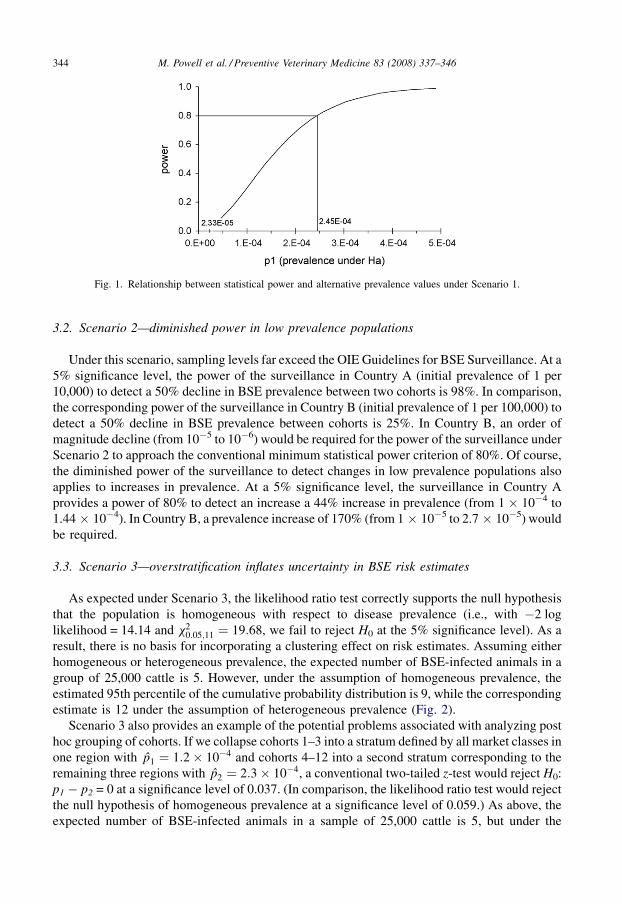
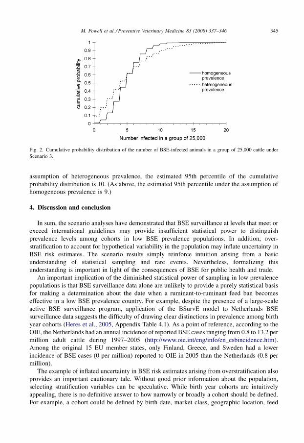
3.3. Scenario 3—overstratification inflates uncertainty in BSE risk estimates

As expected under Scenario 3, the likelihood ratio test correctly supports the null hypothesis

that the population is homogeneous with respect to disease prevalence (i.e., with �2 log

likelihood = 14.14 and x20:05;11 ¼ 19:68, we fail to reject H0 at the 5% significance level). As a

result, there is no basis for incorporating a clustering effect on risk estimates. Assuming either

homogeneous or heterogeneous prevalence, the expected number of BSE-infected animals in a

group of 25,000 cattle is 5. However, under the assumption of homogeneous prevalence, the

estimated 95th percentile of the cumulative probability distribution is 9, while the corresponding

estimate is 12 under the assumption of heterogeneous prevalence (Fig. 2).

Scenario 3 also provides an example of the potential problems associated with analyzing post

hoc grouping of cohorts. If we collapse cohorts 1–3 into a stratum defined by all market classes in

one region with p1 ¼ 1:2� 10�4 and cohorts 4–12 into a second stratum corresponding to the

remaining three regions with p2 ¼ 2:3� 10�4, a conventional two-tailed z-test would reject H0:

p1 � p2 = 0 at a significance level of 0.037. (In comparison, the likelihood ratio test would reject

the null hypothesis of homogeneous prevalence at a significance level of 0.059.) As above, the

expected number of BSE-infected animals in a sample of 25,000 cattle is 5, but under the


Fig. 1. Relationship between statistical power and alternative prevalence values under Scenario 1.

assumption of heterogeneous prevalence, the estimated 95th percentile of the cumulative

probability distribution is 10. (As above, the estimated 95th percentile under the assumption of

homogeneous prevalence is 9.)

4. Discussion and conclusion

In sum, the scenario analyses have demonstrated that BSE surveillance at levels that meet or

exceed international guidelines may provide insufficient statistical power to distinguish

prevalence levels among cohorts in low BSE prevalence populations. In addition, over-

stratification to account for hypothetical variability in the population may inflate uncertainty in

BSE risk estimates. The scenario results simply reinforce intuition arising from a basic

understanding of statistical sampling and rare events. Nevertheless, formalizing this

understanding is important in light of the consequences of BSE for public health and trade.

An important implication of the diminished statistical power of sampling in low prevalence

populations is that BSE surveillance data alone are unlikely to provide a purely statistical basis

for making a determination about the date when a ruminant-to-ruminant feed ban becomes

effective in a low BSE prevalence country. For example, despite the presence of a large-scale

active BSE surveillance program, application of the BSurvE model to Netherlands BSE

surveillance data suggests the difficulty of drawing clear distinctions in prevalence among birth

year cohorts (Heres et al., 2005, Appendix Table 4.1). As a point of reference, according to the

OIE, the Netherlands had an annual incidence of reported BSE cases ranging from 0.8 to 13.2 per

million adult cattle during 1997–2005 (http://www.oie.int/eng/info/en_esbincidence.htm).

Among the original 15 EU member states, only Finland, Greece, and Sweden had a lower

incidence of BSE cases (0 per million) reported to OIE in 2005 than the Netherlands (0.8 per

million).

The example of inflated uncertainty in BSE risk estimates arising from overstratification also

provides an important cautionary tale. Without good prior information about the population,

selecting stratification variables can be speculative. While birth year cohorts are intuitively

appealing, there is no definitive answer to how narrowly or broadly a cohort should be defined.

For example, a cohort could be defined by birth date, market class, geographic location, feed


Fig. 2. Cumulative probability distribution of the number of BSE-infected animals in a group of 25,000 cattle under

Scenario 3.

http://www.oie.int/eng/info/en_esbincidence.htm

source, and other attributes. For a given level of surveillance, as cohorts are more narrowly

defined, the sample size per cohort decreases and uncertainty about cohort prevalence increases.

Without the discipline of empirical evidence and analysis to support the conclusion that

stratification is warranted, there is no limit to hypothetical variability. On the other hand, BSE

surveillance in low prevalence countries is unlikely to provide sufficient statistical power to

detect real heterogeneity in prevalence among cohorts. This conundrum reflects the difficulty in

practice of attempting to completely separate uncertainty (a lack of knowledge) and variability

(heterogeneity) in risk assessment.

References

Baecher, G.B., 1999. Inaccuracies associated with estimating random measurement errors. J. Geotech. Geoenviron. Eng.

125, 79–80.

Bogen, K.T., Spear, R.C., 1987. Integrating uncertainty and interindividual variability in environmental risk assessment.

Risk Anal. 7, 427–436.

Burmaster, D.E., Anderson, P.D., 1994. Principles of good practice for the use of Monte Carlo techniques in human health

and ecological risk assessments. Risk Anal. 14, 477–481.

Cochran, W.G., 1977. Sampling Techniques, 3rd ed. John Wiley & Sons, New York.

EFSA (European Food Safety Authority), 2006. Draft Opinion of the Scientific Panel on Biological Hazards on the

Revision of the Geographical BSE Risk Assessment (GBR) Methodology. EFSA, Brussels.

Evans, M., Hastings, N., Peacock, B., 1993. Statistical Distributions, 2nd ed. John Wiley & Sons, Inc., NY.

FAO/WHO (Food Agriculture Organization of the United Nations/World Health Organization), 2003. Hazard Char-

acterization for Pathogens in Food and Water: Guidelines. FAO/WHO, Rome.

Heres, L., Elbers, I., Schreuder, B., van Ziderveld, F., 2005. BSE in Nederland. CIDC-Lelystad, Wageningen. , http://

www.cidc-lelystad.wur.nl/NR/rdonlyres/C965BF6E-16C1-446A-B3D2-64DB72616494/11387/BSEinNederland.

pdf.

Hoffman, F.O., Hammonds, J.S., 1994. Propagation of uncertainty in risk assessments: the need to distinguish between

uncertainty due to lack of knowledge and uncertainty due to variability. Risk Anal. 14, 707–712.

Murray, N., 2002. Import Risk Analysis: Animals and Animal Products. MAF Biosecurity, Wellington, New Zealand.

OIE (Office International des Epizooties), 2006. Terrestrial Animal Health Code (2006). OIE, Paris.

Prattley, D., Morris, R., Cannon, R., Wilsemith, J., Stevenson, M., 2007. A model (BSurvE) for evaluating national

surveillance programs for bovine spongiform encephalopathy. Prev. Vet. Med. 81, 225–235.

Rice, J.A., 1988. Mathematical Statistics and Data Analysis. Wadsworth & Brooks/Cole, Pacific Grove, CA.

Wilesmith, J., Morris, R., Stevenson, M., Cannon, R., Prattley, D., Benard, H., 2004. Development of a Method for

Evaluation of National Surveillance Data and Optimization of National Surveillance Strategies for Bovine Spongi-

form Encephalopathy, A Project Conducted by the European Union TSE Community Reference Laboratory.

Weybridge, United Kingdom, Veterinary Laboratories Agency.

Wilesmith, J., Morris, R., Stevenson, M., Cannon, R., Prattley, D., Benard, H., 2005. BSurvE: a model for evaluation of

national BSE prevalence and surveillance. In: User Instructions For the BSurvE Model, Veterinary Laboratories

Agency, Weybridge, United Kingdom.

Williams, M., Ebel, E., Wagener, B., 2007. Monte Carlo based sample sizes for determining power in low-prevalence

applications. Prev. Vet. Med. 82, 151–158.


http://www.cidc-lelystad.wur.nl/NR/rdonlyres/C965BF6E-16C1-446A-B3D2-64DB72616494/11387/BSEinNederland.pdf



Documents

Analyzing BSE surveillance in low prevalence countries