RTI Press

Analyzing Data from Nonrandomized Group StudiesJeremy W. Bray, William E. Schlenger, Gary A. Zarkin, and Deborah Galvin

November 2008

Methods RepoRt

This publication is part of the RTI Press Method Report series.

RTI International 3040 Cornwallis Road PO Box 12194 Research Triangle Park, NC 27709-2194 USA

Tel: +1.919.541.6000 Fax: +1.919.541.5985 E-mail: rtipress@rti.org Web site: www.rti.org

RTI Press publication MR-0008-0811

This PDF document was made available from www.rti.org as a public service of RTI International. More information about RTI Press can be found at http://www.rti.org/rtipress.

RTI International is an independent, nonprofit research organization dedicated to improving the human condition by turning knowledge into practice. The RTI Press mission is to disseminate information about RTI research, analytic tools, and technical expertise to a national and international audience.

Suggested Citation

Bray, J.W., Schlenger, W.E., Zarkin, G.A., and Galvin, D. (2008). Analyzing Data from Nonrandomized Group Studies. RTI Press publication No. MR-0008-0811. Research Triangle Park, NC: RTI International. Retrieved [date] from http://www.rti.org/rtipress.

©2008 Research Triangle Institute. RTI International is a trade name of Research Triangle Institute.

All rights reserved. Please note that this document is copyrighted and credit must be provided to the authors and source of the document when you quote from it. You must not sell the document or make a profit from reproducing it.

doi:10.3768/rtipress.2008.mr.0008.0811

www.rti.org/rtipress

About the AuthorJeremy W. Bray, PhD, is a Fellow in Health Economics at RTI International.

William E. Schlenger, PhD, formerly of RTI, is a Principal Scientist at Abt Associates Inc.

Gary A. Zarkin, PhD, is Division Vice President of the Behavioral Health and Criminal Justice Research Division at RTI International.

Deborah Galvin, PhD, is Workplace Prevention Research Manager in the Division of Workplace Programs, Center for Substance Abuse Prevention, Substance Abuse and Mental Health Services Administration.

Analyzing Data from Nonrandomized Group StudiesJeremy W. Bray, William E. Schlenger, Gary A. Zarkin, and Deborah Galvin

AbstractResearchers evaluating prevention and early intervention programs must often rely on diverse study designs that assign groups to various study conditions (e.g., intervention versus control). Although the strongest designs randomly assign these groups to conditions, researchers frequently must use nonrandomized research designs in which assignments are made based on the characteristics of the groups. With nonrandomized group designs, little guidance is available on how best to analyze the data. We provide guidance on which techniques work best under different data conditions and make recommendations to researchers about how to choose among the various techniques when analyzing data from a pre-test/post-test nonrandomized study. We use data from the Center for Substance Abuse Prevention’s Workplace Managed Care initiative to compare the performance of the various methods commonly applied in quasi-experimental and group assignment designs.

ContentsIntroduction 2

Nonrandomized Group studies 2

Clustered data 3

sandwich Variance estimators 4

Random effects Models 4

selection Bias 4

SelectingtheAppropriateTechnique 9

the hausman test 9

EmpiricalExample 10

data 10

Methods 11

Results 11

Discussion 15

References 16

Acknowledgments inside back cover

� Bray et al., 2008 RTI Press

IntroductionAs policy makers demand more and better evidence on the effectiveness of specific policies or interventions that affect large numbers of individuals, researchers increasingly rely on study designs in which groups of individuals are assigned to study conditions. Although these studies have been well documented in education research where schools or classrooms are assigned to treatment or control conditions (e.g., Bryk & Raudenbush, 1988; Goldstein, 1987), they are becoming more prevalent in other areas (e.g., Farquhar et al., 1990; Luepker, 1994; Carleton et al., 1995). Several authors have suggested analysis strategies for data from studies in which the groups are randomly assigned (Bryk & Raudenbush; Goldstein; Murray, 1998), but few address analysis issues related to nonrandom assignment, such as selection bias.

Frequently, policy makers and researchers want to investigate interventions in settings in which randomized samples are not practical and in which groups of individuals must be assigned to study conditions. Examples of such quasi-experimental designs, so-called nonrandomized group designs (Murray, 1998), occur in a variety of prevention studies and workplace studies (e.g., Zarkin, Bray, Karuntzos, & Demiralp, 2001; Lapham, Chang, & Gregory, 2000; Ames, Grube, & Moore, 2000). Although these studies are appropriately criticized for having increased threats to validity relative to experimental designs, demands by policy makers and practitioners for “best practices” and other information on how interventions work in settings that prohibit randomization frequently result in the need to use nonrandomized group designs.

Nonrandomized group designs pose two major data analysis challenges. First, they suffer from the same clustering problem that all group assignment studies face (Murray, 1998). If analysts do not appropriately address the clustering of individuals within groups, then they may underestimate standard errors, resulting in exaggerated statistical significance and false conclusions about the intervention’s effectiveness. Second, nonrandomized group designs suffer from the well-noted problem of bias created by nonrandom selection into the intervention and comparison

conditions (Cook & Campbell, 1979; Heckman & Robb, 1985; Heckman & Hotz, 1989; Rosenbaum & Rubin, 1984). By not randomly assigning groups to the study conditions, investigators face a greater chance of having systematic preexisting differences in background characteristics between the study and comparison groups. As with all quasi-experimental designs, failure to address the potential for selection bias can lead to misleading estimates of the intervention effect and, again, false conclusions about the intervention’s effectiveness.

In this methods report, we consider the analysis of data from nonrandomized group designs with a single pre-test and a single post-test. First, we provide a brief overview of the techniques commonly used to account for the clustering inherent in all group assignment designs. We also discuss the techniques used to address sample selection bias potentially created by nonrandom assignment. Next, we propose an adaptation of a method proposed by Heckman and Hotz (1989) to address individual self-selection for use in nonrandomized group designs, discuss its strengths and weaknesses, and provide guidelines that researchers can use when deciding on an analysis strategy. We then demonstrate the application of these guidelines using data from a workplace substance abuse prevention/early intervention study.

Nonrandomized Group StudiesThe nonrandomized group design is a quasi-experimental design that assigns identifiable groups of individuals to the intervention or comparison condition in some nonrandom way (Murray, 1998). Researchers or program administrators often make study assignments based on characteristics of the groups for convenience (e.g., geographic location) or other pragmatic reasons, but perhaps equally as often the groups themselves (or some representative of the group, such as a principal or a worksite administrator) select their study condition.

Regardless of the selection mechanism, we assume in this report that the individuals within the groups are the intended unit of analysis. For example, many worksite programs are delivered to an entire worksite, and administrators at the worksite decide whether the program will be offered at their particular worksite. In such a situation, researchers attempting to assess the

Nonrandomized Group Studies �

effect of the program on individual-level outcomes are faced with two key analysis issues: the clustering of individuals within groups and the potential for selection bias caused by the nonrandom assignment. Proper analysis of individual-level data from a nonrandomized group design requires awareness of and attention to both issues. Although analyses of group- or population-level outcomes may be of interest to many researchers and policy makers, we do not address those analyses in this paper.

Clustered DataThe key feature that distinguishes a nonrandomized group design from other quasi-experimental designs is that identifiable groups of individuals, rather than the individuals themselves, are assigned to the study’s treatment conditions, but the individual remains the unit of interest. Identifiable groups are groups that were not constituted at random. Examples include schools, classrooms within schools, worksites, clinics, or even whole communities. Because these groups are not constituted at random, their members usually share one or more traits in common.

Typically, some of these traits, such as geographic location, socioeconomic status, or employee benefit structures, are measured in the study and therefore can be accounted for in the analysis. Because of pragmatic and other limitations, however, many more traits remain unmeasured, such as a common workplace culture or a shared work ethic, and therefore cannot be analyzed directly. The net effect of these shared traits is that an individual is more like other individuals within his or her group than individuals outside of his or her group. In other words, individuals are clustered within groups, and that clustering induces a correlation among the individuals within a group known as intra-cluster correlation.

To see this more clearly, consider estimating the effect of an intervention using the following regression equation for some outcome Y from a group nonrandomized study with a single pre-test and a single post-test:

Yijt = α + Xijtβ + δdjt + Uijt , (1)

where i indexes individuals, j indexes groups, and t indexes pre-intervention (t = 1) and post-intervention (t = 2). α is the regression intercept (which is also the conditional mean of Y), Xijt is a vector of observed characteristics that influence Y, and β is a vector of slopes associated with the variables in Xijt. Not all of the variables in Xijt must necessarily vary at all three levels. Some may be time-constant characteristics of the individual, such as race, whereas others may be characteristics of the group, such as geographic location. Uijt is the error term. djt is an indicator variable that equals 1 if group j was exposed to the intervention in period t and 0 otherwise. The intervention effect is captured by the coefficient on djt, δ, and reflects the effect of the group-level intervention on the individual-level outcome Y.

Equation 1 is the regression equation equivalent of the ANCOVA (analysis of covariance) model suggested by Reichardt (1979) and adapted for the nonrandomized group design. It follows from the repeated measures ANOVA (analysis of variance) tradition. By using the pre-test response as an outcome, it uses the pre-test observations on the intervention condition as an additional control group. The use of the pre-test response as a control variable is discussed below.

If Uijt is independently distributed across all individuals (i), groups (j), and time periods (t), then simple ordinary least squares (OLS) regression is the appropriate estimation method. However, similarities among individuals within a group are likely to cause some degree of intra-cluster correlation. Similarly, we can posit events and conditions that make individuals similar within a time period and therefore cause clustering within a time period. We can incorporate these and other levels of clustering into our model by decomposing Uijt into various components.

For example, consider the following decomposition:

Uijt = εi + ζj + ηt + μjt + νijt , (2)

where εi is a random variable that is specific to individual i and is constant over time. It reflects traits specific to an individual that induce a correlation within the observations on a specific individual over time. Similarly, ζ j is a random variable that is specific to group j and reflects the shared traits of the

� Bray et al., 2008 RTI Press

individuals within group j. It therefore captures the correlation across individuals within a group. ηt is a random variable specific to time period t and captures the correlation across all observations occurring in time period t. μjt is a random variable that is specific to group j and time period t and captures the correlation among observations within a group-time period combination. νijt is a random variable that is unique to each person and time period and therefore represents an independent and identically distributed (iid) random error term.

Sandwich Variance EstimatorsOne common method of dealing with intra-cluster correlation is the sandwich variance estimator (Huber, 1967; White, 1980; Liang & Zeger, 1986). Sandwich variance estimators are an ex post correction to the variance-covariance matrix and have a variety of names, including Huber, White, and generalized estimating equations (for a review of the use of sandwich variance estimators, see Norton, Bieler, Ennet, & Zarkin, 1996). Sandwich estimators are most often used to correct for clustering at the group level (ζ j), but they are increasingly being used to handle clustering at other levels.

The main advantage of sandwich variance estimators is that they are easily obtained in many statistical software packages (e.g., SAS, Stata, SUDAAN), and they can correct for multiple levels of clustering provided all clusters are nested (e.g., students within classes within schools; see Williams, 2000). A key disadvantage of sandwich variance estimators is that Monte Carlo evidence suggests that they may not perform well with a small number of clusters (Murray, Hannan, & Baker, 1996), although the Stata cluster option uses a finite sample correction that makes it more appropriate for samples with a small number of clusters (StataCorp, 2005). Another limitation that arises in an ANOVA context is that the sandwich variance estimator does not alter traditional ANOVA sums of squares and so will not correct for clustering when used in a traditional ANOVA framework (StataCorp). Finally, sandwich variance estimates cannot correct for clustering that is not nested such as clustering within group (ζ j), time (ηt), and group by time (μjt).

Random Effects ModelsAnother common method of dealing with intra-cluster correlation is the use of random effects or mixed models (see Murray, 1998). In a random effects model, the various components of the error term are modeled as independently distributed random effects. By explicitly modeling the different error components, the random effects model efficiently handles many different levels of clustering. Identification of the random effects parameters, however, is achieved primarily through the assumption that the random effects are not correlated with the other variables in the model (i.e., Xijt and djt). This assumption is often called the “orthogonality assumption” or the “strong ignorability assumption.”

As discussed in detail later, the orthogonality assumption is problematic under likely and plausible circumstances associated with nonrandom assignment. If it is violated, it can bias the estimated intervention effect. In particular, group self-selection into the intervention condition may cause a correlation between djt and one or more of the random effects, thus violating the identifying assumption of the random effects model and yielding an inconsistent estimate of the treatment effect (Greene, 1997). Random effects or mixed models are becoming more widely implemented in statistical packages. Examples include SAS’s proc mixed and proc glimmix procedures (SAS, 2002-2004) and Stata’s xtmixed command (StataCorp, 2005).

Selection BiasSelection bias arises when underlying differences in the outcome exist between the comparison and intervention groups that are not caused by the intervention. As discussed by Heckman and Hotz (1989), fundamentally two types of selection processes can cause bias: selection on measured characteristics (called “selection on observables” by Heckman and Hotz) and selection on unmeasured characteristics (called “selection on unobservables” by Heckman and Hotz).

Selection on measured characteristics occurs when differences exist in measured characteristics between the comparison and intervention groups that are correlated with the outcome of the intervention

Nonrandomized Group Studies �

(e.g., age, race, or sex). Selection on unmeasured characteristics occurs when differences exist in unmeasured characteristics between the comparison and intervention groups that are correlated with the outcome of the intervention (e.g., motivation or innate ability). The term “unobservables” is used by Heckman and Hotz to describe any characteristic that analysts cannot explicitly control for through some measured variable or proxy. It does not necessarily imply selection on a latent construct unless that construct remains unmeasured.

To see both types of selection, consider the following model of the study assignment process (for other papers that use a similar presentation of selection bias, see Heckman and Hotz, 1989, or Heckman and Robb, 1985):

djt = 1 iff Ij = Zjγ + Vj > 0 and t = 2 (3)

djt = 0 otherwise

where Zj is a vector of measured group-level characteristics that determine the group’s decision to participate in the intervention, Vj is an error term, and Equations 1 and 2 still describe the study outcome and its error distribution.

Equation 3 describes the outcome of the decision process that led the group to participate in the intervention; therefore, it determines djt. Because the decision to participate in the intervention is determined in part by the characteristics of the group (e.g., the school, classroom, or worksite), it is possible and even likely that djt is correlated with the Equation 1 error term, Uijt. Selection bias occurs when a correlation between djt and Uijt causes estimates of δ to be biased.

If the correlation between Uijt and djt arises because of a correlation between Zj and Uijt, then the selection is said to be on measured characteristics. If the correlation between djt and Uijt arises because of a correlation between Vj and Uijt, then the selection is on unmeasured characteristics. Correcting for either type of selection bias relies on strong assumptions about the causes of the bias; therefore, no method can completely eliminate the possibility that bias still exists. The methods discussed below control for selection bias only to the extent that the assumptions made by each method are valid.

Selection on Measured CharacteristicsCorrecting for selection on observed characteristics in a nonrandomized group study is relatively straightforward and relies on methods developed for more traditional quasi-experimental designs. The analyst simply includes controls for Zj in Equation 1. Heckman and Hotz (1989) and Heckman and Robb (1985) discuss several ways of controlling for Zj, which they refer to as control functions. A thorough understanding of the selection process can greatly inform the choice of variables to include in Zj and the way in which Zj enters Equation 1. In addition to nonlinear specifications such as quadratic or cubic forms, hierarchical linear models (Bryk and Raudenbush, 1988) may also be appropriate if elements of Zj are thought to moderate the relationship between the outcome and elements of Xijt.

The simplest control function is to include Zj as a regressor in Equation 1 (also referred to as the “linear control function” by Barnow, Cain, and Goldberger, 1980), but other commonly used control functions include the propensity score method (Rosenbaum & Rubin, 1984). Although some authors refer to the propensity score method as a “control function” (e.g., Heckman and Hotz), propensity score methods do not simply include the propensity score as a regressor in Equation 1. Instead, most authors recommend matching intervention and comparison samples on the propensity score in some way, thus representing a nonparametric control function. For more information on the current use of propensity score methods, see Ichimura and Taber (2001) and the references contained therein.

One of the more common choices for Zj involves using the pre-test response as a control variable. This approach is most useful when selection is determined solely on the basis of the pre-test response (i.e., Zj is identically equal to Yijt , t =1). If the selection process does not depend solely on the pre-test response, then the use of the pre-test as a control variable may not fully correct for selection bias. Furthermore, as discussed by Reichardt (1979), measurement error in the pre-test response also limits the ability of this approach to control for selection bias.

� Bray et al., 2008 RTI Press

Selection On Unmeasured CharacteristicsCorrecting for selection on unmeasured characteristics is more complicated. Given the extensive literature in multiple disciplines on correcting for selection bias in quasi-experimental studies, we do not provide a comprehensive review of all possible methods. Rather, we provide an introduction to the methods that are most likely to be appropriate for group nonrandomized designs.

Specifically, we assume that researchers are analyzing data from studies with a relatively small number of groups and that they have only one pre- and only one post-intervention time point on each group. Although this assumed data structure dictates the specific methods available to researchers, the concepts we discuss are more broadly applicable to data with multiple time points or longitudinal data on individuals. Generally speaking, two broad classes of methods are designed to correct for selection on unmeasured characteristics used in more traditional quasi-experimental designs: those that model the selection process and those that do not.

Techniques that model the selection processApproaches that model the selection process estimate Equation 3 in a way that allows or corrects for the correlation between Vj and Uijt. For example, many Heckman sample selection techniques assume that Vj and Uijt follow a joint normal distribution (Heckman, 1979). Using this assumption, they correct for the selection bias either by jointly estimating Equations 1 and 3 or by including an additional variable in Equation 1 that captures the effects of the selection process. Instrumental variables (IV) approaches use Equation 3 to predict djt as a function of variables that are not correlated with Uijt and then use this predicted value in place of the actual djt when estimating Equation 1 (Heckman, 1997; Newhouse & McClellan, 1998). By construction, the predicted value is uncorrelated with Uijt but highly correlated with djt and so gives an unbiased estimate of δ.

Although techniques that model the selection process can be quite effective, they have two key limitations that often prevent analysts from using them with data from nonrandomized group studies. First, they almost universally rely on variables that appear in Zj

but not in Xijt (i.e., variables that explain the selection into the intervention group but that do not influence the outcome, so-called identifying instruments) to help identify the effect of the intervention. Without these variables, most techniques that model the selection process perform poorly. Unfortunately, these variables are often difficult to identify and measure given the strong assumption that a given variable affects the selection process but not the outcome. Second, techniques that estimate the selection process require enough groups (typically greater than 30 per study condition) to estimate Equation 3 reliably. Because few nonrandomized group studies meet these data requirements, we do not discuss these techniques further but refer interested readers to the previously referenced literature.

Techniques that do not model the selection processTechniques that do not model the selection process correct for selection bias by relying on assumptions about the nature of the unobserved factors causing the selection bias. Importantly, these techniques correct for selection bias only to the extent that their underlying assumptions are valid. Most commonly, they assume that Uijt and Vj share a common component that causes a correlation between the two (Heckman and Hotz, 1989; Heckman and Robb, 1985). For example, suppose Uijt has the form given in Equation 2, and Vj has the following form:

Vj = ζ j + vj , (4)

where vj is a random variable that is unique to each group and therefore represents an iid random error term.

Under this assumption, the selection bias is caused by ζ j and can be eliminated by controlling for ζ j in Equation 1. One way of controlling for ζ j is by using a differences-in-differences (DD) estimator (also referred to as gain score analysis; Cook and Campbell, 1979). DD estimators eliminate ζ j from Uijt by subtracting the baseline value of Yjt from the follow-up value, creating a difference value. Because ζ j is assumed to be constant over time, it is the same in both the baseline and follow-up values and is therefore eliminated by the differencing. The average difference in the intervention group is then compared

Nonrandomized Group Studies �

with the average difference in the comparison group to determine the intervention effect.

DD estimators can control for a wide variety of selection mechanisms (e.g., selection decisions made by the managers of a workgroup) as long as no observational distinction exists between the selection mechanism and the study condition of the group. However, DD estimators cannot distinguish one selection mechanism from another. If understanding the decision process that led a group to the observed study assignment is important, then model-based techniques for addressing sample selection are more appropriate. These techniques allow the analyst to model explicitly the decision process, but they require sufficient numbers of groups to make such modeling efforts valid. Of course, the extent to which DD estimators control for selection bias depends critically on the extent to which the underlying assumptions are valid.

DD estimators are often implemented in a linear regression framework by including indicator variables for the study condition and for the post-treatment period, resulting in the following regression equation:

Yijt = α + Xijtβ + γ1CONDj + γ2POSTt + (5) δdjt + Uijt ,

where CONDj is an indicator variable that equals 1 if group j is in the intervention condition and 0 otherwise, POSTt is an indicator variable that equals 1 if the measurement is from the follow-up and 0 otherwise, and γ1 and γ2 are coefficients to be estimated. The intervention effect is still captured by δ. When using DD estimators with nonlinear models, such as logistic regression, Equation 5 is still appropriate. However, using the difference between the follow-up and baseline observations is not appropriate when using nonlinear models.

A similar non-model-based approach is an adaptation of the individual-level fixed effects technique recommended by several authors (e.g., Heckman & Hotz, 1989; Hsiao, 1986; Baltagi, 1995)—the use of group-level fixed effects. This method estimates ζ j by including a set of group-specific indicator variables (a separate indicator for each group), which allows a correlation between ζ j and djt. The associated parameters are often called fixed effects

and are identified by the variation across the groups. Because all variation between the groups is captured by the fixed effects, this method relies solely on the variation within groups to identify the treatment effect. Because the study conditions are assigned at the group level (i.e., groups are nested within study conditions), the main study condition effect (CONDj in Equation 5) cannot be separately identified from the group effects and so cannot be included in the model. The intervention effect is identified using the variation from the pre- to post-treatment observations within a group and so can be estimated if there are repeated observations on groups.

For linear models, fixed effects and DD methods are numerically identical and produce exactly the same estimate of the intervention effect, δ, if the data are balanced (i.e., the number of observations is the same in each time period) and if a post-treatment indicator is included in the fixed effects model. Fixed effects in nonlinear models, such as logistic regression, will produce similar but not identical treatment effect estimates as Equation 5 and require special estimation methods (e.g., conditional maximum likelihood) if the number of observations per group is small (i.e., less than 30). For a discussion of methods to estimate nonlinear fixed effects models with a small number of groups, see Hsiao (1986) or Baltagi (1995). Other non-model-based approaches include the random growth model (Heckman & Hotz, 1989), which assumes that Uijt and Vj contain a shared component that changes linearly over time.

The group fixed effects are perfectly collinear with all time-invariant characteristic of the groups (Baltagi, 1995), including ζ j , and they therefore correct for the clustering within groups caused by ζ j and for selection that results from time-invariant group-level characteristics. When the fixed effect method is used to correct for clustering, some authors have criticized it as overstating the true statistical significance of the intervention effect (i.e., inflated Type I error rates), which leads to invalid inferences about the true effect of the intervention (Murray, 1997; Zucker, 1990). This problem occurs in at least the following two situations.

The first situation occurs in a group randomized design without repeated measures; that is a post-

� Bray et al., 2008 RTI Press

only design that involves only one observation per individual. Because the fixed effect model identifies the intervention effect only from the within-group variation, it cannot identify a unique intervention effect if no within-group variation occurs in the intervention condition. Some estimation techniques (e.g., traditional ANOVA) will provide estimates of an intervention effect in this case (Zucker, 1990), but these estimates are fundamentally unidentified as an intervention effect and therefore yield invalid inferences about the true intervention effect. In a post-only, group assignment design, the treatment effect is perfectly collinear with the group-level fixed effects.

The common approach to dealing with perfect collinearity in regression methods is to drop one of the collinear variables. This solution shows clearly that the intervention effect cannot be distinguished from group effects in a post-only, group assignment design. Traditional ANOVA methods, however, solve the perfect collinearity by imposing a constraint on the estimated coefficients—specifically, that the coefficients associated with the collinear variables sum to zero. This constraint causes the ANOVA intercept to reflect the overall mean of the data across all observations, and all other indicator variables capture differences from this mean. Thus, the traditional ANOVA in a post-only design will provide F-tests for both group-level fixed effects and for the intervention effect, even though the data cannot uniquely distinguish one from the other.

The second situation in which group-level fixed effects will cause inflated Type I error rates is when fixed effects are used to adjust for only one level of clustering, leaving other levels of clustering unaddressed. This problem arises in multiple-time-point studies in which investigators use fixed effects to control for group-level clustering without addressing other possible sources of clustering, such as group-by-time clustering (i.e., μjt in Equation 2). A common reason for omitting controls for group-by-time clustering is that the repeated measures ANOVA tradition views this term as the interaction between a group effect and a time effect. Thus, if both group and time are treated as fixed, as they are in the fixed effect specification of Equation 1, then the group-by-

time term should also be fixed. Of course, one cannot treat group-by-time as fixed and simultaneously estimate the treatment effect in Equation 1 because of perfect collinearity (a subset of the group-by-time fixed effects can be summed to yield the treatment indicator). Thus, the repeated measures, group-by-time clustering component is omitted completely. The result is a potentially mis-specified model that underestimates the standard error of δ and therefore inflates the Type I error rate.

Techniques such as fixed effects models that do not model the selection process have at least two limitations worth noting. First, these techniques may limit the external validity of the parameter estimates because they are usually conditional on the analysis sample in some way. When these techniques are used, the results can in principle be generalized to the full population only to the extent that the theory or logic model relating the intervention to the outcome is correct. If δ is a true theoretical parameter, then any unbiased estimate of it is generalizable, but if Equation 1 is only loosely based on theory, then the external validity of estimates from techniques that do not model the selection process may be greatly limited.

A second limitation is that these techniques may only partially handle selection bias. For example, group-level fixed effects techniques control only for selection bias that is caused by unobserved group-level factors that do not vary over time. Although other techniques are available that relax this constraint (Heckman and Hotz, 1989; Heckman and Robb, 1985), the ability of researchers to use these other methods depends critically on the structure of the data available to them. If multiple time points or longitudinal data on individuals are available, then the number of possible error components that can be identified greatly increases, as does the ability of the researchers to control for them. Nonetheless, all non-model-based approaches to dealing with selection bias rely on assumptions about the cause of the selection bias. If these assumptions are incorrect, or if they capture only some of the factors that may cause selection bias, then techniques that do not model the selection process may yield misleading results.

Nonrandomized Group Studies �

Selecting the Appropriate TechniqueWe have presented several estimation techniques that analysts might use to estimate intervention effects using data from a nonrandomized group study. These range from the naïve linear model represented by Equation 1, to Equation 1 with clustering corrections, to the DD model presented in Equation 5, to the use of group-level fixed effects. Given such an array of possible analysis techniques, how should an analyst choose among them?

In the following sections, we present a model selection procedure that has a long history in the econometrics field (e.g., Heckman and Hotz, 1989; Heckman and Robb, 1985). The basic approach of the procedure is to relax progressively and then test the identifying assumptions of each model. If a more restrictive model differs significantly from a less restrictive model, then the less restrictive model is preferred.

For example, the random effects model imposes orthogonality assumptions that the fixed effects model relaxes. The Hausman test discussed below explicitly tests the validity of this assumption by comparing the random effects coefficients to the fixed effects coefficients. If the two sets of coefficients differ significantly, then the fixed effects model is unambiguously preferred because the identifying orthogonality assumption of the random effects model has been rejected. In addition to the Hausman test, Heckman and Hotz present a variety of alternative testing procedures that analysts can adapt for use with group assignment data. Most of these procedures require the use of additional data, such as multiple preintervention time points. Because we have assumed throughout the paper that the analyst does not have such data available, we do not discuss these tests. However, if such data are available, then we refer readers to both Heckman and Hotz and Heckman and Robb for details on alternative testing procedures.

To begin the model selection procedure, analysts should write down the regression equation that arises from the theory or logic model that relates the intervention to the outcome (i.e., Equation 1). Next, analysts should add an error component for

every level of identifiable clustering that occurs in the data (i.e., Equation 2). They should then estimate this model using a mixed or random effects model to control for each of the clustering terms. This model, which assumes no correlation between clustering terms and the intervention indicator, serves as the base model against which to compare estimates from models that control for selection bias.

The Hausman TestAfter estimating the base model, analysts should allow for a correlation between the error components and the intervention indicator by estimating a DD model (i.e., Equation 5) using a mixed model to control for the error terms previously identified. The results of this model can then be compared with those from the random effects base model previously estimated using a Hausman test (Hausman, 1978; Greene, 1997). The test is named after economist Jerry Hausman, who proved that the variance of the difference between two unbiased estimates of the same parameter is equal to the difference in the variances of the two estimates when one estimate is efficient and the other is not. Under the assumptions of the random effects model, both the random effects and the DD estimators are unbiased, but only the random effects estimator is efficient.

Thus, the Hausman test statistic for a significant difference between the two estimates is calculated as

, (6)

where δDD is the estimate of the intervention effect from the DD model, δRE is the estimate of the intervention effect from the base random effects model, SE(δDD) is the standard error of the intervention effect from the DD model, and SE(δRE) is the standard error of the intervention effect from the base random effects model. The test statistic z is distributed standard normal, and so the difference in the estimates is significant if z exceeds standard critical values (i.e., 1.96 for a two-tailed significance level of 0.05). The Hausman test is a low-power test, however, so researchers should consider p values of 0.10 or even 0.15 as statistically significant when making inferences based on results of the test. To test multiple coefficients simultaneously, as in a study with more than one intervention condition, use a vector

10 Bray et al., 2008 RTI Press

of coefficients and the variance-covariance matrix to compute a χ2 test statistic (see Greene, 1997).

If the two estimates do not differ significantly, then the base random effects model is preferred because it yields more precise estimates of the intervention effect. If the DD estimate is significantly different from the base random effects model estimate, then the random effects assumption of no correlation between the error terms and the intervention indicator is probably violated. Thus, the DD estimate is preferred because it relaxes that assumption.

Next, analysts should estimate a group-level fixed effects model by including indicator variables for the groups and a pre-post indicator in Equation 1, while still estimating Equation 1 with a mixed model to account for all clustering other than group-level clustering. The resulting estimate of the intervention effect should then be compared with the DD model estimate using a Hausman test, calculated as follows:

, (7)

where δFE is the estimate of the intervention effect from the fixed effects model, SE(δFE) is the standard error of the intervention effect from the fixed effects model, and all other terms are as defined previously. If the estimates do not differ significantly, then the DD estimate is preferred, again because it yields a more precise estimate of the intervention effect. If a significant difference does exist, then the DD model may not have fully corrected the selection bias and the fixed effects estimate is preferred.

Importantly, analysts should estimate and test all models before deciding on a final estimate of the intervention effect. All models provide information and all make assumptions that may be violated. Analysts should estimate all models and consider all available information when making inferences about the effectiveness of the intervention.

Empirical ExampleData for this example come from the Workplace Managed Care (WMC) Program. The WMC Program, funded by SAMHSA’s Center for Substance Abuse Prevention (CSAP), was a 3 year, multiprotocol, multipopulation cooperative agreement program designed to generate a broad understanding of the nature and scope of substance abuse prevention and early intervention efforts of workplaces in collaboration with their health care providers, employee assistance programs, health/wellness programs, human resources, unions, and security. The intent of the WMC Program was also to increase understanding of how these programs function for a variety of populations of employees and their families within a variety of contexts.

The WMC Program began in September 1997 with the award of nine cooperative agreements and a Coordinating Center contract. The participating grantees and their collaborating worksites studied a variety of existing prevention/early intervention strategies targeted toward reducing the incidence and prevalence of alcohol and drug use among employees and their families. The prevention/early intervention strategies included health risk assessments, enhanced drug-free workplace programs, drug testing, employee assistance programs, health wellness/promotion, peer interventions, and parent training.

Because the interventions studied were within existing workplace environments, randomization of study groups was impractical for most of the grantees. Furthermore, many of the prevention programs were implemented at the worksite level, not at the individual level. Thus, most of the nine grantees had nonrandomized group designs.

DataTo illustrate the analytic methods described above, we use data from one of the nine WMC grantees and its participating corporate partner. We performed the analyses presented in this report to illustrate the methods described above, and the analyses should not be interpreted as definitive estimates of the effect of the intervention being examined. In particular, we posit no specific logic model linking the intervention

Nonrandomized Group Studies 11

to the outcome. Interested readers are referred to Blank, Walsh, and Cangianelli (2002) for a more detailed analysis of the example intervention.

The selected firm is a manufacturing company specializing in the production of a wide variety of engineered products. The company employs approximately 1,300 individuals in sites located in seven states. The WMC grantee evaluated the effects of varying rates of random drug testing on a variety of substance abuse and workplace outcomes. The grantee planned to implement random drug testing at the various intervention sites at annual rates of 100, 200, and 400 percent (i.e., annual, semiannual, or quarterly testing of all employees), but because of business and environmental factors beyond the grantee’s control, the actual rate of drug testing in each of the participating worksites was determined by worksite administrators and was lower than intended.

To evaluate the effects of drug testing on various outcomes, surveys were conducted at eight study worksites. All employees in each worksite were asked to complete a short survey that collected data on basic demographics and perceptions about drug and alcohol use. These anonymous employee surveys were administered in two waves approximately 1 year apart, and the annual rate of drug testing in the year before the survey was obtained from administrative records. Worksite-level survey response rates ranged from 80 percent to 95 percent.

The workplace outcome analyzed in this study is whether the respondent thought drug use is a problem in his or her plant or office. The demographic covariates in the analysis were age, sex, and race. For the purposes of this analysis, we created two measures of the intervention. The first was a worksite-level intervention indicator that equaled 1 if the site increased the rate of drug testing from the first survey wave to the second and 0 otherwise. The second intervention measure was the actual continuous annual drug testing rate at each site. Because the surveys were anonymous, individual employees could not be tracked from one survey wave to the next, and the two survey waves are treated as independent cross-sections. The analysis data contained 1,039 observations.

MethodsWe begin by estimating the following model with no clustering or selection corrections:

Prob(Yijt = 1) = f(α + Xijtβ + δdjt + Uijt), (8)

where Yijt is an indicator variable that equals 1 if respondent i in worksite j reported believing at wave t that drug use was a problem in his or her worksite. Xijt is a vector of demographic variables that includes age, gender, and race. To demonstrate the various methods to correct for clustered data and selection bias, we estimate two variants of Equation 8: one with the dichotomous treatment indicator and one with the continuous dose variable described above.

In all models, Equation 8 is estimated as a logit model. For each intervention measure, we estimate Equation 8 five times (for a total of 10 estimations). First, we estimate Equation 8 as an ordinary logit model with no corrections for either clustering or sample selection—the logit analog of Equation 1. Second, we estimate it using sandwich standard errors to correct for clustering at the worksite level. Third, we estimate it as a random effects logit model in which we include a worksite and a worksite-by-time random effect to control for both levels of clustering simultaneously. Fourth, we estimate it as a DD logit model including the condition and time main effects as fixed effects and including a worksite and a worksite-by-time random effect—the logit analog of Equation 5. Finally, we estimate it as a logit model with worksite and time fixed effects and with a worksite-by-time random effect.

ResultsTable 1 presents the means and standard deviations of the variables used in the analysis, by survey wave. The dependent variable is an indicator for whether the individual thinks illegal drug use is a problem at the worksite. In wave 1, just over 17 percent of respondents thought drug use was a problem. In wave 2, that percentage dropped slightly to just over 16 percent of respondents. In wave 2, approximately 44 percent of respondents worked in a worksite that increased the drug testing rate from wave 1 to wave 2. The average annual rate of drug testing faced by respondents was 92 percent in wave 1 and 129 percent in wave 2. An annual rate greater

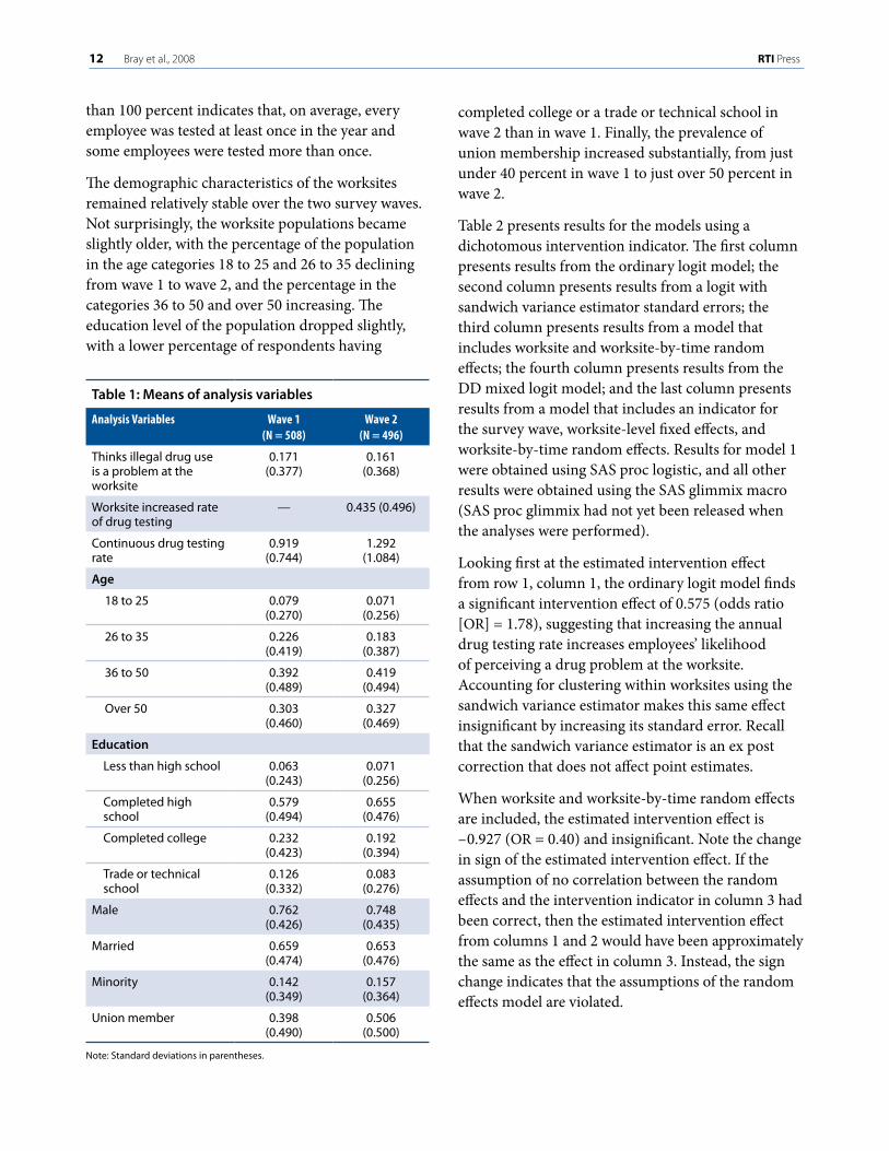
1� Bray et al., 2008 RTI Press

than 100 percent indicates that, on average, every employee was tested at least once in the year and some employees were tested more than once.

The demographic characteristics of the worksites remained relatively stable over the two survey waves. Not surprisingly, the worksite populations became slightly older, with the percentage of the population in the age categories 18 to 25 and 26 to 35 declining from wave 1 to wave 2, and the percentage in the categories 36 to 50 and over 50 increasing. The education level of the population dropped slightly, with a lower percentage of respondents having

completed college or a trade or technical school in wave 2 than in wave 1. Finally, the prevalence of union membership increased substantially, from just under 40 percent in wave 1 to just over 50 percent in wave 2.

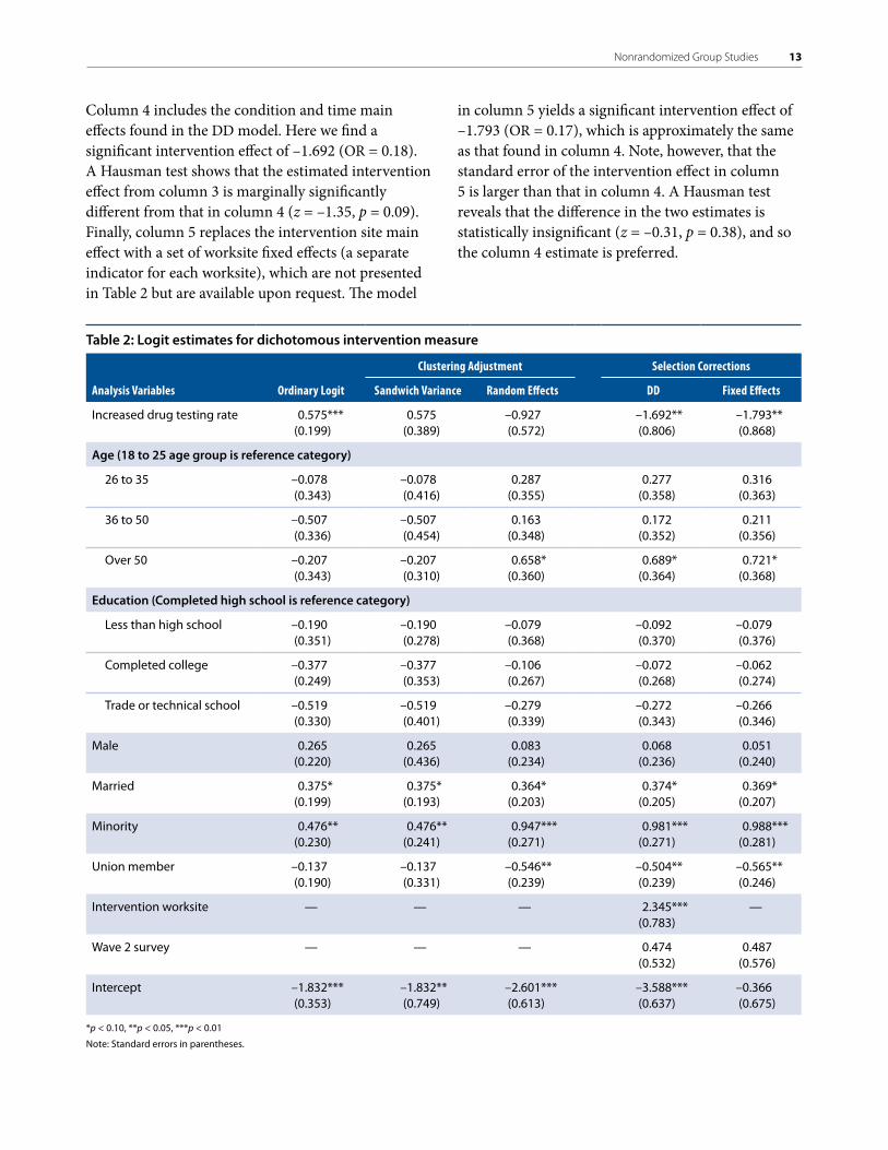
Table 2 presents results for the models using a dichotomous intervention indicator. The first column presents results from the ordinary logit model; the second column presents results from a logit with sandwich variance estimator standard errors; the third column presents results from a model that includes worksite and worksite-by-time random effects; the fourth column presents results from the DD mixed logit model; and the last column presents results from a model that includes an indicator for the survey wave, worksite-level fixed effects, and worksite-by-time random effects. Results for model 1 were obtained using SAS proc logistic, and all other results were obtained using the SAS glimmix macro (SAS proc glimmix had not yet been released when the analyses were performed).

Looking first at the estimated intervention effect from row 1, column 1, the ordinary logit model finds a significant intervention effect of 0.575 (odds ratio [OR] = 1.78), suggesting that increasing the annual drug testing rate increases employees’ likelihood of perceiving a drug problem at the worksite. Accounting for clustering within worksites using the sandwich variance estimator makes this same effect insignificant by increasing its standard error. Recall that the sandwich variance estimator is an ex post correction that does not affect point estimates.

When worksite and worksite-by-time random effects are included, the estimated intervention effect is – 0.927 (OR = 0.40) and insignificant. Note the change in sign of the estimated intervention effect. If the assumption of no correlation between the random effects and the intervention indicator in column 3 had been correct, then the estimated intervention effect from columns 1 and 2 would have been approximately the same as the effect in column 3. Instead, the sign change indicates that the assumptions of the random effects model are violated.

Table 1: Means of analysis variables

AnalysisVariables Wave1(N=508)

Wave2(N=496)

Thinks illegal drug use is a problem at the worksite

0.171 (0.377)

0.161 (0.368)

Worksite increased rate of drug testing

— 0.435 (0.496)

Continuous drug testing rate

0.919 (0.744)

1.292 (1.084)

Age

18 to 25 0.079 (0.270)

0.071 (0.256)

26 to 35 0.226 (0.419)

0.183 (0.387)

36 to 50 0.392 (0.489)

0.419 (0.494)

Over 50 0.303 (0.460)

0.327 (0.469)

Education

Less than high school 0.063 (0.243)

0.071 (0.256)

Completed high school

0.579 (0.494)

0.655 (0.476)

Completed college 0.232 (0.423)

0.192 (0.394)

Trade or technical school

0.126 (0.332)

0.083 (0.276)

Male 0.762 (0.426)

0.748 (0.435)

Married 0.659 (0.474)

0.653 (0.476)

Minority 0.142 (0.349)

0.157 (0.364)

Union member 0.398 (0.490)

0.506 (0.500)

Note: Standard deviations in parentheses.

Nonrandomized Group Studies 1�

Table 2: Logit estimates for dichotomous intervention measure

ClusteringAdjustment SelectionCorrections

AnalysisVariables OrdinaryLogit SandwichVariance RandomEffects DD FixedEffects

Increased drug testing rate 0.575***(0.199)

0.575(0.389)

–0.927(0.572)

–1.692**(0.806)

–1.793**(0.868)

Age (18 to 25 age group is reference category)

26 to 35 –0.078(0.343)

–0.078(0.416)

0.287(0.355)

0.277(0.358)

0.316(0.363)

36 to 50 –0.507(0.336)

–0.507(0.454)

0.163(0.348)

0.172(0.352)

0.211(0.356)

Over 50 –0.207(0.343)

–0.207(0.310)

0.658*(0.360)

0.689*(0.364)

0.721*(0.368)

Education (Completed high school is reference category)

Less than high school –0.190(0.351)

–0.190(0.278)

–0.079(0.368)

–0.092(0.370)

–0.079(0.376)

Completed college –0.377 (0.249)

–0.377(0.353)

–0.106(0.267)

–0.072(0.268)

–0.062(0.274)

Trade or technical school –0.519(0.330)

–0.519(0.401)

–0.279(0.339)

–0.272(0.343)

–0.266(0.346)

Male 0.265(0.220)

0.265(0.436)

0.083(0.234)

0.068(0.236)

0.051(0.240)

Married 0.375*(0.199)

0.375*(0.193)

0.364*(0.203)

0.374*(0.205)

0.369*(0.207)

Minority 0.476**(0.230)

0.476**(0.241)

0.947***(0.271)

0.981***(0.271)

0.988***(0.281)

Union member –0.137(0.190)

–0.137(0.331)

–0.546**(0.239)

–0.504**(0.239)

–0.565**(0.246)

Intervention worksite — — — 2.345***(0.783)

—

Wave 2 survey — — — 0.474(0.532)

0.487(0.576)

Intercept –1.832***(0.353)

–1.832**(0.749)

–2.601***(0.613)

–3.588***(0.637)

–0.366(0.675)

*p < 0.10, **p < 0.05, ***p < 0.01

Note: Standard errors in parentheses.

Column 4 includes the condition and time main effects found in the DD model. Here we find a significant intervention effect of –1.692 (OR = 0.18). A Hausman test shows that the estimated intervention effect from column 3 is marginally significantly different from that in column 4 (z = –1.35, p = 0.09). Finally, column 5 replaces the intervention site main effect with a set of worksite fixed effects (a separate indicator for each worksite), which are not presented in Table 2 but are available upon request. The model

in column 5 yields a significant intervention effect of –1.793 (OR = 0.17), which is approximately the same as that found in column 4. Note, however, that the standard error of the intervention effect in column 5 is larger than that in column 4. A Hausman test reveals that the difference in the two estimates is statistically insignificant (z = –0.31, p = 0.38), and so the column 4 estimate is preferred.

1� Bray et al., 2008 RTI Press

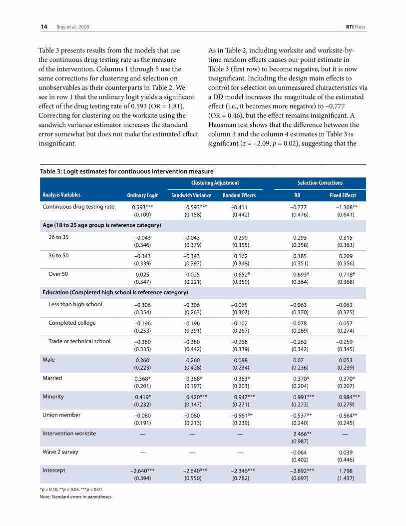
Table 3 presents results from the models that use the continuous drug testing rate as the measure of the intervention. Columns 1 through 5 use the same corrections for clustering and selection on unobservables as their counterparts in Table 2. We see in row 1 that the ordinary logit yields a significant effect of the drug testing rate of 0.593 (OR = 1.81). Correcting for clustering on the worksite using the sandwich variance estimator increases the standard error somewhat but does not make the estimated effect insignificant.

As in Table 2, including worksite and worksite-by-time random effects causes our point estimate in Table 3 (first row) to become negative, but it is now insignificant. Including the design main effects to control for selection on unmeasured characteristics via a DD model increases the magnitude of the estimated effect (i.e., it becomes more negative) to –0.777 (OR = 0.46), but the effect remains insignificant. A Hausman test shows that the difference between the column 3 and the column 4 estimates in Table 3 is significant (z = –2.09, p = 0.02), suggesting that the

Table 3: Logit estimates for continuous intervention measure

ClusteringAdjustment SelectionCorrections

AnalysisVariables OrdinaryLogit SandwichVariance RandomEffects DD FixedEffects

Continuous drug testing rate 0.593*** (0.100)

0.593*** (0.158)

–0.411 (0.442)

–0.777(0.476)

–1.308**(0.641)

Age (18 to 25 age group is reference category)

26 to 35 –0.043(0.346)

–0.043 (0.379)

0.290(0.355)

0.293(0.358)

0.315(0.363)

36 to 50 –0.343(0.339)

–0.343(0.397)

0.162(0.348)

0.185(0.351)

0.209(0.356)

Over 50 0.025(0.347)

0.025(0.221)

0.652*(0.359)

0.693*(0.364)

0.718* (0.368)

Education (Completed high school is reference category)

Less than high school –0.306(0.354)

–0.306(0.263)

–0.065(0.367)

–0.063(0.370)

–0.062(0.375)

Completed college –0.196(0.253)

–0.196(0.391)

–0.102(0.267)

–0.078(0.269)

–0.057(0.274)

Trade or technical school –0.380(0.335)

–0.380 (0.442)

–0.268 (0.339)

–0.262(0.342)

–0.259(0.345)

Male 0.260(0.223)

0.260 (0.428)

0.088(0.234)

0.07 (0.236)

0.053(0.239)

Married 0.368*(0.201)

0.368* (0.197)

0.363*(0.203)

0.370*(0.204)

0.370*(0.207)

Minority 0.419*(0.232)

0.420***(0.147)

0.947*** (0.271)

0.991*** (0.273)

0.984*** (0.279)

Union member –0.080(0.191)

–0.080 (0.213)

–0.561**(0.239)

–0.537**(0.240)

–0.564** (0.245)

Intervention worksite — — — 2.466** (0.987)

—

Wave 2 survey — — — –0.064 (0.402)

0.039(0.446)

Intercept –2.640***(0.394)

–2.640***(0.550)

–2.346***(0.782)

–2.892***(0.697)

1.798(1.437)

*p < 0.10, **p < 0.05, ***p < 0.01

Note: Standard errors in parentheses.

Nonrandomized Group Studies 1�

column 4 estimate is preferred over the column 3 estimate. Including worksite-level fixed effects, as in column 5, however, causes the estimated effect to become significant at –1.308 (OR = 0.27). As in Table 2, estimates for the worksite-level fixed effects are not presented but are available upon request.

A Hausman test shows that the difference between the column 4 and column 5 estimates is insignificant at the 0.10 level but significant at the 0.15 level (z = –1.23, p = 0.11). Although not a definitive rejection of the column 4 estimate, the low power of the Hausman test and the relatively substantial change in the magnitude of the estimated effect suggest that the column 5 estimates should be considered when making inferences about the estimated intervention effect.

DiscussionThe demand for the study of interventions that are implemented in real-world settings has resulted in more nonrandomized group studies’ being performed. A nonrandomized group study is a quasi-experimental study in which identifiable groups of individuals are assigned to the intervention and comparison groups in a systematic way. These designs have two major analysis challenges: clustered data and potential selection bias. Previous literature has identified a variety of methods for dealing with clustered data, including ex post corrections to the estimated variances, random effects models, and fixed effects models.

Several options are also available to correct for sample selection bias. If the selection is on measured characteristics, then researchers can simply include measures of the observed characteristics in their analyses. If selection is on unmeasured characteristics, then researchers need more complicated corrections, such as the Heckman model or IV techniques that estimate the selection process, or DD or fixed effects methods that do not estimate the selection process. Unfortunately, previous literature provides little guidance about analysis methods for researchers analyzing data from nonrandomized group studies.

We examined various methods for analyzing data from nonrandomized group studies. Many of the standard methods for addressing clustered data can be readily applied to nonrandomized group studies. Similarly, many of the methods for correcting for selection on unobserved characteristics can also be applied to nonrandomized group trial data. Techniques that estimate the selection process, however, require a sufficient number of groups (typically greater than 30) to model the group-level decision to participate in the intervention. Because many nonrandomized group trials have relatively few groups, these approaches may not be appropriate in many cases. Techniques that do not estimate the selection process, however, can be used whenever the researcher has access to both pre- and post-treatment data.

We used data from SAMHSA’s WMC Program to explore the estimated intervention effect using various estimation methods. We found that both clustering and sample selection corrections have substantial impacts on quantitative and qualitative conclusions about the effects of an intervention. In particular, we found that the estimated intervention effect can switch from positive and significant to negative and significant when both clustering and sample selection are addressed.

Based on these analyses, we propose the following recommendations to researchers analyzing nonrandomized group trial data. First, use random effects to account for all levels of identifiable clustering. Second, estimate DD models with random effects to account for clustering, and compare the results with those from the simple random effects model using a Hausman test. If the DD model does not yield significantly different estimates, then the simple random effects model is preferred. If the DD model does yield significantly different results, then it is preferred.

Finally, estimate a group-level fixed effects model (controlling for clustering at any level other than the group with random effects) and compare the results with the DD results using a Hausman test. If the fixed effects model does not yield significantly different estimates from the DD model, then the DD model is preferred. Otherwise, the fixed effects model is preferred.

1� Bray et al., 2008 RTI Press

Based on our empirical results, group-level fixed effects appear to be especially important in the presence of a continuous measure of the intervention, such as a continuous dose variable. For both continuous and discrete outcomes, all our proposed analyses can be easily performed in standard statistical software packages, such as SAS (using proc mixed or proc glimmix) or Stata (using xtmixed).

Although the methods proposed here will greatly improve researchers’ ability to draw inferences from nonrandomized group trial data, as with any

quasi-experimental design a causal interpretation must ultimately depend on the validity of the underlying theory or logic model that links the intervention to the outcome. No empirical strategy can alleviate concerns about the plausibility of an estimated intervention effect that arise from doubts about the underlying theory. However, strong empirical methods can help to eliminate competing explanations for the reasons an effect might be found. Thus, such methods can bolster theoretical arguments about the causal nature of any such intervention effect.

References

Farquhar, J. W., Fortmann, S. P., Flora, J. A., Taylor, B., Haskell, W. L., Williams, P. T., Maccoby, N., & Wood, P. D. (1990). Effects of communitywide education on cardiovascular disease risk factors: The Stanford Five-City Project. Journal of the American Medical Association, 264(3), 359–365.

Goldstein, H. (1987). Multilevel covariance component models. Biometrika, 74(2), 430–431.

Greene, W. H. (1997). Econometric analysis, third edition. New Jersey: Prentice-Hall.

Hausman, J. A. (1978). Specification tests in econometrics. Econometrica, 46(6), 1251–1271.

Heckman, J. (1979). Sample selection bias as a specification error. Econometrica, 47, 153–161.

Heckman, J. (1997). Instrumental variables: A study of implicit behavioral assumptions used in making program evaluations. The Journal of Human Resources, 32(3), 441–462.

Heckman J. J., & Hotz, V. J. (1989). Choosing among alternative nonexperimental methods for estimating the impact of social programs: The case of manpower training. Journal of the American Statistical Association, 84(408), 862–880.

Heckman, J. J., & Robb, R. (1985). Alternative methods for evaluating the impact of interventions: An overview. Journal of Economics, 30, 239–267.

Hsiao, C. (1986). Analysis of panel data. Cambridge, MA: Cambridge University Press.

Ames, G. M., Grube, J. W., & Moore, R. S. (2000). Social control and workplace drinking norms: A comparison of two organizational cultures. Journal of Studies on Alcohol, 61, 203–219.

Baltagi, B. H. (1995). Econometric analysis of panel data. Chichester (UK): John Wiley & Sons.

Barnow, B. S., Cain, G. G., & Goldberger, A. S. (1980). Issues in the analysis of selectivity bias. In E. Stromsdorfer & G. Farkas (Eds.), Evaluation studies, Vol. 5. San Francisco: Sage.

Blank, D., Walsh, J. M., & Cangianelli, L. (2002). Effect of drug-testing and prevention education strategies on employee behavior and attitudes at a manufacturing company. Working paper. Bethesda, MD: The Walsh Group, P.A.

Bryk, A. S., & Raudenbush, S. W. (1988). Toward a more appropriate conceptualization of research on school effects: A three-level hierarchical linear model. American Journal of Education, 97(1), 65–108.

Carleton, R. A., Lasater, T. M., Assaf, A. R., Feldman, H. A., McKinlay, S., & the Pawtucket Heart Health Program Writing Group (1995). The Pawtucket Heart Health Program: Community changes in cardiovascular risk factors and projected disease risk. American Journal of Public Health, 85(6), 777–785.

Cook, T. D., & Campbell, D. T. (1979). Quasi-experimentation: Design and analysis issues for field settings. Boston: Houghton Mifflin Company.

Nonrandomized Group Studies 1�

Huber, P. J. (1967). The behavior of maximum likelihood estimates under nonstandard conditions. In Proceedings of the fifth Berkeley Symposium on Mathematical Statistics and Probability, 1, 221–233.

Ichimura, H. & Taber, C. (2001). Propensity-score matching with instrumental variables. American Economic Review, 91(2), 119-124.

Lapham, S. C., Chang, I., & Gregory, C. (2000). Substance abuse intervention for health care workers: A preliminary report. Journal of Behavioral Health Services Research, 27, 131–143.

Liang, K. Y., & Zeger, S. L. (1986). Longitudinal data analysis using generalized linear models. Biometrika, 73, 13–22.

Luepker, R. V. (1994). Community trials. Preventive Medicine, 23, 602–605.

Murray, D. M. (1997). Design and analysis of group-randomized trials: A review of recent developments. Annals of Epidemiology, 7(57), S69 S77.

Murray, D. M. (1998). Design and analysis of group randomized trials. New York: Oxford University Press.

Murray, D. M., Hannan, P. J., & Baker, W. L. (1996). A Monte Carlo study of alternative responses to intraclass correlation in community trials: Is it ever possible to avoid Cornfield’s penalties? Evaluation Review, 20(3), 313–337.

Newhouse, J. P., & McClellan, M. (1998). Econometrics in outcomes research: The use of instrumental variables. Annual Review of Public Health, 19, 17–34.

Norton, E. C., Bieler, G. S., Ennett, S. T., & Zarkin, G. A. (1996). Analysis of prevention program effectiveness with clustered data using generalized estimating equations. Journal of Consulting and Clinical Psychology, 64(5), 919–926.

Reichardt, C. S. (1979). The statistical analysis of data from nonequivalent group designs. In T.D. Cook & D.T. Campbell (Eds.) Quasi-experimentation: Design & analysis issues for field settings. Boston: Houghton Mifflin Company, 147–205.

Rosenbaum, P. R., & Rubin, D. B. (1984). Reducing bias in observational studies using subclassification on the propensity score. Journal of the American Statistical Association, 79, 516–524.

SAS Institute Inc. (2002–2004). SAS 9.1.3 Help and Documentation. Cary, NC: Author.

StataCorp (2005). Stata Statistical Software: Release 9. College Station, TX: Author.

White, H. (1980). A heteroskedasticity-consistent covariance matrix and a direct test for heteroskedasticity. Econometrica, 48, 817–838.

Williams, R. L. (2000). A note on robust variance estimation for cluster-correlated data. Biometrics, 56(2), 645-646.

Zarkin, G. A., Bray, J. W., Karuntzos, G. T., & Demiralp, B. (2001). The effect of an enhanced employee assistance program (EAP) intervention on EAP utilization. Journal of Studies on Alcohol, 62(3), 351–358.

Zucker, D. M. (1990). An analysis of variance pitfall: The fixed effects analysis in a nested design. Educational Psychology Measures, 50, 731–738.

AcknowledgmentsFunding for this work was provided by the Office of Workplace Programs, Center for Substance Abuse Prevention through a subcontract with the CDM Group. The authors would like to thank the Workplace Managed Care Steering Committee and Publications Subcommittee for helpful suggestions. The authors also thank Susan Murchie, MA, for editorial assistance and Erica Brody, MPH, and Christian Evensen, MS, for research assistance. The opinions expressed are not necessarily those of RTI International or the Center for Substance Abuse Prevention, Substance Abuse and Mental Health Services Administration.

RTI International is an independent, nonprofit research organization dedicated to improving the human condition by turning knowledge into practice. RTI offers innovative research and technical solutions to governments and businesses worldwide in the areas of health and pharmaceuticals, education and training, surveys and statistics, advanced technology, international development, economic and social policy, energy, and the environment.

The RTI Press complements traditional publication outlets by providing another way for RTI researchers to disseminate the knowledge they generate. This PDF document is offered as a public service of RTI International. More information about RTI Press can be found at www.rti.org/rtipress.

www.rti.org/rtipress RTI Press publication MR-000�-0�11