Embed Size (px)
Citation preview

Analyzing the Spectrum of Asset Returns: Jumpand Volatility Components in High Frequency Data
Yacine A��t-Sahalia Jean JacodPrinceton University Universit�e de Paris VI
1
1 INTRODUCTION
1. Introduction
� Basic framework: X, often the log of an asset price, is assumed tofollow an Ito semimartingale.
� A semimartingale can be decomposed into the sum of a drift, a con-
tinuous Brownian-driven part and a discontinuous, or jump, part.
{ The jump part can in turn be decomposed into a sum of small
jumps and big jumps.
{ Such a process will always generate a �nite number of big jumps.
{ But it may give rise to either a �nite or in�nite number of small
jumps.
2
1 INTRODUCTION
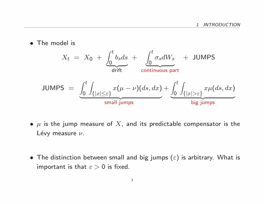
� The model is
Xt = X0 +Z t0bsds| {z }drift
+Z t0�sdWs| {z }
continuous part
+ JUMPS
JUMPS =Z t0
Zfjxj�"g
x(�� �)(ds; dx)| {z }small jumps
+Z t0
Zfjxj>"g
x�(ds; dx)| {z }big jumps
� � is the jump measure of X, and its predictable compensator is theL�evy measure �.
� The distinction between small and big jumps (") is arbitrary. What isimportant is that " > 0 is �xed.
3
1 INTRODUCTION
� In earlier work, we developed tests to determine on the basis of theobserved sampled path on [0; T ]:
{ whether a jump part was present
{ whether the jumps had �nite or in�nite activity
{ in the latter situation proposed a de�nition and an estimator of a
degree of jump activity parameter
{ whether a Brownian continuous component was needed once in�-
nite activity jumps are included
� In this talk, we show how these di�erent results can be put in a com-mon framework using a common methodology.
4
1 INTRODUCTION
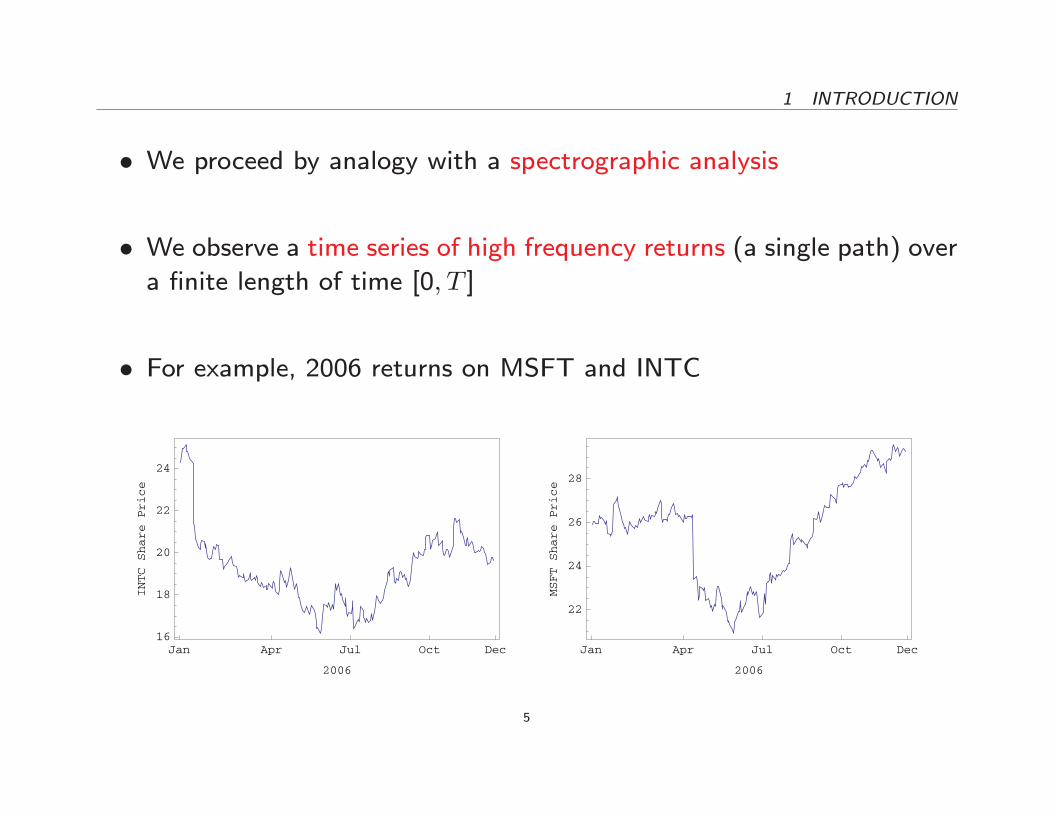
� We proceed by analogy with a spectrographic analysis
� We observe a time series of high frequency returns (a single path) overa �nite length of time [0; T ]
� For example, 2006 returns on MSFT and INTC
Jan Apr Jul Oct Dec16
18
20
22
24
2006
INTCSharePrice
Jan Apr Jul Oct Dec
22
24
26
28
2006
MSFTSharePrice
5

1 INTRODUCTION
� And then design a set of statistical tools that can tell us somethingabout speci�c components of the process that produced the observa-
tions
� These tools play the role of the measurement devices used in astro-physics to analyze the light emanating from a star, for instance
{ our observations are the high frequency returns; in astrophysics it's
the light (visible or not)
{ here the data generating mechanism is assumed to be a semimartin-
gale; in astrophysics it's whatever nuclear reactions inside the star
are producing the light
6

1 INTRODUCTION
� In astrophysics, one can look at a speci�c range of the light spectrumto learn something about speci�c chemical elements present in the star
� Here, we design statistics that focus on speci�c parts of the distri-bution of high frequency returns in order to learn something about
the di�erent components of the semimartingale that produced those
returns
{ decide which component(s) need to be included in the model (jumps,�nite or in�nite activity, continuous component, etc.)
{ determine their relative magnitude
{ magnify speci�c components of the model if they are present, sowe can analyze their �ner characteristics (such as the degree of
activity of jumps)
7
1 INTRODUCTION
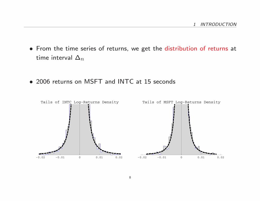
� From the time series of returns, we get the distribution of returns at
time interval �n
� 2006 returns on MSFT and INTC at 15 seconds
-0.02 -0.01 0 0.01 0.02
Tails of INTC Log-Returns Density
-0.02 -0.01 0 0.01 0.02
Tails of MSFT Log-Returns Density
8
1 INTRODUCTION
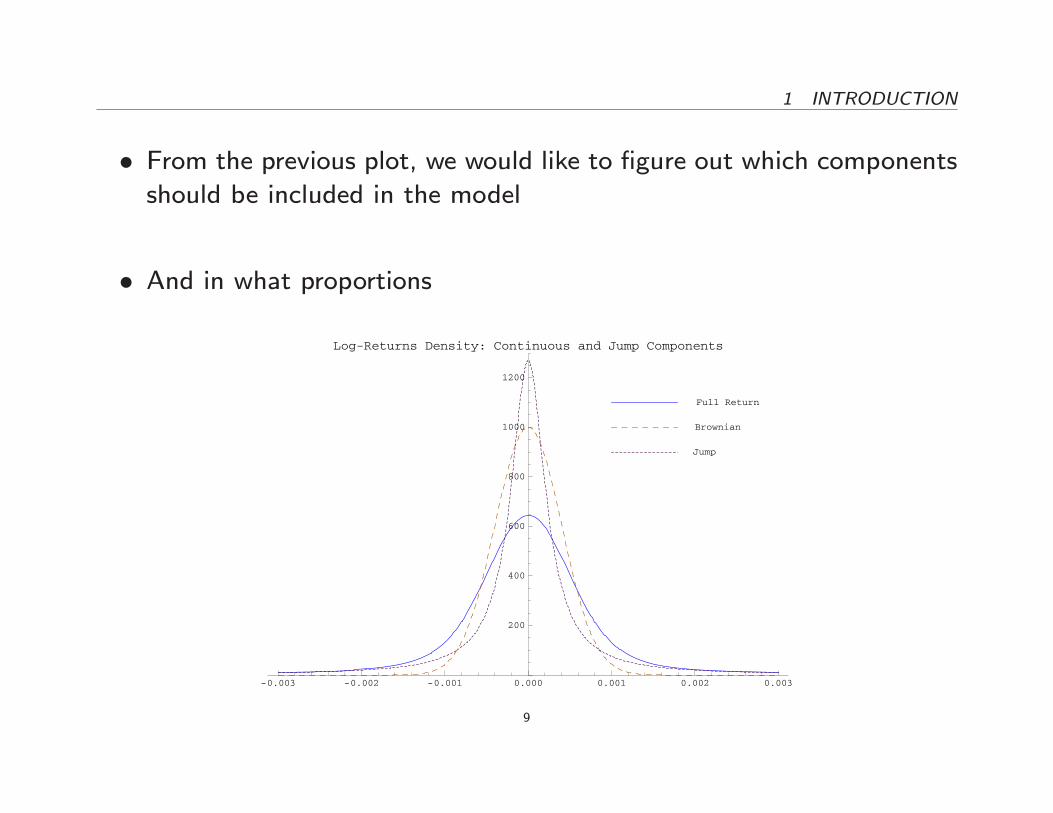
� From the previous plot, we would like to �gure out which components
should be included in the model
� And in what proportions
-0.003 -0.002 -0.001 0.000 0.001 0.002 0.003
200
400
600
800
1000
1200
Log-Returns Density: Continuous and Jump Components
Full Return
Brownian
Jump
9

1 INTRODUCTION
� Similarly to what is done in spectrographic analysis
{ we will emphasize visual tools
{ so we will only include the LLN here
{ and refer to the underlying papers for the formal derivations in-
cluding regularity conditions and the CLT, as well as simulations.
10
2 THE MEASUREMENT DEVICE
2. The Measurement Device
� We construct power variations of the increments, suitably truncatedand/or sampled at di�erent frequencies.
� We exploit the di�erent asymptotic behavior of the variations as wevary:
{ the power p
{ the truncation level u
{ the sampling frequency �
11
2 THE MEASUREMENT DEVICE
� This gives us three degrees of freedom, or tuning parameters, withenough exibility to isolate what we are looking for.
� Having these three parameters to play with, p; u and �; is like havingthree knobs to adjust in the measurement device.
12

2 THE MEASUREMENT DEVICE
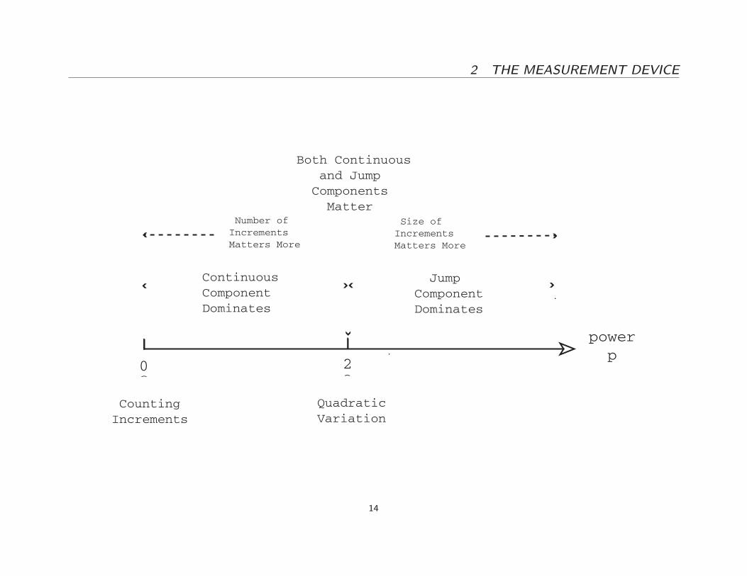
� Varying the power
{ Powers p < 2 will emphasize the continuous component of the
underlying sampled process.
{ Powers p > 2 will conversely accentuate its jump component.
{ The power p = 2 puts them on an equal footing.
13
2 THE MEASUREMENT DEVICE
power p
0 2
CountingIncrements
QuadraticVariation
ContinuousComponentDominates
JumpComponentDominates
Number ofIncrementsMatters More
Size ofIncrementsMatters More
Both Continuous and Jump Components Matter
14
2 THE MEASUREMENT DEVICE
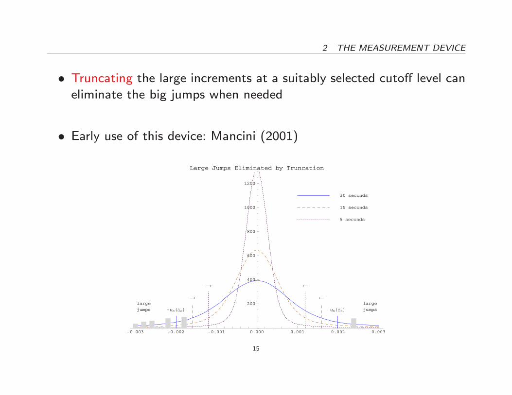
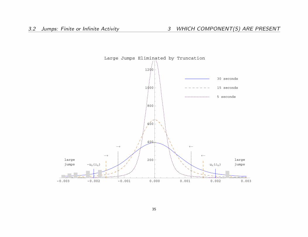
� Truncating the large increments at a suitably selected cuto� level caneliminate the big jumps when needed
� Early use of this device: Mancini (2001)
-0.003 -0.002 -0.001 0.000 0.001 0.002 0.003
200
400
600
800
1000
1200
Large Jumps Eliminated by Truncation
-un(Δn) un(Δn)
large
jumps
large
jumps
30 seconds
15 seconds
5 seconds
15
2 THE MEASUREMENT DEVICE
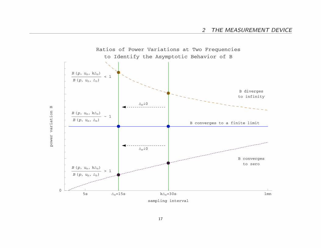
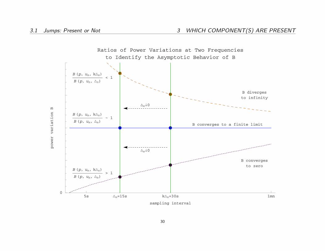
� Sampling at di�erent frequencies can let us distinguish between situ-ations where the variations:
{ converge to a �nite limit;
{ converge to zero;
{ diverge to in�nity.
16
2 THE MEASUREMENT DEVICE
5s Δn=15s kΔn=30s 1mn0
sampling interval
powervariationB
Ratios of Power Variations at Two Frequencies
to Identify the Asymptotic Behavior of B
B diverges
to infinity
B converges to a finite limit
B converges
to zero
B (p, un, kΔn)
B (p, un, Δn)~ 1
B (p, un, kΔn)
B (p, un, Δn)< 1
B (p, un, kΔn)
B (p, un, Δn)> 1
Δn↓0
Δn↓0
17
2 THE MEASUREMENT DEVICE
� These various limiting behaviors of the variations are indicative ofwhich component of the model dominates at a particular power and
in a certain range of returns (by truncation)
� Just like certain chemical elements have a very speci�c spectrographicsignature.
� So they e�ectively allow us to distinguish between all manners of nulland alternative hypotheses.
18
2 THE MEASUREMENT DEVICE
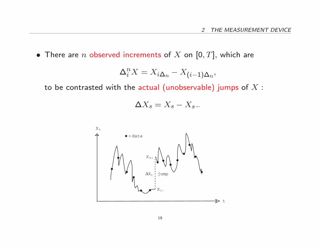
� There are n observed increments of X on [0; T ]; which are
�niX = Xi�n �X(i�1)�n;
to be contrasted with the actual (unobservable) jumps of X :
�Xs = Xs �Xs�
X
t
t
ΔXt
Xt-
Xt+
data=
jump
19
2 THE MEASUREMENT DEVICE
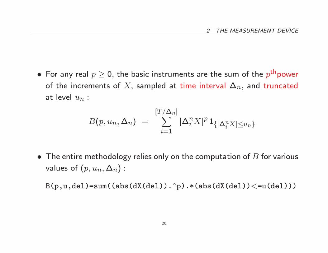
� For any real p � 0; the basic instruments are the sum of the pthpower
of the increments of X; sampled at time interval �n; and truncated
at level un :
B(p; un;�n) =[T=�n]Xi=1
j�niXjp 1fj�ni Xj�ung
� The entire methodology relies only on the computation of B for variousvalues of (p; un;�n) :
B(p,u,del)=sum((abs(dX(del)).^p).*(abs(dX(del))<=u(del)))
20
2 THE MEASUREMENT DEVICE
� T is �xed, asymptotics are all with respect to �n ! 0:
� un is the cuto� level for truncating the increments
� un ! 0 when n!1: in the form un = ��$n for some $ 2 (0; 1=2):
� $ < 1=2 to keep all the increments which contain a Brownian contri-
bution.
� There will be further restrictions on the rate at which un ! 0, ex-
pressed in the form of restrictions on the choice of $.
� If we don't want to truncate, we write B(p;1;�n):21
2 THE MEASUREMENT DEVICE
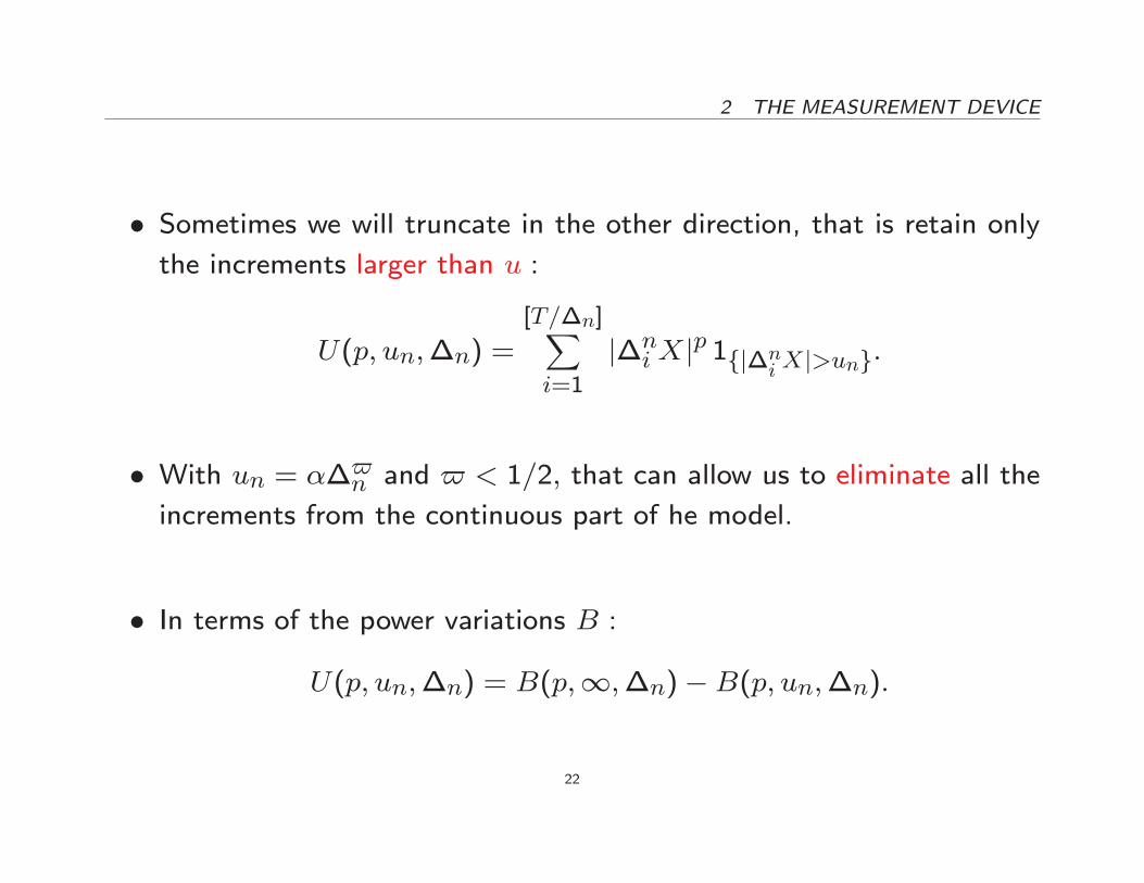
� Sometimes we will truncate in the other direction, that is retain onlythe increments larger than u :
U(p; un;�n) =[T=�n]Xi=1
j�niXjp 1fj�ni Xj>ung:
� With un = ��$n and $ < 1=2; that can allow us to eliminate all the
increments from the continuous part of he model.
� In terms of the power variations B :
U(p; un;�n) = B(p;1;�n)�B(p; un;�n):
22
2 THE MEASUREMENT DEVICE
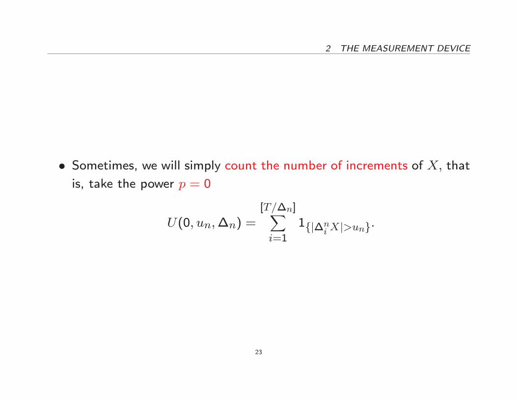
� Sometimes, we will simply count the number of increments of X; thatis, take the power p = 0
U(0; un;�n) =[T=�n]Xi=1
1fj�ni Xj>ung:
23
3 WHICH COMPONENT(S) ARE PRESENT
3. Which Component(s) Are Present
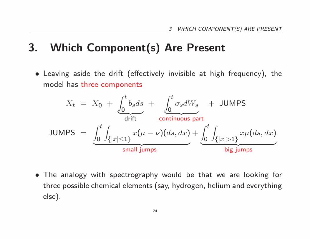
� Leaving aside the drift (e�ectively invisible at high frequency), themodel has three components
Xt = X0 +Z t0bsds| {z }drift
+Z t0�sdWs| {z }
continuous part
+ JUMPS
JUMPS =Z t0
Zfjxj�1g
x(�� �)(ds; dx)| {z }small jumps
+Z t0
Zfjxj>1g
x�(ds; dx)| {z }big jumps
� The analogy with spectrography would be that we are looking forthree possible chemical elements (say, hydrogen, helium and everything
else).
24
3 WHICH COMPONENT(S) ARE PRESENT
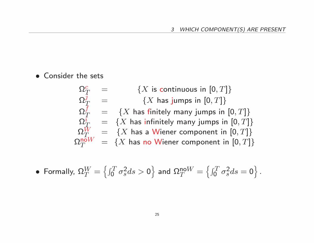
� Consider the setscT = fX is continuous in [0; T ]gjT = fX has jumps in [0; T ]g
fT = fX has finitely many jumps in [0; T ]g
iT = fX has in�nitely many jumps in [0; T ]gWT = fX has a Wiener component in [0; T ]gnoWT = fX has no Wiener component in [0; T ]g
� Formally, WT =nR T0 �
2sds > 0
oand noWT =
nR T0 �
2sds = 0
o:
25
3 WHICH COMPONENT(S) ARE PRESENT
� We observe a time series and wish to determine in which set(s) thepath was.
� There are theoretically many possible ways to do this, even if we re-strict attention to power variations only.
� However, we wish to construct test statistics that are model-free inthe sense that:
{ their implementation does not require that we estimate or calibratethe model, which can potentially be quite complicated (stochasticvolatility, jumps, jumps in volatility, jumps in jump intensity, etc.)
{ so we want the distribution of the test statistics to be assessedusing only power variations (of perhaps other powers, truncationlevels and sampling frequencies)
26
3.1 Jumps: Present or Not 3 WHICH COMPONENT(S) ARE PRESENT
3.1. Jumps: Present or Not
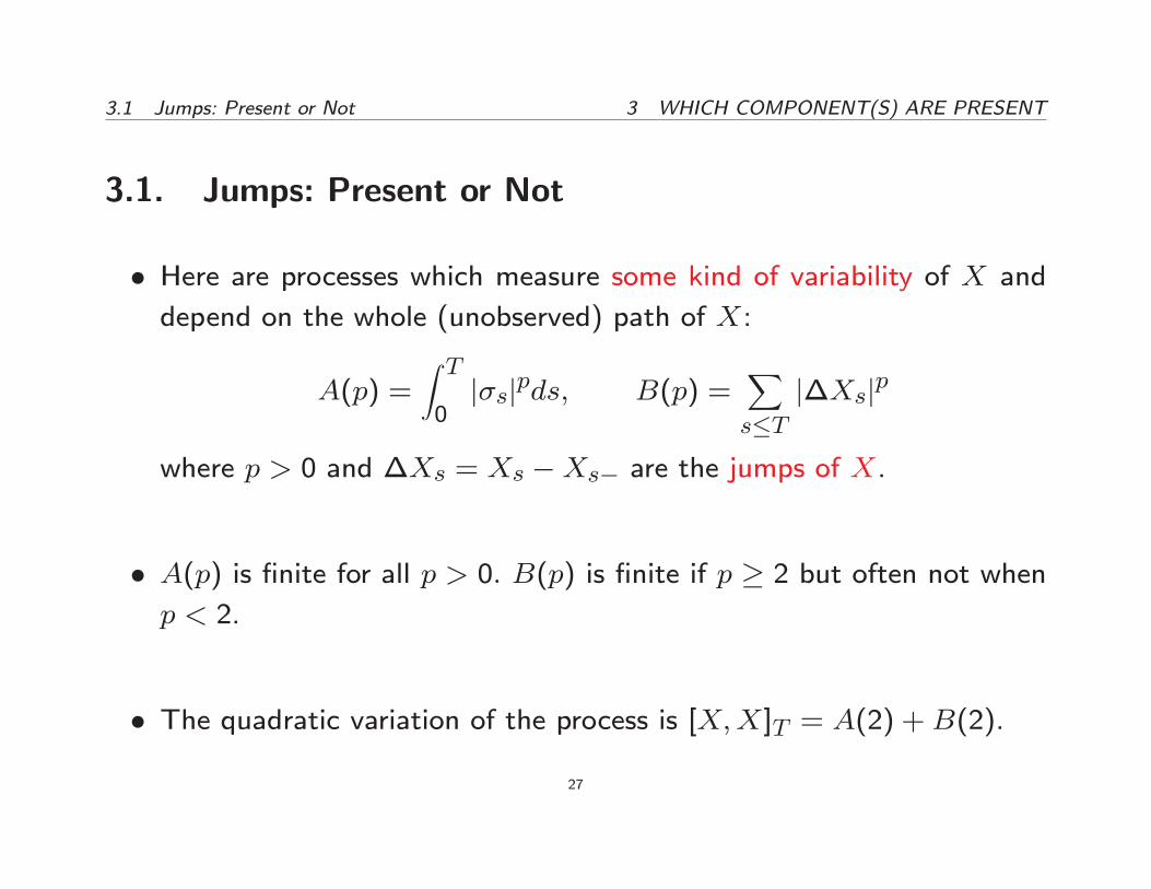
� Here are processes which measure some kind of variability of X and
depend on the whole (unobserved) path of X:
A(p) =Z T0j�sjpds; B(p) =
Xs�T
j�Xsjp
where p > 0 and �Xs = Xs �Xs� are the jumps of X.
� A(p) is �nite for all p > 0: B(p) is �nite if p � 2 but often not when
p < 2.
� The quadratic variation of the process is [X;X]T = A(2) +B(2).
27
3.1 Jumps: Present or Not 3 WHICH COMPONENT(S) ARE PRESENT
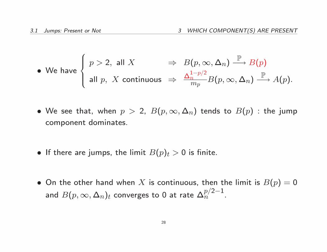
� We have
8>><>>:p > 2; all X ) B(p;1;�n) P�! B(p)
all p; X continuous ) �1�p=2nmp
B(p;1;�n) P�! A(p):
� We see that, when p > 2, B(p;1;�n) tends to B(p) : the jumpcomponent dominates.
� If there are jumps, the limit B(p)t > 0 is �nite.
� On the other hand when X is continuous, then the limit is B(p) = 0
and B(p;1;�n)t converges to 0 at rate �p=2�1n .
28
3.1 Jumps: Present or Not 3 WHICH COMPONENT(S) ARE PRESENT
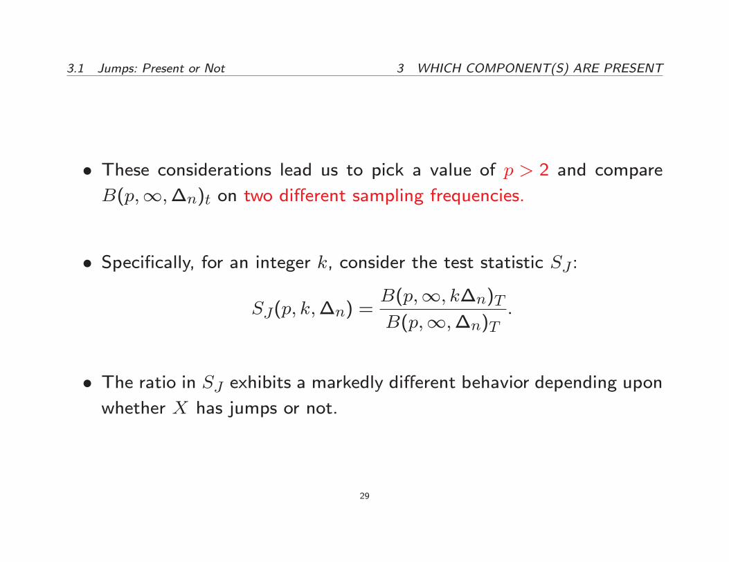
� These considerations lead us to pick a value of p > 2 and compareB(p;1;�n)t on two di�erent sampling frequencies.
� Speci�cally, for an integer k, consider the test statistic SJ :
SJ(p; k;�n) =B(p;1; k�n)TB(p;1;�n)T
:
� The ratio in SJ exhibits a markedly di�erent behavior depending uponwhether X has jumps or not.
29
3.1 Jumps: Present or Not 3 WHICH COMPONENT(S) ARE PRESENT
5s Δn=15s kΔn=30s 1mn0
sampling interval
powervariationB
Ratios of Power Variations at Two Frequencies
to Identify the Asymptotic Behavior of B
B diverges
to infinity
B converges to a finite limit
B converges
to zero
B (p, un, kΔn)
B (p, un, Δn)~ 1
B (p, un, kΔn)
B (p, un, Δn)< 1
B (p, un, kΔn)
B (p, un, Δn)> 1
Δn↓0
Δn↓0
30
3.1 Jumps: Present or Not 3 WHICH COMPONENT(S) ARE PRESENT
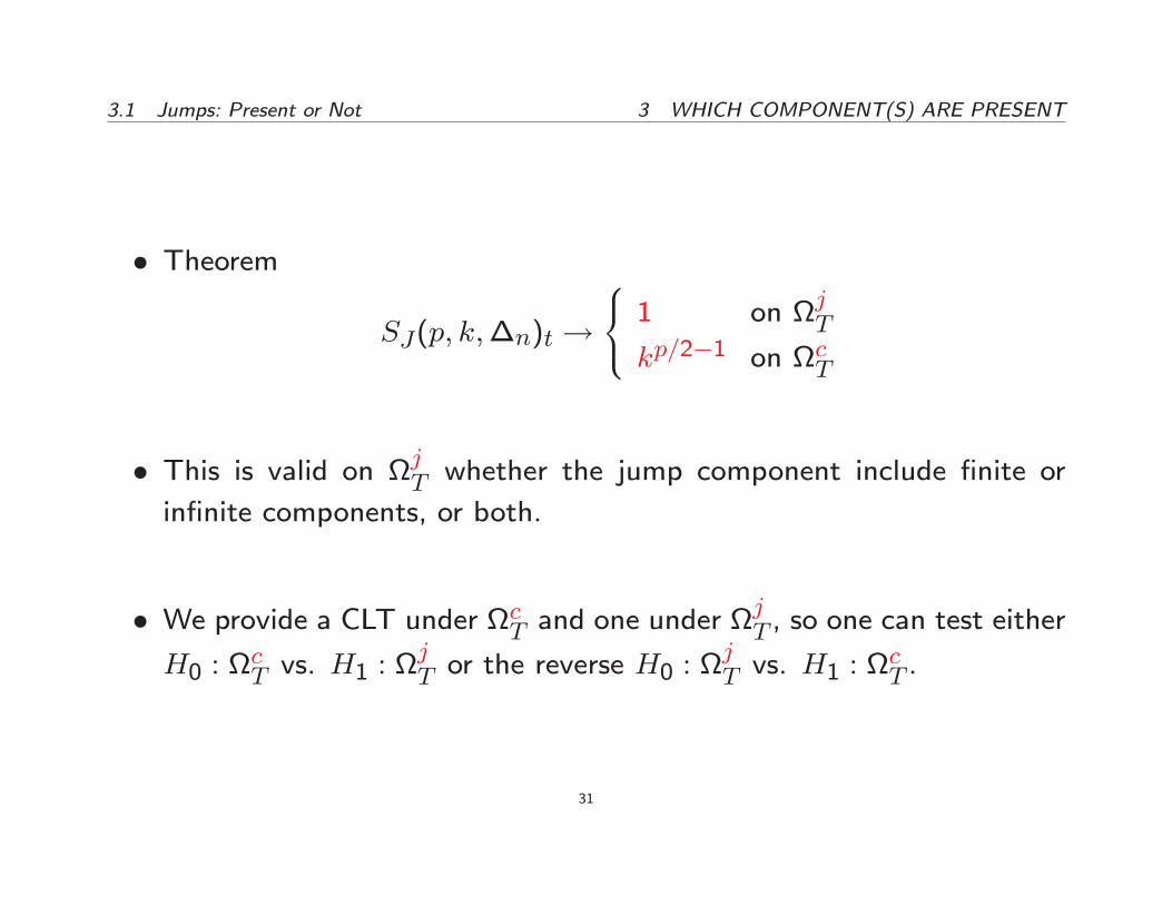
� Theorem
SJ(p; k;�n)t !
8<: 1 on jT
kp=2�1 on cT
� This is valid on jT whether the jump component include �nite or
in�nite components, or both.
� We provide a CLT under cT and one under jT , so one can test either
H0 : cT vs. H1 :
jT or the reverse H0 :
jT vs. H1 :
cT .
31
3.2 Jumps: Finite or In�nite Activity 3 WHICH COMPONENT(S) ARE PRESENT
3.2. Jumps: Finite or In�nite Activity
� Many models in mathematical �nance do not include jumps.
� But among those that do, the framework most often adopted consistsof a jump-di�usion: these models include a drift term, a Brownian-
driven continuous part, and a �nite activity jump part (compound Pois-
son process): early examples include Merton (1976), Ball and Torous
(1983) and Bates (1991).
� Other models are based onin�nite activity jumps: see for exampleMadan and Seneta (1990), Eberlein and Keller (1995), Barndor�-
Nielsen (1998), Carr, Geman, Madan and Yor (2002), Carr and Wu
(2003), etc.
32
3.2 Jumps: Finite or In�nite Activity 3 WHICH COMPONENT(S) ARE PRESENT
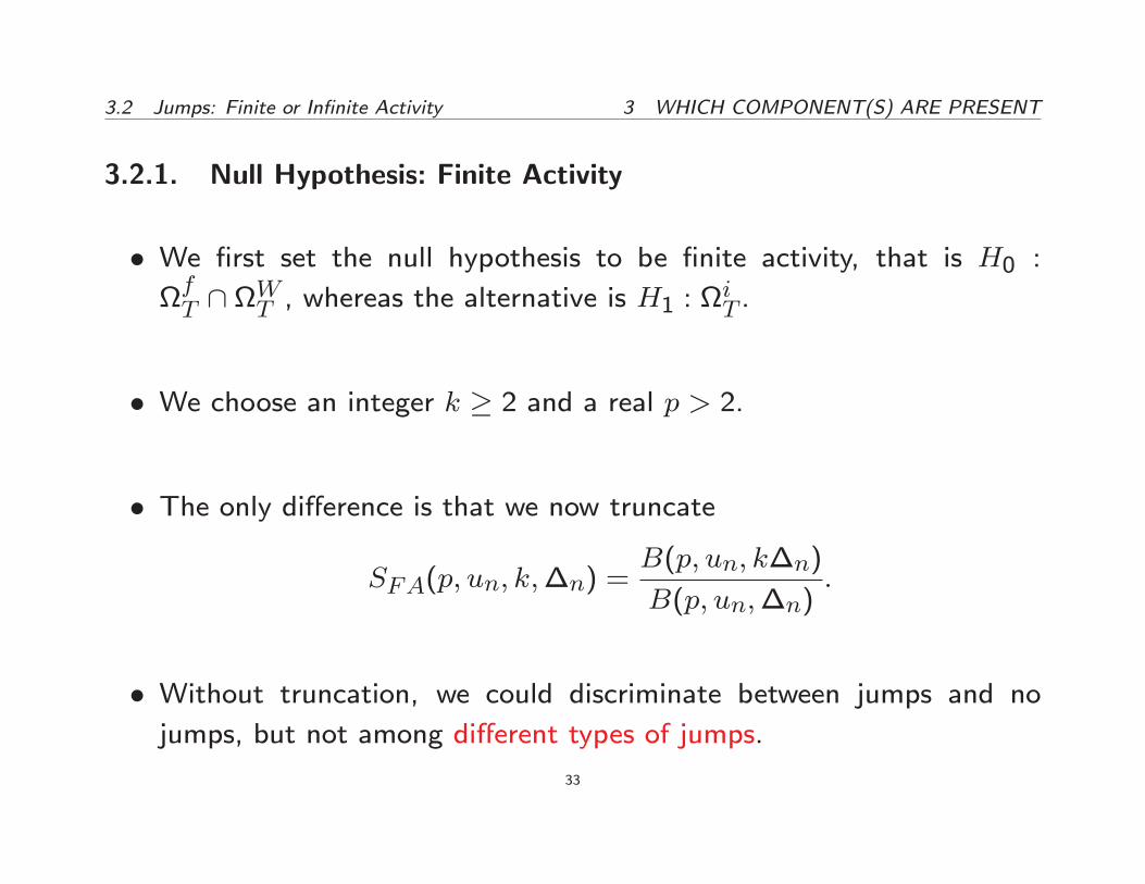
3.2.1. Null Hypothesis: Finite Activity
� We �rst set the null hypothesis to be �nite activity, that is H0 :fT \
WT , whereas the alternative is H1 :
iT .
� We choose an integer k � 2 and a real p > 2.
� The only di�erence is that we now truncate
SFA(p; un; k;�n) =B(p; un; k�n)
B(p; un;�n):
� Without truncation, we could discriminate between jumps and nojumps, but not among di�erent types of jumps.
33

3.2 Jumps: Finite or In�nite Activity 3 WHICH COMPONENT(S) ARE PRESENT
� Like before, we set p > 2 to magnify the jump component.
� But since we want to separate big and small jumps, we now truncateas a means of eliminating the large jumps.
� Since the large jumps are of �nite size (independent of �n), at somepoint in the asymptotics �n # 0; the truncation level un = O(�
�n)
will have eliminated all the large jumps.
34
3.2 Jumps: Finite or In�nite Activity 3 WHICH COMPONENT(S) ARE PRESENT
-0.003 -0.002 -0.001 0.000 0.001 0.002 0.003
200
400
600
800
1000
1200
Large Jumps Eliminated by Truncation
-un(Δn) un(Δn)
large
jumps
large
jumps
30 seconds
15 seconds
5 seconds
35

3.2 Jumps: Finite or In�nite Activity 3 WHICH COMPONENT(S) ARE PRESENT
� Then if there are only big jumps and the Brownian component, thetwo power variations B(p; un; k�n) and B(p; un;�n) will behave as
if there were no jumps and the limit of the ratio will be 2 as in the
test for jumps.
� But if there are small jumps, then the truncation cannot eliminate thembecause their size is �n�dependent then each B truncated tends to
the small of remaining jumps and the ratio tends to 1:
36
3.2 Jumps: Finite or In�nite Activity 3 WHICH COMPONENT(S) ARE PRESENT
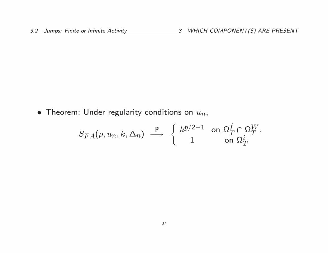
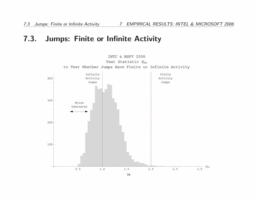
� Theorem: Under regularity conditions on un;
SFA(p; un; k;�n)P�!
(kp=2�1 on
fT \
WT :
1 on iT
37
3.2 Jumps: Finite or In�nite Activity 3 WHICH COMPONENT(S) ARE PRESENT
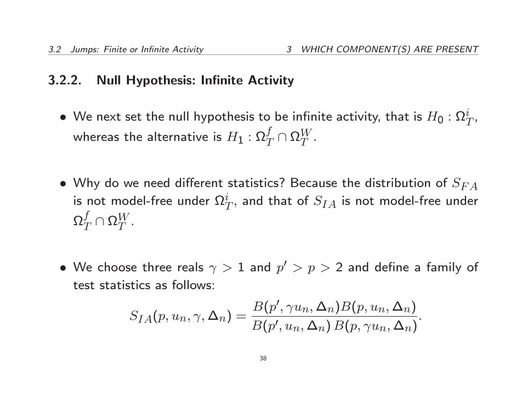
3.2.2. Null Hypothesis: In�nite Activity
� We next set the null hypothesis to be in�nite activity, that is H0 : iT ,whereas the alternative is H1 :
fT \
WT :
� Why do we need di�erent statistics? Because the distribution of SFAis not model-free under iT ; and that of SIA is not model-free under
fT \
WT :
� We choose three reals > 1 and p0 > p > 2 and de�ne a family of
test statistics as follows:
SIA(p; un; ;�n) =B(p0; un;�n)B(p; un;�n)B(p0; un;�n)B(p; un;�n)
:
38

3.2 Jumps: Finite or In�nite Activity 3 WHICH COMPONENT(S) ARE PRESENT
� Theorem: Under regularity conditions on un;
SIA(p; un; ;�n)P�!
( p
0�p on iT1 on
fT \
WT
39

3.3 Brownian Motion: Present or Not 3 WHICH COMPONENT(S) ARE PRESENT
3.3. Brownian Motion: Present or Not
� We would like to construct procedures which allow to:
{ decide whether the Brownian motion is really there
{ or if it can be forgone with in favor of a pure jump process with
in�nite activity.
� When in�nitely many jumps are included, there are a number of modelsin the literature which dispense with the Brownian motion altogether.
The log-price process is then a purely discontinuous L�evy process with
in�nite activity jumps, or more generally is driven by such a process:
see for example Madan and Seneta (1990), Eberlein and Keller (1995),
Carr, Geman, Madan and Yor (2002), Carr and Wu (2003), etc.
40

3.3 Brownian Motion: Present or Not 3 WHICH COMPONENT(S) ARE PRESENT
3.3.1. Null Hypothesis: Brownian Motion Present
� In order to construct a test, we seek a statistic with markedly di�erentbehavior under the null and alternative.
� The idea is now to consider powers less than 2
{ since in the presence of Brownian motion the power variation would
be dominated by it
{ while in its absence it would behave quite di�erently.
41
3.3 Brownian Motion: Present or Not 3 WHICH COMPONENT(S) ARE PRESENT
� Speci�cally, the large number of small increments generated by a con-tinuous component would cause a power variation of order less than
2 to diverge to in�nity.
� Without the Brownian motion, however, and when p > �, the power
variation converges to 0 at exactly the same rate for the two sampling
frequencies �n and k�n
� Whereas with a Brownian motion the choice of sampling frequencywill in uence the magnitude of the divergence.
� Taking a ratio will eliminate all unnecessary aspects of the problemand focus on that key aspect.
42
3.3 Brownian Motion: Present or Not 3 WHICH COMPONENT(S) ARE PRESENT
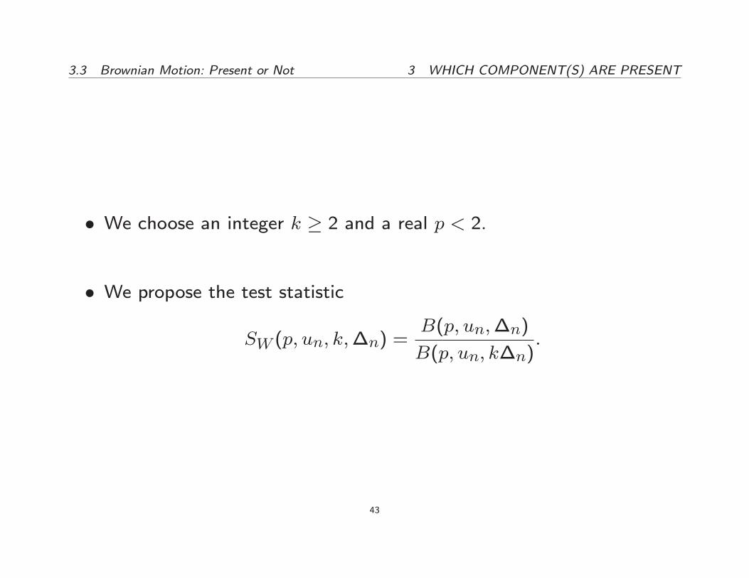
� We choose an integer k � 2 and a real p < 2.
� We propose the test statistic
SW (p; un; k;�n) =B(p; un;�n)
B(p; un; k�n):
43

3.3 Brownian Motion: Present or Not 3 WHICH COMPONENT(S) ARE PRESENT
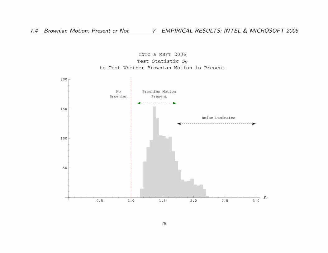
� Theorem: Under regularity conditions on un;
SW (p; un; k;�n)P�!
(k1�p=2 on WT1 on noWT \ iT ; p > �
44

3.3 Brownian Motion: Present or Not 3 WHICH COMPONENT(S) ARE PRESENT
� An alternative: Tauchen and Todorov (2009)
� They employ the test statistic for jumps SJ , plot its logarithm for
di�erent values of the power argument and contrast the behavior of
the plot above two and below two in order to identify the presence of
a Brownian component.
� This works when there is a Brownian motion is present under the null.
45
3.3 Brownian Motion: Present or Not 3 WHICH COMPONENT(S) ARE PRESENT
3.3.2. Null Hypothesis: No Brownian Motion
� The null model is now pure jump (plus perhaps a drift) with jumps.
{ When there are no jumps, or �nitely many jumps, and no Brownian
motion, X reduces to a pure drift plus occasional jumps, and such
a model is fairly unrealistic in the context of most �nancial data
series.
{ But one can certainly consider models that consist only of a jump
component, plus perhaps a drift, if that jump component is allowed
to be in�nitely active.
46
3.3 Brownian Motion: Present or Not 3 WHICH COMPONENT(S) ARE PRESENT
� Designing a test under this null is trickier
{ because we are aiming for a test that remains model-free even for
this model.
{ that is, despite being driven by what is now a pure jump process, the
behavior of the statistic should not depend on the characteristics
of the pure jump process
{ such as for instance its degree of activity �
{ since those characteristics are a priori unknown.
47
3.3 Brownian Motion: Present or Not 3 WHICH COMPONENT(S) ARE PRESENT
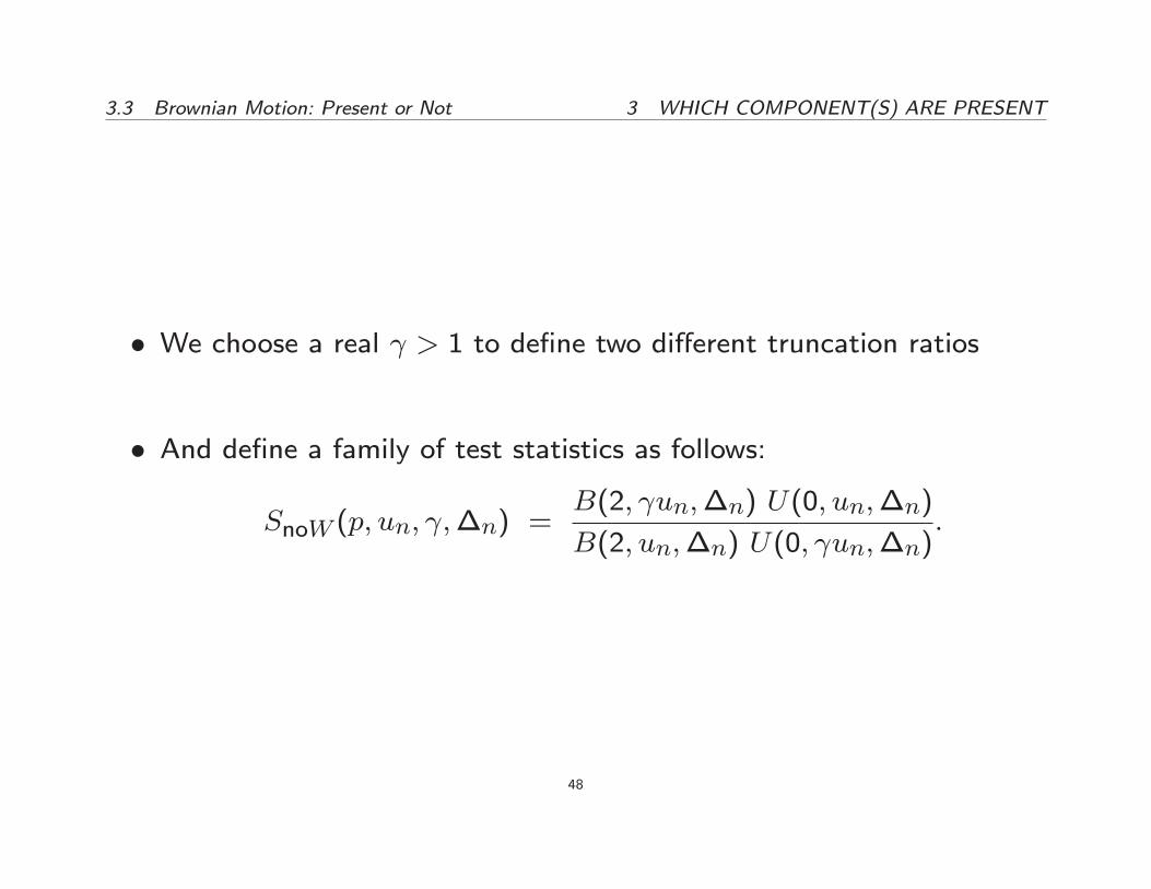
� We choose a real > 1 to de�ne two di�erent truncation ratios
� And de�ne a family of test statistics as follows:
SnoW (p; un; ;�n) =B(2; un;�n) U(0; un;�n)
B(2; un;�n) U(0; un;�n):
48

3.3 Brownian Motion: Present or Not 3 WHICH COMPONENT(S) ARE PRESENT
� To understand the construction of this test statistic, recall that in apower variation of order 2 the contributions from the Brownian and
jump components are of the same order.
� If the Brownian motion is present (H1 : WT )
{ Once that power variation is properly truncated, the Brownian mo-
tion will dominate it if it is present.
{ And the truncation can be chosen to be su�ciently loose that it
retains essentially all the increments of the Brownian motion at
cuto� level un and a fortiori un, thereby making the ratio of
the two truncated quadratic variations converge to 1 under the
alternative hypothesis.
49

3.3 Brownian Motion: Present or Not 3 WHICH COMPONENT(S) ARE PRESENT
� If the Brownian motion is not present (H0 : noWT )
{ Then the nature of the tail of jump distributions is such that the
di�erence in cuto� levels between un and un remains material no
matter how far we go in the tail
{ And the limit of the ratio B(2; un;�n)B(2;un;�n)
in SnoW will re ect it: it
will now be 2��.
{ Since absence of a Brownian motion is now the null hypothesis,
the issue for constructing a test is that this limit depends on the
unknown �:
50
3.3 Brownian Motion: Present or Not 3 WHICH COMPONENT(S) ARE PRESENT
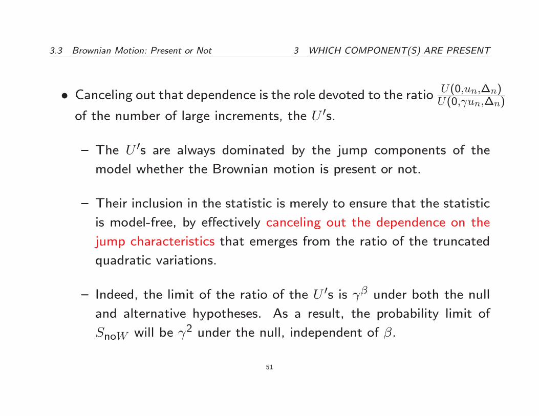
� Canceling out that dependence is the role devoted to the ratio U(0;un;�n)U(0; un;�n)
of the number of large increments, the U 0s.
{ The U 0s are always dominated by the jump components of themodel whether the Brownian motion is present or not.
{ Their inclusion in the statistic is merely to ensure that the statistic
is model-free, by e�ectively canceling out the dependence on the
jump characteristics that emerges from the ratio of the truncated
quadratic variations.
{ Indeed, the limit of the ratio of the U 0s is � under both the nulland alternative hypotheses. As a result, the probability limit of
SnoW will be 2 under the null, independent of �.
51
3.3 Brownian Motion: Present or Not 3 WHICH COMPONENT(S) ARE PRESENT
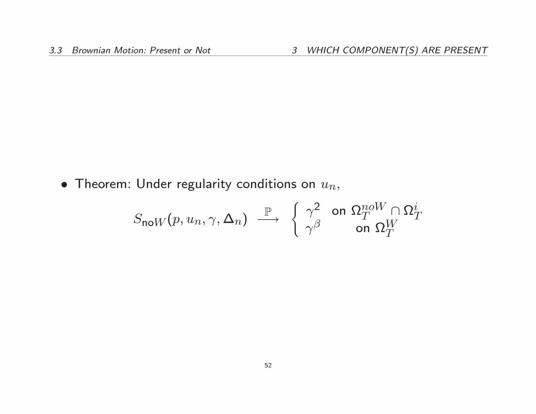
� Theorem: Under regularity conditions on un;
SnoW (p; un; ;�n)P�!
( 2 on noWT \ iT � on WT
52

4 THE RELATIVE MAGNITUDE OF THE COMPONENTS
4. The Relative Magnitude of the Components
� A typical \main sequence" star might be made of 90% hydrogen, 10%
helium and 0.1% everything else.
� Here, what is the relative magnitude of the two jump and the contin-uous components?
� We can answer this question using the same device.
� It makes sense to consider p = 2 since this is the power where all thecomponents are present together.
53
4 THE RELATIVE MAGNITUDE OF THE COMPONENTS
� We can then truncate to split the QV into its continuous and jump
components
� And not truncate to estimate the full QV:B(2;un;�n)B(2;1;�n) = % of QV due to the continuous component
1� B(2;un;�n)B(2;1;�n) = % of QV due to the jump component
� Alternative splitting of the QV based on bipower variation instead
of truncating: Barndor�-Nielsen and Shephard (2004), Huang and
Tauchen (2005), Andersen, Bollerslev and Diebold (2007).
54
4 THE RELATIVE MAGNITUDE OF THE COMPONENTS
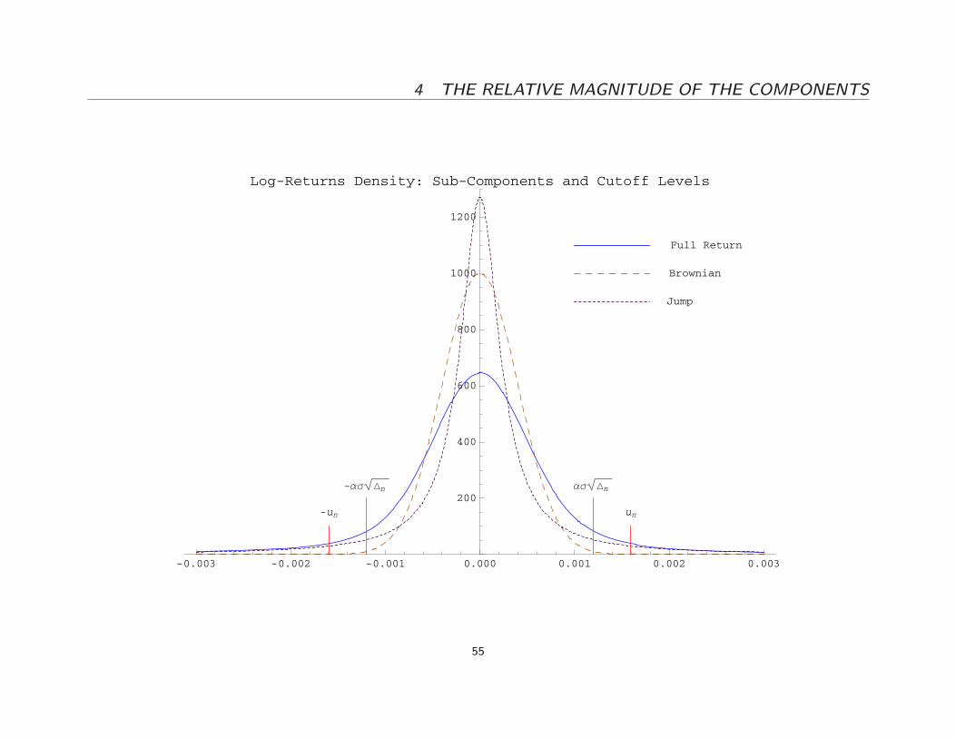
-0.003 -0.002 -0.001 0.000 0.001 0.002 0.003
200
400
600
800
1000
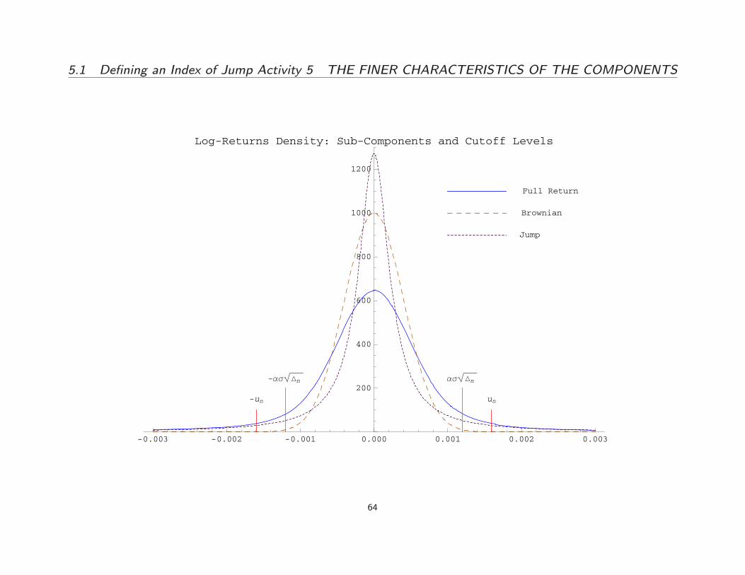
1200
Log-Returns Density: Sub-Components and Cutoff Levels
-un un
-ασ Δn ασ Δn
Full Return
Brownian
Jump
55
4 THE RELATIVE MAGNITUDE OF THE COMPONENTS
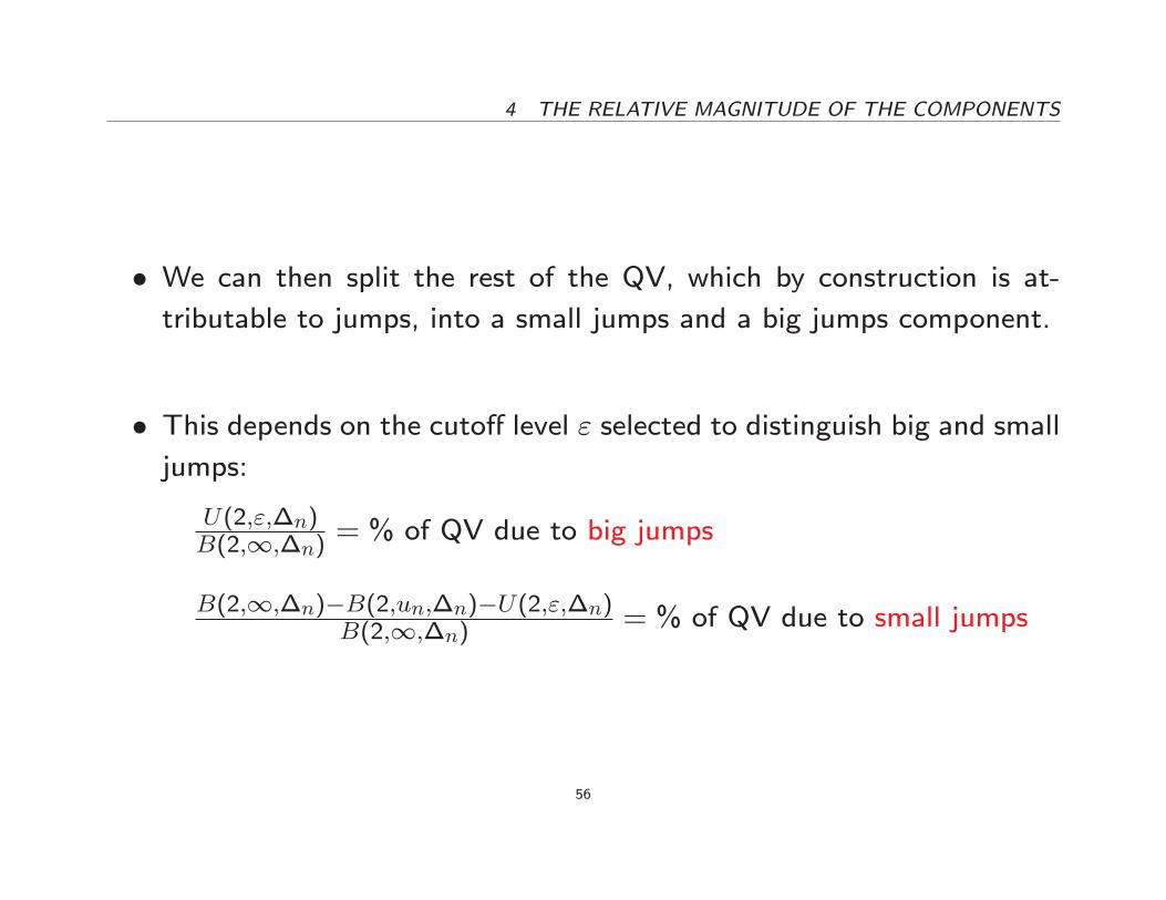
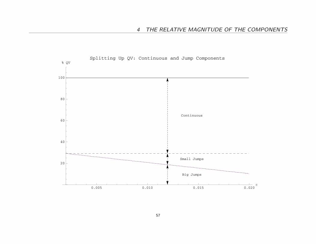
� We can then split the rest of the QV, which by construction is at-tributable to jumps, into a small jumps and a big jumps component.
� This depends on the cuto� level " selected to distinguish big and smalljumps:
U(2;";�n)B(2;1;�n) = % of QV due to big jumps
B(2;1;�n)�B(2;un;�n)�U(2;";�n)B(2;1;�n) = % of QV due to small jumps
56
4 THE RELATIVE MAGNITUDE OF THE COMPONENTS
0.005 0.010 0.015 0.020ε
20
40
60
80
100
% QVSplitting Up QV: Continuous and Jump Components
Continuous
Small Jumps
Big Jumps
57

5 THE FINER CHARACTERISTICS OF THE COMPONENTS
5. The Finer Characteristics of the Components
5.1. De�ning an Index of Jump Activity
� Recall B(p) = Ps�T j�Xsjp.
� De�ne IT = fp � 0 : B(p) <1g:
� Necessarily, the (random) set IT is of the form [�T ;1) or (�T ;1)for some �T (!) � 2, and 2 2 IT always.
58
5.1 De�ning an Index of Jump Activity 5 THE FINER CHARACTERISTICS OF THE COMPONENTS
� We call �T (!) the jump activity index for the path t 7! Xt(!) at time
T .
� We de�ne this index in analogy with the special case where X is a
L�evy process:
{ Then �T (!) = � does not depend on (!; T ), and it is also the
in�mum of all r � 0 such thatRfjxj�1g jxjr�(dx) <1, where � is
the L�evy measure
{ This property shows that, for a L�evy process, the jump activity
index coincides with the Blumenthal-Getoor index of the process.
{ In the further special case where X is a stable process, then � is
also the stable index of the process.
59

5.1 De�ning an Index of Jump Activity 5 THE FINER CHARACTERISTICS OF THE COMPONENTS
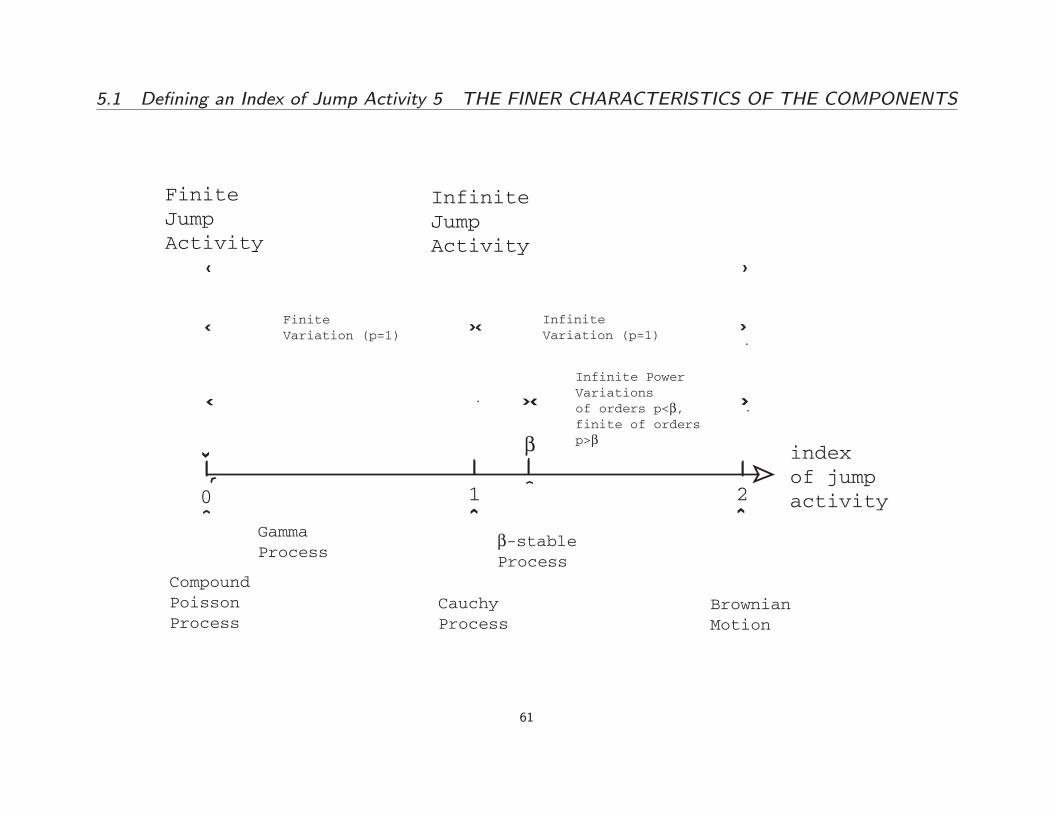
� � captures an essential qualitative feature of �, which is its level ofactivity: when � increases, the (small) jumps tend to become more
and more frequent.
{ Processes with �nite jump activity have � = 0:
{ Processes with in�nite jump activity may also have � = 0 if the
rate of divergence of the jump measure is sub-polynomial.
{ Processes with � 2 (0; 2) have in�nite jump activity
{ And the higher �; the more active the jumps.
� Brownian motion has � = 2 in the limit.
60
5.1 De�ning an Index of Jump Activity 5 THE FINER CHARACTERISTICS OF THE COMPONENTS
index of jumpactivity
β-stableProcess
β
0
FiniteJumpActivity
1 2
InfiniteJumpActivity
CompoundPoissonProcess
CauchyProcess
BrownianMotion
GammaProcess
FiniteVariation (p=1)
InfiniteVariation (p=1)
Infinite PowerVariationsof orders p<β, finite of ordersp>β
61

5.1 De�ning an Index of Jump Activity 5 THE FINER CHARACTERISTICS OF THE COMPONENTS
� The problem is made more challenging by the presence in X of a
continuous, or Brownian, martingale part:
{ � characterizes the behavior of � near 0:
{ Hence it is natural to expect that the small increments of the
process are going to be the ones that are most informative about
�:
{ But that is where the contribution from the continuous martingale
part of the process is inexorably mixed with the contribution from
the small jumps.
{ We need to see through the continuous part of the semimartingale
in order to say something about the number and concentration of
small jumps.
62

5.1 De�ning an Index of Jump Activity 5 THE FINER CHARACTERISTICS OF THE COMPONENTS
� So we are now looking in adi�erent range of the spectrum of returns
� Considering only returns that are larger than the cuto� un = ��$n forsome $ 2 (0; 1=2):
� This allows us to eliminate the increments due to the continuous com-ponent.
� We can then use all values of p; not just those p > 2:
63
5.1 De�ning an Index of Jump Activity 5 THE FINER CHARACTERISTICS OF THE COMPONENTS
-0.003 -0.002 -0.001 0.000 0.001 0.002 0.003
200
400
600
800
1000
1200
Log-Returns Density: Sub-Components and Cutoff Levels
-un un
-ασ Δn ασ Δn
Full Return
Brownian
Jump
64
5.2 Estimating Jump Activity 5 THE FINER CHARACTERISTICS OF THE COMPONENTS
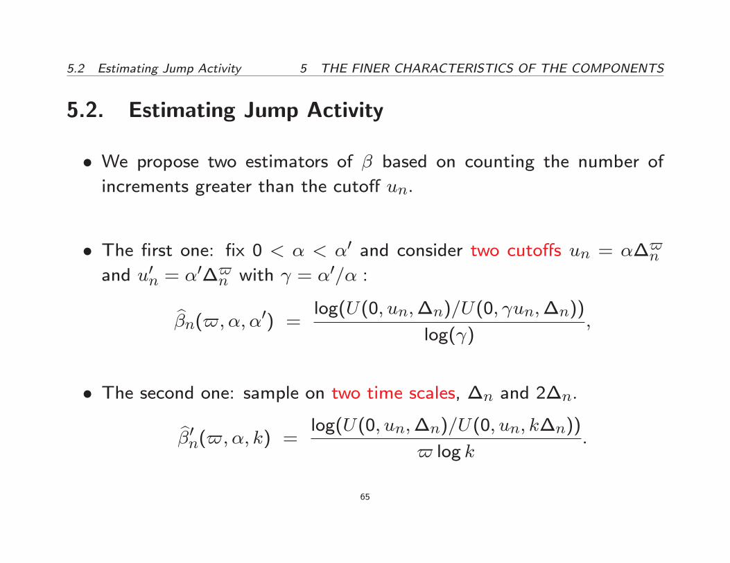
5.2. Estimating Jump Activity
� We propose two estimators of � based on counting the number of
increments greater than the cuto� un:
� The �rst one: �x 0 < � < �0 and consider two cuto�s un = ��$nand u0n = �
0�$n with = �0=� :
b�n($;�; �0) = log(U(0; un;�n)=U(0; un;�n))
log( );
� The second one: sample on two time scales, �n and 2�n.
b�0n($;�; k) = log(U(0; un;�n)=U(0; un; k�n))
$ log k:
65
5.2 Estimating Jump Activity 5 THE FINER CHARACTERISTICS OF THE COMPONENTS
� Given consistent estimators and with a CLT
� We could test various hypotheses, for instance whether � > 1 or � < 1which correspond to �nite or in�nite variation for X:
� Related methods: testing whether � = 1 (Cont and Mancini (2009)),
testing whether � = 2 or � < 2 (Tauchen and Todorov (2009)).
66
6 SUMMARY: (P;U;�)
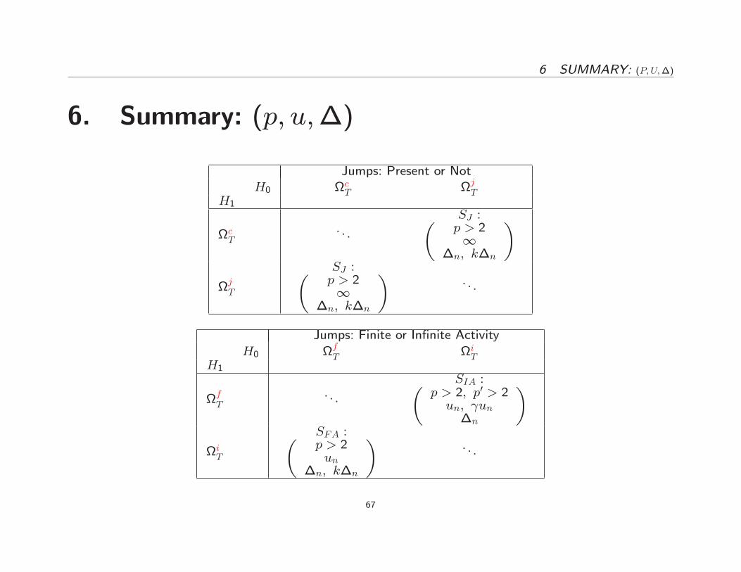
6. Summary: (p; u;�)
Jumps: Present or NotH0 cT jT
H1
cT. . .
SJ :�p > 21
�n; k�n
�jT
SJ :�p > 21
�n; k�n
�. . .
Jumps: Finite or In�nite Activity
H0 fT iTH1
fT. . .
SIA :�p > 2; p0 > 2un; un�n
�iT
SFA :�p > 2un
�n; k�n
�. . .
67
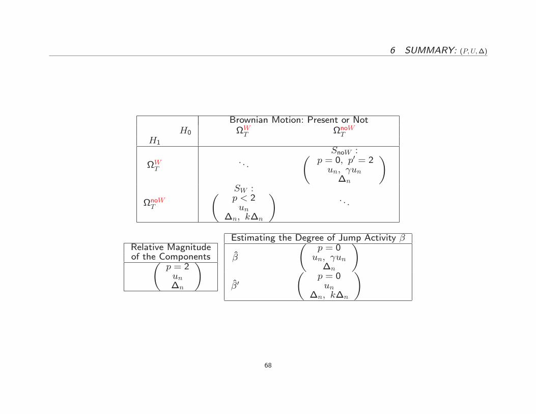
6 SUMMARY: (P;U;�)
Brownian Motion: Present or NotH0 WT noWT
H1
WT. . .
SnoW :�p = 0; p0 = 2un; un�n
�noWT
SW :�p < 2un
�n; k�n
�. . .
Relative Magnitudeof the Components�
p = 2un�n
�Estimating the Degree of Jump Activity �
�
�p = 0un; un�n
��0
�p = 0un
�n; k�n
�
68
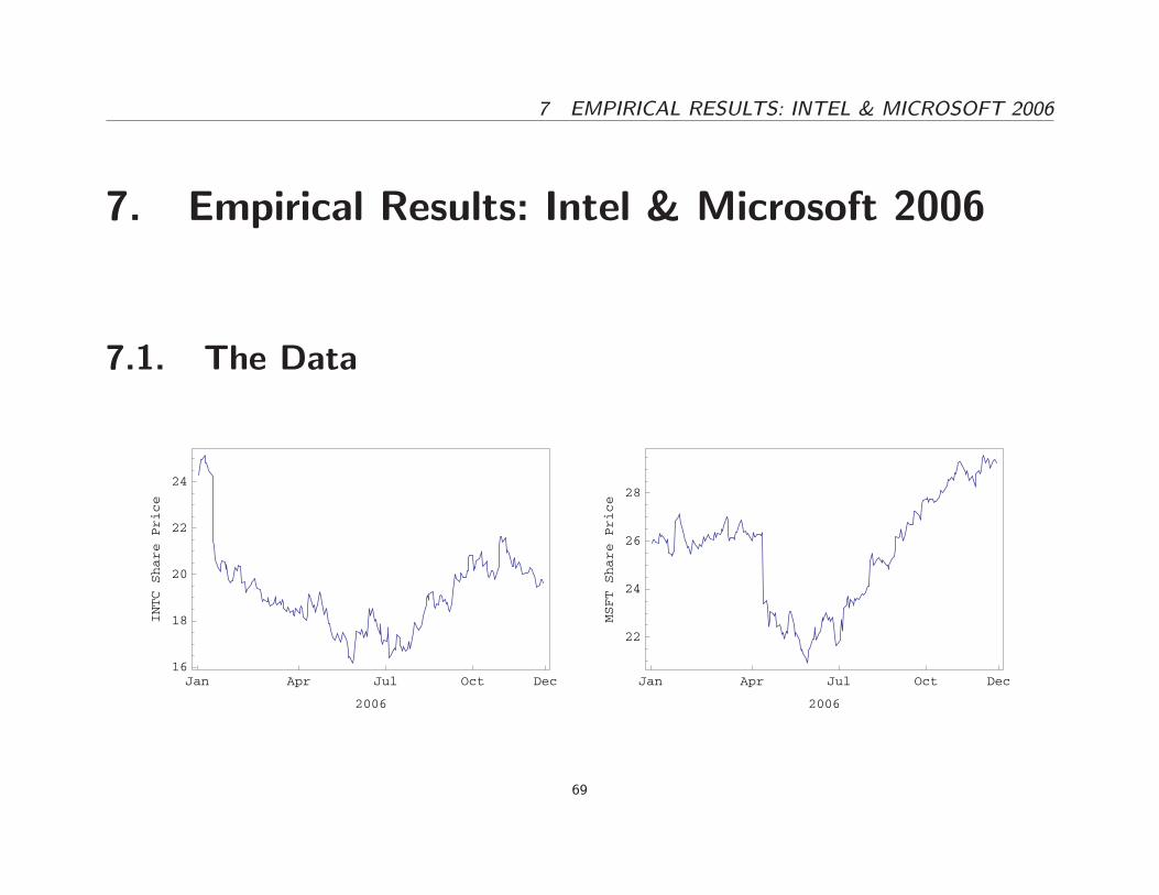
7 EMPIRICAL RESULTS: INTEL & MICROSOFT 2006
7. Empirical Results: Intel & Microsoft 2006
7.1. The Data
Jan Apr Jul Oct Dec16
18
20
22
24
2006
INTCSharePrice
Jan Apr Jul Oct Dec
22
24
26
28
2006
MSFTSharePrice
69
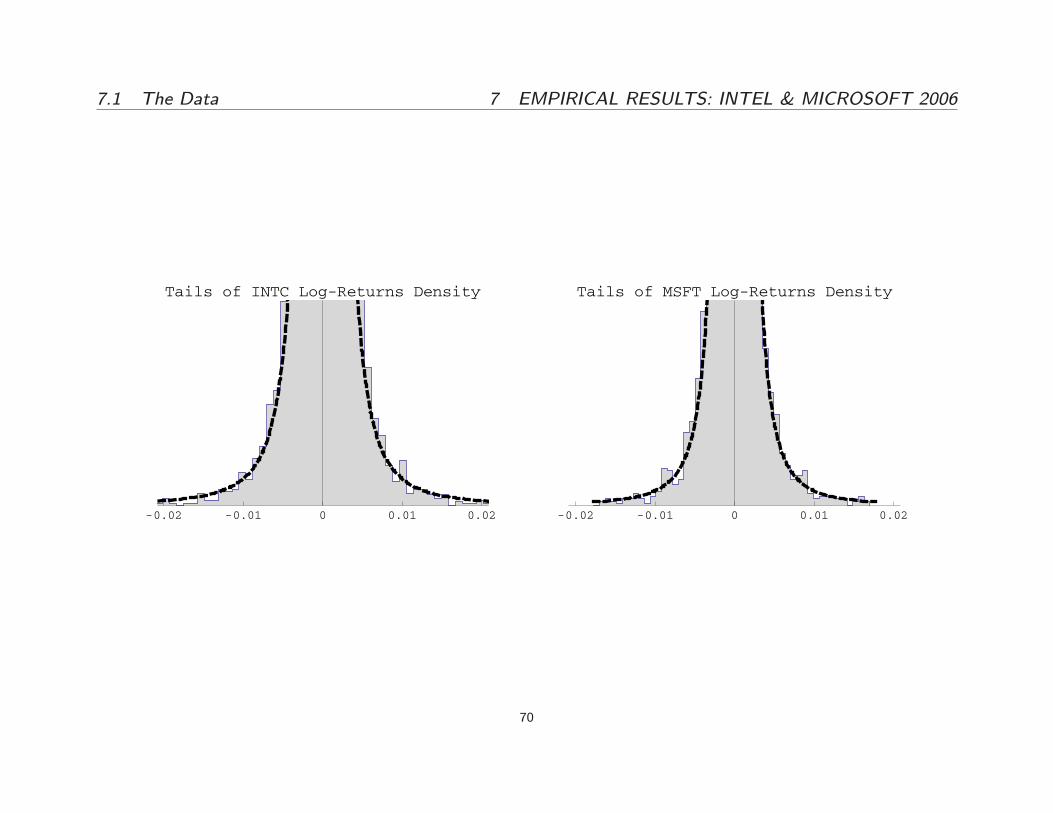
7.1 The Data 7 EMPIRICAL RESULTS: INTEL & MICROSOFT 2006
-0.02 -0.01 0 0.01 0.02
Tails of INTC Log-Returns Density
-0.02 -0.01 0 0.01 0.02
Tails of MSFT Log-Returns Density
70
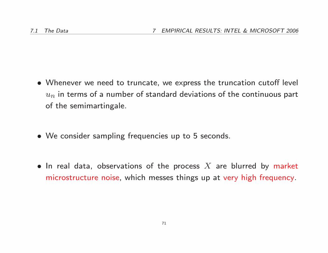
7.1 The Data 7 EMPIRICAL RESULTS: INTEL & MICROSOFT 2006
� Whenever we need to truncate, we express the truncation cuto� levelun in terms of a number of standard deviations of the continuous part
of the semimartingale.
� We consider sampling frequencies up to 5 seconds.
� In real data, observations of the process X are blurred by market
microstructure noise, which messes things up at very high frequency.
71
7.2 Jumps: Present or Not 7 EMPIRICAL RESULTS: INTEL & MICROSOFT 2006
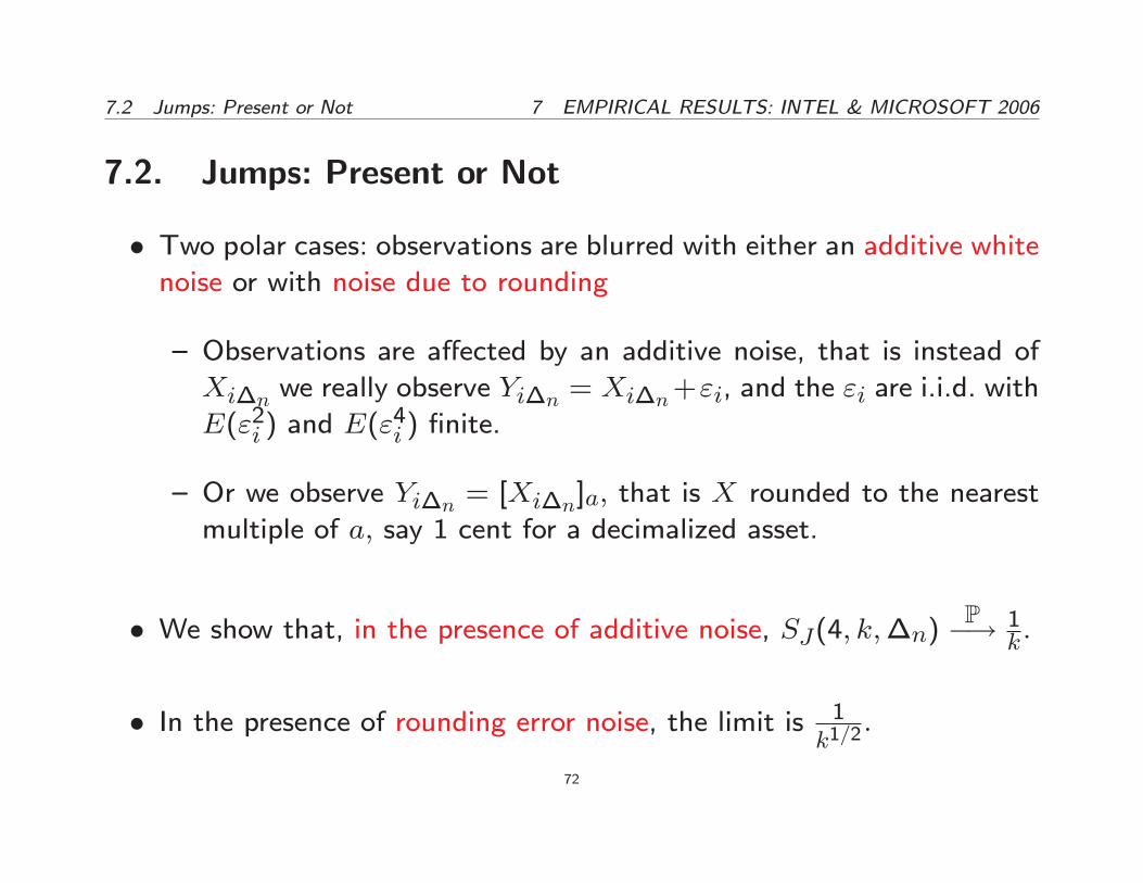
7.2. Jumps: Present or Not
� Two polar cases: observations are blurred with either an additive whitenoise or with noise due to rounding
{ Observations are a�ected by an additive noise, that is instead ofXi�n we really observe Yi�n = Xi�n+"i, and the "i are i.i.d. with
E("2i ) and E("4i ) �nite.
{ Or we observe Yi�n = [Xi�n]a; that is X rounded to the nearest
multiple of a; say 1 cent for a decimalized asset.
� We show that, in the presence of additive noise, SJ(4; k;�n)P�! 1
k:
� In the presence of rounding error noise, the limit is 1k1=2
:
72
7.2 Jumps: Present or Not 7 EMPIRICAL RESULTS: INTEL & MICROSOFT 2006
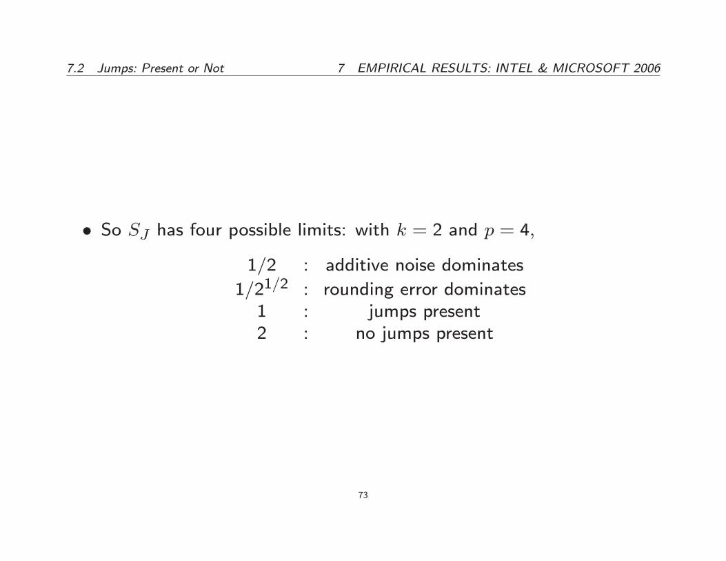
� So SJ has four possible limits: with k = 2 and p = 4;
1=2 : additive noise dominates
1=21=2 : rounding error dominates1 : jumps present2 : no jumps present
73
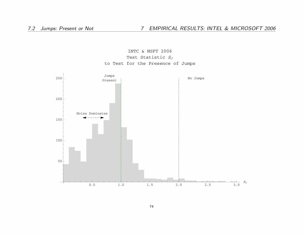
7.2 Jumps: Present or Not 7 EMPIRICAL RESULTS: INTEL & MICROSOFT 2006
0.5 1.0 1.5 2.0 2.5 3.0SJ
50
100
150
200
250
INTC & MSFT 2006
Test Statistic SJto Test for the Presence of Jumps
Noise Dominates
Jumps
PresentNo Jumps
74
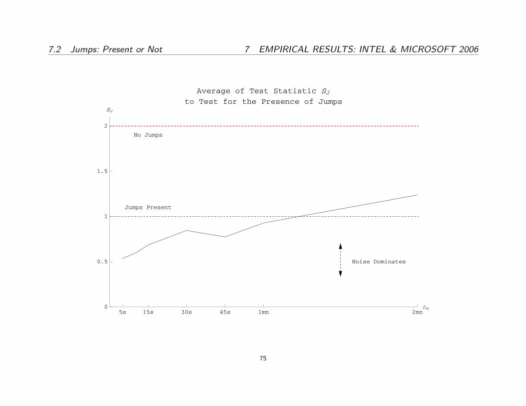
7.2 Jumps: Present or Not 7 EMPIRICAL RESULTS: INTEL & MICROSOFT 2006
5s 15s 30s 45s 1mn 2mnΔn0
0.5
1
1.5
2
SJ
Average of Test Statistic SJto Test for the Presence of Jumps
Noise Dominates
Jumps Present
No Jumps
75
7.3 Jumps: Finite or In�nite Activity 7 EMPIRICAL RESULTS: INTEL & MICROSOFT 2006
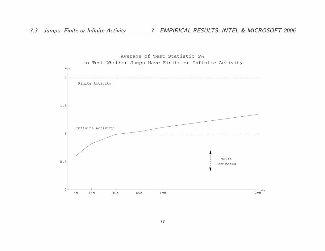
7.3. Jumps: Finite or In�nite Activity
0.5 1.0 1.5 2.0 2.5 3.0SFA
100
200
300
400
INTC & MSFT 2006
Test Statistic SFAto Test Whether Jumps Have Finite or Infinite Activity
Noise
Dominates
Infinite
Activity
Jumps
Finite
Activity
Jumps
76
7.3 Jumps: Finite or In�nite Activity 7 EMPIRICAL RESULTS: INTEL & MICROSOFT 2006
5s 15s 30s 45s 1mn 2mnΔn0
0.5
1
1.5
2
SFA
Average of Test Statistic SFAto Test Whether Jumps Have Finite or Infinite Activity
Noise
Dominates
Infinite Activity
Finite Activity
77

7.4 Brownian Motion: Present or Not 7 EMPIRICAL RESULTS: INTEL & MICROSOFT 2006
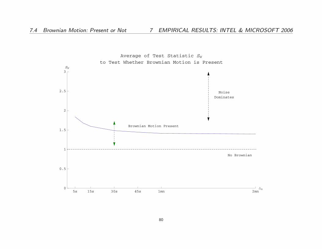
7.4. Brownian Motion: Present or Not
� Market microstructure noise with either an additive white noise or withnoise due to rounding, the respective limits of SW become 2 and 21=2
with k = 2:
� SW has four possible limits:
1 : No Brownian motion
k1�p=2 : Brownian motion present
k1=2 : rounding error dominatesk : additive noise dominates
78
7.4 Brownian Motion: Present or Not 7 EMPIRICAL RESULTS: INTEL & MICROSOFT 2006
0.5 1.0 1.5 2.0 2.5 3.0SW
50
100
150
200
INTC & MSFT 2006
Test Statistic SWto Test Whether Brownian Motion is Present
Noise Dominates
Brownian Motion
Present
No
Brownian
79
7.4 Brownian Motion: Present or Not 7 EMPIRICAL RESULTS: INTEL & MICROSOFT 2006
5s 15s 30s 45s 1mn 2mnΔn0
0.5
1
1.5
2
2.5
3SW
Average of Test Statistic SWto Test Whether Brownian Motion is Present
Noise
Dominates
Brownian Motion Present
No Brownian
80
7.5 QV Relative Magnitude 7 EMPIRICAL RESULTS: INTEL & MICROSOFT 2006
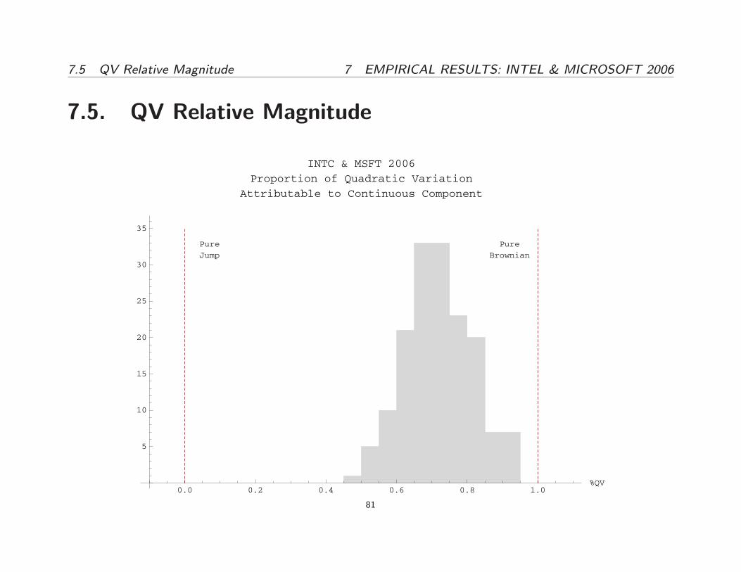
7.5. QV Relative Magnitude
0.0 0.2 0.4 0.6 0.8 1.0%QV
5
10
15
20
25
30
35
INTC & MSFT 2006
Proportion of Quadratic Variation
Attributable to Continuous Component
Pure
Jump
Pure
Brownian
81
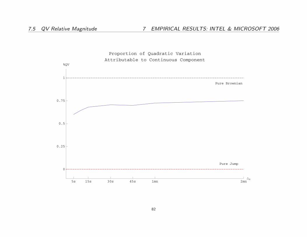
7.5 QV Relative Magnitude 7 EMPIRICAL RESULTS: INTEL & MICROSOFT 2006
5s 15s 30s 45s 1mn 2mnΔn
0
0.25
0.5
0.75
1
%QV
Proportion of Quadratic Variation
Attributable to Continuous Component
Pure Brownian
Pure Jump
82
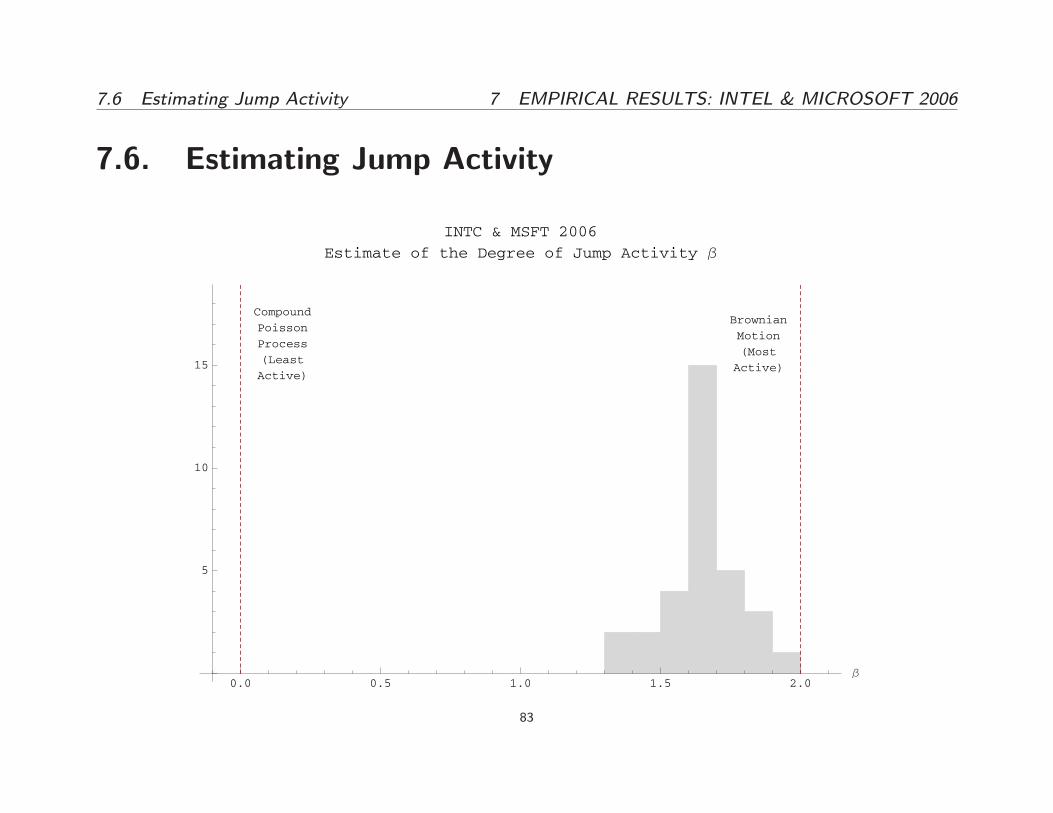
7.6 Estimating Jump Activity 7 EMPIRICAL RESULTS: INTEL & MICROSOFT 2006
7.6. Estimating Jump Activity
0.0 0.5 1.0 1.5 2.0β
5
10
15
INTC & MSFT 2006
Estimate of the Degree of Jump Activity β
Compound
Poisson
Process
(Least
Active)
Brownian
Motion
(Most
Active)
83
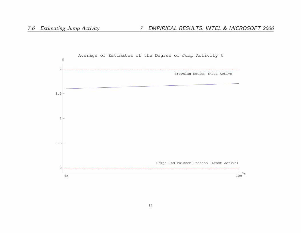
7.6 Estimating Jump Activity 7 EMPIRICAL RESULTS: INTEL & MICROSOFT 2006
5s 10sΔn
0
0.5
1
1.5
2
βAverage of Estimates of the Degree of Jump Activity β
Compouund Poisson Process (Least Active)
Brownian Motion (Most Active)
84
8 CONCLUSIONS
8. Conclusions
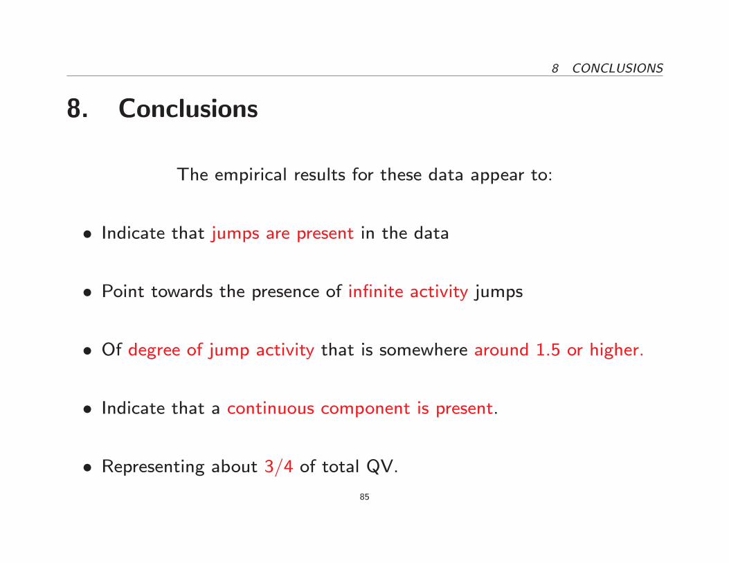
The empirical results for these data appear to:
� Indicate that jumps are present in the data
� Point towards the presence of in�nite activity jumps
� Of degree of jump activity that is somewhere around 1.5 or higher.
� Indicate that a continuous component is present.
� Representing about 3/4 of total QV.85
8 CONCLUSIONS
� Pros
{ Uni�ed methodology to address all these speci�cation questions in
a common framework
{ Symmetric treatment of null and alternative in each case, including
distribution theory
{ Model-free
{ Extremely simple to implement
{ Impact of the noise on the statistics is characterized
86
8 CONCLUSIONS
� Cons
{ Not necessarily the optimal approach for each one of these ques-
tions taken individually.
{ Requires high frequency data (particularly the estimation of �)
{ Still to do: a full development of noise-robust statistics.
87


![p4 20 Yacine Zellouf 1[1]](https://img.pdfslide.net/doc/110x75/577cd75d1a28ab9e789eca1d/p4-20-yacine-zellouf-11.jpg)