Research ArticleAnatomical Modeling of Brain Vasculature in Two-PhotonMicroscopy by Generalizable Deep Learning

Waleed Tahir ,1 Sreekanth Kura ,2 Jiabei Zhu,1 Xiaojun Cheng,2 Rafat Damseh ,3

Fetsum Tadesse ,2 Alex Seibel ,2 Blaire S. Lee,2,4 Frédéric Lesage ,3 Sava Sakadžic,5

David A. Boas ,1,2,6 and Lei Tian 1,6

1Department of Electrical and Computer Engineering, Boston University, Boston, MA, USA2Department of Biomedical Engineering, Boston University, Boston, MA, USA3Biomedical Engineering Institute, École Polytechnique de Montréal, Montréal, QC, Canada4Institute of Neurological Sciences and Psychiatry, Hacettepe University, Ankara, Turkey5Department of Radiology, Massachusetts General Hospital, Harvard Medical School, Charlestown, USA6Neurophotonics Center, Boston University, Boston, MA, USA

Correspondence should be addressed to Lei Tian; leitian@bu.edu

Received 14 June 2020; Accepted 12 November 2020; Published 18 January 2021

Copyright © 2020 Waleed Tahir et al. Exclusive Licensee Science and Technology Review Publishing House. Distributed under aCreative Commons Attribution License (CC BY 4.0).

Objective and Impact Statement. Segmentation of blood vessels from two-photon microscopy (2PM) angiograms of brains hasimportant applications in hemodynamic analysis and disease diagnosis. Here, we develop a generalizable deep learningtechnique for accurate 2PM vascular segmentation of sizable regions in mouse brains acquired from multiple 2PM setups. Thetechnique is computationally efficient, thus ideal for large-scale neurovascular analysis. Introduction. Vascular segmentationfrom 2PM angiograms is an important first step in hemodynamic modeling of brain vasculature. Existing segmentation methodsbased on deep learning either lack the ability to generalize to data from different imaging systems or are computationallyinfeasible for large-scale angiograms. In this work, we overcome both these limitations by a method that is generalizable tovarious imaging systems and is able to segment large-scale angiograms. Methods. We employ a computationally efficient deeplearning framework with a loss function that incorporates a balanced binary-cross-entropy loss and total variation regularizationon the network’s output. Its effectiveness is demonstrated on experimentally acquired in vivo angiograms from mouse brains ofdimensions up to 808 × 808 × 702 μm. Results. To demonstrate the superior generalizability of our framework, we train on datafrom only one 2PM microscope and demonstrate high-quality segmentation on data from a different microscope without anynetwork tuning. Overall, our method demonstrates 10× faster computation in terms of voxels-segmented-per-second and 3×larger depth compared to the state-of-the-art. Conclusion. Our work provides a generalizable and computationally efficientanatomical modeling framework for brain vasculature, which consists of deep learning-based vascular segmentation followed bygraphing. It paves the way for future modeling and analysis of hemodynamic response at much greater scales that wereinaccessible before.

1. Introduction

The hemodynamic response to neural activation has becomea vital tool in understanding brain function and pathologies[1]. In particular, measuring vascular dynamics has provedto be important for the early diagnosis of critical cerebrovas-cular and neurological disorders, such as stroke and Alzhei-mer’s disease [2]. Existing tools for the measurement ofcerebral vascular dynamics rely on functional imaging tech-

niques, for example, functional magnetic resonance imaging(fMRI), positive emission tomography (PET), and opticalimaging [1, 3]. Importantly, mathematical models have beenproposed for these neuroimaging methods, which providevaluable insight into the relation between the measured sig-nals, and the underlying physiological parameters, such ascerebral blood flow, oxygen consumption, and rate of metab-olism [4–7]. These mathematical models often require atopological representation of the blood vessels as a graph of

AAASBME FrontiersVolume 2021, Article ID 8620932, 12 pageshttps://doi.org/10.34133/2021/8620932

spatially distributed nodes, connected via edges [5, 7]. Thesevascular graphs are usually estimated from two-photonmicroscopy (2PM) angiograms of the mouse brain [5], andsegmentation of blood vessels is generally the first step in thisprocess [8]. Vascular segmentation from cerebral 2PM angio-grams, however, is a challenging task, especially for in vivoimaging. Current state-of-the-art methods for this task [9,10] suffer from limited computational speed, restricting theirusefulness to only small-scale volumetric regions of the brain.Furthermore, due to rapid deterioration of measurement con-trast with imaging depth in 2PM, these methods have beenunable to demonstrate effective segmentation for vasculaturedeep beneath the brain surface. In this work, we address theselimitations and present a computationally efficient frameworkfor 2PM vascular segmentation that allows us to effectivelyprocess much larger regions of the mouse brain compared toexisting methods at significantly faster computation speed interms of voxels segmented per second. Our method also dem-onstrates accurate segmentation for significantly deeper vas-culature compared to the state-of-the-art.

Vascular segmentation involves assigning a binary labelto each voxel of the input angiogram to indicate whether ornot it is part of a blood vessel. This task is challenging, espe-cially when dealing with 2PM angiograms, as the measure-ment contrast decreases sharply with imaging depth due tomultiple scattering and background fluorescence [11]. Addi-tional sources of measurement noise include motion artifactcorruption during in vivo imaging, large pial vessels on thecortical surface, and densely packed vasculature, makingthe segmentation task nontrivial. In the presence of thesechallenges, a number of techniques have been employed forvascular segmentation, including methods based on the Hes-sian matrix [12, 13], tracing [14], optimally oriented flux[15], and geometric flow [16]. However, in practice, thesemethods demonstrate limited segmentation quality [8].

In recent years, techniques based on deep learning haveshown significant improvement over traditional methodsfor 2PM vascular segmentation [8–10, 17]. One of the firstworks in this line was presented by Teikari et al. in their pre-print study [17], who proposed a hybrid 2D/3D deep neuralnetwork (DNN) for the segmentation task. Their method uti-lized angiograms with shallow imaging depths (less than100μm) and was limited by computation speed. The segmen-tation quality was improved upon by Haft et al. [10] by usingan end-to-end 3D segmentation DNN. This model, however,similar to Teikari et al., was also limited by slow computationand required about one month to train on a dataset consist-ing of one annotated angiogram of dimensions 292 × 292 ×200 μm. Damseh et al. [8] improved upon this limitationand were able to process much larger datasets with fastercomputation speed in terms of voxels segmented per second.Their framework used a DNN based on the DenseNet archi-tecture [18], which processed the 3D angiograms by seg-menting 2D slices one-by-one, and demonstrated bettersegmentation quality compared to previous methods. How-ever, this DNN did not generalize with respect to variousimaging setups, i.e., it performed good segmentation onlyfor 2PM angiograms acquired on the same setup as thetraining data. Ideally, one would like to be able to segment

angiograms from any 2PM microscope once the network hasbeen trained. In order to overcome this limitation, Gur et al.[9] recently proposed an unsupervisedDNNbased on the activecontours method and demonstrated improved generalizationcapability compared to supervisedmodels [8, 10, 17], with fastersegmentation speed. However, this method still suffers fromexcessive training and inference times and high computationalcost. Furthermore, the lack of “supervised” information makesit difficult to segment deep vasculature, as severe noise corrup-tion makes the task very challenging, even when using activecontours [19]. These challenges limited its effectiveness tosmall-scale angiograms, with up to 200μm imaging depth.Therefore, there is a need for a vascular segmentation methodthat is not only able to generalize to different 2PM imagingsetups but is also fast and computationally efficient, to cope withthe processing needs of large-scale angiograms.

In this work, we propose a novel deep learning methodfor vascular segmentation of cerebral 2PM angiograms,which overcomes the aforementioned limitations of the exist-ing techniques and demonstrates state-of-the-art segmenta-tion performance. Our contribution here is three-fold. First,we present a novel application of a total variation (TV) regu-larized loss function for 2PM vascular segmentation. Theproposed loss function combines the “supervised” informa-tion from training data acquired on a single imaging setup,with an “unsupervised” regularization term that penalizesthe total variation of the DNN output. This regularizationencourages piece-wise continuity in the final segmentationand improves the generalization ability of the trained DNNto different imaging setups, without the need of excessivetraining data, transfer learning [20], or domain transfer[21]. The TV-regularized loss also makes the DNN signifi-cantly more robust to mislabeled ground-truth annotations.This is particularly useful for large-scale 2PM vascular angio-grams where significant noise in deep vasculature makes pre-cise ground-truth annotation very challenging, even forhuman annotators, making the ground-truth data prone tomislabeling. The TV penalty also imparts inherent denoisingcapability to the trained network, eliminating the need forany postprocessing. Our second contribution is a novel pre-processing method, which aids in the generalization by mak-ing the histogram of an arbitrary test angiogram similar tothat of training data, in addition to reducing its noise. Wedemonstrate the effectiveness of this preprocessing methodto improve segmentation quality, not only with our proposedmethod but also with some existing 2PM vascular segmenta-tion techniques. Our third contribution is the novel applica-tion of an extremely lightweight, end-to-end 3D, DNN for2PM vascular segmentation, which is able to demonstratean order of magnitude faster segmentation, compared tothe current state-of-the-art [9], in terms of voxels segmentedper second. This enables us to perform segmentation on sig-nificantly larger regions in several mouse brains, thusenabling large-scale in vivo neurovascular analysis. To illus-trate this unique capability, we demonstrate segmentationon an 808 × 808 × 702 μm volume in less than 2.5 seconds.

Following vascular segmentation from our DNN model,we perform graph extraction on the binary segmentationmap using a recently developed method based on the

2 BME Frontiers

Laplacian flow dynamics [22]. Importantly, we show that oursegmentation results in better graph modeling of the vascula-ture across large volumes compared to other segmentationtechniques.

Overall, we present a new high-speed and computation-ally efficient anatomical modeling framework for the brainvasculature, which consists of deep learning-based vascularsegmentation followed by graphing. Our work paves theway for future modeling and analysis of hemodynamicresponse at much greater scales that were inaccessible before.To facilitate further advancements in this field of research, wehave made our DNN architecture, dataset, and trainedmodels publicly available at https://github.com/bu-cisl/2PM_Vascular_Segmentation_DNN.

2. Results

2.1. System Framework. The deep learning-based vasculatureanatomical modeling pipeline is shown in Figure 1(a). Thismodular framework takes 2PM angiograms of live mousebrain as the input, performs segmentation of blood vesselsusing a novel 3D DNN, and finally extracts a vascular graphfrom the network’s prediction. The DNN (Figure 1(b), S7),detailed in Section 4.3, is of critical importance in this pipe-line and is our primary contribution, along with the novelapplication of a TV-regularized loss function for 2PM vascu-lar segmentation, detailed in Section 4.4. This network is firsttrained to minimize the discrepancy between manuallyannotated ground-truth segmentation and its own prediction(Figure 1(b)). During this training process, the network isexposed to challenging regions in 2PM angiograms in orderto improve its vessel recovery from poor quality images.Some examples of such regions include deep 2PM measure-

ments with low signal contrast (Figure 2(a)) and pial vesselocclusions (Figure 2(a), red circle). In addition, we use largeinput angiogram patches of size 128 × 128 × 128 voxels, inconjunction with a network optimized for computationspeed, allowing us faster segmentation on significantly largerangiograms compared to state-of-the-art methods [9, 10].Once trained, this network provides segmentation of 2PMangiograms in a feed-forward manner (Figure 1(c)) that out-performs the state-of-the-art methods as detailed below.

2.2. Segmentation Performance Analysis. To evaluate our seg-mentation approach, we first visually compare the predictedvessel segmentation from our DNN with the ground truth,a traditional Hessian matrix approach [3], and a recentlydeveloped DNN model [8] in Figure 3. Our method outper-forms both these techniques in terms of segmentation qual-ity, especially for vessels deep beneath the cortical surface.The Hessian matrix approach identifies tubular structuresby an enhancement function based on Hessian eigenvalues.While it recovers most of the vessels closer to the surface, itperforms poorly in this regard for deeper vessels, due to sig-nificantly higher measurement noise in the angiogram,which makes it difficult to distinguish between the vesselsand the surrounding noisy background. Damseh et al. [8]use a DenseNet architecture [18] to perform vascular seg-mentation in a 2D slice-wise manner. Although their net-work performs better than the Hessian approach, it alsosuffers from bad segmentation for deeper vessels and ignores3D context due to the slice-wise processing. A significantadvantage that the proposed method possesses, comparedto these techniques, is the TV-regularized loss function,which penalizes the variation of the DNN output, thusimparting inherent denoising capability to the network and

Measured angiogram 3D segmentation 3D graph

Weightoptimization

Trainingangiograms

Ground truthsegmentations

Test angiogram

Predictedsegmentation

DNNDNN

Training stage Segmentation stage

(trained)

Segmentationnetwork

2PMacquisition

Graphextraction

(a)

(b) (c)

Figure 1: Framework for vascular modeling. (a) Two-photon microscopy (2PM) is used to acquire cerebral angiographic data on a livespecimen via in vivo imaging. This is followed by binary vascular segmentation of the 2PM angiogram. Finally, the 3D graph of thevasculature is computed from the segmentation map. In this paper, we present the segmentation method in detail, which is able to processlarge-scale 2PM angiograms. (b) A deep neural network (DNN) is used for segmentation which is first trained using annotatedangiograms. During this process, the network weights are iteratively adjusted for accurate vessel segmentation. (c) After the training iscomplete, the optimized network can be used in a feed-forward manner for segmentation on unseen angiograms.

3BME Frontiers

improving its segmentation for deep vessels. In addition, theproposed DNN also performs end-to-end 3D processing ofdata, which takes into account the 3D context of the vascula-ture. Thus, the segmentation from our method maintains a

greater overlap of the prediction and ground truth comparedto other methods, out to 606μm (Figures 3(b)–3(d)). Theseresults indicate a 3× depth improvement using our approachover the current state-of-the-art methods. Since these largeimaging depths also exhibit poor signal-to-background ratios(SBR) (Figure 2), our DNN model also provides visuallysuperior performance under low signal contrast imagingconditions. As discussed below, we quantify these improve-ments using a comprehensive set of metrics to holisticallyevaluate the vascular segmentation performance.

Overlap-based metrics are the most widely used metricsto evaluate vessel segmentation algorithms, which are com-puted based on analyzing the voxel overlap between theground truth and the prediction. For example, sensitivityand specificity represent the respective percentage of theforeground and background voxels that are correctly recov-ered in the prediction. The Jaccard index computes the inter-section over the union of the prediction and the groundtruth, representing similarity based on percentage overlap.The Dice index is very similar to the Jaccard index, and thetwo are strongly positively correlated. Generally, such met-rics only compare the physical overlap between the groundtruth and the predicted segmentation without consideringthe underlying morphological shapes of the object [23]. Thisfactor makes overlap-based metrics ill-suited for delimitingcomplex boundaries like blood vessels, since they will prefer-entially correct larger vessels occupying more of the volumewhile ignoring the smaller, yet important capillaries in thevasculature. In addition, these metrics suffer from inherentbiases towards one segmentation class or the other. Forexample, the Jaccard index, the Dice coefficient, and sensitiv-ity are insensitive to true negative predictions, making themprimarily indicative of positive class performance. On theother hand, specificity is insensitive to true positive predic-tions, thus primarily indicative of negative class performance.Accuracy is subject to class imbalance, i.e., when one type ofclass labels are significantly more abundant than the rest,accuracy becomes more indicative of the abundant class. Thisproblem is particularly prevalent in vascular segmentation[24]. As an example, our manually segmented 2PM angio-grams contain more than 96% background tissue voxels

566-606 𝜇m286-326 𝜇m6-46 𝜇m

160 𝜇m

Gro

und

trut

hO

urs

Dam

seh

et. a

l. [8

]Je

rman

et. a

l. [1

3]

2PM measurement

(a) (b) (c) (d)

SegmentationOverlap

x xz

y

y

Figure 3: Large-scale 2PM vascular segmentation. (a) 3Drenderings of segmentation on the test angiogram. (b)-(d)Maximum intensity projections (MIPs) of binary segmentationoverlaid on 2PM measurement. Each MIP represents 40μmphysical depth and 20 discrete slices along the z-axis. MIPs forthree different depth ranges are presented to show the effect ofaxial depth on segmentation performance. We demonstrate goodsegmentation for vasculature up to 606μm, despite a significantincrease in background noise associated with 2PM.

Increasing depth

700 𝜇m400 𝜇m30 𝜇m

0Sign

al to

bac

kgro

und

ratio

(dB)

200–40

–20

20

40

60

0

400 600 800Imaging depth in 𝜇m

(a) (b)

Figure 2: Deterioration of two-photon microscopy signal with imaging depth. (a) Visual contrast decreases for deeper vasculature due to lossof illumination focus with increased imaging depth, and higher background fluorescence due to increased laser power. Large pial vessels onthe surface cast shadows underneath, as shown by the encircled region, making vessel detection challenging. (b) The signal to backgroundratio (SBR) of the angiogram decreases rapidly going deeper into the brain tissue.

4 BME Frontiers

and less than 4% foreground vessel voxels, indicating animbalance ratio of more than 24.

To overcome these shortcomings, we further quantifyour DNN performance using the correlation-based Mat-thew’s correlation coefficient (MCC) metric; two morpholog-ical similarity-based metrics, namely, Hausdorff distance(HD) and Modified Hausdorff distance (MHD); and agraph-based metric length correlation (LC). MCC is particu-larly suited for highly imbalanced data [25] since it is unbi-ased towards any class and gives the same value between -1and 1, even when negative and positive classes are swapped.A score of 1 means perfect correlation, 0 means uncorrelatedand the classifier is akin to random guessing, and -1 meansperfect negative correlation. HD measures the extent of mor-phological similarity between the prediction and groundtruth, i.e., how visually similar their shapes are. This metricis suitable for data involving complex contours, e.g., bloodvessels [23]. MHD is a variant of HD and is more robust tothe outliers and noise. LC is a graph-based metric, whichwe derive from the length metric in [26], and is specificallysuitable for vascular segmentation. It measures the degreeof coincidence between the predicted and the ground truthsegmentations in terms of the total length. Since accurategraph extraction is the eventual goal for our segmentationpipeline, LC is a particularly well-suited metric forcomparison.

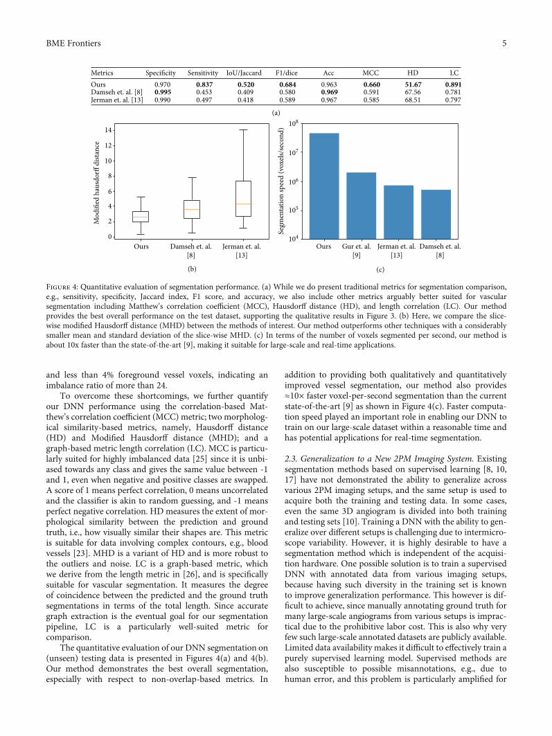
The quantitative evaluation of our DNN segmentation on(unseen) testing data is presented in Figures 4(a) and 4(b).Our method demonstrates the best overall segmentation,especially with respect to non-overlap-based metrics. In

addition to providing both qualitatively and quantitativelyimproved vessel segmentation, our method also provides≈10× faster voxel-per-second segmentation than the currentstate-of-the-art [9] as shown in Figure 4(c). Faster computa-tion speed played an important role in enabling our DNN totrain on our large-scale dataset within a reasonable time andhas potential applications for real-time segmentation.

2.3. Generalization to a New 2PM Imaging System. Existingsegmentation methods based on supervised learning [8, 10,17] have not demonstrated the ability to generalize acrossvarious 2PM imaging setups, and the same setup is used toacquire both the training and testing data. In some cases,even the same 3D angiogram is divided into both trainingand testing sets [10]. Training a DNN with the ability to gen-eralize over different setups is challenging due to intermicro-scope variability. However, it is highly desirable to have asegmentation method which is independent of the acquisi-tion hardware. One possible solution is to train a supervisedDNN with annotated data from various imaging setups,because having such diversity in the training set is knownto improve generalization performance. This however is dif-ficult to achieve, since manually annotating ground truth formany large-scale angiograms from various setups is imprac-tical due to the prohibitive labor cost. This is also why veryfew such large-scale annotated datasets are publicly available.Limited data availability makes it difficult to effectively train apurely supervised learning model. Supervised methods arealso susceptible to possible misannotations, e.g., due tohuman error, and this problem is particularly amplified for

Metrics Specificity Sensitivity IoU/Jaccard F1/dice Acc MCC HD LCOurs 0.970Damseh et. al. [8] 0.995Jerman et. al. [13] 0.990

0.8370.4530.497

0.5200.4090.418

0.6840.5800.589

0.9630.9690.967

0.6600.5910.585

51.6767.5668.51

0.8910.7810.797

Ours

14

12

10

8

6

4

2

0

Mod

ified

hau

sdor

ff di

stan

ce

Damseh et. al.[8]

Jerman et. al.[13]

Segm

enta

tion

spee

d (v

oxels

/sec

ond)

Ours104

105

106

107

108

Damseh et. al.[8]

Jerman et. al.[13]

Gur et. al.[9]

(a)

(b) (c)

Figure 4: Quantitative evaluation of segmentation performance. (a) While we do present traditional metrics for segmentation comparison,e.g., sensitivity, specificity, Jaccard index, F1 score, and accuracy, we also include other metrics arguably better suited for vascularsegmentation including Matthew’s correlation coefficient (MCC), Hausdorff distance (HD), and length correlation (LC). Our methodprovides the best overall performance on the test dataset, supporting the qualitative results in Figure 3. (b) Here, we compare the slice-wise modified Hausdorff distance (MHD) between the methods of interest. Our method outperforms other techniques with a considerablysmaller mean and standard deviation of the slice-wise MHD. (c) In terms of the number of voxels segmented per second, our method isabout 10x faster than the state-of-the-art [9], making it suitable for large-scale and real-time applications.

5BME Frontiers

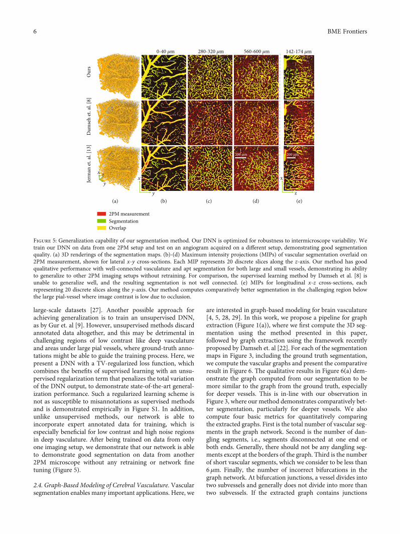
large-scale datasets [27]. Another possible approach forachieving generalization is to train an unsupervised DNN,as by Gur et. al [9]. However, unsupervised methods discardannotated data altogether, and this may be detrimental inchallenging regions of low contrast like deep vasculatureand areas under large pial vessels, where ground-truth anno-tations might be able to guide the training process. Here, wepresent a DNN with a TV-regularized loss function, whichcombines the benefits of supervised learning with an unsu-pervised regularization term that penalizes the total variationof the DNN output, to demonstrate state-of-the-art general-ization performance. Such a regularized learning scheme isnot as susceptible to misannotations as supervised methodsand is demonstrated empirically in Figure S1. In addition,unlike unsupervised methods, our network is able toincorporate expert annotated data for training, which isespecially beneficial for low contrast and high noise regionsin deep vasculature. After being trained on data from onlyone imaging setup, we demonstrate that our network is ableto demonstrate good segmentation on data from another2PM microscope without any retraining or network finetuning (Figure 5).

2.4. Graph-Based Modeling of Cerebral Vasculature. Vascularsegmentation enables many important applications. Here, we

are interested in graph-based modeling for brain vasculature[4, 5, 28, 29]. In this work, we propose a pipeline for graphextraction (Figure 1(a)), where we first compute the 3D seg-mentation using the method presented in this paper,followed by graph extraction using the framework recentlyproposed by Damseh et. al [22]. For each of the segmentationmaps in Figure 3, including the ground truth segmentation,we compute the vascular graphs and present the comparativeresult in Figure 6. The qualitative results in Figure 6(a) dem-onstrate the graph computed from our segmentation to bemore similar to the graph from the ground truth, especiallyfor deeper vessels. This is in-line with our observation inFigure 3, where our method demonstrates comparatively bet-ter segmentation, particularly for deeper vessels. We alsocompute four basic metrics for quantitatively comparingthe extracted graphs. First is the total number of vascular seg-ments in the graph network. Second is the number of dan-gling segments, i.e., segments disconnected at one end orboth ends. Generally, there should not be any dangling seg-ments except at the borders of the graph. Third is the numberof short vascular segments, which we consider to be less than6μm. Finally, the number of incorrect bifurcations in thegraph network. At bifurcation junctions, a vessel divides intotwo subvessels and generally does not divide into more thantwo subvessels. If the extracted graph contains junctions

142-174 𝜇m0-40 𝜇m 280-320 𝜇m 560-600 𝜇m

200 𝜇m 200 𝜇m

y

zx

x

y

x

z

Our

sD

amse

h et

. al.

[8]

Jerm

an et

. al.

[13]

2PM measurement

(a) (b) (c) (d) (e)

SegmentationOverlap

Figure 5: Generalization capability of our segmentation method. Our DNN is optimized for robustness to intermicroscope variability. Wetrain our DNN on data from one 2PM setup and test on an angiogram acquired on a different setup, demonstrating good segmentationquality. (a) 3D renderings of the segmentation maps. (b)-(d) Maximum intensity projections (MIPs) of vascular segmentation overlaid on2PM measurement, shown for lateral x-y cross-sections. Each MIP represents 20 discrete slices along the z-axis. Our method has goodqualitative performance with well-connected vasculature and apt segmentation for both large and small vessels, demonstrating its abilityto generalize to other 2PM imaging setups without retraining. For comparison, the supervised learning method by Damseh et al. [8] isunable to generalize well, and the resulting segmentation is not well connected. (e) MIPs for longitudinal x-z cross-sections, eachrepresenting 20 discrete slices along the y-axis. Our method computes comparatively better segmentation in the challenging region belowthe large pial-vessel where image contrast is low due to occlusion.

6 BME Frontiers

where a vessel divides into three or more subvessels, we con-sider it to be an incorrect bifurcation. We compare these met-rics among the extracted graphs in Figure 6(b) and find thatthe performance of our method resembles most closely to theground truth. We also compute the graphs using the segmen-tation maps from Figure 5 and present the qualitative com-parison in Figure S2, empirically demonstrating satisfactorygraph extraction performance up to a depth of 600μm. Wethus demonstrate that our segmentation method is suitablefor large-scale vascular modeling and subsequent graphextraction.

3. Discussion

We propose and experimentally demonstrate a novel methodfor the segmentation of 2PM angiograms, with the goal oflarge-scale cerebrovascular modeling. This new strategyenables the processing of much larger angiograms comparedto the existing methods with significantly faster computationspeed, by leveraging recent advances in deep learning. Inaddition, our deep neural network is able to segment angio-grams from multiple 2PM imaging systems without retrain-ing, and this flexibility shows its potential to be used as a

40-80 𝜇m 286-326 𝜇m 566-606 𝜇m

Gro

und

trut

hO

urs

Dam

seh

et. a

l. [8

]Je

rman

et. a

l. [1

3]

y

zx

160 𝜇m

x

y

2PM measurement

(I) (II) (III) (IV)

Graph connection

Metrics Total segments Dangling segments Short segments Incorrectbifurcations

Ground truth 3269330919132364

330828938

1060

413375172269

22024315

192

OursDamseh et. al. [8]Jerman et. al. [13]

(a)

(b)

Figure 6: Graph extraction from 3D segmentation. The mathematical graph of the vasculature, comprising of nodes connected via edges, wascomputed from the segmentations in Figure 3. (a) Qualitative comparison of graph extraction performance. (I) 3D view of the graphs depictedas vascular center lines in the volume. (II-IV) MIPs of graphs overlaid on 2PM measurement, each MIP representing 20 discreet slices alongthe z-axis. Graph extraction from our segmentation is qualitatively better compared to other methods, especially at increased depth. (b) Acomparison of metrics demonstrates that the graph computed from our segmentation is quantitatively most similar to the graph from theground truth segmentation.

7BME Frontiers

general 3D segmentation tool for large-scale angiogramsobtained using any 2PM imaging setup. In light of our goalof graph-based modeling of the cerebral vasculature, we com-pute vascular graphs from binary segmentation, using a tech-nique recently developed by one of our co-authors [22]. Weobserve that improved segmentation using our method ledto better vascular graphs for large 2PM angiograms. Thishas important implications since existing graph extractionpipelines do not demonstrate adequate accuracy and haveto be followed up by significant manual correction as a post-processing step [29]. This human annotation can quicklybecome infeasible as the angiograms scale to greater sizesand quantities. It is therefore desirable to have a method foraccurate graph computation which can minimize, if notcompletely eliminate, the use of manual correction. Towardsthis end, we have presented a modular approach for graphcomputation, where the challenging 2PM vascular segmenta-tion has been decoupled from graph extraction. This gives usthe ability to optimize each of these two steps independently.

While our method was able to demonstrate significantlydeeper segmentation compared to existing techniques, it stillhas several limitations. Our method was unable to accuratelysegment vasculature beyond 600μm within the brain tissue.This is partly due to the limitation of 2PM to capture angio-grams with sufficient SBRs much beyond this depth and alsodue to the unavailability of accurate ground truth for deeperangiograms. Effective segmentation for deeper vasculaturemight be achieved by employing ground-truth data withgreater depth, coupled with more intelligent semisupervisedlearning, involving, e.g., active contours [30], in addition tothe TV regularization used in our work. Another limitationis that angiograms from different setups have to undergomanual histogram equalization before being segmented byour network. This involves linear scaling to make the voxeldistribution of new angiograms similar to those on whichthe network has been trained. Further work may look toautomate the process. In general, more advanced domainadaptation techniques [31, 32] may be incorporated to fur-ther improve the generalizability. Although we demonstrateimproved segmentation performance in the low-contrastregion under large pial vessels compared to existing methods,the segmentation still suffers from artifacts and obvious falsenegatives. Further work may look to improve the perfor-mance in such regions, on the acquisition end either byemploying better fluorophores or by using a preprocessingmethod to enhance the contrast of the vasculature under pialvessels, prior to segmentation. Despite these limitations, wedemonstrate state-of-the-art performance for vascular seg-mentation of large-scale 2PM angiograms. We believe thatthis work paves the way towards large-scale cerebrovascularmodeling and analysis.

4. Materials and Method

4.1. Data Preparation. 2PM angiograms were acquired ontwo different imaging systems for various mice specimen(n = 5 for system 1 and n = 1 for system 2). For trainingand quantitative evaluation, we used data only from the firstimaging setup, while data from the second setup was used for

qualitative demonstration of the generalizability of ourapproach.

The dataset from imaging system 1 has been previouslypublished by Gagnon et al. [5, 29], and its preparation isdetailed as follows. All experimental procedures wereapproved by the Massachusetts General Hospital Subcom-mittee on Research Animal Care. C57BL/6 mice (male, 25-30 g, n = 5) were anesthetized by isoflurane (1-2% in a mix-ture of O2 and air) under constant temperature (37°C). A cra-nial window with the dura removed was sealed with a 150mthick microscope cover-slip. During the experiments, a cath-eter was used in the femoral artery to monitor the systemicblood pressure and blood gases and to administer the two-photon dyes. During the measurement period, mice breatheda mixture of O2 and air under the 0.7-1.2% isoflurane anes-thesia. The structural imaging of the cortical vasculaturewas performed using a custom-built two-photon microscope[33] after labeling the blood plasma with dextranconjugatedfluorescein (FITC) at 500nM concentration. Image stacksof the vasculature were acquired with 1:2 × 1:2 × 2:0 μmvoxel sizes under a 20x Olympus objective (NA = 0:95). Datawas digitized with a 16-bit depth. A total of five angiogramswere acquired on this setup, each from a distinct specimenFigure S3(A-E), and were divided into training and testingangiograms in a ratio of 80-20%, respectively, i.e., fourangiograms were used for training (Figure S3(B-E)), whileone was used for testing and evaluation (Figure S3(B-E)).The ground-truth segmentation was prepared by humanannotators using custom software.

For imaging system 2, the dataset has a similar prepara-tion process for the live specimen; however, it was acquiredon a different imaging system and a different mouse whosedetails are as follows. All experimental procedures wereapproved by the BU IACUC. We anesthetized a C57BL/6Jmouse with isoflurane (1–2% in a mixture of O2 and air)under constant temperature (37°C). A cranial window withthe dura intact was sealed with a 150m thick microscopecover-slip. During the measurement period, the micebreathed a mixture of O2 and air under 0.7–1.2% isofluraneanesthesia. The blood plasma was labeled using dextrancon-jugated fluorescein (FITC) at 500nM concentration. Imagingwas performed using a Bruker two-photon microscope usinga 16x objective (NA = 0:8) with voxel size 1:58 × 1:58 × 2:0 μm. Data was digitized with a 12-bit depth. One angiogramwas acquired on this setup (Figure S3(F)) and was used totest the generalization capability of our network.

4.2. Data Preprocessing. Adequate preprocessing on test datawas found to be critical for good network generalization.Here, we present a two-step preprocessing method that con-sists of histogram scaling, followed by noise removal, forimproved segmentation.

Since our two imaging setups have different detector bit-depths, their respective angiograms also differed with respectto the scale of voxel intensities (Figure S4(A, C)). Since ourDNN learns a maximum likelihood function for mappingthe input angiograms to the desired 3D segmentation maps,given the training data, it is important that the testangiogram from any imaging system is on a similar

8 BME Frontiers

intensity scale as the training data. Noticing that thehistograms from both setups are similar in shape(Figure S4(A, C)), but different with respect to intensityscale, we perform linear scaling on data from setup 2 bymultiplying it with a nonnegative scaling factor. The scalingfactor is chosen such that after scaling, the intensityhistogram of the angiogram from setup 2 becomes similarin scale to the intensity histogram of the angiogram fromsetup 1. This procedure has been depicted in Figure S4(B,D). The scaling factor for our case was empirically chosento be 16. In the case of applying this approach to anangiogram from a different imaging setup, the procedurewill be very similar. This new angiogram would have to bemultiplied with a nonnegative scaling factor, which isempirically chosen such that the voxel-intensity histogramof the scaled angiogram becomes similar in scale to that ofan angiogram from setup 1.

A well-known challenge inherent to 2PM is the degrada-tion of signal with imaging depth (Figure 2, Figure S5(A)).Segmentation on such an angiogram using our trainedDNN has significant artifacts, even after linear scaling.Here, we propose a simple yet effective method to reducethis depth-dependent noise. We subtracted from each 2Dimage in a 2PM 3D stack its median value. This visiblyimproved the signal quality by suppressing the backgroundnoise, especially in deeper layers (Figure S5(B)). Theangiogram was further improved by applying a 3D medianfilter with a kernel of size 3 voxels (Figure S5(C)). Thispreprocessing method improved the segmentation of thedeep vasculature and made individual vessels moredistinguishable (Figure S6). However, this method wasobserved to decrease segmentation quality in the shadowedregion under large pial vessels where the measurementcontrast is comparatively weak. A locally adaptivepreprocessing method that could overcome this limitationmay be a potential direction of future work.

4.3. Deep Neural Network Design and Implementation. OurDNN architecture is based on the well-known V-net [34];however, we significantly modified the original frameworkfor large-scale 2PM vascular segmentation (Figure S7). Thenetwork is end-to-end 3D for fast computation, as opposedto 2D slice-wise techniques, and consequently also takesinto account the 3D context for improved segmentation. Ithas an encoder-decoder framework for learning vascularfeatures at various size scales and high-resolution featureforwarding to retain high-frequency information. Weincorporate batch normalization after each convolutionlayer to improve generalization performance andconvergence speed. Our network processes 3D inputpatches with outputs of the same size. Patch-basedprocessing enables the segmentation of arbitrarily largevolumes. Our large patch size compared to the existingmethods, coupled with a lightweight network, helps tosignificantly accelerate the computation speed. For thetraining process, the training data is divided into patches of128 × 128 × 128 voxels, with an overlap of 64 voxels alongall axes. Each training iteration processes a batch of 4patches chosen randomly from the training data. We use

Adam optimizer to train our network with a learning rateof 10-4 for about 100 epochs, which takes approximately 4hours on a TitanXp GPU. For testing, the angiogram isdivided into patches of 128 × 128 × 128 voxels, andsegmentation is performed on each patch separately, afterwhich they are stitched together to get the final segmentedangiogram. The division of the acquired data into trainingand testing datasets is described in Section 4.1.

4.4. Loss Function Design. During the training process of aDNN, a loss function is optimized via gradient descent orany of its variants. The loss itself is a function of the networkoutput and is chosen by the user to impart desired character-istics to the DNN output by guiding the training process. Inthis problem, we initially experimented with binary cross-entropy (BCE) loss, as it is known to promote sparsity inthe output [35], which is desirable for vascular segmentation.However, severe class imbalance in our data rendered BCEineffective as a loss function, and the DNN converged to anearly zero solution, i.e., almost all voxels were classified asbackground. Class imbalance is the situation when one classsignificantly outnumbers the others in the training data,causing a preferential treatment by the learning algorithmtowards the abundant class. In our case, the negative classconsisting of background voxels was significantly moreabundant than the positive class and constituted 96% of thetotal voxels in the training data. This resulted in a significantnumber of false negatives in the DNN predictions using BCE.In order to overcome this challenge, we incorporated a vari-ant of BCE loss with a class balancing [36], E, defined as

E Wð Þ = −β〠iϵY+

log P yi = 1 ∣ X ;Wð Þ

− 1 − βð Þ〠iϵY−

log P yi = 0 ∣ X ;Wð Þ,ð1Þ

where P is the probability of obtaining the label yi for the ith

voxel, given data X and network weightsW. β and ð1 − βÞ arethe class weighting multipliers, defined as β = jY−j/jY j, ð1 −βÞ = jY+j/jY j, where Y+ is the set of positive (vessel) labels,Y− is the set of negative (background tissue) labels, and Ybeing the set of all voxels, both vessel and background. In thisloss, we essentially weigh down the negative class and give agreater weight to the positive class, and the assigned weightdepends on the fractions of the vessel and background voxelsin the volume, respectively. Note that β is not a tunablehyperparameter here, rather its value is determined by thetraining data in every iteration. This balanced BCE loss sig-nificantly improved the training in the presence of severeclass imbalance.

Merely using the balanced BCE loss described above wasfound to be insufficient to provide satisfactory generalizationperformance. One way to improve the generalizability is touse training data from various different imaging setups.However, manually annotating many large-scale angiogramsfor this purpose would have been prohibitive due to the asso-ciated time and cost. We therefore took a different approachand employed TV regularization in the loss function, which

9BME Frontiers

improved the generalization in the presence of limited andnoisy training data. For this purpose, we added a regulariza-tion term to the loss function, which penalizes the total vari-ation of the network output. Such a loss based on 2D-TV hasbeen demonstrated by Javanmardi et al. in their preprint[37]. We employ a 3D-TV loss, TV , which is defined as

TV Wð Þ =〠iϵY

∇XP yi ;Wð Þj j + ∇YP yi ;Wð Þj j + ∇ZP yi ;Wð Þj j,

ð2Þ

where ∇X , ∇Y , and ∇Z are 3D Sobel operators for computingTV [38]. TV when added to the balanced BCE loss decreasesthe model dependence on the ground truth data, helping gen-eralization. TV is known to promote sparsity and piece-wisecontinuity in solutions, which are suitable priors to vascularsegmentation. The addition of TV imparted denoising prop-erty to the network, such that no postprocessing was requiredon the outputs after segmentation, and improved the gener-alization performance (Figure Figure S8).

Finally, we also regularize our loss function by adding apenalty on the l2-norm of the network weights W. This iscalled weight decay and is known to encourage the networkto learn smooth mappings from the input angiogram to theoutput segmentations, reducing overfitting and improvinggeneralization. The final form of our loss function L is thus

L Wð Þ = E Wð Þ + αTV Wð Þ + γ Wk kl2 , ð3Þ

where α and γ are tunable parameters, whose values wereempirically found to be 5 × 10−9 and 0.01, respectively, forbest performance. We present how different levels of TV reg-ularization impact the segmentation performance inFigure S9 and demonstrate the range for the optimal valueof α. Similarly, we also show segmentation performance asa function of γ and present the optimal range for weightdecay in Figure S10.

4.5. Segmentation Evaluation Metrics. Accuracy = TP + TN/ðTP + TN + FP + FNÞ, Jaccard index = TP/ðTP + FP + FNÞ,Dice coefficient = 2TP/ð2TP + FP + FNÞ, Specificity = TN/ðFP + TNÞ, and Sensitivity = TP/ðTP + FNÞ. Here, TP (TruePositive) is the number of correctly classified vessel voxels, TN(True Negative) is the number of correctly classified back-ground voxels, FP (False Positive) is the number of backgroundvoxels incorrectly labeled as vessels, and FN (False Negative) isthe number of vessel voxels incorrectly labeled as background.

MCC = TP × TN − FP × FN/ffiffiffiffiffiffiffiffiffiffiffiffiffiffiffiffiffiffiffiffiffiffiffiffiffiffiffiffiffiffiffiffiffiffiffiffiffiffiffiffiffiffiffiffiffiffiffiffiffiffiffiffiffiffiffiffiffiffiffiffiffiffiffiffiffiffiffiffiffiffiffiffiffiffiffiffiffiffiffiffiffiðTP + FPÞðTP + FNÞðTN + FPÞðTN + FNÞp

,which measures the linear correlation between the groundtruth and predicted labels and is a special case of the Pearsoncorrelation coefficient.

HD among two finite point sets can be defined asHDðA, BÞ =max ðhðA, BÞ, hðB, AÞÞ, where hðA, BÞ =max

aϵAminbϵB

ka − bk, k:k being any norm, e.g., Euclidean norm.

LC is defined as LCðS, SGÞ = #ððgðSÞ ∩ SGÞ ∪ ðS ∩ gðSGÞÞÞ/#ðgðSÞ ∪ gðSGÞÞ, where S and SG are the predicted andground truth segmentation, respectively; gð:Þ is an operatorthat computes the 3D vascular skeleton from an input seg-

mentation in the form of a graph of nodes and edges, usingthe method in [22]; and #ð:Þ measures the cardinality of aninput set in terms of the number of voxels.

Conflicts of Interest

The authors declare that they have no competing interests.

Authors’ Contributions

W.T. developed and implemented the software for segmenta-tion and wrote the paper. S.K. helped with the data prepara-tion, deep learning design, and paper writing and performedresults analysis. J.Z. contributed to deep neural networkdesign and implementation. F.T. performed ground-truthannotation. X.C. contributed to experimental design, resultsanalysis, and paper writing. B.S.L. performed data acquisitionon setup 2. A.S. implemented the graph extraction algorithmon the BU cluster. R.D. developed graph extraction softwareand helped with its implementation. F.L. supervised thegraph extraction from vascular segmentation. S.S. helpedwith the experimental design and analysis of data from setup1. D.B. and L.T. initiated, supervised, and coordinated thestudy and help write the manuscript.

Acknowledgments

We thank David Kleinfeld (UCSD), TimothyW. Secomb (Uni-versity of Arizona), Chris B. Schaffer (Cornell University), andNozomiNishimura (Cornell University) for helpful discussions;Yujia Xue (Boston University) and Yunzhe Li (Boston Univer-sity) for the help in running experimental code; and Alex Mat-lock (Boston University) for reviewing the manuscript. Thiswork was supported by NIH 3R01EB021018-04S2.

Supplementary Materials

Figure S1: Robustness of the proposed learning scheme to labelnoise. Figure S2: Graph extraction from the 3D segmentationmap. Figure S3: Training and testing data used in our experi-mentation. Figure S4: Data preprocessing: intensity scaling. Fig-ure S5: Data preprocessing: denoising. Figure S6: Effect ofdifferent steps of preprocessing on segmentation quality. FigureS7: Deep neural network architecture. Figure S8: Ablation of TVand preprocessing for segmentation. Figure S9: Effect of totalvariation (TV) regularization on the segmentation perfor-mance. Figure S10: Effect of L2 regularization (weight decay)on the segmentation performance. (Supplementary Materials)

References

[1] A. Parpaleix, Y. G. Houssen, and S. Charpak, “Imaging localneuronal activity by monitoring PO2 transients in capillaries,”Nature Medicine, vol. 19, no. 2, pp. 241–246, 2013.

[2] K. Kisler, A. R. Nelson, A. Montagne, and B. V. Zlokovic,“Cerebral blood flow regulation and neurovascular dysfunc-tion in Alzheimer disease,” Nature Reviews Neuroscience,vol. 18, no. 7, pp. 419–434, 2017.

[3] P. S. Ozbay, G. Warnock, C. Rossi et al., “Probing neuronalactivation by functional quantitative susceptibility mapping

10 BME Frontiers

under a visual paradigm: a group level comparison with BOLDfMRI and PET,” NeuroImage, vol. 137, pp. 52–60, 2016.

[4] D. A. Boas, S. R. Jones, A. Devor, T. J. Huppert, and A. M.Dale, “A vascular anatomical network model of the spatio-temporal response to brain activation,” NeuroImage, vol. 40,no. 3, pp. 1116–1129, 2008.

[5] L. Gagnon, S. Sakadzic, F. Lesage et al., “Validation and opti-mization of hypercapnic-calibrated fMRI from oxygen-sensitive two-photon microscopy,” Philosophical Transactionsof the Royal Society B: Biological Sciences, vol. 371, no. 1705,article 20150359, 2016.

[6] M. G. Báez-Yánez, P. Ehses, C. Mirkes, P. S. Tsai, D. Kleinfeld,and K. Scheffler, “The impact of vessel size, orientation andintravascular contribution on the neurovascular fingerprintof BOLD bSSFP fMRI,”NeuroImage, vol. 163, pp. 13–23, 2017.

[7] X. Cheng, A. J. L. Berman, J. R. Polimeni et al., “Dependence ofthe MR signal on the magnetic susceptibility of blood studiedwith models based on real microvascular networks,”MagneticResonance in Medicine, vol. 81, no. 6, pp. 3865–3874, 2019.

[8] R. Damseh, P. Pouliot, L. Gagnon et al., “Automatic graph-based modeling of brain microvessels captured with two-photon microscopy,” IEEE Journal of Biomedical and HealthInformatics, vol. 23, no. 6, pp. 2551–2562, 2019.

[9] S. Gur, L. Wolf, L. Golgher, and P. Blinder, “Unsupervisedmicrovascular image segmentation using an active contoursmimicking neural network,” in 2019 IEEE/CVF InternationalConference on Computer Vision (ICCV), pp. 10722–10731,Seoul, Korea (South), October-November 2019.

[10] M. Haft-Javaherian, L. Fang, V. Muse, C. B. Schaffer,N. Nishimura, andM. R. Sabuncu, “Deep convolutional neuralnetworks for segmenting 3d in vivo multiphoton images ofvasculature in Alzheimer disease mouse models,” PLoS One,vol. 14, no. 3, article e0213539, 2019.

[11] F. Helmchen and W. Denk, “Deep tissue two-photon micros-copy,” Nature Methods, vol. 2, no. 12, pp. 932–940, 2005.

[12] A. F. Frangi, W. J. Niessen, K. L. Vincken, andM. A. Viergever,“Multiscale vessel enhancement filtering,” in Medical ImageComputing and Computer-Assisted Intervention — MIC-CAI’98. MICCAI 1998. Lecture Notes in Computer Science,vol 1496, W. M. Wells, A. Colchester, and S. Delp, Eds.,pp. 130–137, Springer Berlin Heidelberg, Berlin, Heidelberg,1998.

[13] T. Jerman, F. Pernus, B. Likar, and Z. Spiclin, “Enhancement ofvascular structures in 3D and 2D angiographic images,” IEEETransactions on Medical Imaging, vol. 35, no. 9, pp. 2107–2118, 2016.

[14] K. Poon, G. Hamarneh, and R. Abugharbieh, “Live-vessel:extending livewire for simultaneous extraction of optimalmedial and boundary paths in vascular images,” in MedicalImage Computing and Computer-Assisted Intervention –MIC-CAI 2007. MICCAI 2007. Lecture Notes in Computer Science,vol 4792, N. Ayache, S. Ourselin, and A. Maeder, Eds.,pp. 444–451, Springer, Berlin, Heidelberg, 2007.

[15] M. W. Law and A. C. Chung, “Three dimensional curvilinearstructure detection using optimally oriented flux,” in Com-puter Vision – ECCV 2008. ECCV 2008. Lecture Notes in Com-puter Science, vol 5305, D. Forsyth, P. Torr, and A. Zisserman,Eds., pp. 368–382, Springer, Berlin, Heidelberg, 2008.

[16] A. Vasilevskiy and K. Siddiqi, “Flux maximizing geometricflows,” IEEE Transactions on Pattern Analysis and MachineIntelligence, vol. 24, no. 12, pp. 1565–1578, 2002.

[17] P. Teikari, M. Santos, C. Poon, and K. Hynynen, “Deeplearning convolutional networks for multiphoton micros-copy vasculature segmentation,” 2016, http://arxiv.org/abs/1606.02382.

[18] S. Jégou, M. Drozdzal, D. Vazquez, A. Romero, and Y. Bengio,“The one hundred layers tiramisu: fully convolutional dense-nets for semantic segmentation,” in 2017 IEEE Conference onComputer Vision and Pattern Recognition Workshops(CVPRW), pp. 11–19, Honolulu, HI, USA, July 2017.

[19] S. Niu, Q. Chen, L. De Sisternes, Z. Ji, Z. Zhou, and D. L.Rubin, “Robust noise region-based active contour model vialocal similarity factor for image segmentation,” Pattern Recog-nition, vol. 61, pp. 104–119, 2017.

[20] K. Weiss, T. M. Khoshgoftaar, and D. Wang, “A survey oftransfer learning,” Journal of Big Data, vol. 3, no. 1, p. 9, 2016.

[21] M. Ghafoorian, A. Mehrtash, T. Kapur et al., “Medical ImageComputing and Computer Assisted Intervention − MICCAI2017,” in Medical Image Computing and Computer AssistedIntervention − MICCAI 2017. MICCAI 2017. Lecture Notes inComputer Science, vol 10435, M. Descoteaux, L. Maier-Hein,A. Franz, P. Jannin, D. Collins, and S. Duchesne, Eds.,pp. 516–524, Springer, Cham, 2017.

[22] R. Damseh, P. Delafontaine-Martel, P. Pouliot, F. Cheriet, andF. Lesage, “Laplacian flow dynamics on geometric graphs foranatomical modeling of cerebrovascular networks,” IEEETransactions on Medical Imaging, vol. 39, p. 1, 2020.

[23] A. A. Taha and A. Hanbury, “Metrics for evaluating 3d medi-cal image segmentation: analysis, selection, and tool,” BMCMedical Imaging, vol. 15, no. 1, p. 29, 2015.

[24] A. Lahiri, A. G. Roy, D. Sheet, and P. K. Biswas, “Deep neuralensemble for retinal vessel segmentation in fundus imagestowards achieving label-free angiography,” in 2016 38thAnnual International Conference of the IEEE Engineering inMedicine and Biology Society (EMBC), pp. 1340–1343,Orlando, FL, USA, August 2016.

[25] S. Boughorbel, F. Jarray, and M. El-Anbari, “Optimal classifierfor imbalanced data using Matthews correlation coefficientmetric,” PLoS One, vol. 12, no. 6, article e0177678, 2017.

[26] M. E. Gegundez-Arias, A. Aquino, J. M. Bravo, and D. Marin,“A function for quality evaluation of retinal vessel segmenta-tions,” IEEE Transactions on Medical Imaging, vol. 31, no. 2,pp. 231–239, 2012.

[27] J. Han, P. Luo, and X. Wang, “Deep self-learning from noisylabels,” in 2019 IEEE/CVF International Conference on Com-puter Vision (ICCV), pp. 5138–5147, Seoul, Korea (South),October-November 2019.

[28] L. Gagnon, A. F. Smith, D. A. Boas, A. Devor, T. W. Secomb,and S. Sakadzic, “Modeling of cerebral oxygen transport basedon in vivo microscopic imaging of microvascular networkstructure, blood flow, and oxygenation,” Frontiers in Compu-tational Neuroscience, vol. 10, p. 82, 2016.

[29] L. Gagnon, S. Sakad i, F. Lesage et al., “Quantifying the micro-vascular origin of BOLD-fMRI from first principles with two-photon microscopy and an oxygen-sensitive nanoprobe,”Journal of Neuroscience, vol. 35, no. 8, pp. 3663–3675, 2015.

[30] D. Marcos, D. Tuia, B. Kellenberger et al., “Learning deepstructured active contours end-to-end,” in 2018 IEEE/CVFConference on Computer Vision and Pattern Recognition,pp. 8877–8885, Salt Lake City, UT, USA, June 2018.

[31] H. Venkateswara, S. Chakraborty, and S. Panchanathan,“Deep-learning systems for domain adaptation in computer

11BME Frontiers

vision: learning transferable feature representations,” IEEE Sig-nal Processing Magazine, vol. 34, no. 6, pp. 117–129, 2017.

[32] K. Kamnitsas, C. Baumgartner, C. Ledig et al., “Unsuperviseddomain adaptation in brain lesion segmentation with adver-sarial networks,” in Lecture Notes in Computer Science, M.Niethammer, Ed., vol. 10265, pp. 597–609, Springer, 2017.

[33] S. Sakadžić, E. Roussakis, M. A. Yaseen et al., “Two-photonhigh-resolution measurement of partial pressure of oxygen incerebral vasculature and tissue,” Nature Methods, vol. 7,no. 9, pp. 755–759, 2010.

[34] F. Milletari, N. Navab, and S.-A. Ahmadi, “V-net: fully convo-lutional neural networks for volumetric medical image seg-mentation,” in 2016 Fourth International Conference on 3DVision (3DV), pp. 565–571, Stanford, CA, USA, October 2016.

[35] Y. Li, Y. Xue, and L. Tian, “Deep speckle correlation: a deeplearning approach toward scalable imaging through scatteringmedia,” Optica, vol. 5, no. 10, pp. 1181–1190, 2018.

[36] S. Xie and Z. Tu, “Holistically-nested edge detection,” in 2015IEEE International Conference on Computer Vision (ICCV),pp. 1395–1403, Santiago, Chile, December 2015.

[37] M. Javanmardi, M. Sajjadi, T. Liu, and T. Tasdizen, “Unsuper-vised total variation loss for semi supervised deep learning ofsemantic segmentation,” 2016, http://arxiv.org/abs/1605.01368.

[38] A. A. Aqrawi, T. H. Boe, and S. Barros, “Detecting salt domesusing a dip guided 3D Sobel seismic attribute,” in SEG Techni-cal Program Expanded Abstracts 20sssss11, pp. 1014–1018,Society of Exploration Geophysicists, 2011.

12 BME Frontiers