Anatomy: Simple and Effective Privacy Preservation - Department of

Anatomy: Simple and Effective Privacy Preservation

Xiaokui Xiao Yufei TaoDepartment of Computer Science and Engineering

Chinese University of Hong KongSha Tin, New Territories, Hong Kong{xkxiao, taoyf}@cse.cuhk.edu.hk

ABSTRACTThis paper presents a novel technique,anatomy, for publishing sen-sitive data. Anatomy releases all the quasi-identifier and sensitivevalues directly in two separate tables. Combined with a groupingmechanism, this approach protects privacy, and captures a largeamount of correlation in the microdata. We develop a linear-timealgorithm for computing anatomized tables that obey thel-diversityprivacy requirement, and minimize the error of reconstructing themicrodata. Extensive experiments confirm that our technique al-lows significantly more effective data analysis than the conven-tional publication method based on generalization. Specifically,anatomy permits aggregate reasoning with average error below10%, which is lower than the error obtained from a generalizedtable by orders of magnitude.

1. INTRODUCTIONPrivacy preservation is a serious concern in publication ofpersonaldata. Using a popular example in the literature, assume thata hos-pital wants to release patients’ medical records in Table 1,referredto as themicrodata. AttributeDiseaseis sensitive, that is, the hos-pital must ensure that no adversary can correctly infer the diseaseof any patient with significant confidence.Age, Sex, andZipcodeare thequasi-identifier(QI) attributes, because they may be uti-lized in combination to reveal the identity of an individual, leadingto privacy breach.

Consider an adversary who has the personal details (i.e., age 23 andzipcode 11000) of Bob, and knows that Bob has been hospitalizedbefore. In Table 1, since only tuple 1 matches Bob’s QI-values, theadversary asserts that Bob contracted pneumonia.

To avoid this problem,generalization[12, 13, 14, 10] divides tuplesinto QI-groups, and transforms their QI-values into less specificforms, so that tuples in the same QI-group cannot be distinguishedby their QI-values. Table 2 is a generalized version of Table1 (e.g.,the age 23 and zipcode 11000 of tuple 1 have been replaced withintervals[21, 60] and[10001, 60000], respectively). Here, general-ization produces two QI-groups, including tuples 1-4 and 5-8, re-spectively. As a result, even if an adversary has the exact QIvalues

Permission to copy without fee all or part of this material isgranted providedthat the copies are not made or distributed for direct commercial advantage,the VLDB copyright notice and the title of the publication and its date appear,and notice is given that copying is by permission of the Very Large DataBase Endowment. To copy otherwise, or to republish, to post on serversor to redistribute to lists, requires a fee and/or special permission from thepublisher, ACM.VLDB ‘06,September 12-15, 2006, Seoul, Korea.Copyright 2006 VLDB Endowment, ACM 1-59593-385-9/06/09

tuple ID Age Sex Zipcode Disease1 (Bob) 23 M 11000 pneumonia

2 27 M 13000 dyspepsia3 35 M 59000 dyspepsia4 59 M 12000 pneumonia5 61 F 54000 flu6 65 F 25000 gastritis

7 (Alice) 65 F 25000 flu8 70 F 30000 bronchitis

Table 1: The microdatatuple ID Age Sex Zipcode Disease

1 [21, 60] M [10001, 60000] pneumonia2 [21, 60] M [10001, 60000] dyspepsia3 [21, 60] M [10001, 60000] dyspepsia4 [21, 60] M [10001, 60000] pneumonia5 [61, 70] F [10001, 60000] flu6 [61, 70] F [10001, 60000] gastritis7 [61, 70] F [10001, 60000] flu8 [61, 70] F [10001, 60000] bronchitis

Table 2: A 2-diverse table

of Bob, s/he still does not know which tuple in the first QI-groupbelongs to Bob.

Two notions,k-anonymityand l-diversity, have been proposed tomeasure the degree of privacy preservation. A (generalized) tableis k-anonymous[12, 13, 14] if each QI-group involves at leastktuples (e.g., Table 2 is 4-anonymous). However, as shown in [10],even with a largek, k-anonymity may still allow an adversary toinfer the sensitive value of an individual with extremely high con-fidence. Hence, we adoptl-diversity [10], which provides strongerprivacy protection.

Specifically, a table isl-diverse if, in each QI-group, at most1/l ofthe tuples possess the most frequent sensitive value1. For instance,Table 2 is2-diverse because, in each QI-group, at most 50% ofthe tuples have the sameDiseasevalue. As mentioned earlier, theadversary (targeting Bob’s medical record) knows that Bob’s tuplemust be in the first QI-group, where two tuples are associatedwithpneumonia, and two with dyspepsia. Hence, the adversary canonlymake a probabilistic conjecture: Bob could have contractedeitherdisease with the same probability.

1.1 Defects of Generalization in AggregateAnalysis

Although generalization preserves privacy, it often losesconsid-erable information in the microdata, which severely compromises1l-diversity has more complicated requirements, if an adversary’s“background knowledge” is taken into account [10]. We will dis-cuss this issue in Section 3.1.

139

��

��

��

��

��

��

��

��

��

��

� �

�

�

��

�

��

Figure 1: The original and generalized data in theAge-Zipcodeplane

the accuracy of data analysis. Assume that the hospital releasesTable 2, and that a researcher wants to derive from this tableanestimate for the following query:

A: SELECT COUNT(*) FROM Unknown-MicrodataWHERE Disease= ‘pneumonia’ AND Age<= 30

AND ZipcodeIN [10001, 20000]

To illustrate how to process the query, Figure 1 shows a 2D space,where the x-, y-dimensions areAgeandZipcode, respectively. Eachpoint denotes a tuple in the microdata of Table 1. For example, thex-, y-coordinates of point 1 equal the age and zipcode of tuple 1,respectively. RectangleR1 (orR2) is obtained from the generalizedvalues in the first (or second) QI-group in Table 2. For instance,the x- (y-) projection ofR1 is the generalized age[20, 60] (zipcode[10001, 60000]) of tuples 1-4. Query A is represented as the shadedrectangleQ, whose projection on the x- (y-) dimension is decidedby the range conditionAge≤ 30 (10001 ≤ Zipcode≤ 20000).

Since the researcher sees onlyR1 andR2 (but not the points), s/heanswers query A in a way similar to selectivity estimation onamultidimensional histogram [15], as suggested in [9]. Clearly, asR2 is disjoint withQ, no tuple in the second QI-group can satisfythe query. R1, however, intersectsQ, and hence, is examined asfollows.

From theDisease-values in Table 2, the researcher knows that 2 tu-ples in the first QI-group are associated with pneumonia. It remainsto calculate the probabilityp that a tuple in the QI-group qualifiesthe range predicates of A, or equivalently, the tuple’s point rep-resentation falls inQ (Figure 1). Oncep is available, the queryanswer can be estimated as2p.

Without additional knowledge, the researcher assumes uni-form data distribution inR1, and computesp as Area(R1 ∩RQ)/Area(R1) = 0.05. This value leads to an approximate an-swer 0.1, which, however, is ten times smaller than actual queryresult 1 (see Table 1).

The gross error is caused by the fact that the data distribution inR1

significantly deviates from uniformity. Nevertheless, given onlythe generalized table, we cannot justify any other distribution as-sumption. This is an inherent problem of generalization: itpreventsan analyst from correctly understanding the data distribution insideeach QI-group.

1.2 Rationale of AnatomyTo overcome the defects of generalization, we propose an innova-tive technique,anatomy, to achieve privacy-preserving publicationthat captures the exact QI-distribution.

Specifically, anatomy releases aquasi-identifier table(QIT) and a

row # Age Sex Zipcode Group-ID1 23 M 11000 12 27 M 13000 13 35 M 59000 14 59 M 12000 15 61 F 54000 26 65 F 25000 27 65 F 25000 28 70 F 30000 2

(a) The quasi-identifier table (QIT)

Group-ID Disease Count1 dyspepsia 21 pneumonia 22 bronchitis 12 flu 22 gastritis 1

(b) The sensitive table (ST)

Table 3: The anatomized tables

sensitive table(ST), which separate QI-values from sensitive val-ues. For example, Tables 3a and 3b demonstrate the QIT and STobtained from the microdata Table 1, respectively.

Construction of the anatomized tables can be (informally) under-stood as follows. First, we partition the tuples of the microdata intoseveral QI-groups, based on a certain strategy. Here, following thegrouping in Table 2, let us place tuples 1-4 (or 5-8) of Table 1intoQI-group 1 (or 2).

Then, we create the QIT. Specifically, for each tuple in Table1, theQIT (Table 3a) includes all itsexactQI-values, together with itsgroup membership in a new columnGroup-ID. However, QIT doesnot store anyDiseasevalue.

Finally, we produce the ST (Table 3b), which retains theDiseasestatistics of each QI-group. For instance, the first two records ofthe ST (to avoid confusion, we use ‘record’, instead of ‘tuple’, forthe data of an ST) indicate that, two tuples of the first QI-groupare associated with dyspepsia, and two with pneumonia. Similarly,the next three records imply that, the second QI-group has a tupleassociated with bronchitis, two with flu, and one with gastritis.

Anatomy preserves privacy because the QIT does not indicatethesensitive value of any tuple, which must be randomly guessedfromthe ST. To explain this, consider again the adversary who hastheage 23 and zipcode 11000 of Bob. Hence, from the QIT (Table 3a),the adversary knows that tuple 1 belongs to Bob, but does not ob-tain any information about his disease so far. Instead, s/hegets theid 1 of the QI-group containing tuple 1. Judging from the ST (Ta-ble 3b), the adversary realizes that, among the 4 tuples in QI-group1, 50% of them are associated with dyspepsia (or pneumonia) inthe microdata. Note that s/he does not gain any additional hints,regarding the exact diseases carried by these tuples. Hence, s/hearrives at the conclusion that Bob could have contracted dyspepsia(or pneumonia) with 50% probability. This is the same conjectureobtainable from the generalized Table 2, as mentioned earlier.

By announcing the QI values directly, anatomy permits more effec-tive analysis than generalization. Given query A in Section1.1, weknow, from the ST (Table 3b), that 2 tuples carry pneumonia inthemicrodata, and they are both in QI-group 1. Hence, we proceedtocalculate the probabilityp that a tuple in the QI-group falls inQ(Figure 1). This calculation does not need any assumption aboutthe data distribution in theAge-Zipcodeplane,because the distrib-

140

ution is precisely released. Specifically, the QIT (Table 3a) showsthat tuples 1 and 2 in QI-group 1 appear inQ, leading to theexactp = 50%. Thus, we obtain an answer2p = 1, which is also theactual query result.

1.3 ContributionsThis paper presents a systematic study of the anatomy technique.First, we formalize the new methodology, based on the privacy re-quirement ofl-diversity. Every pair of QIT and ST ensures that thesensitive value of any individual involved in the microdatacan becorrectly inferred by an adversary with probability at most1/l. Alargerl leads to stronger privacy protection.

Second, we clarify the theoretical reasoning behind the superiorityof anatomy in capturing data correlation. Our results show thatanatomy permits a more accurate modeling of each tuple in themicrodata than generalization. We provide detailed analysis of themodeling error, and quantify it into a closed formula.

Third, we develop an algorithm that computes anatomized tablesin O(n/b) I/Os, wheren is the cardinality of the microdata, andb the page size. These tables have provably good quality guaran-tee, achieving a modeling error deviating from the theoretical lowerbound by a factor of at most1+1/n. Notice that,n is very large inpractice (e.g., at the order a million); hence, our algorithm is nearlyoptimal.

Finally, we prove, through extensive experiments, that anatomysignificantly outperforms generalization, in botheffectiveness ofdata analysisandcomputation cost. Specifically, the anatomizedtables permit highly accurate aggregate search (e.g., query A inSection 1), with average error below 10%, which is lower thanthe query error obtained from a generalized table by orders ofmagnitude. The query accuracy of anatomy is unaffected by thedataset dimensionality, whereas the accuracy of generalization de-cays severely as dimensionality increases. Furthermore, anato-mized tables can be computed much faster than generalized tables.

The rest of the paper is organized as follows. Section 2 surveys theprevious work on generalization. Section 3 formalizes the anatomymethodology, and clarifies its privacy protection guarantees. Sec-tion 4 analyzes correlation preservation. Section 5 develops an al-gorithm for computing anatomized tables. Section 6 experimen-tally evaluates the proposed solutions. Section 7 concludes the pa-per with directions for future work.

2. RELATED WORKGeneralization has been very well studied in the literature[1, 2, 4,5, 6, 7, 8, 9, 10, 11, 12, 13, 14, 16, 17, 18]. LeFevre et al. [8] presentan interesting taxonomy to categorize alternative methodsbased ontheir “encoding schemes”, which impose different constraints ingeneralizing a QI-value. The highest level of the taxonomy dis-tinguishesglobal recodingfrom local recoding. Specifically, theformer requires that, all the tuples with equivalent QI-values mustbe included in the same QI-group. For instance, tuples 6 and 7inTable 1 have identical QI-values; hence, they both appear inthesecond QI-group of Table 2. Local recoding removes this require-ment, but has not received considerable attention in the literature(currently, this approach is applied only in several “suppression-based” solutions [8]).

The category of global recoding can be further divided intoSingle-dimension encodingandmultidimension encoding. Specifically, an

encoding is single dimensional, if the generalized forms oftwo ar-bitrary QI-groups on the same attribute are either disjointor equiv-alent, as is the case in Table 2. When the condition is not sat-isfied, the encoding is multidimensional. For example, imaginethat theZipcode-values of tuples 5-8 in Table 2 were changed to[20001, 60000], which intersects but is not identical to theZipcode-form of tuples 1-4; as a result, the generalization would becomemultidimensional.

Computing the optimal generalization is harder for encodingschemes with fewer constraints. Unfortunately, it is NP-hard tofind the optimal solution, even for simple schemes and quality met-rics [2, 9, 11]. Therefore, the existing algorithms rely on heuristicsfor pruning the search space, in order to discover reasonable gener-alization within a time limit.

A majority of the literature focuses onk-anonymous general-ization. However, Machanavajjhala et al. [10] observe thatk-anonymity fails to secure privacy in practice. In particular, theyshow that, the degree of privacy protection does not really dependon the size of a QI-group, but instead, is determined by the numberof distinctsensitive values in each QI-group. The observation leadsto l-diversity (as will be formalized in Section 3). The analysisof [17] proves thatl-diversity always guarantees stronger privacypreservation thank-anonymity.

A serious drawback of generalization is that, when the number d ofQI attributes is large, any generalization necessarily loses consider-able information in the microdata [1], due to the “curse of dimen-sionality”. Specifically, in high dimensional spaces, eachgeneral-ized value is always an exceedingly wide interval, in which casethe published table is simply useless for research.

This paper is virtually orthogonal to all the previous work.Theproposed anatomy technique is a brand-new approach for publish-ing personal data, which remedies the defects of generalization.Specifically, nearly-optimal anatomized tables can be computed inlinear-time with respect to the database cardinality, and capture asignificant amount of correlation for any dimensionality.

3. FORMALIZATION OF ANATOMYLet T be the microdata that needs to be published.T containsdquasi-identifier (QI) attributesAqi

1 , Aqi2 , ..., Aqi

d , and a sensitiveattributeAs. EachAqi

i (1 ≤ i ≤ d) can be either numerical orcategorical, butAs should be categorical, following the assumptionof l-diversity [10]. For any tuplet ∈ T , we denotet[i] (1 ≤ i ≤ d)as theAqi

i value of t, andt[d + 1] as itsAs value. As a result,t can be regarded as a point in a(d + 1)-dimensional data space,denoted asDS. In Section 3.1, we first clarify the relevant conceptsof anatomy. Then, Section 3.2 explains the privacy guarantees ofanatomized tables.

3.1 ConceptsAs with generalization, Anatomy requires partitioning themicro-dataT .

DEFINITION 1. (Partition/QI-group) A partition consists ofseveral subsets ofT , such that each tuple inT belongs to exactlyone subset. We refer to these subsets asQI-groups, and denotethem asQI1, QI2, ...,QIm. Namely,

�mj=1 QIj = T and, for any

1 ≤ j1 6= j2 ≤ m, QIj1 ∩ QIj2 = ∅.

141

We are interested only inl-diverse partitions that can lead to prov-ably good privacy guarantees:

DEFINITION 2. (l-diverse partition [10]) A partition with mQI-groups isl-diverse, if each QI-groupQIj (1 ≤ j ≤ m) satisfiesthe following condition. Letv be the most frequentAs value inQIj , andcj(v) the number of tuplest ∈ QIj with t[d + 1] = v;then

cj(v)/|QIj | ≤ 1/l (1)

where|QIj | is the size (the number of tuples) ofQIj.

Table 1 shows a partition with two QI-groups, whereQI1 con-tains tuples 1-4, andQI2 includes tuples 5-8. InQI1, dys-pepsia and pneumonia are equally frequent, i.e.,c1(dyspepsia) =c1(pneumonia) = 2. InQI2, the most frequentAs value is flu, i.e.,c2(flu) = 2. Since|QI1| = |QI2| = 4, according to Inequality 1,we know thatQI1 andQI2 constitute a 2-diverse partition.

We are ready to formulate the QIT and ST tables published byanatomy.

DEFINITION 3. (Anatomy) Given anl-diverse partition withm QI-groups,anatomy produces aquasi-identifier table (QIT)and asensitive table(ST) as follows. The QIT has schema

(Aqi1 , Aqi

2 , ..., Aqid , Group-ID).

For each QI-groupQIj (1 ≤ j ≤ m) and each tuplet ∈ QIj , QIThas a tuple of the form:

(t[1], t[2], ..., t[d], j).

The ST has schema

(Group-ID, As, Count).

For each QI-groupQIj (1 ≤ j ≤ m) and each distinctAs valuevin QIj , the ST has a record of the form:

(j, v, cj(v))

wherecj(v) is the number of tuplest ∈ QIj with t[d + 1] = v.Apart from the tuples (or records) defined earlier, the QIT (or ST)does not contain any other data.

For instance, based on the 2-diverse partition suggested inTable 2,anatomy produces the QIT and ST in Tables 3a and 3b respectively,as explained in Section 1.2.

When there is no ambiguity, we refer to a pair of QIT and ST col-lectively as theanatomized tables. In Section 4, we will show thatanatomized tables capture the correlation inT more accurately thangeneralized tables. For this purpose, we also need to formalize gen-eralization.

DEFINITION 4. (Generalization) Given a partition ofT withm QI-groups, for any tuplet ∈ T , a generalized tableof T con-tains a tuple of the form

(QIj[1], QIj[2], ..., QIj[d], t[d + 1])

whereQIj (1 ≤ j ≤ m) is the unique QI-group includingt, andQIj [i] (1 ≤ i ≤ d) is an interval2 coveringt[i]. Furthermore,2If Aqi

i is categorical, following a common assumption in the liter-ature, we consider that there is a total ordering onAqi

i .

QIj [i] is identical for all tuplest ∈ QIj . Apart from the tuplesdefined earlier, the table does not contain any other data.

For instance, lett be tuple 1 in the microdata Table 1. We havej =1, namely,t is contained in the first QI-group. In the generalizedTable 2,QI1[1] = [21, 60] (the generalized age of tuple 1),QI1[2]= M, andQI1[3] = [100001, 60000], which, together witht[4] =pneumonia, form the first tuple.

We would like to point out that, although Definition 3 is basedon anl-diverse partition, in general, anatomy produces a pair ofQIT and ST from any partition (Definition 1) in exactly the sameway. In particular, anyk-anonymous orl-diverse table has ananatomized counterpart. We concentrate onl-diverse partitions toachieve strong privacy preservation.

It is worth mentioning that Machanavajjhala et al. [10] provide sev-eral other “instantiations” ofl-diversity to guard against potential“background knowledge” from adversaries. However, as acknowl-edged in [10], it is impossible to compute a “perfect”l-diversepartition that denies privacy breach from all adversaries,withoutknowing their background knowledge in advance. Various instan-tiations apply additional heuristics to enhance the level of privacyprotection. For simplicity, we focus on the instantiation of Def-inition 2 (termed “recursive( 1

l−1, 2)-diversity” in [10]), but it is

straightforward to extend the anatomy formulation to otherinstan-tiations.

3.2 Privacy PreservationA pair of anatomized tables provide a convenient way for the datapublisher to find out, for each tuplet ∈ T , all theAs values that anadversary can associatet with, and the probability of each associa-tion. This is formally explained in the next lemma.

LEMMA 1. If we perform a natural join QIT./ ST, the joinresult is a table withd + 3 attributes, containing records of theform

(t[1], t[2], ..., t[d], j, v, cj(v))

wherej is the ID of the QI-group includingt (i.e., t ∈ QIj), v anAs value, andcj(v) the number of tuples inQIj with As valuev.Then, from an adversary’s perspective,

Pr{t[d + 1] = v} = cj(v)/|QIj | (2)

where|QIj | denotes the size ofQIj .

PROOF. Consider any tuplet ∈ T , which is contained in QI-group QIj (in the underlyingl-diverse partition) for somej ∈[1, m]. The adversary, who attempts to find outt[d+1], can obtainj from the QIT which, however, does not haveAs data. Hence, theadversary can only conjecture thatt[d + 1] equals one of theAs

values (pertinent toQIj) summarized the ST. Without any otherinformation, the adversary assumes that every tuple inQIj has anequal chance to carry anyAs value relevant toQIj , which leads toEquation 2.

We explain the lemma using Table 4, which demonstrates part ofthe result of the natural join between Tables 3a and 3b (only the joinresults related to QI-group 1 are shown). QI-group 1 has 4 tuples.Hence, from the first record of Table 4, an adversary knows that

142

Age Sex Zipcode Group Disease CountID

23 M 11000 1 dyspepsia 223 M 11000 1 pneumonia 227 M 13000 1 dyspepsia 227 M 13000 1 pneumonia 235 M 59000 1 dyspepsia 235 M 59000 1 pneumonia 259 M 12000 1 dyspepsia 259 M 12000 1 pneumonia 2... ... ... ... ... ...

Table 4: Partial result of the natural join between Tables 3aand 3b (only results pertinent to QI-group 1 are shown)

tuple 1 in the QIT (Table 3a) has probability 2 / 4 = 50% to carrydyspepsia in the microdata, according to Equation 2. Similarly, thesecond record implies that tuple 1 has 50% probability to be asso-ciated with pneumonia. On the other hand, the QI-values of tuple 1are not combined with any other disease such as flu, meaning thattuple 1 cannot have flu as its realDisease-value.

COROLLARY 1. Given a pair of QIT and ST, an adversary cancorrectly re-construct any tuplet ∈ T with a probability at most1/l.

PROOF. Tuplet is correctly re-constructed, if and only if the ad-versary precisely obtains its realAs valuevreal. By Equation 2, weknow thatPr{t[d+1] = vreal} = cj(vreal)/|QIj |, whereQIj isthe unique QI-group containingt. Recall that a pair of anatomizedtables is obtained from anl-diverse partition (Definition 2). Hence,by Equation 1,cj(vreal)/|QIj | ≤ 1/l.

Corollary 1 gives the privacy protection guarantee at thetuple level.It is also necessary to discuss the corresponding guaranteeat theindividual level, since in practice multiple individuals may havethe same QI-values, thus complicating the privacy-attack processperformed by an adversary.

To explain this, consider that an adversary has the age 65 andzip-code 25000 of Alice (the “owner” of tuple 7 in Table 1), and wantsto infer the medical record of Alice from the QIT and ST in Ta-bles 3a and 3b, respectively. S/he consults the QIT, and seesthat,in QI-group 2 (denoted asQI2), both tuples 6 and 7 match the QI-values of Alice. Hence, s/he examines two scenarios.

First, assuming that tuple 6 belongs to Alice, the adversaryusesLemma 1 to derive the probability distribution for the tuple’s dis-ease value. According to Equation 2, tuple 6 has probabilityc2(flu)/|QI2| = 2/4 = 50% to carry flu. Notice that, in the mi-crodata, tuple 6 does not really belong to Alice. However, itdoesnot matter —the adversary may “happen to” use a wrong tuple toinfer the correct sensitive value of Alice!From tuple 6, the adver-sary actually has 50% probability to figure out that Alice contractedflu.

In the second scenario, the adversary assumes that tuple 7 belongsto Alice, through which (similar to tuple 6) s/he also has 50%prob-ability to obtain the real disease of Alice. Finally, (without furtherknowledge) the adversary assumes that the two scenarios occurwith the same likelihood1

2. Therefore, the overall breach proba-

bility should be calculated as12·50%+ 1

2·50%, where1

2and 50%

have the same semantics as in the above discussion.

In fact, Lemma 1 shows that tuple 7 (the real tuple of Alice) can bere-constructed with 50% likelihood. Namely, the breach probabil-ity at the individual level coincides with that at the tuple level. Thishappens because tuples 6 and 7 appear in the same QI-group. Ingeneral, as long as tuples with identical QI-values always end up inthe same QI-group (as is true for global-recoding generalization re-viewed in Section 2), the probabilities of the two levels arealwaysequivalent. In this case, it suffices to discuss only the (simpler) tu-ple level; as a result, the individual level has not been addressedbefore (all the existing generalization schemes adopt global recod-ing).

Anatomy, however, allows high flexibility in forming QI-groupssuch that tuples with the same QI-values do not always belongtothe same QI-group. Therefore, we must provide a formal resultregarding the individual-level breach probability.

THEOREM 1. Given a pair of QIT and ST, an adversary cancorrectly infer the sensitive value of any individual with probabilityat most1/l.

PROOF. Consider any individualo whose QI-values are equiv-alent to those of totallyf tuples t1, t2, ..., tf in the microdata.Assume that tupleti (1 ≤ i ≤ f ) belongs to QI-groupQIji

(1 ≤ ji ≤ m, wherem is the total number of QI-groups). Letvreal be the realAs value ofo.

The adversary infersvreal in two steps. First, s/he guesses thateach oft1, ..., tf belongs too with probability 1/f . Then, foreach scenario whereti (1 ≤ i ≤ f ) belongs too, by Lemma 1,s/he figures out thatvreal is the As value of o with probabilitycji

(vreal)/|QIji|. Hence, the overall probability that theAs value

of o is inferred equals

f�

i=1

cji(vreal)/(f · |QIji

|)

Recall that, by the property ofl-diverse partition (Definition 2),cji

(vreal)/|QIji| ≤ 1/l. Hence, the above formula is at most� f

i=1(1f· 1

l) = 1/l.

3.3 Comparison with GeneralizationWe would like to emphasize that our intention is not to eliminategeneralization; there is no doubt that generalization is animpor-tant technique, partly proved by the fact that it has received muchattention in the literature. Instead, our goal is to presentan alterna-tive option for privacy preservation, which has its own advantages,since it can retain a larger amount of data characteristics (as shownin the subsequent sections). Indeed, anatomy is not an all-aroundwinner. Intuitively, by releasing the QI-values directly,anatomymay allow a higher breach probability than generalization.Nev-ertheless, such probability is always bounded by1/l, as long asthe background knowledge of an adversary is not stronger than thelevel allowed by thel-diversity model. Next, we will explain theseobservations in detail.

The derivation in Section 3.2 implicitly makes two assumptions:

• A1: the adversary has the QI-values of the target individual(i.e., Alice);

143

Name Age Sex ZipcodeAda 61 F 54000Alice 65 F 25000Bella 65 F 25000Emily 67 F 33000

Stephanie 70 F 30000... ... ... ...

Table 5: The voter registration list (publicly accessible)

• A2: the adversary also knows that the individual is definitelyinvolved in the microdata.

In fact, usually both assumptions are satisfied in practicalprivacy-attacking processes. For example, in her pioneering paper [14],Sweeney shows how to reveal the medical record of the governorof Massachusetts from the data released by the Group InsuranceCommission, after obtaining the governor’s QI-values frompublicsources. The revelation is possible because Sweeney knew inad-vance that the record of the governor must be present in the micro-data. Otherwise, no inference could be drawn against the governorbecause the “privacy-leaking” record could as well just belong to aperson who happens to share the same QI-values as the governor.

In general, if both Assumptions A1 and A2 are true, anatomy pro-vides as much privacy control as generalization, that is, the privacyof a person is breached with a probability at most1/l. For instance,if an adversary is sure that Alice has been hospitalized before, fromAlice’s QI-values, s/he can assert that Alice must be described byone of tuples 5-8 in the generalized Table 2. Then, s/he carries outthe rest of her/his probabilistic conjecture (about the disease of Al-ice) in the same way as s/he would do after identifying Alice to bein Group 2 of the anatomized Table 3a.

Now, consider the case where A1 holds, but A2 does not. Accord-ingly, the overall breach probability of Alice has a Bayes form:

PrA2(Aliceqi) · Prbreach(Alices|A2) (3)

wherePrA2(Aliceqi) is the chance for Alice to be involved in themicrodata, andPrbreach(Alices|A2) the likelihood for the adver-sary to correctly guess the disease of Alice on condition that Aliceappears in the microdata. As analyzed earlier, anatomy and gener-alization give the samePrbreach(Alices|A2), which is simply thepreach probability when both A1 and A2 are valid.

To computePrA2(Aliceqi), an adversary typically needs to consultanother external database [17], which relates QI-values toconcretepersonal identities for all the persons in the microdata, perhaps to-gether with some other people. An example of such an externalsource is a voter registration list, partially demonstrated in Table 5,where the record of Emily is italicized to indicate that she is not in-volved in the microdata of Table 1. In this scenario, generalizationand anatomy make a difference. Specifically, judging from (the QI-values of tuples 5-8 in) the generalized Table 2, the adversary seesthat each person shown in Table 5 could be involved in the micro-data with equal likelihood, and hence, calculatesPrA2(Aliceqi) as4/5. On the other hand, given the anatomized Table 3, the adver-sary concludes thatPrA2(Aliceqi) = 1 (here s/he can figure out thatEmily is definitely absent from the microdata). As a result, gener-alization provides a stronger overall privacy-preservingguarantee.Nevertheless, since anatomy ensuresPrbreach(Alices|A2) ≤ 1/l,it also secures the same upper bound1/l for Formula 3.

Although generalization has the above advantage over anatomy, theadvantage cannot be leveraged in computing the published data.

This is because the publisher cannot predict or control the externaldatabase to be utilized by an adversary, and therefore, mustguardagainst an “accurate” external source that does not involveany per-son absent in the microdata. For instance, if Table 5 did not containEmily, the voter list would producePrA2(Aliceqi) = 1 in attack-ing the privacy of Alice from Table 2 (instead of 4/5 as discussedearlier). In other words, to ensure a maximum breach probabilityp using generalization, we must still setl to d1/pe, i.e., same as inapplying anatomy.

Finally, if neither assumption A1 nor A2 is satisfied, the breachprobability of Alice becomes�

∀x

PrA1(x) · PrA2(x|A1) · Prbreach(Alices|A1, A2) (4)

wherex is a vector representing a possible set of QI-values of Al-ice, andPrA1(x) equals the probability thatx captures Alice’s realQI-values, whereasPrA2 andPrbreach follow the same semanticsas in Formula 3, but on condition thatx is real. The comparisonresults between anatomy and generalization are analogous to thosediscussed for the previous case where A1 is true and A2 is not.

4. PRESERVING CORRELATIONA good publication method should preserve both privacy and datacorrelation (between QI- and sensitive attributes). Usinga concretequery, we have shown in Section 1.1 that anatomy allows moreeffective aggregate analysis than generalization. Next, we providethe underlying theoretical rationale.

Obviously, for any tuplet ∈ T , every publication method will losecertain information oft (if not, it is equivalent to disclosingt di-rectly, contradicting the goal of privacy). On the other hand, themethod should permit development of an approximate modeling oft (otherwise, the published table is useless for research). Hence,the quality of correlation preservation depends on how accurate there-constructed modeling is.

Intuition. Let us first examine the correlation betweenAge andDiseasein the microdata of Table 1. The two attributes define a 2DspaceDSA,D. Every tuple in the table can be mapped to a pointin DSA,D . For example, tuple 1, denoted ast1, corresponds topoint (t1[A], t1[D]), wheret1[A] is the age 23 oft1, andt1[D] itsdisease ‘pneumonia’.

We can modelt1 using a probability density function (pdf)Gt1 :DSA,D → [0, 1]. Specifically:

Gt1(x) = � 1 if x = (t1[A], t1[D])0 otherwise

(5)

wherex is a 2D random variable inDSA,D . Figure 2a demon-strates the pdf.

Assume that a researcher wants to re-construct an approximate pdfGgen

t1of t1 from the generalized Table 2. From her/his perspec-

tive, t1[A] can be any value in the interval[21, 60] with equalityprobability1/40, butt1[D] must be pneumonia. Hence,

Ggent1

(x) = �� 1/40 if x[A] ∈ [21, 60] andx[D] =pneumonia

0 otherwise(6)

which is illustrated in Figure 2b.

144

��

��

��

��

�

��

��

��

��

��

��

�

��

��

��

�

��

��

��

��

��

��

�

��

��

��

�

(a) Original (b) Approximated from generalization (c) Approximated from anatomy

Figure 2: Original/re-constructed pdf of tuple 1 in Table 1

Instead, suppose that the researcher re-constructs a pdfGanat1 from

the QIT and ST in Tables 3a and 3b. This time, s/he knows thatt1[A] must be 23 (since age is published directly), butt1[D] canbe pneumonia or dyspepsia with 50% probability (the ST showsthat half of the tuples in QI-group 1 are associated with these twodiseases, respectively). Therefore,

Ganat1 (x) = �� 1/2 if x = (23, pneumonia) or

x = (23, dyspepsia)0 otherwise

(7)

as shown in Figure 2c. Obviously, the pdf approximated from theanatomized tables is more accurate than that (Figure 2b) from thegeneralized table.

Towards a more rigorous comparison, given an approximate pdfGt1 (Equation 6 or 7), a natural way of quantifying its approxima-tion quality is to calculate its “L2 distance” from the actual pdfGt1

(Equation 5):

�

x∈DSA,D �Gt1(x) − Gt1(x)�2

. (8)

The distance ofGanat1 is 0.5, indeed significantly lower than the

distance 22.5 ofGgent1

.

Although we focused ont1, in the same way, it is easy to verifythat the anatomized tables permit better re-construction of the pdfsof all tuples in Table 1.

General Results and Quality Metric. As defined in Section 3,each tuplet in the microdataT can be regarded as a point in a(d + 1)-dimensional spaceDS (including all the QI- and sensitivedimensions). Next, we generalize the above discussion toDS.

We modelt as a pdfGt(x) : DS → [0, 1]:

Gt(x) = � 1 if x = t0 otherwise

(9)

wherex is a random variable inDS. Note that the conditionx = timpliesx[i] = t[i] for all i ∈ [1, d + 1], wherex[i] andt[i] are thei-th coordinates ofx andt, respectively.

In a generalized table, lett belong to a QI-groupQI .As stated in Definition 4, the generalized form oft is(QI [1], QI [2], ..., QI [d], t[d + 1]), whereQI [i] (1 ≤ i ≤ d) isan interval enclosingt[i]. Denote the length ofQI [i] asL(QI [i])(if Aqi

i is discrete,L(QI [i]) should be interpreted as the number ofdifferent values inQI [i]). Then, the reconstructed pdfGgen

t (x) of

t is

Ggent (x)= � 1�

di=1

L(QI[i])if x[i]∈QI [i] ∀i∈ [1,d]

0 otherwise(10)

Next we discuss anatomized tables. Also assumeQI as the QI-group containingt (in the underlyingl-diverse partition). Letv1,v2, ...,vλ be all the distinctAs values inQI (e.g., for QI-group 1in Table 3a,λ = 2, whereas for QI-group 2,λ = 3). Denotec(vh)(1 ≤ h ≤ λ) as theCountvalue in the ST corresponding tovh.The reconstructed pdfGana

t (x) of t is

Ganat (x) =

��c(v1)/|QI | if x = (t[1], ..., t[d], v1)... ...c(vλ)/|QI | if x = (t[1], ..., t[d], vλ)0 otherwise

(11)

where|QI | is the number of tuples inQI , and the QI-valuest[1],..., t[d] of t are directly released in the QIT.

Notice thatGanat (x) is greater than 0, only whenx lies at one of the

λ points inDS, as described in the if-conditions of Equation 11.That is,Gana

t (x) consists ofλ “spikes” at these points (λ = 2 inFigure 2c). On the other hand, in practice,Ggen

t (x) typically takesa small value whenx distributes across a large region. Namely, theoccurrence probability oft is “smeared” onto all the points in thatregion (see Figure 2b), thus deviating significantly from the actualGt(x).

Given an approximate pdfGt (Equation 10 or 11), we quantify itserror from the actualGt (Equation 9) as

Errt = �x∈DS �Gt(x) − Gt(x)�2

dx. (12)

Naturally, taking into account all tuplest ∈ T , a good publica-tion method should minimize the followingre-construction error(RCE):

RCE =�

∀t∈T

Errt. (13)

5. A NEARLY-OPTIMAL ANATOMIZINGALGORITHM

We propose an efficient algorithm for computing anatomized tablesthat (almost) minimize the RCE (Equation 13). In particular, theRCE of the resulting QIT and ST achieve an RCE that deviatesfrom the theoretical lower bound by only a factor less than1+1/nwheren is the size ofT . Furthermore, our algorithm has linear I/OcomplexityO(n/b), whereb denotes the page size.

145

5.1 Lower Bound of Reconstruction ErrorThe following theorem establishes the lower bound of the RCEachievable by any anatomized tables.

THEOREM 2. RCE (Equation 13) is at leastn(1 − 1/l), forany pair of QIT and ST, wheren is the cardinality of the microdataT .

PROOF. Anatomized tables (Definition 3) are computed froman l-diverse partition. Let the partition contain QI groupsQI1, ...,QIm. For eachj ∈ [1, m], useαj to denote the averageErrt

(Formula 12) for all tuplest ∈ QIj . Thus,RCE can be rewrittenas

RCE =m�

j=1

(|QIj | · αj).

The rest of the proof will show thatαj ≥ 1−1/l, for all j ∈ [1, m].As a result, the above equation leads to

RCE ≥m�

j=1

(|QIj | · (1 − 1/l)) = n(1 − 1/l),

thus completing the proof (notice�m

j=1 |QIj | = n).

By symmetry, it suffices to proveαj ≥ 1−1/l for anyQIj . Hence,we omit the subscriptj in the sequel. Without loss of generality,assume thatQI containsλ distinct As valuesv1, ..., vλ. In par-ticular, there arec(vh) (1 ≤ h ≤ λ) tuples inQI with As valuevh.

Consider an arbitrary tuplet ∈ QI with As valuevh (for someh ∈ [1, λ]). The actual pdfGt and approximateGDZ

t are given inEquations 9 and 11, respectively. Thus, by Equation 12, we have

Errt = �1 −c(vh)

|QI | �2

+λ�

h′=1∧h′ 6=h

c(vh′)2

|QI |2.

For computing the averageα of Errt for all t ∈ QI , we combinethe above formula with the fact thatc(vh) tuples haveAs valuevh:

α =

�λh=1 c(vh) · ��1 − c(vh)

|QI| �2

+� λ

h′=1h′ 6=h

c(vh′ )2

|QI|2 �|QI |

.

Thus, it remains to solve the minimumα subject to the constraints

λ�

h=1

c(vh) = |QI |, andc(vh) ≤|QI |

lfor all h ∈ [1, λ]

(the second constraint is due to Definition 2).

Let us ignore the second constraint temporarily. Then, minimiza-tion of α subject to the first constraint is a standard problem tackledby theLagrange multiplier method[3]. Application of the methodresults inα ≥ (1 − 1/λ), where the equality holds only whenc(v1) = ... = c(vh) = |QI |/l.

Now, we take into account the second constraint, which leadsto�λh=1 c(vh) ≤ λ · |QI |/l. The left side of the inequality equals

|QI |. Hence, the inequality indicates thatλ ≥ l.

Therefore,α ≥ (1 − 1/λ) ≥ (1 − 1/l), where the equality holdswhenc(v1) = ... = c(vh) = |QI |/l, andλ = l.

5.2 The AlgorithmFigure 3 presents the algorithmAnatomizewhich, given a micro-data tableT and a parameterl, obtains a pair of QIT and ST forpublication. Anatomizefirst computes anl-diverse partition ofT(Lines 1-12), and then, produces the QIT and ST (Lines 13-18)from the partition. Since populating the QIT and ST is alreadyclarified in Definition 3, we concentrate on finding the partition.

Anatomizestarts (Line 1) by initiating an empty QIT and ST, andvariable gcnt, which counts the number of QI-groups created.Then, it hashes the tuples ofT into buckets byAs, so that eachbucket includes the tuples with the sameAs value (Line 2). Thesubsequent execution involves agroup-creationstep, followed by aresidue-assignmentphase.

Group-Creation. This step is performed in iterations, and con-tinues as long as there are at leastl non-empty buckets (Line 3).Each iteration yields a new QI-groupQIgcnt (Line 4) as follows.First, Anatomizeobtains a setS consisting of thel hash bucketsthatcurrentlyhave the largest number of tuples (Line 5). Note thatthe content ofS may vary in different iterations. Then, from eachbucket inS (Line 6), a random tuple is selected (Line 7), and addedto QIgcnt (Line 8). Therefore,QIgcnt containsl tuples with dis-tinct As values.

PROPERTY 1. At the end of the group-creation phase, eachnon-empty bucket has only one tuple.

PROOF. An l-diverse partition exists, if and only ifT satisfiesaneligibility condition3 [10]: at mostn/l tuples are associated withthe sameAs value, wheren is the cardinality ofT . We will provethat, Property 1 always holds under this condition.

Assume, on the contrary, after the first (group-creation) phase, a setof bad bucketshave sizes at least 2. Obviously, there are at mostl− 1 bad buckets (otherwise, the group-generation phase could nothave terminated). Since each iteration movesl tuples from bucketsinto a QI-group, the first phase executesbn/lc iterations, denotedasI1, I2, ...,Ibn/lc, respectively.

Before iterationIbn/lc starts, at mostl − 1 buckets (termedsizablebn/lc-buckets) have sizes at least 2 (otherwise, there would be atleastl non-empty buckets afterIbn/lc, contradicting the fact thatIbn/lc is the last iteration). On the other hand, we already knowthat,after Ibn/lc, all the bad buckets have sizes at least 2. Hence,every bad bucket is a sizablebn/lc-bucket, and must belong toS(retrieved at Line 5) inIbn/lc. Thus, each bad bucket loses a tuplein Ibn/lc, meaning that,beforeIbn/lc, the bucket has size at least3.

Similarly, beforeIbn/lc−1, at mostl − 1 buckets (termedsizable(bn/lc − 1)-buckets) have sizes at least 3 (otherwise, there wouldbe at leastl sizablebn/lc-buckets, contradicting our earlier analy-sis). On the other hand, we already know that,after Ibn/lc − 1,all the bad buckets have sizes at least 3. Hence, every bad bucketis a sizable(bn/lc − 1)-bucket, and must belong toS in Ibn/lc−1.Thus, each bad bucket loses a tuple inIbn/lc−1, meaning that,be-fore Ibn/lc−1, the bucket has size at least 4.

3If this condition is violated, neitherk-anonymity norl-diversitycan prevent an adversary from correctly inferring a tuple inT witha probability at least1/l.

146

Algorithm Anatomize (T , l)1. QIT =∅; ST =∅; gcnt = 02. hash the tuples inT by theirAs values (each bucket perAs value)

/* Lines 3-8 are the group-creation step*/

3. while there are at leastl non-empty hash buckets

/* Lines 4-8 form a new QI-group*/

4. gcnt = gcnt + 1; QIgcnt = ∅5. S = the set ofl largest buckets6. for each bucket inS7. remove an arbitrary tuplet from the bucket8. QIgcnt = QIgcnt ∪ {t}

/* Lines 9-12 are the residue-assignment step*/

9. for each non-empty bucket/* this bucket has only one tuple; see Property 1*/

10. t = the only residue tuple of the bucket11. S′ = the set of QI-groups that do not contain theAs valuet[d + 1]

/* S′ has at least one QI-group; see Property 2*/12. assignt to a random QI-group inS′

/* Lines 13-18 populate QIT and ST*/

13. forj = 1 togcnt14. for each tuplet ∈ QIj

15. insert tuple(t[1], ..., t[d], j) into QIT16. for each distinctAs valuev in QIj

17. cj(v) = the number of tuples inQIj with As valuev18. insert record(j, v, cj(v)) into ST

19. return QIT and ST

Figure 3: The anatomizing algorithm

Carrying out the same discussion to the other iterations, wearriveat a fact that each bucket inSbad has size at leastbn/lc + 1 at thebeginning ofAnatomize. The fact violates the eligibility condition,becausebn/lc + 1 > n/l.

We use the termresidue tupleto refer to a tuple remaining in abucket, at the end of the group-creation phase. Clearly, there are atmostl − 1 such tuples.

Residue-Assignment.For each residue tuplet, Anatomizecollectsa setS′ of QI-groups (produced from the previous step), where notuple has the sameAs value ast (Lines 8-11). Interestingly, asproved shortly,S′ includes at least one QI-group. Then, at Line 12,t is assigned to an arbitrary group inS′.

PROPERTY 2. The setS′ (computed at Line 11 of Figure 3) al-ways includes at least one QI-group.

PROOF. Assume, on the contrary, thatS′ is empty whenprocessing tuplet (at Line 11). As explained in the previous proof,the number of QI-groups isbn/lc. SinceS′ is empty, each QI-group has at least a tuple whoseAs value equalst[d + 1]. It fol-lows that the number of tuples inT with As valuet[d+1] is at least1 + bn/lc, which is larger thann/l. This contradicts the eligibilitycondition mentioned in the proof of Property 1.

Correctness.Since Lines 13-19 of Figure 3 essentially implementDefinition 3, Anatomizeis correct, if and only if Lines 1-12 pro-duce anl-diverse partition ofT . We establish this in the followingproperty, which actually shows a stronger fact.

PROPERTY 3. After the residue-assignment phase, each QI-group has at leastl tuples. Furthermore, all tuples in each QI-group have distinctAs values.

PROOF. After the group-creation step, every QI-group hasl tu-ples with distinctAs values (these tuples are obtained from differ-ent hash buckets). In the residue-assignment phase, the assignmentof a tuple into a QI-group ensures that all tuples in the groupstillhave distinctAs values. Hence, Property 3 is correct.

5.3 AnalysisIn this section, we analyze the efficiency and effectivenessof Anat-omize(Figure 3). First, Theorem 3 provides the space and timecomplexities ofAnatomize. In particular, the proof of the theoremdescribes an efficient way to implement the algorithm. Then,The-orem 4 explains the quality of the resulting QIT and ST.

THEOREM 3. AnatomizerequiresO(λ) memory, andO(n/b)I/Os, whereλ is the number of distinctAs values inT , n is thecardinality ofT , andb is the disk page size.

PROOF. The hashing at Line 1 of Figure 3 consumesO(λ)memory, and performsO(n/b) I/Os.

During the first phase, we can keep in memory an array withλ el-ements, where thei-th (1 ≤ i ≤ λ) element maintains the size ofthe i-th bucket. Therefore, at Line 5, setS can be decided withno I/O overhead. To implement Line 7, for each bucket, we allo-cate a buffer page for reading its content. All the QI-groupsaresequentially into aQI-group file, in the order they are created. Forthis purpose, we allocate an output buffer page. In this way,thegroup-creation step requiresO(λ) memory andO(n/b) I/Os.

At the beginning of the residue-assignment phase, we read all the(at mostl − 1) residue residue tuples into memory. Next, we per-form a single scan of the QI-group file, and assign these tuples toappropriate QI-groups during the scan. This step needsO(l) mem-ory (l ≤ λ, for satisfying the eligibility condition in the proof ofProperty 1), and performsO(n/b) I/Os.

Each QI-group so far hasO(l) tuples. Thus, populating the QITand ST (Lines 13-18) can be easily achieved withO(l) memory,andO(n/b) I/Os. Therefore, the overall space and I/O complexi-ties ofAnatomizeareO(λ) andO(n/b), respectively.

THEOREM 4. If the cardinalityn of T is a multiple ofl, theQIT and ST computed byAnatomizeachieve the lower bound ofRCE in Theorem 2. Otherwise, the RCE of the anatomized tablesis higher than the lower bound by a factor at most1 + 1

n.

PROOF. Let r = n mod l. Depending on whethern is a mul-tiple of l, there are two cases.

Case 1(r = 0): Anatomizeterminates directly after the group-creation phase. Each QI-group has exactlyl tuples with distinctAs

values. Combining Equations 9, 11, and 12, we have, for each tuplet ∈ T ,

Errt = �1 −1

l �2

+l − 1

l2= 1 −

1

l.

By Equation 13,RCE = n(1 − 1l).

Case 2(r 6= 0): Consider the moment when the group-creationphase finishes. So far, totallyn − r (a multiple of l) tuples have

147

been added into QI-groups. According to the analysis of Case1,the current RCE (with respect to the tuples already in QI-groups) is(n − r)(1 − 1

l).

Next, we show that, after assigning a residue tuplet at Line 12 ofFigure 3, the overall RCE increases by 1. With out loss of gener-ality, assume thatt is assigned to a QI-groupQI with β tuples, allof which have distinctAs values, and theirAs values are differentfrom that oft (see Property 3). Before the assignment, followingthe derivation of Case 1, the RCE ofQI4 equalsβ(1 − 1

β). After

the assignment, the RCE ofQI becomes(β +1)(1− 1β+1

), so thatthe overall RCE (of all the tuples in QI-groups) increases by

(β + 1) �1 −1

β + 1� − β �1 −1

β � = 1.

As mentioned earlier, before the assignment step starts, the overallRCE equals(n−r)(1− 1

l). Therefore, after assigning allr residue

tuples, the RCE becomes

(n − r) �1 −1

l � + r = n �1 −1

l � �1 +r

n(l − 1)� .

which is greater than the lower boundn(1 − 1l) by a factor of

1 + rn(l−1)

. Given thatr ≤ l − 1, we complete the proof.

Note that, for a largeT , 1 + 1n≈ 1, namely, the RCE of the tables

output byAnatomizeis extremely close to the lower bound.

6. EXPERIMENTSThis section experimentally evaluates the effectiveness and effi-ciency of anatomy. For this purpose, we utilize a real dataset CEN-SUS5 containing personal information of 500k American adults.The dataset has9 discrete attributes as summarized in Table 6.

From CENSUS, we create two sets of microdata tables, in ordertoexamine the influence of dimensionality and sensitive-value distri-bution. The first set has 5 tables, denoted as OCC-3, ..., OCC-7,respectively. Specifically, OCC-d (3 ≤ d ≤ 7) treats the firstdattributes in Table 6 as the QI-attributes, andOccupationas thesensitive attributeAs. For example, OCC-3 is 4D, and containsQI-attributesAge, Gender, andEducation. The second set also has5 tables SAL-3, ..., SAL-7, where SAL-d (3 ≤ d ≤ 7) has the sameQI-attributes as OCC-d, but includesSalary-classas theAs.

To study the impact of cardinality, we generate datasets with vari-ous cardinalitiesn, by randomly samplingn tuples from the “full”OCC-d or SCC-d (3 ≤ d ≤ 7) with 500k tuples.

We compare anatomy against (l-diverse) generalization on two as-pects: (i) usefulness of the resulting publishable tables for dataanalysis, and (ii) cost of computing these tables. For generaliza-tion, we employ the state-of-the-art algorithm in [9], which adoptsmulti-dimension recoding (explained in Section 2). The value ofl is fixed to 10, i.e., the sensitive value of each individual can becorrectly inferred by an adversary with at most 10% probability.

As stated in Definition 4, each generalized value is an interval. Thelast column of Table 6 describes the details of generalization oneach QI-attribute. Specifically, “free interval” means that the end

4The RCE ofQI equals the sum ofErrt of all tuplest ∈ QI .5Downloadable athttp://www.ipums.org.

Attribute Number of Generalization methoddistinct values (inapplicable to anatomy)

Age 78 Free intervalGender 2 Taxonomy tree (2)

Education 17 Free intervalMarital 6 Taxonomy tree (3)Race 9 Taxonomy tree (2)

Work-class 10 Taxonomy tree (4)Country 83 Taxonomy tree (3)

Occupation 50 NA (sensitive)Salary-class 50 NA (sensitive)

Table 6: Summary of attributes

Parameter Valuesl 10

cardinalityn 100k, 200k,300k, 400k, 500knumber of QI-attributesd 3, 4,5, 6, 7query dimensionalityqd 1, 2, ...,d

expected selectivitys 1%, ...,5%, ..., 10%

Table 7: Parameters and tested values

103

102

10

176543

d

average relative error (%)generalization

anatomy103

102

10

176543

d


anatomy

(a) OCC-d (b) SAL-d

Figure 4: Query accuracy vs. the numberd of QI-attributes

points of a generalized interval can fall on any value in the domainof the corresponding attribute. “Taxonomy tree (x)”, on the otherhand, indicates that the end points must lie on particular values,conforming to a taxonomy with heightx (see [8] for more detailsof generalization based on a taxonomy).

6.1 Effectiveness for Aggregate ReasoningWe consider queries of the form:

SELECT COUNT(*) FROM Unknown-MicrodataWHERE pred(Aqi

1 ) AND ... AND pred(Aqiqd) AND pred(As)

Specifically, a query involvesqd random QI-attributesAqi1 , ...,Aqi

qd

(in the underlying microdata), and the sensitive attributeAs, whereqd is a parameter calledquery dimensionality. For instance, if themicrodata is OCC-3 andqd = 2, then{Aqi

1 , Aqi2 } is a random 2-

sized subset of{Age, Gender, Education}. For any attributeA, thepredicatepred(A) has the form

(A = x1 OR A = x2 OR ... OR A = xb)

wherexi(1 ≤ i ≤ b) is a random value in the domain ofA (re-call that all attributes are discrete). The value ofb depends on theexpected query selectivitys:

b = �|A| · s1/(qd+1)� (14)

where|A| is the domain size ofA. A highers leads to more selec-tion conditions inpred(A).

Table 7 summarizes the parameters of our experiments, as well astheir values examined. The values in bold are the defaults. Unless

148

102

10

1321

qd


anatomy

10

1321

qd


anatomy

(a) OCC-3 (b) SAL-3

103

102

10

154321

qd


anatomy103

102

10

154321

qd


anatomy

(c) OCC-5 (d) SAL-5

103

102

10

17654321

qd


anatomy 103

102

10

17654321

qd


anatomy

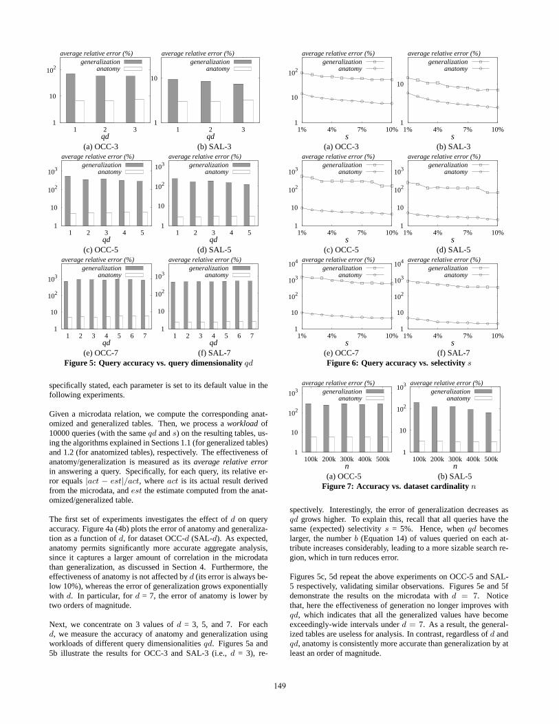
(e) OCC-7 (f) SAL-7Figure 5: Query accuracy vs. query dimensionalityqd

specifically stated, each parameter is set to its default value in thefollowing experiments.

Given a microdata relation, we compute the corresponding anat-omized and generalized tables. Then, we process aworkload of10000 queries (with the sameqd ands) on the resulting tables, us-ing the algorithms explained in Sections 1.1 (for generalized tables)and 1.2 (for anatomized tables), respectively. The effectiveness ofanatomy/generalization is measured as itsaverage relative errorin answering a query. Specifically, for each query, its relative er-ror equals|act − est|/act, whereact is its actual result derivedfrom the microdata, andest the estimate computed from the anat-omized/generalized table.

The first set of experiments investigates the effect ofd on queryaccuracy. Figure 4a (4b) plots the error of anatomy and generaliza-tion as a function ofd, for dataset OCC-d (SAL-d). As expected,anatomy permits significantly more accurate aggregate analysis,since it captures a larger amount of correlation in the microdatathan generalization, as discussed in Section 4. Furthermore, theeffectiveness of anatomy is not affected byd (its error is always be-low 10%), whereas the error of generalization grows exponentiallywith d. In particular, ford = 7, the error of anatomy is lower bytwo orders of magnitude.

Next, we concentrate on 3 values ofd = 3, 5, and 7. For eachd, we measure the accuracy of anatomy and generalization usingworkloads of different query dimensionalitiesqd. Figures 5a and5b illustrate the results for OCC-3 and SAL-3 (i.e.,d = 3), re-

102

10

110%7%4%1%

s


anatomy

10

110%7%4%1%

s


anatomy

(a) OCC-3 (b) SAL-3

103

102

10

110%7%4%1%

s


anatomy 103

102

10

110%7%4%1%

s


anatomy

(c) OCC-5 (d) SAL-5

104

103

102

10

110%7%4%1%

s


anatomy

104

103

102

10

110%7%4%1%

s


anatomy

(e) OCC-7 (f) SAL-7Figure 6: Query accuracy vs. selectivitys

103

102

10

1500k400k300k200k100k

n


anatomy

103

102

10

1500k400k300k200k100k

n


anatomy

(a) OCC-5 (b) SAL-5Figure 7: Accuracy vs. dataset cardinalityn

spectively. Interestingly, the error of generalization decreases asqd grows higher. To explain this, recall that all queries have thesame (expected) selectivitys = 5%. Hence, whenqd becomeslarger, the numberb (Equation 14) of values queried on each at-tribute increases considerably, leading to a more sizable search re-gion, which in turn reduces error.

Figures 5c, 5d repeat the above experiments on OCC-5 and SAL-5 respectively, validating similar observations. Figures5e and 5fdemonstrate the results on the microdata withd = 7. Noticethat, here the effectiveness of generation no longer improves withqd, which indicates that all the generalized values have becomeexceedingly-wide intervals underd = 7. As a result, the general-ized tables are useless for analysis. In contrast, regardless ofd andqd, anatomy is consistently more accurate than generalization by atleast an order of magnitude.

149

140k120k100k80k60k40k20k

0 3 4 5 6 7

d

I/O costgeneralization

anatomy

80k

60k

40k

20k

0 3 4 5 6 7

d


anatomy

(a) OCC-d (b) SAL-dFigure 8: I/O cost vs. the numberd of QI-attributes

180k

150k

120k

90k

60k

30k

0500k400k300k200k100k

n


anatomy

120k

100k

80k

60k

40k

20k

0500k400k300k200k100k

n


anatomy

(a) OCC-5 (b) SAL-5Figure 9: I/O cost vs. dataset cardinalityn

To study the impact of query selectivitys, we again examine themicrodata withd = 3, 5, and 7. Figures 6a-6f present the error ofboth techniques as a function ofs, for the 6 microdata tables used inFigure 5, respectively. The precision of both anatomy and general-ization improves ass increases, with anatomy being the clear win-ner. Finally, Figure 7 examines how the accuracy of each methodscales with the dataset cardinality. Again, Anatomy achieves sig-nificantly lower error in all cases.

In summary, we showed that anatomy allows very accurate ag-gregate analysis. Its error is usually smaller than that of general-ization by an order of magnitude. Furthermore, the effectivenessof anatomy is not affected by the dimensionalities of datasets andqueries.

6.2 Computation OverheadIn the sequel, we compare anatomy against generalization ontheI/O cost of computing publishable tables, with the page sizeset to4096 bytes, and a memory capacity of 50 pages. Figure 8 presentsthe comparison results asd varies from 3 to 7. Evidently, anatomyincurs significantly fewer I/Os. Figure 9 plots the I/O overhead asa function ofn. As predicted by Theorem 3, the cost of anatomyscales linearly withn, as opposed to the super-linear behavior ofgeneralization. For larged or n, anatomy is 10 times faster thangeneralization.

7. CONCLUSIONSAlthough generalization is a common methodology for protect-ing privacy, it loses considerable information in the microdata,and thus, prohibits effective data analysis. This paper developedanatomy, an innovative technique which preserves both privacy andcorrelation in the microdata, and hence, overcomes the drawbacksof generalization. Extensive experiments confirm that anatomy per-mits researchers to derive, from the published tables, highly accu-rate aggregate information about the unknown microdata, with anaverage error below 10% (as opposed to over 100% error of gener-alization).

As another important fact, anatomized tables can be computed inI/O cost linear to the database cardinality. In particular,these ta-bles have nearly optimal quality guarantees in correlationpreserv-ing. Furthermore, despite its rigorous theoretical justification, ouranatomizing algorithm is simple, and can be easily implemented inan existing database system.

This work also initiates several directions for future investigation.For example, in this paper, we focused on the case where thereisa single sensitive attribute. Extending our technique to multiplesensitive attributes is an interesting topic. As another direction, itwould be highly useful to study how anatomized tables can be uti-lized for effective mining of interesting patterns in the microdata,perhaps through minimization of other metrics of measuringinfor-mation loss (e.g., KL-divergence [7] and discernibility [4, 9]).

AcknowledgementsThis work was done when the authors were with the City Universityof Hong Kong, and supported by Grant CityU 1163/04E from theResearch Grant Council of the HKSAR government. We would liketo thank the anonymous reviewers for their insightful comments.

REFERENCES[1] C. C. Aggarwal. On k-anonymity and the curse of dimensionality. In

VLDB, pages 901–909, 2005.

[2] G. Aggarwal, T. Feder, K. Kenthapadi, R. Motwani, R. Panigrahy,D. Thomas, and A. Zhu. Anonymizing tables. InICDT, pages246–258, 2005.

[3] G. Arfken and H. Weber.Mathematical Methods for Physicists.Academic Press, 1995.

[4] R. Bayardo and R. Agrawal. Data privacy through optimalk-anonymization. InICDE, pages 217–228, 2005.

[5] B. C. M. Fung, K. Wang, and P. S. Yu. Top-down specialization forinformation and privacy preservation. InICDE, pages 205–216,2005.

[6] V. Iyengar. Transforming data to satisfy privacy constraints. InSIGKDD, pages 279–288, 2002.

[7] D. Kifer and J. E. Gehrke. Injecting utility into anonymized datasets.To appear in SIGMOD 2006.

[8] K. LeFevre, D. J. DeWitt, and R. Ramakrishnan. Incognito: Efficientfull-domaink-anonymity. InSIGMOD, pages 49–60, 2005.

[9] K. LeFevre, D. J. DeWitt, and R. Ramakrishnan. Mondrianmultidimensionalk-anonymity. InICDE, 2006.

[10] A. Machanavajjhala, J. Gehrke, and D. Kifer.l-diversity: Privacybeyondk-anonymity. InICDE, 2006.

[11] A. Meyerson and R. Williams. On the complexity of optimalk-anonymity. InPODS, pages 223–228, 2004.

[12] P. Samarati. Protecting respondents’ identities in microdata release.TKDE, 13(6):1010–1027, 2001.

[13] P. Samarati and L. Sweeney. Generalizing data to provide anonymitywhen disclosing information. InPODS, page 188, 1998.

[14] L. Sweeney. k-anonymity: a model for protecting privacy.International Journal on Uncertainty, Fuzziness, andKnowlege-Based Systems, 10(5):557–570, 2002.

[15] N. Thaper, S. Guha, P. Indyk, and N. Koudas. Dynamicmultidimensional histograms. InSIGMOD, pages 428–439, 2002.

[16] K. Wang, P. S. Yu, and S. Chakraborty. Bottom-up generalization: Adata mining solution to privacy protection. InICDM, pages 249–256,2004.

[17] X. Xiao and Y. Tao. Personalized privacy preservation.To appear inSIGMOD, 2006.

[18] C. Yao, X. S. Wang, and S. Jajodia. Checking fork-anonymityviolation by views. InVLDB.

150

Documents

Anatomy: Simple and Effective Privacy Preservation - Department of