Trace Gas Images of Alaska: CARVE and GMD Greenhouse gas  observations

John Miller, Colm Sweeney, Anna Karion, Tim Newberger, Sonja 

Wolter, Lori BruhwilerCIRES and NOAA/GMD

Chip Miller, Steve DinardoJPL

and the CARVE Science Team

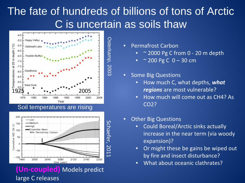
The fate of hundreds of billions of tons of Arctic C is uncertain as soils thaw

Osterkam

p, 2003

Soil temperatures are rising

1975 2005

Schaefer, 2011

(Un‐coupled) Models predict large C releases

• Permafrost Carbon• ~ 2000 Pg C from 0 ‐

20 m depth• ~ 200 Pg C  0 – 30 cm

• Some Big Questions• How much C, what depths, what 

regions

are most vulnerable?• How much will come out as CH4? As 

CO2?

• Other Big Questions• Could Boreal/Arctic sinks actually 

increase in the near term (via woody 

expansion)?

• Or might these be gains be wiped out 

by fire and insect disturbance?

• What about oceanic clathrates?

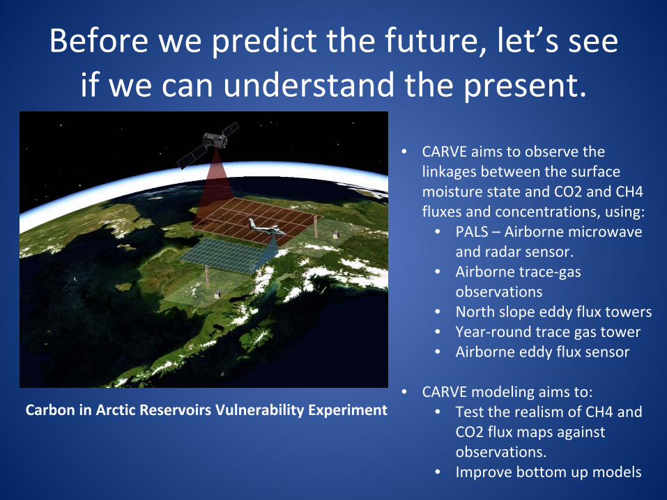
Before we predict the future, let’s see  if we can understand the present.

• CARVE aims to observe the 

linkages between the surface 

moisture state and CO2 and CH4 

fluxes and concentrations, using:

• PALS – Airborne microwave 

and radar sensor.

• Airborne trace‐gas 

observations

• North slope eddy flux towers• Year‐round trace gas tower• Airborne eddy flux sensor

• CARVE modeling aims to:• Test the realism of CH4 and 

CO2 flux maps against 

observations.

• Improve bottom up models

Carbon in Arctic Reservoirs Vulnerability Experiment

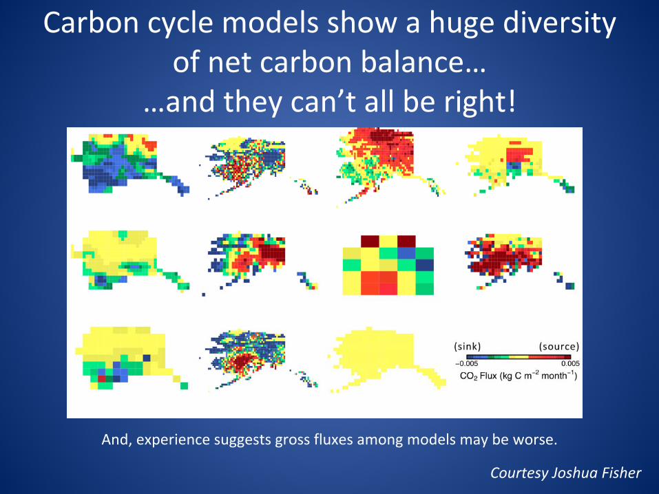
Carbon cycle models show a huge diversity  of net carbon balance…

…and they can’t all be right!

Courtesy Joshua Fisher

And, experience suggests gross fluxes among models may be worse.

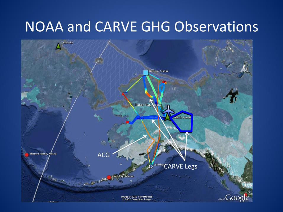
NOAA and CARVE GHG Observations

ACG

CARVE Legs

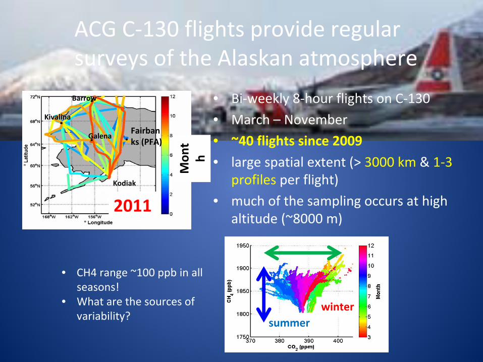
• Bi‐weekly 8‐hour flights on C‐130• March – November• ~40 flights since 2009• large spatial extent (> 3000 km & 1‐3 

profiles per flight)• much of the sampling occurs at high 

altitude (~8000 m)2011

Fairban

ks (PFA)

Kivalina

Barrow

Kodiak

Galena

Mon

th

ACG C‐130 flights provide regular  surveys of the Alaskan atmosphere 

summerwinter

• CH4 range ~100 ppb in all 

seasons!

• What are the sources of 

variability?

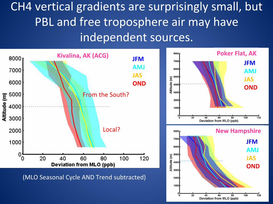
CH4 vertical gradients are surprisingly small, but  PBL and free troposphere air may have 

independent sources.

(MLO Seasonal Cycle AND Trend subtracted)

Poker Flat, AKKivalina, AK (ACG)

New Hampshire

JFMAMJJASOND

JFMAMJJASOND

JFMAMJJASOND

From the South?

Local?

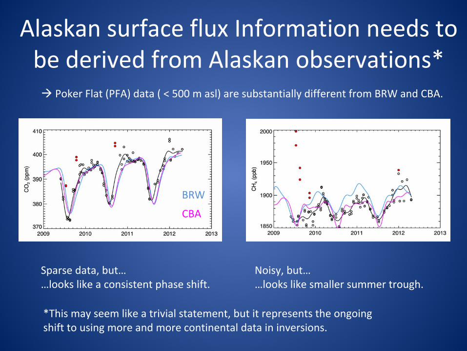
Alaskan surface flux Information needs to  be derived from Alaskan observations*

Poker Flat (PFA) data ( < 500 m asl) are substantially different

from BRW and CBA.

BRW

CBA

Sparse data, but……looks like a consistent phase shift.

Noisy, but……looks like smaller summer trough.

*This may seem like a trivial statement, but it represents the ongoing 

shift to using more and more continental data in inversions.

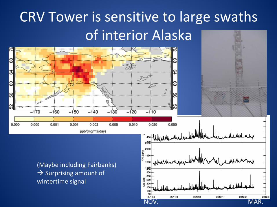
CRV Tower is sensitive to large swaths  of interior Alaska

(Maybe including Fairbanks) Surprising amount of 

wintertime signal

NOV. MAR.

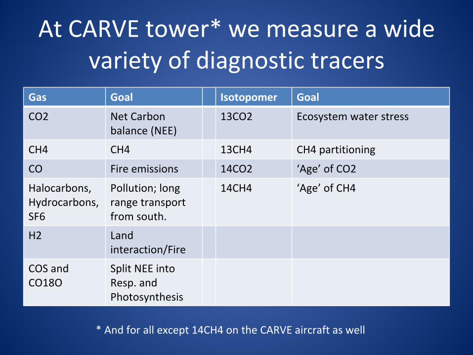
At CARVE tower* we measure a wide  variety of diagnostic tracers

Gas Goal Isotopomer Goal

CO2 Net Carbon 

balance (NEE)

13CO2 Ecosystem water stress

CH4 CH4 13CH4 CH4 partitioning

CO Fire emissions 14CO2 ‘Age’

of CO2

Halocarbons, 

Hydrocarbons, 

SF6

Pollution; long 

range transport 

from south.

14CH4 ‘Age’

of CH4

H2 Land 

interaction/Fire

COS and 

CO18O

Split NEE into 

Resp. and 

Photosynthesis

* And for all except 14CH4 on the CARVE aircraft as well

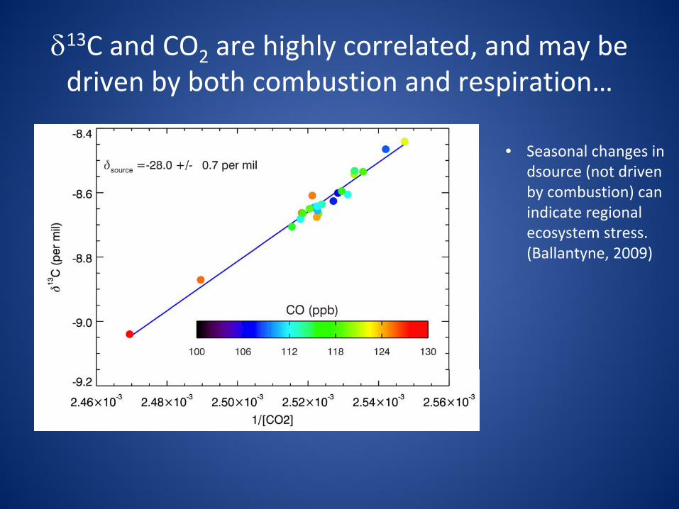
13C and CO2

are highly correlated, and may be  driven by both combustion and respiration…

• Seasonal changes in 

dsource

(not driven 

by combustion) can 

indicate regional 

ecosystem stress. 

(Ballantyne, 2009)

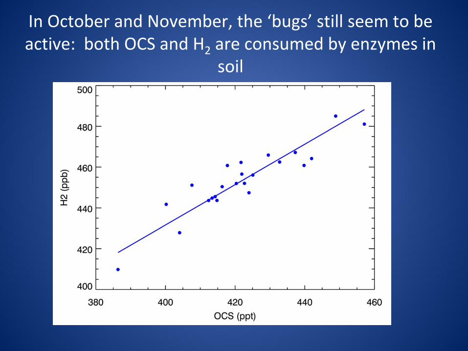
In October and November, the ‘bugs’

still seem to be  active:  both OCS and H2

are consumed by enzymes in  soil

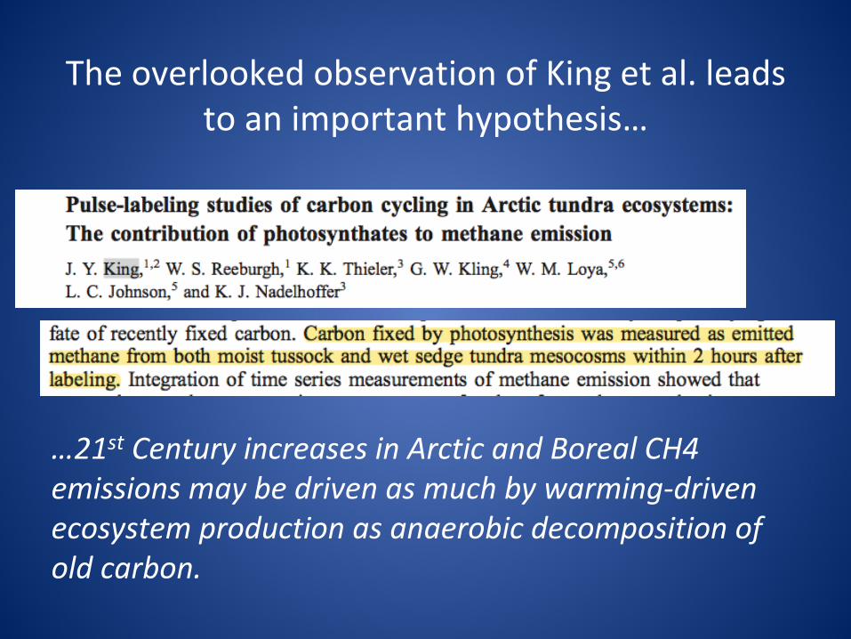
The overlooked observation of King et al. leads  to an important hypothesis…

…21st

Century increases in Arctic and Boreal CH4  emissions may be driven as much by warming‐driven 

ecosystem production as anaerobic decomposition of  old carbon.

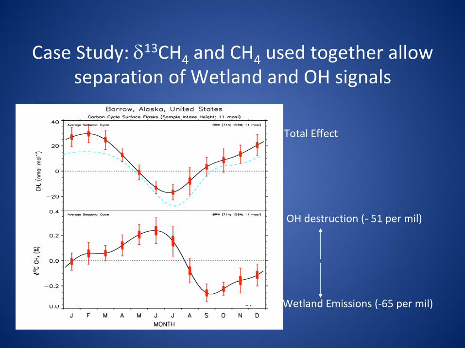
Total Effect

OH destruction (‐

51 per mil)

Wetland Emissions (‐65 per mil)

Case Study: 13CH4

and CH4

used together allow  separation of Wetland and OH signals

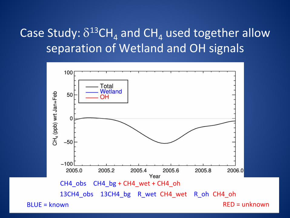
Case Study: 13CH4

and CH4

used together allow  separation of Wetland and OH signals

CH4_obs

= CH4_bg

+ CH4_wet + CH4_oh13CH4_obs

= 13CH4_bg

+ R_wet*CH4_wet

+ R_oh*CH4_ohBLUE = known RED = unknown

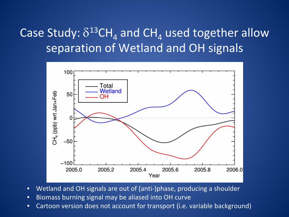
Case Study: 13CH4

and CH4

used together allow  separation of Wetland and OH signals

• Wetland and OH signals are out of (anti‐)phase, producing a shoulder• Biomass burning signal may be aliased into OH curve• Cartoon version does not account for transport (i.e. variable background)

We want to use 14CH4

to answer: Is the wetland signal is modern?

~50 ppb

A.

If the 14CH4 is aseasonal, this suggests that Wetland CH4 is modernB.

If 14CH4 dips in fall, this suggests a substantial fraction of old CH4.C.

Quantifying the old CH4 fraction, depends on the 14C of the organic matter. 

14CH4Modern

Old

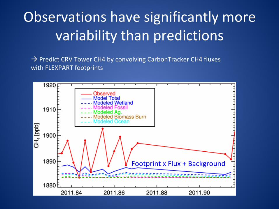
Observations have significantly more  variability than predictions

Footprint x Flux + Background

Predict CRV Tower CH4 by convolving CarbonTracker CH4 fluxes 

with FLEXPART footprints

Summary

• CARVE and new GMD measurement programs  will allow much better sensing of Alaskan 

carbon balance.• We are still confronted with the Goldilocks 

issue:  (not too close to sources, not too far.   Just right.)

Outline• Motivation

– Understanding arctic and boreal carbon cycling:  Baselines  and sensitivities

• Existing and planned GHG observations– Surface sites

• CARVE tower (CRV)• Barrow (BRW), Cold Bay (CBA)

– Airborne observations• Poker Flat (PFA)• Alaska Coast Guard  C‐130‐of‐opportunity (ACG)• (2011 CARVE Aircraft)

• Preliminary data analysis– Multi‐species (including isotopic) analysis– Lagrangian and Eulerian

modeling

Notes• What are the big questions for Boreal and Arctic Carbon?

– Changes in C‐cycling with warming:• Permafrost release as  CO2 or CH4 as active layer increases with

depth and time• Increased growing season:  more NPP: released as CO2 or CH4.• Do oceanic clathrates

(ch4 . X H2o) play a role?• What is the role of fire in carbon balance?• Can current models represent the current state; ~decadal trends;

seasonal and interannual

variability?– C‐cycle is a first order uncertainty in climate prediction!!

• How can existing and planned NOAA+CARVE atmospheric gas obs help

to answer these questions?– Survey of ongoing NOAA/GMD measurements in Alaska/Motivation

• GE map with permafrost layer; NOAA site layer (PFA, CRV tower etc.); and ACG flights; and CARVE flights• (also CARVE remote sensing obs?)

– Generally: constrain emission estimates:• Test emission models of CO2, CH4 and CO by fwd transport compared to observations• Direct calculation of emission by inverse modeling• Role of ancillary gases/isotopes for process attribution:

– 14CH4 and 14CO2:  age of released carbon – new NPP or recently emerged buried C.– 13CO2:  seasonal and interannual

water stress– 13CH4:  CH4 consumption by OH, biomass burning and wetland production– CH3D: wetland processes??– COS + CO18O:  Photosynthesis v. respiration in net carbon exchange.– Anthro

tracers:  long range and local pollution transport –

screening and/or deconvolution• Correlation of CO2, CH4 fluxes (inverse) or just concentrations with remotely sensed surface observations of temp and 

moisture – fractional innundation

maps from Ronny and Kyle??

‐‐add wind fields ‐‐

also do GFED fires??

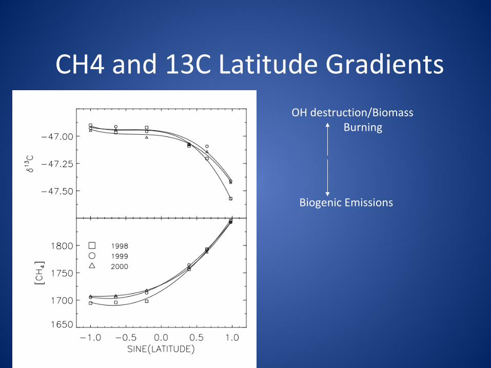
CH4 and 13C Latitude GradientsOH destruction/Biomass

Burning

Biogenic Emissions

NPSP

Warming temperatures are also likely  to:

Sequester carbon by: extending the growing season

expanding the boreal (tree) zone

and release carbon by: increased fire frequency

increased insect outbreaks also physical climate changes:

changes in albedo (higher –

snowshedding evergreen trees)

sensible heat flux (higher due to boreal forest  high WUE/low conductance.)

atmos. Circulation 

changes