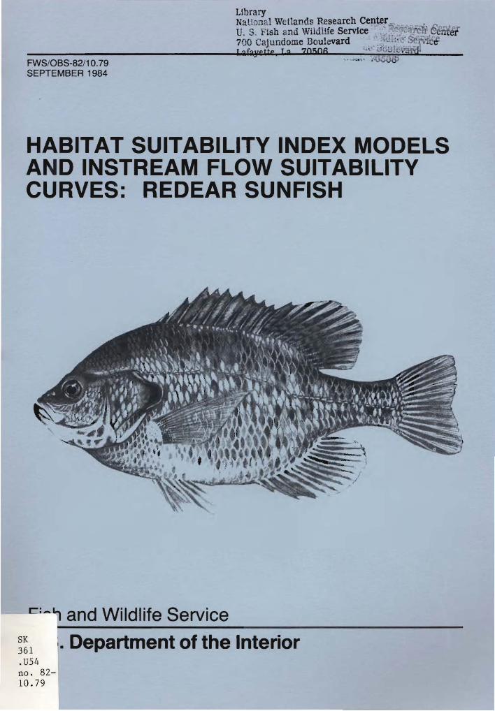
HABITAT SUITABILITY INDEX MODELSAND INSTREAM FLOW SUITABILITYCURVES: REDEAR SUNFISH

', . .. :.~

LibraryNational W tlands Research Center;U, .. . Fish nd wuaure service . ,' l~'•.~-.,~~:~~

700 Cajundome Boulevard , ; "'~ .""::\ t.I'Myette I a 70506 .~ ". ,:, .- .. .)::a~

FWS/OBS-82/1 0.79SEPTEMBER 1984

1:::_, and Wildlife Service

~~1 I . Department of the Interior. U54no. 82­10.79

MODEL EVALUATION FORM

Habitat models are designed for a wide variety of planning applica­tions where habitat information is an important consideration in thedecision process. However, it is impossible to develop a model thatperforms equally well in all situations. Assistance from users andresearchers is an important part of the model improvement process. Eachmodel is published individually to facilitate updating and reprinting asnew information becomes available. User feedback on model performancewill assist in improving habitat models for future applications. Pleasecomplete this form following application or review of the model. Feelfree to include additional information that may be of use to either amodel developer or model user. We also would appreciate information onmodel testing, modification, and application, as well as copies of modifiedmodels or test results. Please return this form to:

Habitat Evaluation Procedures GroupU.S. Fish and Wildlife Service2627 Redwing Road, Creekside OneFort Collins, CO 80526-2899

Thank you for your assistance.

Species ___

Habitat or Cover Type(s)

GeographicLocation --------------------

Type of Application: Impact Analysis Management Action AnalysisBaseline Other --------------------------------------------------Variables Measured or Evaluated ------------------------------------

Was the species information useful and accurate? Yes No

If not, what corrections or improvements are needed?-------------------

Were the variables and curves clearly defined and useful? Yes No

If not, how were or could they be improved? ___

Were the techniques suggested for collection of field data:Appropriate? Yes NoClearly defined? Yes NoEasily applied? Yes No

If not, what other data collection techniques are needed?

Were the model equations logical? Yes NoAppropriate? Yes No

How were or could they be improved?

Other suggestions for modification or improvement (attach curves,equations, graphs, or other appropriate information)

Additional references or information that should be included in the model:

Model Evaluater or Reviewer Date------------------------ -------------

Agency _

Address

Telephone Number Comm:-----------------FTS _

FWS/OBS-82/10.79September 1984

HABITAT SUITABILITY INDEX MODELS AND INSTREAM FLOWSUITABILITY CURVES: REDEAR SUNFISH

by

Kathleen A. TwomeyWyoming Cooperative Fishery Unit

University of WyomingLaramie, WY 82071

Glen GebhartO. Eugene Maughan

Oklahoma Cooperative Fishery Research UnitOklahoma State University

Stillwater, OK 74074

and

Patrick C. NelsonInstream Flow and Aquatic Systems Group

Western Energy and Land Use TeamU.S. Fish and Wildlife ServiceDrake Creekside Building One

2627 Redwing RoadFort Collins, CO 80526-2899

Western Energy and Land Use TeamDivision of Biological Services

Research and DevelopmentFish and Wildlife Service

U.S. Department of the InteriorWashington, DC 20240

This report should be cited as:

Twomey, K. A., G. Gebhart, O. E. Maughan, and P. C. Nelson. 1984. Habitatsuitability index models and instream flow suitability curves: Redearsunfish. U.S. Fish Wildl. Servo FWS/OBS-82/10.79. 29 pp.

1981. Standards for the development of103 ESM. U.S. Fish Wild1. Serv., Div.

PREFACE

The Habitat Suitability Index (HSI) models presented in this publicationaid in identifying important habitat variables. Facts, ideas, and conceptsobtained from the research literature and expert reviews are synthesized andpresented in a format that can be used for impact assessment. The models arehypotheses of species-habitat relationships, and model users should recognizethat the degree of veracity of the HSI model, SI graphs, and assumptions willvary according to geographical area and the extent of the data base for indi­vidual variables. After clear study objectives have been set, the HSI modelbuilding techniques presented in U.S. Fish and Wildlife Service (1981)1 andthe general guidelines for modifying HSI models and estimating model variablespresented in Terrell et al. (1982)2 may be useful for simplifying and applyingthe model s to specific impact assessment problems. Simpl ified model s shouldbe tested with independent data sets, if possible. Statistically-derivedmodels that are an alternative to using Suitability Indices to calculate anHSI are referenced in the text.

A brief discussion of the appropriateness of using selected SuitabilityIndex (SI) curves from HSI models as a component of the Instream Flow Incre­mental Methodology (IFIM) is provided. Additional SI curves, developed specif­ically for analysis of redear sunfish habitat with IFIM, also are presented.

Model reliability is likely to vary in different geographical areas andsituations. The U.S. Fish and Wildlife Service encourages model users toprovide comments, suggestions, and test results that may help us increase theutility and effectiveness of this habitat-based approach to impact assessment.Please send comments to:

Habitat Evaluations Procedures Group orInstream Flow and Aquatic Systems Group

Western Energy and Land Use TeamU.S. Fish and Wildlife Service2627 Redwing RoadFort Collins, CO 80526-2899

1U.S. Fish and Wildlife Service.habitat suitabi 1ity index mode 1s.Ecol. Servo n.p.

2Terrell, J. W., T. E. McMahon, P. D. In ski p, R. F. Raleigh, and K. L.Williamson. 1982. Habitat suitability index models: Appendix A. Guidelinesfor riverine and lacustrine applications of fish HSI models with the HabitatEvaluation Procedures. U.S. Fish Wildl. Servo FWS/OBS-82/10.A. 54 pp.

iii

iv

CONTENTS

PREFACE iiiACKNOWLEDGMENTS vi

HABITAT USE INFORMATION 1Genera1 1Age, Growth, and Food 1Reproduct ion 2Specifi c Habi tat Requi rements 2

HABITAT SUITABILITY INDEX (HSI) MODELS. 5Model Applicability............................................... 5Model Description................................................. 5Model Description - Riverine...................................... 6Model Description - Lacustrine. 6Suitability Indices of Selected Variables 9River.ine Model 14Lacustri ne Model.................................................. 19Interpret i ng Model Outputs 19

ADDITIONAL HABITAT MODELS.... 20Modell ,. . . .. .. . .. .. . . . .. . .. . . . . .. 20Model 2 20Model 3 21

INSTREAM FLOW INCREMENTAL METHODOLOGY (IFIM) 21Suitability Index Graphs as Used in IFIM . 22Avail abi·l i ty of Graphs for Use in I FIM 24

REFERENCES 26

v

ACKNOWLEDGMENTS

We would like to thank R. O. Anderson, Missouri Cooperative FisheryResearch Unit; J. P. Clugston, National Fishery Research Laboratory,Gainesville; and R. L. Wilbur, Alaska Department of Fish and Game for theirhelpful comments and suggestions. We are indebted to R. Stuber, U.S. ForestService, for development of an earlier draft and literature review and initialwork on suitability graphs. C. Short and T. Rosenthal provided editorialassistance. Word processing was by C. J. Gulzow and D. E. Ibarra. The coverillustration was done by Duane Raver, U.S. Fish and Wildlife Service.

vi

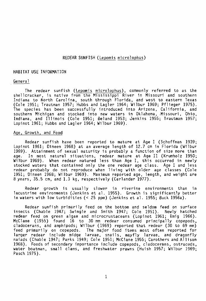
REDEAR SUNFISH (Lepomis microlophus)

HABITAT USE INFORMATION

General

The redear sunfish (Lepomis microlophus), commonly referred to as theshellcracker, is native from the Mississippi River in Missouri and southernIndiana to North Carolina, south through Florida, and west to eastern Texas(Cole 1951; Trautman 1957; Hubbs and Lagler 1964; Wilbur 1969; Pflieger 1975).The species has been successfully introduced into Arizona, California, andsouthern Michigan and stocked into new waters in Oklahoma,Missouri, Ohio,Indiana, and Illinois (Cole 1951; Beland 1953; Jenkins 1955; Trautman 1957;Lopinot 1961; Hubbs and Lagler 1964; Wilbur 1969).

Age, Growth, and Food

Redear sunfish have been reported to mature at Age I (Schoffman 1939;Lopinot 1961; Dineen 1968) at an average length of 12.7 cm in Florida (Wilbur1969). Attainment of sexual maturity is probably a function of size more thanage. In most natural situations, redear mature at Age II (Krumholz 1950;Wnbur 1969). When redear matured less than Age I, this occurred in newlystocked waters that contained only the one redear age class. Age I and lessredear probably do not reproduce when living with older age classes (Cole1951; Dineen 1968; Wilbur 1969). Maximum reported age, length, and weight are8 years, 35.5 cm, and 1.3 kg, respectively (Carlander 1977).

Redear growth is usually slower in riverine environments than inlacustrine environments (Jenkins et al. 1955). Growth is significantly betterin waters with low turbidities « 25 ppm) (Jenkins et al. 1955; Buck 1956a).

Redear sunfi sh primari ly feed on the bottom and seldom feed on surfaceinsects (Chable 1947; Swingle and Smith 1947; Cole 1951). Newly hatchedredear feed on green algae and microcrustaceans (Lopinot 1961; Emig 1966).McClane (1955) found 16 to 30 mm redear consumed principally copepods,cladocerans, and amphipods; Wilbur (1969) reported that redear (30 to 69 mm)feed primari lyon copepods. The major food items most often reported forlarger redear include midge larvae, snails, mayfly larvae, and dragonflynaiads (Chable 1947; Parks 1949; Cole 1951; McClane 1955; Carothers and Allison1968). Foods of secondary importance include copepods, cladocerans, ostracods,water boatman, small clams, and freshwater prawns (Huish 1957; Wilbur 1969;Pasch 1975).

1

Reproduction

Redear sunfish display great variation in spawning season. Within mostof their range, redear sunfish usually begin to spawn in May to June, and maycontinue to spawn until September (Schoffman 1939; Dineen 1968; Pflieger1975). Redear may spawn sparingly during the summer and heavily in the earlyfall (Swingle 1949). In Florida redear sunfish begin to spawn in late Februaryor early March and continue to spawn intermittently until October 1 (Clugston1966). In the northern reaches of their distribution (Michigan, Illinois, andIndiana), nesting begins in May to July and generally does not extend intolate summer (Krumholz 1950; Cole 1951; Childers 1967).

The eggs are laid in saucer-shaped nests, fanned free of debris (Gresham1965; Wilbur 1969). Redear tend to be community spawners, often with nestsonly a few inches from each other (McCl ane 1955; Clugston 1966; Emi g 1966;Pflieger 1975). Nests have been found at water depths from approximately 5 to10 cm (Swingle and Smith 1947; Gresham 1965; Emig 1966) to 4 to 6 m (Wilbur1969). Gresham (1965) and Clugston (1966) reported that nests were usually atwater depths of 45 to 90 cm. McClane (1955) reported that spawning most oftenoccurred at depths of 91 to 122 cm in the St. Johns River; Swingle and Smith(1947) reported that nests in ponds were most often at water depths of at1east 183 cm.

Redear use a wide range of spawning habitats and nesting substrates.Nests have been reported on substrates of sand, sandy-c 1ay, mud, 1i mestone,shells, and gravel with no vegetation (McClane 1955; Emig 1966; Wilbur 1969),often in locations exposed to the sun (Childers 1967). Nests are often withinor along the edge of water lilies, Pancium, Chara, Vallesneria, and fallentrees and old pilings in Florida (McClane 1955; Wilbur 1969).

After the eggs are fertilized, the male remains above the nest guardingand fanning the eggs until they hatch, which takes 6 to 10 days, depending onthe water temperature. An alpha-threshold temperature necessary for 50%hatching is reported as 18.3° C (Childers 1967). The highest percent ofnormal fry resulted at an incubation temperature of 23.6° C in an experimentaltemperature range of 22.3 to 28.6° C (Childers 1967). It is assumed thatoptimum temperatures for successful incubation and subsequent hatching are 21to 24° C, based on field observations by Swingle (1949), Cole (1951), Lopinot(1961, 1972), Clugston (1966), and Wilbur (1969), although Clugston (1966)reported that spawning occurred at temperatures as high as 32.2° C. Afterhatching, the fry remain on the nest for about a week (Lopinot 1961). Thereappears to be little difference, if any, in the spawning requirements ofredear in lacustrine and riverine environments.

Specific Habitat Requirements

Redear sunfish prefer warm, large lakes, bayous, marshes, and reservoirswith vegetated shallow areas and clear water (Chable 1947; Cole 1951; Finnellet al. 1956; Lopinot 1961). In riverine habitats, redear sunfish preferlarge, clear, low gradient streams and rivers with sluggish currents and someaquatic vegetation. Redear sunfish prefer habitats with no noticeable currents(McClane 1955; Trautman 1957; Pflieger 1975). Bailey et al. (1954) reported

2

that redear occurred in areas with no to moderate current velocities (0 toapproximately 10 cm/sec). In streams, redear are more likely to be inprotected bays and overflow pool s than in the main stream channel (Chable1947; McClane 1955; Pflieger 1975; Smith 1979).

Redear sunfish appear to prefer riverine pools with aquatic vegetation(Smith 1979) and do best in lacustrine waters with at least some vegetation(Trautman 1957; Pflieger 1975). The redear is also known to congregate aroundbrush, stumps, and logs (Trautman 1957; Lopinot 1961). Redear adults typicallyoccur in deeper, open waters and only move shoreward to spawn (Chable 1947;Cole 1951; McClane 1955; Lopinot 1961; Wilbur 1969), although Wilbur (1969)reported that greater densities of redear occurred in the peripheral deepwater areas near submergent vegetation. Wilbur (1969) concluded that, exceptduring spawning season, emergent vegetation was of lesser importance to redearthan open water areas. Vegetation enhances redear habitat by providing coverand substrate for food (Chable 1947). Centrarchids appear to reach theirgreatest abundance in lakes where large numbers of invertebrates are associatedwith vegetation (Chable 1947; Wilbur 1969; Colle and Shireman 1980).

The condition of redear is influenced by the amount of vegetation inFlorida (Colle and Shireman 1980). Redear sunfish are influenced to a greaterextent by the amount of vegetation in the water column than by the percentbottom cover. Colle and Shireman (1980) indicated that habitats with moderatelevels of Hydrilla result in improved condition and growth for redear sunfish> 100 mm. However, if plants occupy the entire water column, a marked reduc­tion in both growth and condition of redear occurs. Redear sunfish were ofaverage or above average condi t i on when Hydri 11 a covered up to 78% of thebottom and surface matting was present in 23% of the lake. Lower conditionfactors were evident when 95% of the lake bottom was covered and 80% of thesurface was matted. When the water column is full of Hydrilla, the Hydrillaprobably becomes a physical constraint on foraging efficiency by eliminatingthe foraging gradient between open water and submersed macrophytes.

Redear sunfi sh grew faster and reproduced more abundantly in averageturbidities of s 25 ppm (Buck 1956b). Although redear sunfish were reportedto reproduce and young redear were recovered in a pond with a high turbidity(174 ppm) in one study, the critical level for successful reproduction andgrowth over time is probably between 75 and 100 ppm (Buck 1956b). Althoughredear prefer clear waters, redear sunfish seem to be more tolerant ofturbidity than bass or bluegills (Buck 1956b; Smith 1979).

Redear sunfish are usually outnumbered by other centrarchid species whenthey occur in the same freshwaters; but in marshes and brackish waters, redeargenera lly have 1arger standi ng crops than the other centrarchi ds present(Horel 1967; Dineen 1968; Wilbur 1969). Redear are probably the mostsalinity-tolerant species of all the centrarchids and survive without apparentdiscomfort in brackish water (Bailey et al. 1954; Wilbur 1969). Redear arefound living in the tidewater of the Escambia River, Florida, where salinitiesranged up to 24.4 ppt (Bailey et al. 1954). Bailey et al. (1954) classifiedredear sunfi sh as facultative invaders of brackish water. They frequentlyinvade, probably for a considerable time, into water of low salinity (i.e., atleast 4.5 ppt). Redear occur at salinities from 2.6 to 6.7 ppt in Louisiana

3

(Geagan 1962) and at salinities up to 12.3 ppt in Florida gulf coast marshes,although 90% of the redear collected in this survey were from water with asalinity of less than 5 ppt (Kilby 1955).

The highest standing crops of warmwater sport fishes (including sunfishes)occur in waters of moderate alkalinity of 100 to 350 ppm (Jenkins 1976). Thefollowing environmental variables have a positive effect on redear standingcrop: increased mean depth; increased storage ratio (lower water exchangerate); and longer growing season (Jenkins 1968,1970). Water level fluctua­tions and shore development have a negative effect on redear standing crop. Apositive association between length of growing season (number of frost-freedays) and sunfish standing crop was reported by Jenkins and Morais (1971). Nosunfishes were harvested in reservoirs with growing seasons of less than140 days. Annual harvest rates increase most rapidly when the growing seasonis 180 to 240 days long; therefore, it is assumed that optimal growing seasonfor redear is > 180 days.

There is little information on the dissolved oxygen (D.O.) requirementsof redear sunfish, but it is assumed that their D.O. needs are similar tothose of bl ueq i l l s . The first external sign of stress in bluegills occurswhen oxygen levels drop to 5 mg/l; at 3 mg/l D.O., bluegills begin to inter­mittently swim to the surface; and, at 1 mg/l D.O., feeding ceases (Petit1973). The critical level of dissolved oxygen for bluegills is 0.75 to1.50 mg/l at 25° C and 2.0 mg/l at 35° C (Moss and Scott 1961). A pH range ofapproximately 6.7 to 8.6, with an extreme range of 6.3 to 9.0 is thought tosafely support a good mixed fish fauna (McKee and Wolf 1963). Thus, it isassumed redear populations would be unaffected by these pH ranges.

Adult. The best growth for redear was reported to occur at temperaturesof 23.9° C by Rounsefell and Everhart (1953), but Leidy and Jenkins (1977)reported the optimum or preferred temperature for growth of bluegill s , sma11­mouth bass, and largemouth bass to be 27° C. At acclimation temperatures of16° C, 21° C, and 26° C the redear sunfish selected temperatures at 22° C,23° C, and 28° C, respectively (Hill et al. 1975). From this information theauthor assumes optimal temperatures for redear growth range from 24 to 27° C.Cole (1951) reported that bacterial fin rot and fungus attacked redear sunfishalmost continuously in aquaria once temperatures fall below 14.4° C. Below6.6° C, redear were inactive and did not feed. It is assumed that redeargrowth ceases when temperatures fall below 10° C, as is true for bluegill s(Anderson 1958). A lower lethal temperature of 6.5° C was determined inreservoirs by Leidy and Jenkins (1977). Redear sunfish are susceptible torapid temperature changes (Swingle 1949; Rounsefell and Everhart 1953).

Embryo. Embryonic development is inhibited by turbidity levels> 175 ppm,and optimum turbidity levels are < 25 ppm (Buck 1956a). It is assumed thatcurrent velocities of < 1 cm/sec for embryos are preferred because redearsunfish inhabiting streams move shoreward into coves and bays to spawn (McClane1955) and aeration of the eggs is provided by the guarding male. Redearsunfi sh nest from several centimeters to 6 min depth; therefore, reservoi rdrawdowns > 6 m would probably destroy all nests. 'To ensure optimum survival,reservoir drawdown should probably not occur during the spring and earlysummer.

4

Fry. Young redea r sunfi sh are most often found among the submergentvegetation in the littoral zone (McClane 1955; Wilbur 1969). Temperature,turbidity, and velocity criteria for redear fry are assumed to be similar tothose for the embryo life stage.

Juvenile. Juvenile habitat requirements are assumed to be similar tothose of adult redear sunfish.

HABITAT SUITABILITY INDEX (HSI) MODELS

Model Applicabilitx

Geographic area. This model is applicable throughout North Americanwaters within the native and introduced range of redear sunfish. The standardof comparison for each individual variable is the optimum value that occursanywhere within this geographic range.

Season. The model provides an index for a riverine and lacustrine habitatbased on the habitats ability to support all life stages of redear sunfishthroughout the year.

Cover types. The model is applicable in riverine and lacustrine, asdescribed by Cowardin et al. (1979).

Minimum habitat area. Minimum habitat area is defined as the nn mmumarea of contiguous suitable habitat that is required for a population tomaintain itself indefinitely. The minimum habitat area necessary for a redearsunfish population has not been established.

Verification level. The model represents an interpretation of howselected environmental factors limit potential carrying capacity for redearsunfi sh. The acceptance 1eve1 of the 1acustri ne and ri veri ne models is thatit produce an index between 0 and 1 that the authors believe have a positiverelationship to carrying capacity for redear sunfish. This model has not beensubjected to field testing or application.

Model Description

Riverine and lacustrine Habitat Suitability Index (HSI) models arepresented. These models condense the preceding observations into a set ofmeasurable habitat variables. The models are structured to produce an indexof redear sunfish habitat quality between 0.0 (unsuitable) and 1.0 (optimum).A positive relationship between HSI and carrying capacity is assumed but hasnot been demonstrated. Habitat variables believed to be important in limitingdistribution, abundance, or survival of redear sunfish are included in themodels. An assumed functional relationship between each habitat variable andhabitat suitability is represented in a variable suitability index (SI) graph.The model is likely to provide the most accurate description of carryingcapacity when all of the variables have extreme SI values; i.e., either nearoptimum or near unsuitable.

5

Redear sunfish habitat quality is represented by food, cover, waterqua1i ty, and reproduction components. Component ratings were deri ved fromindividual variable suitability indices (Figs. 1 and 2). Reasons for placingindividual variables in specific components and assumed variable interactionsare described below.

Model Descr.iption - Riverine

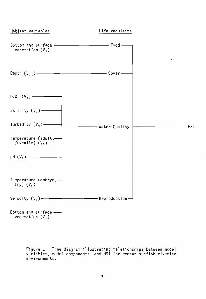
The structure of the riverine HSI model for redear sunfish is illustratedin Figure 1.

Food component. Bottom and surface vegetation (V 1 ) are part of the food

component because redear sunfish condition and growth are positively influencedby a moderate level of vegetation that supports a large number of inverte­brates. Too much vegetation can decrease foraging efficiency by redear andhave a negative influence on growth and condition.

Cover component. Percentage of habitat> 2 m (depth) (V ll ) is included

in the cover component because redear sunfish adults and juveniles usuallyoccur in the deeper waters of rivers and only come shoreward or utilize shallowlittoral areas for spawning.

Water quality component. Dissolved oxygen (V z ) , turbidity (V 4 ) , tempera­

ture for adults/juveniles (V s ) , and pH (V s ) are included in the water quality

component because they affect growth, survival, and/or distribution of redearsunfish. Salinity (V 1 ) is in the water quality component because redear

sunfish are probably the most salinity-tolerant centrarchid. They are oftenfound in brackish marshes and tidewaters, where they generally occur in greaterstanding crops than other centrarchids. This variable should only be consid­ered in areas where salinity is a factor.

Reproduction component. Temperature for spawning and incubation (V 6 ) is

included in the reproduction component because it influences spawning time,incubation length, and hatching success. Redear sunfish are also susceptibleto rapid temperature changes. Velocity (V 9 ) is considered part of the repro-

duction component because nests are built in waters with no to very slow watercurrents, and adult males guard the nest and aerate the eggs for a time.Therefore, flowing waters are not needed for aeration and high velocitieswould prevent nest construction or 1imit the time that the males attend thenest. Although it is not critical for nesting substrate, bottom and surfacevegetation (V 1 ) are part of this component because they provide cover for fry,

substrate for green algae and microcrustaceans on which fry feed, and nestsoften are located along the edges of vegetation or within its rhizomes.

Model Description - Lacustrine

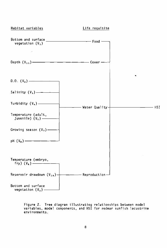
The structure of the 1acustri ne HSI model for redear sunfi sh is ill us­trated in Figure 2.

6

Habitat variables Life requisite

Bottom and surface ----------- Foodvegetation (VI)

Depth (V 11) -------------- Cove r ------i

D.O. (V2 ) - - - - ----l

Salinity (V3)---~

Turbidity (V,.) -----11---- Water Quality+---------- HSI

Temperature (adult,­juvenile) (V s )

pH (V 8) --------'

Temperature (embryo,fry) (V 6 )

Velocity (V 9 ) -------1f----------- Reproduction

Bottom and surfacevegeta t ion (V 1 )

Figure 1. Tree diagram illustrating relationships between modelvariables, model components, and HSI for redear sunfish riverineenvironments.

7

Habitat variables LHe regui site

Bottom and surface Foodvegetation (VI)

Depth (V ll ) - - - - - - - - - - - - - Cover

D.O. (V2 ) --------.

Salinity (V3)--------~

Turbidity (V~)--------~

/------ Wa te r Qua 1i ty -t----------- HS I

Temperature (adult,juvenil e) (V s ) ------I

Growing season (V7)-----~

pH (V8) --------'

Temperature (embryo,fry) (V,) ----------,

Reservoi r drawdown (V 10) -+------ Reproduct ion

Bottom and surfacevegetat ion (VI) ----'

Figure 2. Tree diagram illustrating relationships between modelvariables, model components, and HSI for redear sunfish lacustrineenvironments.

8

Food component. Only bottom and surface vegetation (Vi) are included in

this component. As in the riverine model, moderate vegetation positivelyi nfl uences redear growth and condition because it supports an invertebratepopulation important as a food source.

Cover component. Percentage of habitat> 2 m (depth) (Vii) is important

as cover because adul t and juveni 1e redear sunfi sh prefer deeper water andonly move shoreward for spawning.

Water quality component. Dissolved oxygen (V z ) , turbidity (V 4 ) , tempera­

ture for adults/juveniles (V s ) , and pH (Vs ) are included in the water quality

component because they influence growth, survival, and distribution of redearsunfish. Salinity (V 3 ) can be important to water quality in some areas;

however, redear sunfish are relatively salinity-tolerant and occur in brackishmarshes and lakes. Growing season (V 7 ) is included in this component because

redear growth and standing crop are positively correlated to length of growingseason (number of frost-free days).

Reproduction component. As in the riverine model, temperature for embryo/fry (V 6 ) is important in the reproduction component because it influences

spawning time, incubation length, and hatching success. Reservoir drawdown(V 1 D) can negatively affect reproductive success when spawning occurs in

shallow water and nests and eggs become exposed when water levels drop.Redear sunfish spawn in coves, bays, and shorel ines at depths < 6 m. Bottomand surface vegetat ion (V 1) offer protect i on for fry, a substrate for food,

and nests often are located near or within vegetation.

Suitability Indices of Selected Variables

Suitability indices for selected variables are given below. The "R" forriverine and "L" for lacustrine under the heading "hab i t.a t" describe the typeof habitat where the variable should be measured. Sources of data used todevelop the suitability indices are listed in Table 1.

9

Habitat Variable Suitability graph

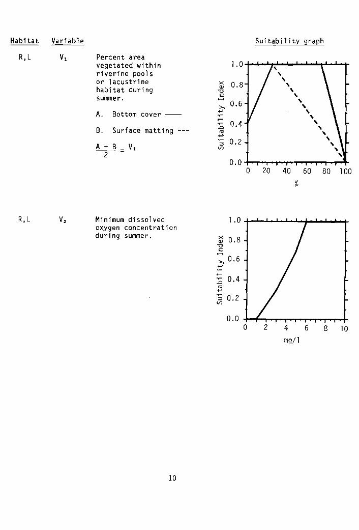
R,L Vl Percent areavegetated withinriverine poolsor lacustrinehabitat duringsummer.

A. Bottom cover ----

B. Surface matting ---

A + B = Vl-2-

1.0 ,'\

'\x 0.8 '\Q)

""0 '\c:::: '\..... '\>, 0.6 '\~ v

'\...... 0.4 '\..0 '\ttl '\~

'\...... 0.2:::::l '\VI ,

'\

0.0a 20 40 60 80 100

%

R,L Minimum dissolvedoxygen concentrationduring summer.

10

1.0

x 0.8Q)

""0c::::.....>, 0.6~............ 0.4..0ttl~......

0.2:::::lVI

0.0a 2 4 6

mg/l8 10

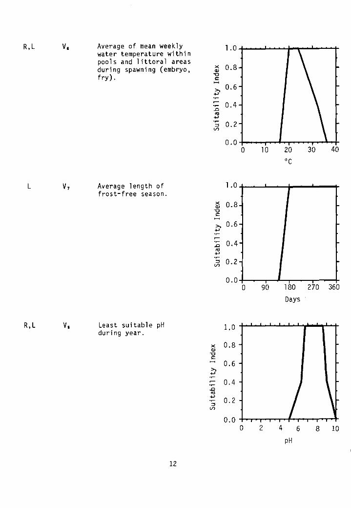
R,L V, Average of mean weekly 1.0water temperature withinpools and littoral areasduring spawning (embryo, x 0.80)

fry) . "'0c:......>, 0.6+J.,....r- 0.4.,......cttl

+J.,....0.2::l

V')

0.0a 10 20 30 40

°C

L V7 Average length of 1.0frost-free season.

x 0.8-0)"'0c:......e-, 0.6 -+J.,....r-.,.... 0.4..cttl+J.,....

0.2 -::lV')

0.0 JT

a 90 180 270 360

Days

R,L VI Least suitable pH 1,0during year.

x 0.80)

"'0c:...... 0.6>,+J

r- 0.4..cttl+J

0.2::l

V')

0.0a 2 4 6 8 10

pH

12

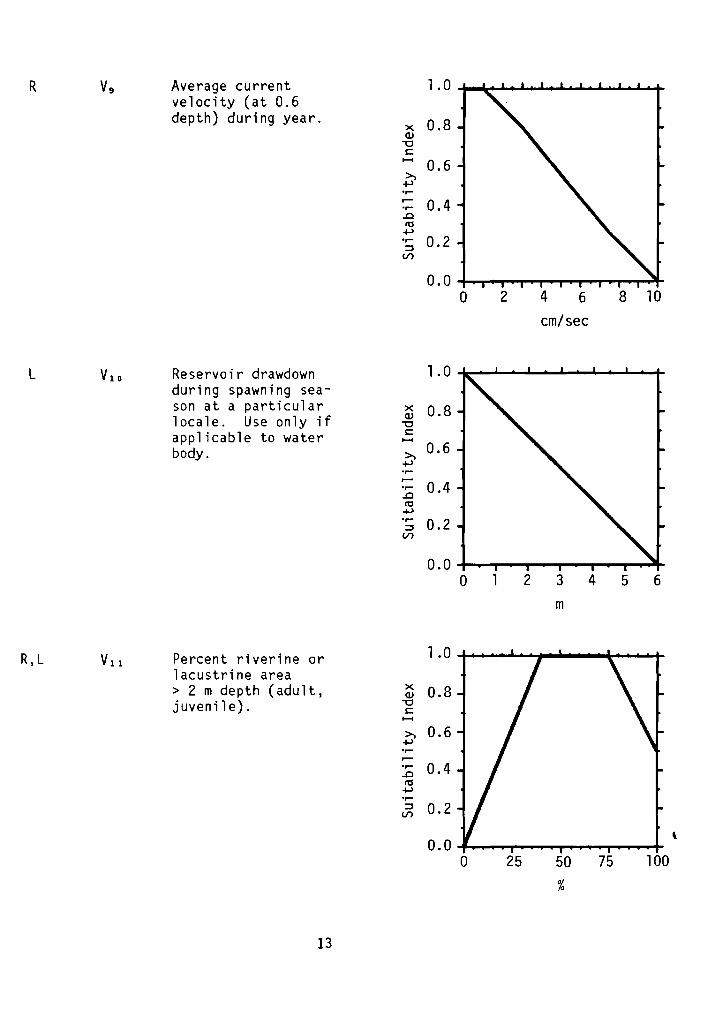
R V, Average current 1.0velocity (at 0.6depth) during year.

x 0.8<U"0C...... 0.6>,~.......... 0.4......0ro~..... 0.2~V)

0.00 2 4 6 8 10

em/sec

L VlO Reservoir drawdown 1.0during spawning sea-son at a particular x 0.8locale. Use only if <U

"0

applicable to water c......body. >, 0.6

~..........0.4.....

.0ro~..... 0.2~V)

0.00 2 3 4 5 6

m

R,L VII Percent riverine 1.0orlacustrine area> 2 m depth (adult, x 0.8<Ujuvenile). "0

c......>, 0.6~............... 0.4.0ro~.....~ 0.2V)

0.0,

0 25 50 75 100

%

13

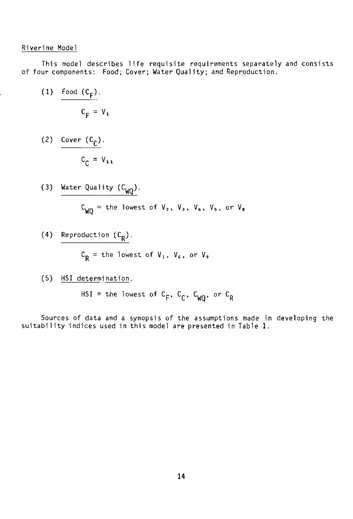
Riverine Model

This model describes life requisite requirements separately and consistsof four components: Food; Cover; Water Quality; and Reproduction.

(1) Food (CF)·

CF = VI

(2) Cover (CC).

Cc = VII

(3) Water Quality (CWQ).

CWQ = the lowest of V2 , V3 , V4 , v«. or Va

(4 ) Reproduction (CR).

CR = the lowest of VI' V6 , or v,

(5 ) HSI determination.

HSI = the lowest of CF' CC' CWQ' or CR

Sources of data and a synopsis of the assumptions made in developing thesuitability indices used in this model are presented in Table 1.

14

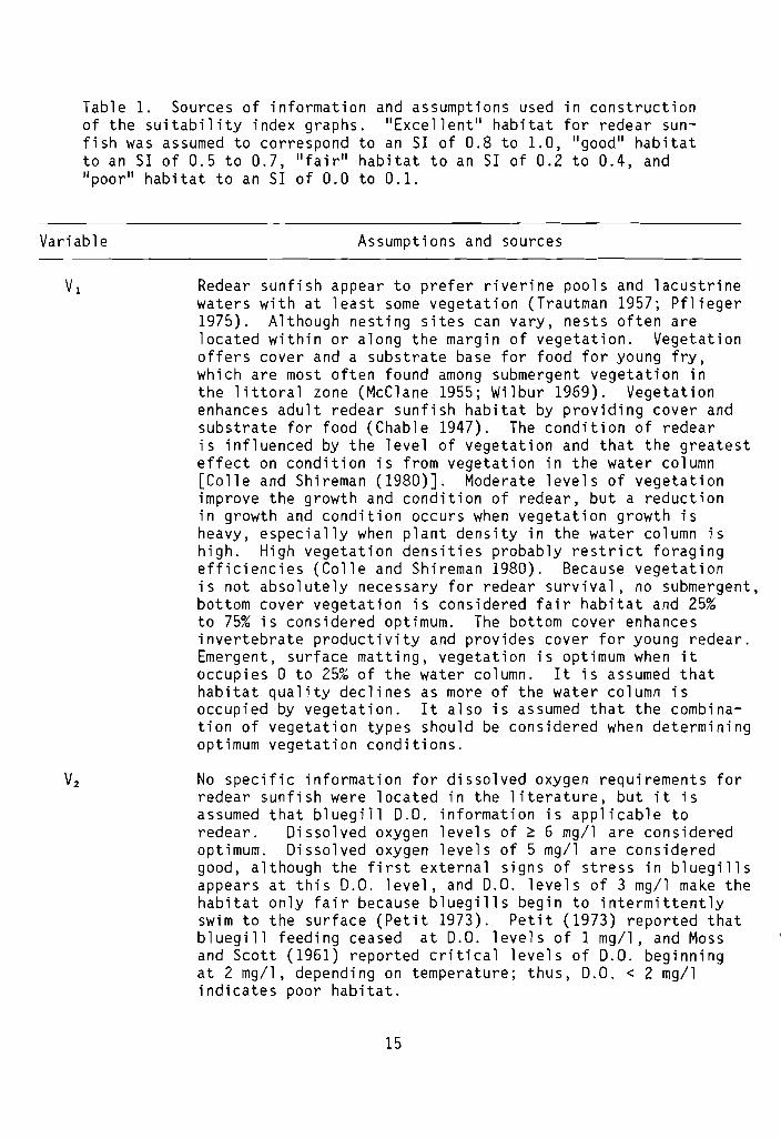
Table 1. Sources of information and assumptions used in constructionof the suitability index graphs. "Excellent" habitat for redear sun­fish was assumed to correspond to an SI of 0.8 to 1.0, "good" habitatto an SI of 0.5 to 0.7, "fair" habitat to an SI of 0.2 to 0.4, and"poor" habitat to an SI of 0.0 to 0.1.

Variable Assumptions and sources

Redear sunfish appear to prefer riverine pools and lacustrinewaters with at least some vegetation (Trautman 1957; Pflieger1975). Although nesting sites can vary, nests often arelocated within or along the margin of vegetation. Vegetationoffers cover and a substrate base for food for young fry,which are most often found among submergent vegetation inthe littoral zone (McClane 1955; Wilbur 1969). Vegetationenhances adult redear sunfish habitat by providing cover andsubstrate for food (Chable 1947). The condition of redearis influenced by the level of vegetation and that the greatesteffect on condition is from vegetation in the water column[Colle and Shireman (1980)J. Moderate levels of vegetationimprove the growth and condition of redear, but a reductionin growth and condition occurs when vegetation growth isheavy, especially when plant density in the water column ishigh. High vegetation densities probably restrict foragingefficiencies (Colle and Shireman 1980). Because vegetationis not absolutely necessary for redear survival, no submergent,bottom cover vegetation is considered fair habitat and 25%to 75% is considered optimum. The bottom cover enhancesinvertebrate productivity and provides cover for young redear.Emergent, surface matting, vegetation is optimum when itoccupies 0 to 25% of the water column. It is assumed thathabitat quality declines as more of the water column isoccupied by vegetation. It also is assumed that the combina­tion of vegetation types should be considered when determiningoptimum vegetation conditions.

No specific information for dissolved oxygen requirements forredear sunfish were located in the literature, but it isassumed that bluegill D.O. information is applicable toredear. Dissolved oxygen levels of ~ 6 mg/l are consideredoptimum. Dissolved oxygen levels of 5 mg/l are consideredgood, although the first external signs of stress in bluegillsappears at this D.O. level, and D.O. levels of 3 mg/l make thehabitat only fair because bluegills begin to intermittentlyswim to the surface (Petit 1973). Petit (1973) reported thatbluegill feeding ceased at D.O. levels of 1 mg/l, and Mossand Scott (1961) reported critical levels of D.O. beginningat 2 mg/l, depending on temperature; thus, D.O. < 2 mg/lindicates poor habitat.

15

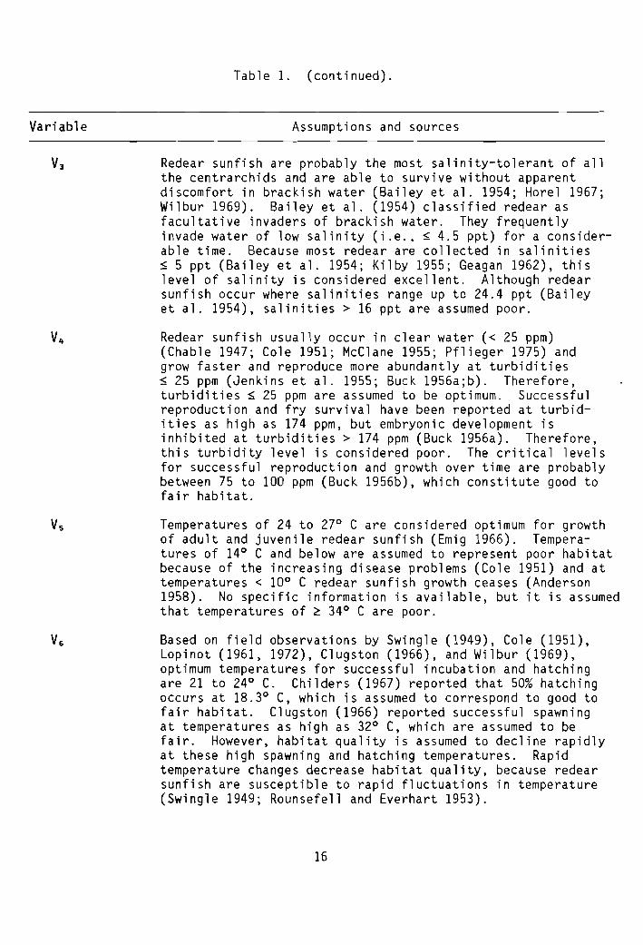
Table 1. (continued).

Variable Assumptions and sources

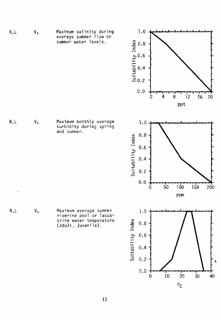
Redear sunfish are probably the most salinity-tolerant of allthe centrarchids and are able to survive without apparentdiscomfort in brackish water (Bailey et al. 1954; Horel 1967;Wilbur 1969). Bailey et al. (1954) classified redear asfacultative invaders of brackish water. They frequentlyinvade water of low salinity (i.e .. ~ 4.5 ppt) for a consider­able time. Because most redear are collected in salinities~ 5 ppt (Bailey et al. 1954; Kilby 1955; Geagan 1962), thislevel of salinity is considered excellent. Although redearsunfish occur where salinities range up to 24.4 ppt (Baileyet al. 1954), salinities> 16 ppt are assumed poor.

Redear sunfish usually occur in clear water « 25 ppm)(Chable 1947; Cole 1951; McClane 1955; Pflieger 1975) andgrow faster and reproduce more abundantly at turbidities~ 25 ppm (Jenkins et al. 1955; Buck 1956a;b). Therefore,turbidities ~ 25 ppm are assumed to be optimum. Successfulreproduction and fry survival have been reported at turbid­ities as high as 174 ppm, but embryonic development isinhibited at turbidities> 174 ppm (Buck 1956a). Therefore,this turbidity level is considered poor. The critical levelsfor successful reproduction and growth over time are probablybetween 75 to 100 ppm (Buck 1956b), which constitute good tofair habitat.

Temperatures of 24 to 27° C are considered optimum for growthof adult and juvenile redear sunfish (Emig 1966). Tempera­tures of 14° C and below are assumed to represent poor habitatbecause of the increasing disease problems (Cole 1951) and attemperatures < 10° C redear sunfish growth ceases (Anderson1958). No specific information is available, but it is assumedthat temperatures of ~ 34° C are poor.

Based on field observations by Swingle (1949), Cole (1951),Lopinot (1961, 1972), Clugston (1966), and Wilbur (1969),optimum temperatures for successful incubation and hatchingare 21 to 24° C. Childers (1967) reported that 50% hatchingoccurs at 18.3° C, which is assumed to correspond to good tofair habitat. Clugston (1966) reported successful spawningat temperatures as high as 32° C, which are assumed to befair. However, habitat quality is assumed to decline rapidlyat these high spawning and hatching temperatures. Rapidtemperature changes decrease habitat quality, because redearsunfish are susceptible to rapid fluctuations in temperature(Swingle 1949; Rounsefell and Everhart 1953).

16

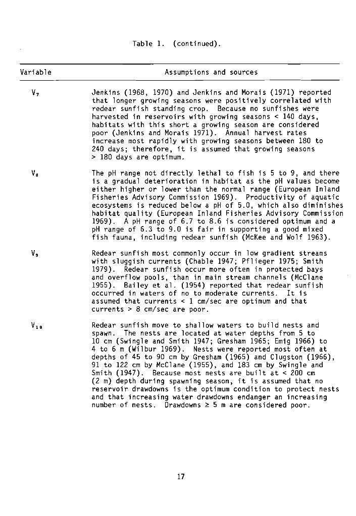
Table 1. (continued).

Variable Assumptions and sources

V7

V.

Jenkins (1968, 1970) and Jenkins and Morais (1971) reportedthat longer growing seasons were positively correlated withredear sunfish standing crop. Because no sunfishes wereharvested in reservoirs with growing seasons < 140 days,habitats with this short a growing season are consideredpoor (Jenkins and Morais 1971). Annual harvest ratesincrease most rapidly with growing seasons between 180 to240 days; therefore, it is assumed that growing seasons> 180 days are optimum.

The pH range not directly lethal to fish is 5 to 9, and thereis a gradual deterioration in habitat as the pH values becomeeither higher or lower than the normal range (European InlandFisheries Advisory Commission 1969). Productivity of aquaticecosystems is reduced below a pH of 5.0, which also diminisheshabitat quality (European Inland Fisheries Advisory Commission1969). A pH range of 6.7 to 8.6 is considered optimum and apH range of 6.3 to 9.0 is fair in supporting a good mixedfish fauna, including redear sunfish (McKee and Wolf 1963).

Redear sunfish most commonly occur in low gradient streamswith sluggish currents (Chable 1947; Pflieger 1975; Smith1979). Redear sunfish occur more often in protected baysand overflow pools, than in main stream channels (McClane1955). Bailey et al. (1954) reported that redear sunfishoccurred in waters of no to moderate currents. It isassumed that currents < 1 cm/sec are optimum and thatcurrents> 8 cm/sec are poor.

Redear sunfish move to shallow waters to build nests andspawn. The nests are located at water depths from 5 to10 cm (Swingle and Smith 1947; Gresham 1965; Emig 1966) to4 to 6 m (Wilbur 1969). Nests were reported most often atdepths of 45 to 90 cm by Gresham (1965) and Clugston (1966),91 to 122 cm by McClane (1955), and 183 cm by Swingle andSmith (1947). Because most nests are built at < 200 cm(2 m) depth during spawning season, it is assumed that noreservoir drawdowns is the optimum condition to protect nestsand that increasing water drawdowns endanger an increasingnumber of nests. Drawdowns ~ 5 m are considered poor.

17

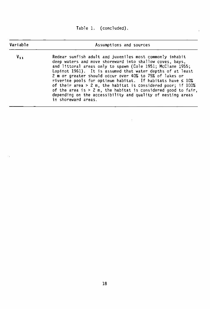
Table 1. (concluded).

Variable Assumptions and sources

Redear sunfish adult and juveniles most commonly inhabitdeep waters and move shoreward into shallow coves, bays,and littoral areas only to spawn (Cole 1951; McClane 1955;Lopinot 1961). It is assumed that water depths of at least2 m or greater should occur over 40% to 75% of lakes orriverine pools for optimum habitat. If habitats have ~ 10%of their area> 2 m, the habitat is considered poor; if 100%of the area is > 2 m, the habitat is considered good to fair,depending on the accessibility and quality of nesting areasin shoreward areas.

18

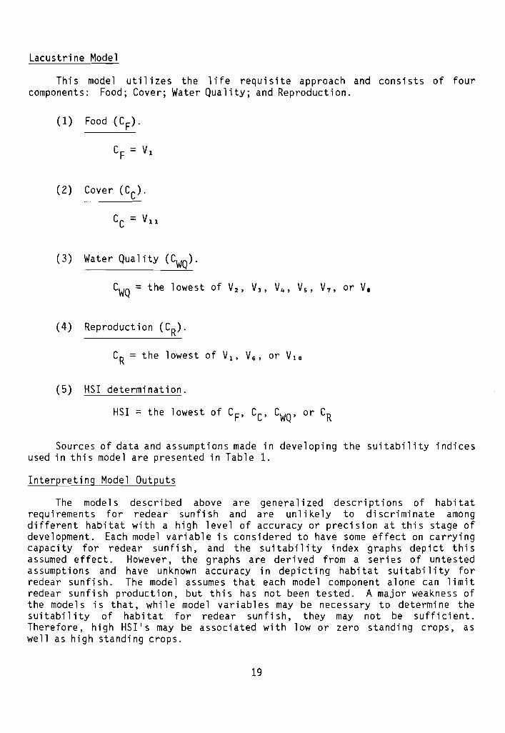
Lacustrine Model

This model utilizes the life requisite approach and consists of fourcomponents: Food; Cover; Water Quality; and Reproduction.

(2) Cover (CC).

(3) Water Quality (CWQ).

(4) Reproduction (CR).

(5) HSI determination.

HSI = the lowest of CF' CC' CWQ' or CR

Sources of data and assumptions made in developing the suitability indicesused in this model are presented in Table 1.

Interpreting Model Outputs

The models described above are generalized descriptions of habitatrequirements for redear sunfish and are unlikely to discriminate amongdifferent habitat with a high level of accuracy or precision at this stage ofdevelopment. Each model variable is considered to have some effect on carryingcapaci ty for redea r sunfi sh, and the sui tabi 1i ty index graphs dep i ct thi sassumed effect. However, the graphs are derived from a series of untestedassumptions and have unknown accuracy in depicting habitat suitability forredear sunfish. The model assumes that each model component alone can limitredear sunfish production, but this has not been tested. A major weakness ofthe models is that, while model variables may be necessary to determine thesuitability of habitat for redear sunfish, they may not be sufficient.Therefore, high HSI's may be associated with low or zero standing crops, aswell as high standing crops.

19

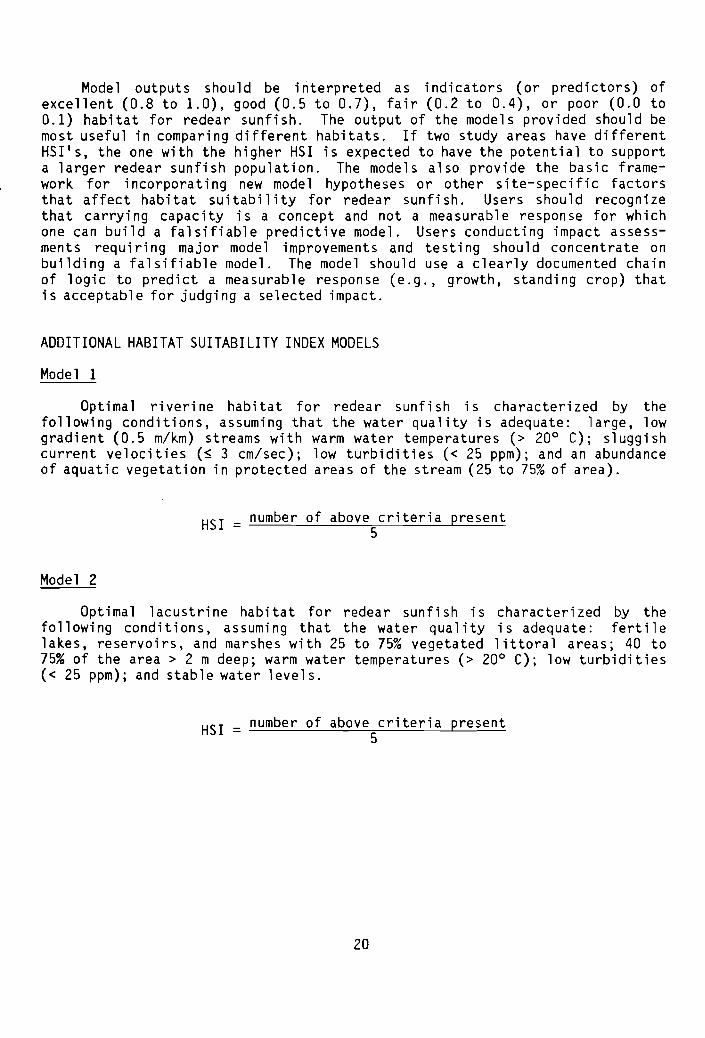
Model outputs should be interpreted as indicators (or predictors) ofexcellent (0.8 to 1.0), good (0.5 to 0.7), fair (0.2 to 0.4), or poor (0.0 to0.1) habitat for redear sunfish. The output of the models provided should bemost useful in comparing different habitats. If two study areas have differentHSI's, the one with the higher HSI is expected to have the potential to supporta larger redear sunfish population. The models also provide the basic frame­work for incorporating new model hypotheses or other site-specific factorsthat affect habitat suitability for redear sunfish. Users should recognizethat carrying capacity is a concept and not a measurable response for whichone can build a falsifiable predictive model. Users conducting impact assess­ments requiring major model improvements and testing should concentrate onbuilding a falsifiable model. The model should use a clearly documented chainof logic to predict a measurable response (e.g., growth, standing crop) thatis acceptable for judging a selected impact.

ADDITIONAL HABITAT SUITABILITY INDEX MODELS

Modell

Optimal riverine habitat for redear sunfish is characterized by thefollowing conditions, assuming that the water quality is adequate: large, lowgradient (0.5 m/km) streams with warm water temperatures (> 20° C); sluggishcurrent velocities (~ 3 em/sec); low turbidities « 25 ppm); and an abundanceof aquatic vegetation in protected areas of the stream (25 to 75% of area).

Model 2

HSI = number of above criteria present5

Optimal lacustrine habitat for redear sunfish is characterized by thefollowing conditions, assuming that the water quality is adequate: fertilelakes, reservoirs, and marshes with 25 to 75% vegetated littoral areas; 40 to75% of the area> 2 m deep; warm water temperatures (> 20° C); low turbidities« 25 ppm); and stable water levels.

HSI = number of above criteria present5

20

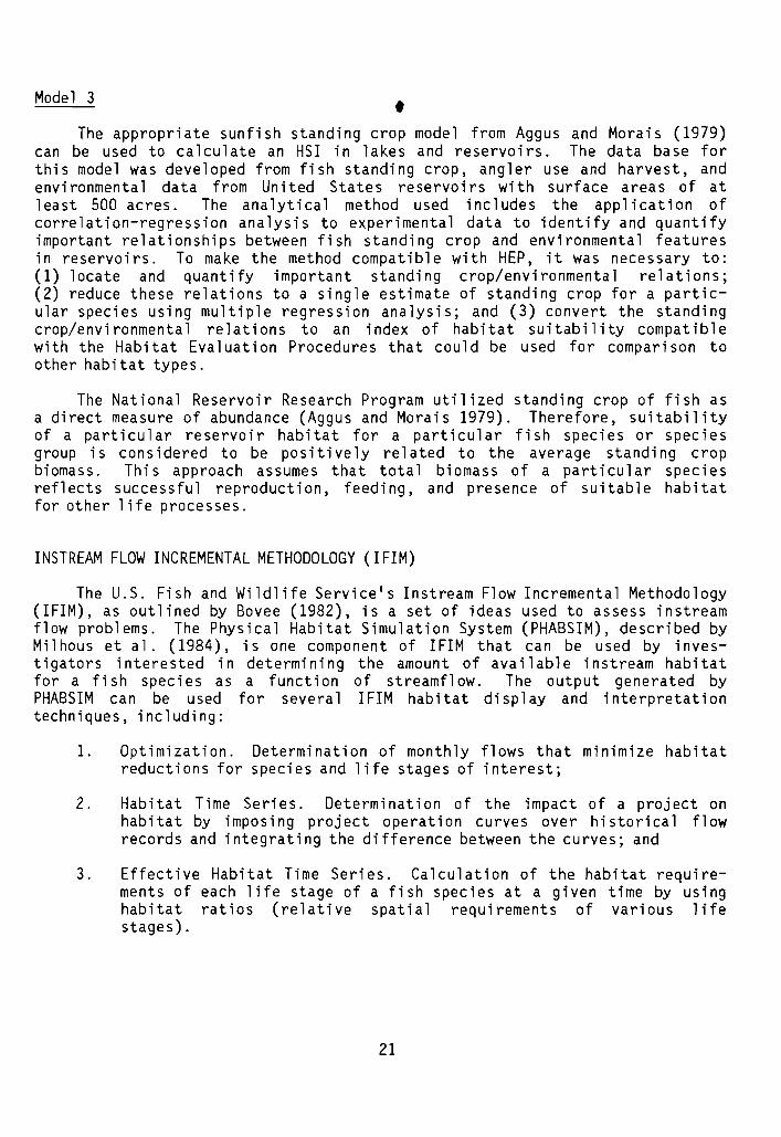
Model 3 •The appropriate sunfish standing crop model from Aggus and Morais (1979)

can be used to calculate an HSI in lakes and reservoirs. The data base forthis model was developed from fish standing crop, angler use and harvest, andenvironmental data from United States reservoirs with surface areas of atleast 500 acres. The analytical method used includes the application ofcorrelation-regression analysis to experimental data to identify and quantifyimportant relationships between fish standing crop and environmental featuresin reservoirs. To make the method compatible with HEP, it was necessary to:(1) locate and quantify important standing crop/environmental relations;(2) reduce these relations to a single estimate of standing crop for a partic­ular species using multiple regression analysis; and (3) convert the standingcrop/environmental relations to an index of habitat suitability compatiblewith the Habitat Eva 1uat i on Procedures that coul d be used for compari son toother habitat types.

The National Reservoir Research Program utilized standing crop of fish asa direct measure of abundance (Aggus and Morais 1979). Therefore, suitabilityof a particular reservoir habitat for a particular fish species or speciesgroup is considered to be positively related to the average standing cropbiomass. This approach assumes that total biomass of a particular speciesreflects successful reproduction, feeding, and presence of suitable habitatfor other life processes.

INSTREAM FLOW INCREMENTAL METHODOLOGY (IFIM)

The U.S. Fish and Wildlife Service's Instream Flow Incremental Methodology(IFIM), as outlined by Bovee (1982), is a set of ideas used to assess instreamflow problems. The Physical Habitat Simulation System (PHABSIM), described byMi 1hous et a1. (1984), is one component of I FIM that can be used by i nves­tigators interested in determining the amount of available instream habitatfor a fish species as a function of streamflow. The output generated byPHABSIM can be used for several IFIM habitat display and interpretationtechniques, including:

1. Optimization. Determination of monthly flows that minimize habitatreductions for species and life stages of interest;

2. Habi tat Ti me Seri es. Determi nat i on of the impact of a proj ect onhabitat by imposing project operation curves over historical flowrecords and integrating the difference between the curves; and

3. Effective Habitat Time Series. Calculation of the habitat require­ments of each life stage of a fish species at a given time by usinghabitat ratios (relative spatial requirements of various lifestages).

21

Suitability Index Graphs as Used in IFIM

PHABSIM utilizes Suitability Index graphs (SI curves) that describe theinstream suitability of the habitat variables most closely related to streamhydraulics and channel structure (velocity, depth, substrate, temperature, andcover) for each major life stage of a given fish species (spawning, egg incuba­tion, fry, juvenile, and adult). The specific curves required for a PHABSIManalysis represent the hydraulic-related parameters for which a species orlife stage demonstrates a strong preference (i .e., a species that only showspreferences for velocity and temperature will have very broad curves fordepth, substrate, and cover).

Four ca tegori es of SI curves are descri bed below. All speci es curvesfor HEP and IFIM are referred to collectively as suitability index (SI) curvesor graphs. The designation of a curve as belonging to a particular categorydoes not imply that there are differences in the quality or accuracy of curvesamong the four categories.

Category one curves are the most common type presently available for usewith HEP or IFIM. Usually category one curves have as their basis one or moreliterature sources. Some SI curves may be derived from general statementsmade in the literature about fishes (i.e., rainbow trout spawn in gravel; fryprefer shallow water). Some category one curve s may come from 1iteraturesources which include variable amounts of field data (i .e., from a sample sizeof 300, fry were observed in velocities ranging 0.0 to 3.0 ft/sec, and 80%were found in velocities less than 1.0 ft/sec). Other category one curves maybe based entirely on professional opinion, by using the Delphi technique oreducated guesswork (i.e., an expert believes that velocities ranging 1.0 to8.0 ft/sec are necessary for successful spawning of striped bass). Mostcategory one curves are the result of a combination of sources; the finalcurve may include information from the literature, combined with field data,and smoothed or modified using professional judgement. Category one curvesusua lly are intended to refl ect genera 1 habitat suitabi 1i ty throughout theentire geographic range of the species and throughout the year, unless theyare identified as being applicable only to a given area or season. In thelatter case, curves developed for a specific area or stream may not accuratelyreflect habitat utilization in other areas. Curves meant to describe thegeneral habitat suitability of a variable throughout the entire range of aspecies may not be as sensitive to small changes of the variable within aspecific stream (i.e., rainbow trout will generally utilize silt, sand, gravel,and cobble for spawning substrate, but utilize only cobble in Willow Creek,Co lorado).

Category two curves are derived from frequency analyses of field data,and are basically curves fit to a frequency histogram. Each curve describesthe observed utilization of a habitat variable by a life stage. Category twocurves unaltered by professional judgement or other sources of information arereferred to as utilization curves. When modified by judgement they thenbecome category one curves. Utilization curves from one set of data are notapplicable for all streams and situations (i.e., a depth utilization curvefrom a shallow stream cannot be used for the Missouri River). Category two

22

curves, therefore, are usually biased because of limited habitat availability.An ideal study stream would have all substrate and cover types present inequal amounts; all depth, velocity, and percent cover intervals available inequal proportions; and all combinations of all variables in equal proportions.Utilization curves from such a perfectly designed study theoretically shouldbe transferabl e to any stream withi n the geographi ca 1 range of the speci es.Curves from streams with high habitat diversity, then, are generally moretransferable than curves from streams with low habitat diversity. Users of acategory two curve should first review the stream description to see if condi­tions are similar to those present in the stream segment to be investigated.Some variables to consider might include stream width, depth, discharge,gradient, elevation, latitude and longitude, temperature, water quality,substrate and cover diversity, fish species associations, and data collectiondescriptors (time of day, season of year, sample size, sampling methods). Ifone or more deviate significantly from those of the proposed study site, thencurve transference is not advised, and the investigator should develop his owncurves.

Category three curves are derived from utilization curves which have beencorrected for envi ronmenta 1 bi as and therefore represent preference of thespecies. To generate a preference curve, one must simultaneously collecthabitat utilization data and habitat availability data from the same area.Habitat availability should reflect the relative amount of different habitattypes in the same proportions as they exist throughout in the stream-studyarea. A curve is then developed for the habitat frequency distribution in thesame way as for fish utilization observations, and the equation coefficientsof the availability curve are subtracted from the equation coefficients of thethe utilization curve, resulting in preference curve coefficients. Theoret­i ca l ly , category three curves shoul d be uncondit i onally transferable to anystream, although this has not been validated. At present, very few categorythree curves exist because most habitat utilization data sets are withoutconcomitant habitat availability data sets. In the future, the need to collecthabitat availability data will be impressed upon investigators.

Category four curves (conditional preference curves), describe habitatrequirements as a function of interaction among variables. For example, fishdepth utilization may depend on the presence or absence of cover; or velocityutilization may depend on time of day or season of year. Category four curvesare just beginning to be developed by IFASG.

HSI models generally utilize category one curves for habitat evaluation.IFIM analyses may utilize any or all categories of curves, but category threeand four curves yield the most precise results in IFIM applications; andcategory two curves wi 11 yield accurate results if they are found to betransferable to the stream segment under investigation. If category twocurves are not felt to be transferable for a particular application, thencategory one curves may be a better choice.

23

For an 1F1M analysis of riverine habitat, an investigator may wish toutilize the curves available in this publication; modify the curves based onnew or additional information; or collect field data to generate new curves.For example, if an investigator has information that spawning habitat utiliza­tion in his study stream is different from that represented by the S1 curves,he may want to modify the existing S1 curves or collect data to generate newcurves. Once the curves to be used are decided upon, then the curve coordi­nates are used to build a computer file (F1SHF1L) which becomes a necessarycomponent of PHABS1M analyses (Milhous et al. 1984).

Availability of Graphs for Use in 1F1M

All the S1 curves available for the 1F1M analysis of redear sunfishriverine physical microhabitat are category one (Table 2), and can be found inthe HS1 model section of this report (sources and assumptions in Table 1).Some of the curves may require modification before use in the PHAB51M model.

Redea r sunfi sh genera lly spawn sometime between February and October,depending on locale, and spawning duration may range from 1 to 8 months(Carlander 1977). The 51 curves for spawning habitat should be used for thedefined spawning period within the selected study area. Egg incubationgenera lly requi res 1 to 2 days (Ib t d) and, therefore, egg i ncubat i on curvesshould be used for the defined spawning period. Fry are defined as individualsless than 1.0 inches in length, and fry curves should be used for the periodfrom 3 days after the beginning to 3 months after the end of spawning.Juveniles are defined to range in length from 1.0 to 6.0 inches; and sexuallymature adults are generally greater than 6.0 inches in length. Juvenile andadult habitat is required year-round.

The 51 curves for velocity and percent cover suitability (Vg ; VI) are

meant to be used for all 1i fe stages of redear sunfi sh. The 51 curve forspawning, egg incubation, and fry temperature suitability (V 6 ) above 20° C is

identical to that for juveniles and adults (V s ) . Curve coordinates can be

taken from the curves for entry into F15HF1L. Any curves which are thoughtnot to represent circumstances found at a given site may be modified for 1F1Mapplications. No curves are available for depth or substrate suitability forany of the 1ife stages. and will have to be generated by the investigatorbefore a complete 1F1M analysis can be undertaken.

24

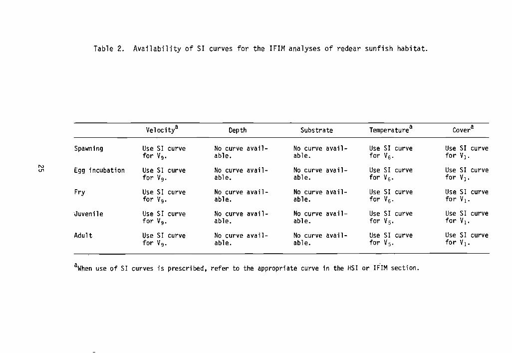
Table 2. Availability of S1 curves for the 1F1M analyses of redear sunfish habitat.

Velocitl Depth Substrate Temperaturea Covera

Spawning Use SI curve No curve avail- No curve avail- Use SI curve Use SI curvefor Vg. able. able. for V6' for Vi -

N Egg incubation Use SI curve No curve avail- No curve avail-U"I Use SI curve Use SI curvefor Vg • able. able. for V6' for VI'

Fry Use SI curve No curve avail- No curve ava il- Use SI curve Use SI curvefor Vg • able. able. for V6 • for VI'

Juvenile Use 51 curve No curve avail- No curve avail- Use SI curve Use SI curvefor Vg • able. able. for V5' for Vi-

Adult Use SI curve No curve avail- No curve avail- Use SI curve Use SI curvefor Vg. able. able. for V5' for Vi-

aWhen use of SI curves is prescribed. refer to the appropriate curve in the HSI or IFIM section.

REFERENCES

Aggus, L. R., and D. 1. Morais. 1979. Habitat suitability index equationsfor reservoirs based on standing crop of fish. Natl. Reservoir ResearchProgram. Report to U.S. Fish Wildl. Serv., Habitat Evaluation Proj., Ft.Co 11 ins, CO. 120 pp.

Anderson, R. O. 1958. A seasonal study of food consumption and growth of thebluegill. Abstr. Midwest Wildl. Conf. 20:5-6.

Bailey, R. M., H. E. Winn, and C. L. Smith. 1954. Fishes from the EscambiaRiver, Alabama and Florida, with ecologic and taxonomic notes. Proc.Acad. Nat. Sci., Philadelphia 106:109-164.

Beland, R. D. 1953. The occurrence of two additional centrarchids in thelower Colorado River. California Fish Game 39(1):149-151.

Bovee, K. D. 1982. A guide to stream habitat analysis using the InstreamFlow Incremental Methodology. Instream Flow Information Paper 12. U.S.Fish Wildl. Servo FWS/OBS-82/26. 248 pp.

Buck, D. H. 1956a. Effects of turbidity on fish and fishing. Oklahoma FishRes. Lab. Rep. 65. 62 pp.

1956b. Effects of turbidity on fish and fishing. Trans. N.Am. Wildl. Conf. 21:249-261.

Carl ander, K. D. 1977. Redear sunfi sh. Pages 124-131 in Handbook of fresh­water fishery biology. Iowa State Univ. Press, Ames. 431 pp.

Carothers, J. L., and R. Allison. 1968. Control of snails by the redear(shell cracker) sunfish. F.A.O. Fish. Rep. 44(5):399-406.

Chable, A. C. 1947. A study of the food habits and ecological relationshipsof sun-fishes of northern Florida. M.S. Thesis, Univ. Florida,Gainesville. 96 pp.

Childers, W. F. 1967. Hybridization of four species of sunfishes(Centrarchidae). Illinois Nat. Hist. Surv. Bull. 29(3):159-214.

Clugston, J. P. 1966. Centrarchid spawning in the Florida everglades.Q. J. Fla. Acad. Sci. 29(2):137-144.

Cole, V. W. 1951. Contributions to the life history of the redear sunfish(Lepomis microlophus) in Michigan waters. M.S. Thesis, Michigan StateColl., East Lansing. 54 pp.

Colle, D. E., and J. V. Shireman. 1980. Coefficients of condition for large­mouth bass, bluegill, and redear sunfish in Hydrilla-infested lakes.Trans. Am. Fish. Soc. 109:521-531.

26

Cowardin, L. M., V. Carter, F. C. Golet, and E. T. LaRoe. 1979. Classifica­tion of wetlands and deepwater habitats of the United States. U.S. FishWildl. Servo FWS/OBS-79/31. 103 pp.

Dineen, W. J. 1968. Determination of the effects of fluctuating water levelson the fish population of Conservation Area III. Florida Game, FreshWater Fish Comm. D-J Proj. F-16; Job 1-E. 15 pp.

Emig, J. W. 1966. Red-ear sunfish. Pages 392-399 in A. Calhoun, ed. Inlandfi sheri es management. Ca 1Horn i a Fi sh Game Dept:-

European Inland Fisheries Advisory Commission Working Party on Water QualityCriteria for European Freshwater Fish. 1969. Water quality criteria forEuropean freshwater fi sh-extreme pH va1ues and in 1and fi sheri es. WaterRes. 3:593-611.

Finnell, J. C., R. M. Jenkins, and G. E. Hall. 1956. The fishery resourcesof the Little River System, McCurtain County, Oklahoma. Oklahoma Fish.Res. Lab. Rep. 55. 82 pp.

Geagan, D. W. 1962. An investigation of the sport fishes in the coastalwaters of Louisiana. Ninth Biennial Rep. Louisiana Wildl. FishComm. : 125-132.

Gresham, G. 1965. The Chinks are bedded. Outdoor Life 135(3):24-35, 86-90.

Hill, L. G., G. D. Schnell, and J. Pigg. 1975. Thermal acclimation andtemperature selection in sunfishes (Lepomis, Centrarchidae). SouthwesternNat. 20(2):177-184.

Horel, G. 1967. Fish population studies. Florida Fed. Aid Proj. F-21-2, Job1-A. Annu. Rep. 98 pp.

Hubbs, C. L., and K. F. Lagler. 1964. Fishes of the Great Lakes Region.Univ. Michigan Press, Ann Arbor. 213 pp.

Hui sh, M. T. 1957. Food habits of three Centrarchi dae in Lake George,Florida. Proc. Southeastern Game and Fish Comm. 11:293-302.

Jenkins, R. M. 1955. A summary of fish population studies conducted during1954 at Ardmore City Lake, String town Sub-prison Lake and Pawhuska CityLake. Oklahoma Fish. Res. Lab. Rep. 48. 31 pp.

1968. The influence of some environmental factors on standingcrop and harvest of fishes in U.S. reservoirs. Reservoir FisheryResources Symposium, April 5-7, 1967, Athens, GA 63:298-321.

1970. The influence of engineering design and operation andother environmental factors on reservoir fishery resources. J. Am. WaterResour. Assoc. Water Resour. Bull. 6(1):110-119.

27

1976. Prediction of fish production in Oklahoma Reservoirs onthe basis of environmental variables. Annu. Oklahoma Acad. Sci. 5:11-20.

Jenkins. R. M.,harvest inHa11, ed.Pub1. 8.

and D. 1. Mora is. 1971. Reservoi r sport fi shi ng effort andrelation to environmental variables. Pages 371-384 in G. E.Reservoir fisheries and limnology. Am. Fish. So~ Spec.

Jenkins. R., R. Elkin, and J. Finnell. 1955. Growth rates of six sunfishesin Oklahoma. Oklahoma Fish. Res. Lab. Rep. 59:1-46.

Kilby. J. D. 1955. The fishes of two gulf coastal marsh areas of Florida.Tulane Stud. Zool. 2(8):175-247.

Krumholz, L. A. 1950. New fish stocking policies for Indiana ponds. Proc.N. Amer. Wi1d1. Conf. 15:251-270.

Leidy. G. R., and R. M. Jenkins . .1977. The development of fishery compart­ments and population rate coefficients for use in reservoir ecosystemmodeling. U.S. Fish Wildl. Serv., Nat1. Reservoir Res. Program.Fayetteville, Arkansas. Contract Rep. Y-77-1. 225 pp.

l.opt not , A. 1961. The red-ear sunfish. Illinois Wild1. 17(1):3-4.

Lopinot, A. C. 1972. Pond fish and fishing in Illinois. Illinois Dept.Conserv. Fish. Bull. 5:62 pp.

McClane. W. W. 1955. The fishes of the St. Johns River Florida. Ph.D.Dissertation, Univ. Florida, Gainesville. pp. 243-249.

McKee, J. E., and H. W. Wolf. 1963. Water quality criteria, 2nd edition.Resources Agency of California. State Water Quality Control Board, Pub1.3-1. 548 pp.

Milhous, R. T., D. L. Wegner, and T. Waddle. 1984. User's guide to thePhysical Habitat Simulation System. Instream Flow Information Paper 11.U.S. Fish Wi1d1. Servo FWS/OBS-81/43 Revised.

Moss. D. D., and D. C. Scott. 1961. Dissolved-oxygen requirements of threespecies of fish. Trans. Am. Fish. Soc. 90(4):377-393.

Parks, C. E. 1949. The summer food of some game fishes of Wisiona Lake.Invest. Indiana Lakes, Streams 3(4):235-245. (Cited by Emig 1966).

Pasch, R. W. 1975. Status of the redear sunfish fishery in the Flint River.Georgia Dept. Nat. Resour., D-J Proj. F-28-2. 15 pp.

Petit, G. D. 1973. Effects of dissolved oxygen on survival and behavior ofselected fishes of western Lake Erie. Ohio Bio1. Surv. Bull. 4(4):1-76.

28

Pflieger, W. L. 1975. The fishes of Missouri. Missouri Dept. Conserv.342 pp.

Rounsefell, G. A., and W. H. Everhart. 1953. Fishery science, its methodsand applications. John Wiley and Sons, New York. 444 pp.

Schoffman, R. J. 1939. Age and growth of the red-eared sunfish in ReelfootLake. J. Tennessee Acad. Sci. 14(3):61-71.

Smith, P. W. 1979. The fishes of Illinois. Univ. Illinois Press. 314 pp.

Swingle, H. S. 1949. Some recent developments in pond management. Trans. N.Am. Wildl. Conf. 14:295-312.

Swingle, H. S., and E. V. Smith. 1947. Management of farm fish ponds.Alabama Polytechnic Inst., Agric. Exp. Stn. Bull. 254 (Part II). 30 pp.

Trautman, B. B. 1957. The fishes of Ohio. Ohio State Univ. Press. 683 pp.

Wilbur, R. L. 1969. The redear sunfish in Florida. Florida Game, FreshWater Fish Comm. Fish Bull. 5. 64 pp.

29

50272 -IlU

REPORT DOCUMENTATION : 1. REPORT NO. : 2. 3. RecIpient's AccelSion No.IPAGE FWS/OBS-82/10.79

4. TItle and Subtitle 5. Report DateHabitat Suitability Index Models and Instream Flow Suitability September 1984

Curves: Redear sunfish 6. --I 7. Author(s) bien beonart, U. l:.ugene nauqnen , xatn reen Iwomey , ana 8. Performinz Orllnizatlon Rept. No.Patrick C. Nelson

•

9. Perfo"";nl Orlanization Name and Addr... Instream Flow and Aquatic Systems Grou] 10. Projec:t/T..k/Work Unit No.~yoming Cooperative Western Energy and Land Use Team

Fishery Unit U.S. Fish and Wildlife Service 11. Contract(C) or Grant(Gl No.University of Wyoming 2627 Redwing Road (ClLaramie, WY 82071 Ft. Collins, CO 80526-2899Oklahoma Coop. Fishery Research Unit, Oklahoma State Univ., Stillwa t~lr, OK 74074

12.SponIOrinIOrpnlzatlonName.ndAdd,...WeStern Energy and Land Use Team 13. Type of Report & Period CoveredDivision of Biological ServicesResearch and DevelopmentFish and Wildlife Service 14.

U.S. Depa rtrnent of the Interi or15. Supplememary Not..

. II. Abctree:t (Umlt: 200 word.)

Washington, DC 20240

The habitat suitability index (HSI) models presented in this publication aid inidentifying important habitat variables for the redear sunfish (Lepomis microlophus).Information obtained from the research literature and expert reviews are synthesizedinto models which present hypotheses of species-habitat relationships.

A brief discussion of using selected Suitability Index (SI) curves from HSI modelsas a component of the Instream Flow Incremental Methodology (IFIM) is provided.Additional SI curves, specifically designed for analysis of Redear sunfish habitatwith IFIM, are also presented.

17. Document Analysl. a. DescriptorsFishesHabitabilityMathematical modelsAquatic biology

b. Identlfiers/Open·Ended TermlRedear sunfishLepomis microlophusHabitat suitabilityInstream Flow Incremental Methodology

c. COIATl FIeld/Group

i

Ii

I

II. Availability Statement

Release unlimited

(s.. AHSt-Dt.ll)'il'U.s. GOVERNMENT PRINTING OFFICE: 1984-781-455/9548

i Ii. Security CI... (This Report)i Unclassified: 20. Security cr... (T!'is .Pe"e': UnclaSSlfleas.. In.tructlon. on Reverse OPTIONAL FOR.. 272 (4-77)

(Fo""erly NTIS-351O."artment of Commen:1t

......,- . .. ..~

""

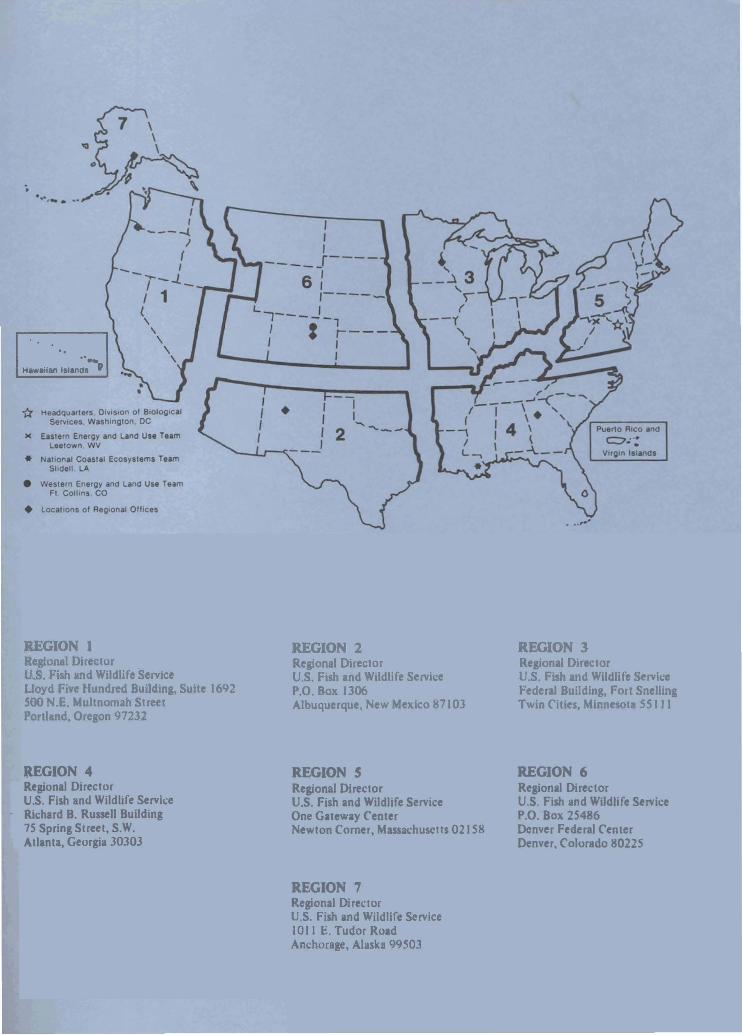
* Headquarters , 0lvI5 10n Of Biolog icalservices . Wasn,ngton . DC

)( Eastern Energy and Land Use TeamLeerown. WV

* Naloonal Coastal Ecosystems TeamSlide ll LA

• Western Energy aM LaM Use TeamFI ccu.ns. CO

• Locat ions of RegIonal Ollices

UGION 1Rqiunlll DirectorO.S. Fish lind Wildlife ServiceUoyd Five Hundred Building, Suite 1692500N.E. Multnomah StreetPortland, Oregon 97232

REGION 4Regional DirectorU.S. Fish and Wildlife ServiceRichard B. Russell Building75 Spring Street, S.W.Atlanta, Georgia 30303

,,I__r----

6!,-----L, J_1, : ,---

I ,I

REGION 2Regional DirectorU.S. Fish and Wildlife ServiceP.O. Box 1306Albuquerque, New Mexico 87103

REGION SRegional DirectorU.S. Fish and Wildlife ServiceOne Gateway CenterNewton Comer, Massachusetts 02158

REGION 7Regional DirectorU.S. Fish and Wildlife Service10II E. Tudor RoadAnchorage, Alaska 99503

,."

REGION 3Regional DirectorU.S. Fish and Wildlife ServiceFederal Building, Fort SnellingTwin Cities, Minnesota 5SIII

REGION 6Regional DirectorU.S. Fish and Wildlife ServiceP.O. Box 25486Denver Federal CenterDenver, Colorado 80225

DEPARTMENT OF THE INTERIORu.s. FISH AND WILDLIFE SERVICE

As the Nation's principal conservation asency, the Department of the Interior has respon­sibility for most of our .nationally owned public lands and natural resources. This includesfosterins the wisest use of our land and water resources, protecting our fish and wildlife,preserving th.environmental and cultural'values of our national parks and historical places,and providing for the enjoyment of life throulh outdoor recreation. The Department as­sesses our energy and mineral resources and works to assure that their development is inthe best interests of all our people. The Department also has a major responsibility forAmerican Indian reservation communities and for people who live in island territories underU.S. administration.