Embed Size (px)
Citation preview

Study and Interpretation of the Millimeter-wave Spectrum of
Venus
By
Antoine K. Fahd
Paul G. Steffes, Principal Investigator
School of Electrical Engineering
Georgia Institute of Technology
Atlanta, GA. 30332-0250
(404) 894-3128
June, 1992
Technical Report No. 1992-1
Prepared under NASA grant NAGW-533
_t: Tr17 MiLLT_CT: -_AV_ ._P[CTi_L]M L;r V;
T_;chnic:_! _:',e)ort No. ]992-1 (Georgi-/ Inst.of r(,<:i.) 17_ _ CSCL 03P
_3/_1
t_9 Z-25Z_? 0
Uncl ,_s
O0 91 Z 3 l
https://ntrs.nasa.gov/search.jsp?R=19920016037 2018-08-28T18:46:02+00:00Z

Study and Interpretation of the Millimeter-wave Spectrum of
Venus
APPROVED
Professor P s, Chairperson
/_rofessor A.$1 Gasfewski
- Professor W. Scott
Date Approved by Chairperson 3//0/7 2"--
ii

ACKNOWLEDGMENTS
I am grateful to my advisor, Dr. P.G. Steffes for his
guidance, support and patience. I thank the following faculty
members for their time and careful examination of this
document: Dr. A.J. Gasiewski (reader), Dr. W. Scott (reader),
Dr. R. Callen (chairman of the qualifying and proposal
committees) and Dr. C. G. Justus.
I thank the following individuals for their contributions
to this work: Dr. D.P. Campbell, Mr. J.J. Gallagher
(deceased), Dr. R. Moore, and Mr. S. Halpbern of the Georgia
Tech Research Institute (GTRI); Dr. T.E. Brewer and Dr. A.
Gasiewski (Georgia Tech-School of E.E.), for their generous
assistance with the laboratory equipment and for providing
illuminating discussion. I also thank Dr. I. dePater
(Berkeley), and Dr. T.R. Spilker (JPL) for their comments and
helpful suggestions.
I would also like to thank my family and friends who gave
me support and encouragement through my tenure as a graduate
student: Kozhaya (deceased), Antoinette, Michael and Joumana
Fahd, Milia and Fady Garabet, Mary Rashid and the rest of the
Fahd and Khairallah families. I also thank Robert Troxler,
Joanna Joiner, and Jon Jenkins.
iii

This work was supported by the Planetary Atmospheres
Program of the National Aeronautics and Space Administration
under grant NAGW-533.
iv
O
TABLE OF CONTENTS
ACKNOWLEDGMENTS .................... iii
TABLE OF CONTENTS ................... v
LIST OF FIGURES .................... ix
LIST OF TABLES .................... xvii
SUMMARY ....................... xviii
CHAPTER I ....................... 1
INTRODUCTION ................... 1
i.i Background and Motivation ........ 1
1.2 Organization .............. 4
CHAPTER 2 .......................
MICROWAVE AND MILLIMETER-WAVE OPACITY OF GASEOUS
SULFUR DIOXIDE (SO2) UNDER VENUS-LIKE
CONDITIONS .................
6
v

2.1 Motivation for Experiment ........
2.2 Experimental Approach ..........
2.2.1 Microwave Configuration .....
2.2.2 Millimeter-Wave Configuration
2.3 Determination of the Absorptivity of SO 2
2.4 Experimental Uncertainties .......
2.5 Experimental Results and Theoretical
Characterization of the SO 2 Opacity • •
6
8
8
12
15
20
23
CHAPTER 3 .......................
LABORATORY MEASUREMENTS OF THE OPACITY OF LIQUID
SULFURIC ACID AT MILLIMETER WAVELENGTHS . •
3.1 Motivation for Experiment ........
3.2 Experimental approach ..........
3.2.1 Experimental Procedure ......
3.2.2 Determination of the Dielectric
Constants .............
3.3 Experimental Results ..........
3.4 Theoretical Characterization of the
Dielectric Constant of Liquid Sulfuric
Acid (H2SO_) at Millimeter-Wavelengths
32
32
32
34
37
39
42
46
CHAPTER 4 ......................
VAPOR PRESSURE OF GASEOUS SULFURIC ACID (H2SO4) •
4.1 Introduction and Motivation .......
vi
54
54
54

4.2 Application of the Measured Vapor
Pressure of H2SO4 to the Atmosphere of
Venus ................. 57
CHAPTER 5 .......................
MEASUREMENT OF THE OPACITY OF GASEOUS SULFURIC
ACID (H2SO4) AT W-BAND ...........
5.1 Motivation ...............
5.2 Laboratory Configuration ........
5.2.1 Measurement Procedure ......
5.3 Experimental Uncertainties .......
5.4 Experimental Results and Theoretical
Characterization of H2SO 4 Absorption .
62
62
62
64
68
69
72
CHAPTER 6 .......................
MODELING OF THE ATMOSPHERE OF VENUS .......
6.1 Development of the Radiative Transfer
Model .................
6.2 Disk Average Brightness .........
6.3 Parameters of the Radiative Transfer
Model .................
6.3.1 Pressure-Temperature Profile of
Venus ...............
6.3.2 Gaseous CO 2 Absorption ......
6.3.3 S02-C02 Absorption ........
vii
79
79
79
83
84
85
85
87

6.3.4 Liquid Sulfuric Acid Condensates . 90
6.3.4.1 Scattering Effects of the
Cloud Condensates ...... 96
6.3.5 Gaseous H2SO_-CO 2 Absorption . . . i00
6.3.6 H20 Vapor ............ i01
6.4 Modeling Results ............ 105
CHAPTER 7 ....................... 123
SUMMARY AND CONCLUSIONS ............. 123
7.1 Uniqueness of Work ........... 123
7.2 Suggestion for Future Work ....... 127
APPENDIX A ..................... 130
A.I Measurement of the Vapor Pressure of Sulfuric
Acid .................... 130
A.2 Determination of the Dissociation Factor and
the Partial Pressure of Gaseous Sulfuric Acid
(H2SO4) ................... 135
A.3 Measurement Results ............. 140
BIBLIOGRAPHY ..................... 154
viii

LIST OF FIGURES
Figure 2.1 Block diagram of Georgia Tech Spectrometer,
as configured for measurements of microwave
refraction and absorption of gases under simulated
Venus conditions .................
Figure 2.2 Block diagram of the millimeter-wave setup
for measuring the absorption coefficient of
gaseous sulfur dioxide (SO2) under Venus-like
conditions ....................
Figure 2.3 Sketch of the Fabry-Perot resonator used in
the measurements of the absorption coefficient of
SO2/C02 at 94.1 GHz ................
Figure 2.4 Measured absorption coefficient (normalized
by mixing ratio) of gaseous SO2/CO 2 mixture at
2.24 GHz. Measurements were made at 296 K with an
SO 2 density of 8.33% ...............
Figure 2.5 Measured absorption coefficient (normalized
by mixing ratio) of gaseous S02/CO 2 mixture at
21.7 GHz. Measurements were made at 296 K with an
SO 2 density of 8.33% ..............
13
14
24
25
ix

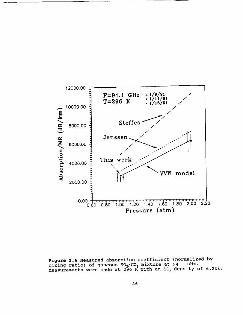
Figure 2.6 Measured absorption coefficient (normalized
by mixing ratio) of gaseous SO2/CO2 mixture at
94.1 GHz. Measurements were made at 296 K with an
SO 2 density of 6.25% ...............
Figure 2.7 Representations of the absorption of sulfur
dioxide at line centers ..............
Figure 3.1 Sketch of the free space measurement system
Figure 3.2 Sketch of the liquid cell used in the free
space measurement of the dielectric constant of
sulfuric acid ...................
Figure 3.3 Block diagram of the free space measurement
setup, as configured for measurements of the
millimeter wave complex dielectric constant of
liquid sulfuric acid .............
Figure 3.4 Detailed sketch of the liquid cell
representing various media and their respective
interfaces ....................
Figure 3.5 The measured real part of the complex
dielectric constant of water and sulfuric acid for
frequencies between 30 and 40 GHz at room
temperature. Error bars indicate ±Io about the
mean .....................
Figure 3.6 The measured imaginary part of the complex
dielectric constant of water and sulfuric acid for
frequencies between 30 and 40 GHz at room
x
26
27
35
36
38
40
43

temperature. Error bars indicate ±la about the
mean.......................
Figure 3.7 The measured real part of the complex
dielectric constant of water and sulfuric acid for
frequencies between 90 and i00 GHz at room
temperature. Error bars indicate ±la about the
mean.......................
Figure 3.8 The measured imaginary part of the complex
dielectric constant of water and sulfuric acid for
frequencies between 90 and i00 GHz at room
temperature. Error bars indicate ±la about the
mean.......................
Figure 3.9 Comparison between the measured and
calculated real part of the complex dielectric
constant of liquid sulfuric acid at room
temperature ....................
Figure 3.10 Comparison between the measured and
calculated imaginary part of the complex
dielectric constant of liquid sulfuric acid at
room temperature .................
Figure 4.1 Corrected measurements of the microwave
absorptivity of gaseous sulfuric acid at 2.24 GHz.
Solid line represents a best-fit multiplicative
expression for the absorptivity while the dashed
line is the original expression (Steffes, 1985).
xi
44
47
48
52
53
58

Figure 4.2 An abundance profile for gaseous sulfuric
acid in the atmosphere of Venus after Jenkins and
Steffes (1991). The dashed line represents
saturation abundance of gaseous H2SO4 in the
atmosphere of Venus ................
Figure 5.1 Block diagram of the atmospheric simulator
as configured for measurements of the millimeter-
wave absorption of gaseous H2SO_ under Venus
atmospheric conditions at 94.1 GHz........
Figure 5.2 Laboratory measurements of the normalized
absorptivity (dB/km) of gaseous H2SO4 in a CO 2
Atmosphere at 94.1 GHz. Solid curves are the
theoretically calculated absorption from the VVW
formalism .....................
Figure 5.3 Diagram of the peak intensities at 300 K of
the 2359 resonant lines used in the VVW
formalism .....................
Figure 5.4 Comparison between the measured absorption
(normalized by mixing ratio) of H2SO 4 (Steffes,
1985,1986) and the calculated absorption from the
VVW formalism at 2.24 GHz .............
Figure 5.5 Comparison between the measured absorption
(normalized by mixing ratio) of H2SO 4 (Steffes,
1985,1986) and the calculated absorption from the
VVW formalism at 8.42 GHz .............
xii
6O
65
71
75
77
78

Figure 6.1 Sketch of the geometry of the planet Venus. 80
Figure 6.2 Pressure-Temperature profile of the
atmosphere of Venus ................ 86
Figure 6.3 Expected absorption of gaseous CO 2 in the
atmosphere of Venus based on the results of Seiff
et al. (1980) and the results of Ho et 91.
88(1966) ......................
Figure 6.4 Absorption profiles for gaseous SO 2 in a CO 2
atmosphere according to the VVW formalism and the
T-p profile of Seiff et al. (1980) (SO 2 abundance:
62 ppm) ...................... 89
Figure 6.5 Comparison of the scattering and absorbing
cross-section of liquid sulfuric acid droplets
with radius of 12.5 microns at room temperature
(296 K) ..................... 93
Figure 6.6 Expected absorption (i/km) and dielectric
properties of an 85 % (by weight) liquid sulfuric
acid solution with a bulk density of 50 mg/m 3 and
a droplet radius of 12.5 microns ......... 95
Figure 6.7 Transmission and reflection coefficient for
the H2SO 4 cloud layer in the atmosphere of Venus. 99
Figure 6.8 Absorption profiles due to gaseous H2SO 4 as
function of altitudes with an H2SO 4 abundance of
25 ppm ...................... 102
xiii

Figure 6.9 Absorption of gaseous H2SO4 (normalized by
mixing ratio) as function of frequency for a
typical pressure-temperature point in the Venus
atmosphere .................... 103
Figure 6.10 Absorption profiles of H20 in a CO 2
atmosphere as per Waters(1976) and the T-p profile
of Venus as reported by Seiff et al. (1980). . . 104
Figure 6.11 Computed brightness temperature of Venus
assuming that gaseous CO 2 is the only atmospheric
constituent .................... 107
Figure 6.12 Expected brightness temperature of Venus
based on the presence of CO 2 and SO 2 with an SO 2
abundance of 62 ppm below 48 km and exponentially
decreasing above 48 km .............. 109
Figure 6.13 Calculated brightness temperature of Venus
based only on CO2, SO 2 and Water vapor ...... 112
Figure 6.14 Calculated brightness temperature of Venus
for H2SO 4 abundances of 25 and I0 ppm for
frequencies between 30 and 230 GHz ........ 114
Figure 6.15 Comparison of the effects of atmospheric
constituents on the brightness temperature of
Venus between 30 and 230 GHz ........... 115
Figure 6.16 Calculated weighting functions of the
atmosphere of Venus as function of altitude at
30,50,75,100 and 102 GHz ............. 117
xiv

Figure 6.17 Calculated weighting functions of the
atmosphere of Venus as function of altitude at
112, 125, 143, 160, 180, 230, 260 GHz....... 118
Figure A.I Laboratory apparatus used to measure the
dissociation factor of gaseous sulfuric acid. . . 131
Figure A.2 Cross sectional view of the vacuum chamber
used in the setup ................. 132
Figure A.3 Vapor pressure of gaseous sulfuric acid
(99%) as a function of temperature. The
illustrated points are from laboratory
measurements while the solid line represents a
best-fit model .................. 141
Figure A.4 Vapor pressure of gaseous sulfuric acid
(95.9%) as a function of temperature. The
illustrated points are from laboratory
measurements while the solid line represents a
best-fit model .................. 142
Figure A.5 Best-fit expression of the H2SO4 partial
pressure (solid line) of our data in comparison
with the results of Steffes (1985), Ayers et al.
(1980), and Gmitro and Vermeulen (1964) ...... 145
Figure A.6 Comparison between our best-fit expression
for the equilibrium constant and the data reported
by Gmitro and Vermeulen (1964). Error bars due to
temperature and pressure are shown ........ 148
xv

Figure A.7 Comparison between our best-fit expression
for the equilibrium constant and the data reported
by Gmitro and Vermeulen (1964) between 330 and 603
K ....................... 149
Figure A.8 Best-fit plot of the measured partial
pressure of gaseous sulfuric acid (99 %) over a
wide range of temperatures ............ 151
xvi

LIST OF TABLES
Table 3.1 Comparison between calculated and measured
complex dielectric constant of water at 296 K. . . 45
Table 6.1 Calculated brightness temperature of Venus at
discrete frequencies ............... ii0
Table 6.2 Abundance profiles for each of the
constituents present in the atmosphere of Venus. 116
Table 6.3 Comparison between observed and computed
brightness temperature of Venus .......... 121
Table A.I Dissociation factor of Sulfuric Acid H2SO 4. . 144
xvii

SUMMARY
The effects of the Venus atmospheric constituents on its
millimeter wavelength emission are investigated. Specifically,
this research describes the methodology and the results of
laboratory measurements which are used to calculate the
opacity of some of the major absorbers in the Venus
atmosphere. The pressure-broadened absorption of gaseous
SO2/CO 2 and gaseous H2SO4/CO 2 has been measured at millimeter-
wavelengths. We have also developed new formalisms for
computing the absorptivities of these gases based on our
laboratory work. The complex dielectric constant of liquid
sulfuric acid has been measured and the expected opacity from
the liquid sulfuric acid cloud layer found in the atmosphere
of Venus has been evaluated. The partial pressure of gaseous
H2SO 4 has been measured which resulted in a more accurate
estimate of the dissociation factor of H2SO 4. A radiative
transfer model has been developed in order to understand how
each atmospheric constituent affects the millimeter-wave
emission from Venus. Our results from the radiative transfer
model are compared with recent observations of the microwave
and millimeter-wave emissions from Venus. Our main conclusion
from this work is that gaseous H2SO 4 is the most likely cause
of the variation in the observed emission from Venus at 112
GHz.

CHAPTER 1
INTRODUCTION
1.1 Background and Motivation
Over the past two decades, much information regarding the
atmosphere of Venus has been derived from radio occultation
measurements, radio emission measurements, and laboratory
measurement of the microwave properties of simulated Venus
atmospheres. Much of the reported laboratory work was
performed at microwave frequencies in order to interpret the
radio observations that were carried out at wavelengths longer
than 1 cm. As a result, a better understanding of the
composition of the atmosphere of Venus was achieved.
Recently, radio observations of Venus at millimeter-
wavelengths have shown significant spatial and temporal
variations in its measured emission. A complete explanation of
this measured variation requires accurate modelling of the
effects of the atmospheric constituents of Venus which in turn
1

requires accurate data concerning their opacities. Although
much laboratory work has been performed to measure the opacity
of these constituents at microwave frequencies, the
determination of the absorption coefficients at millimeter-
wavelengths from the results at lower frequencies is not
straightforward. Hence, a direct measurement of the absorption
coefficients of the major absorbers in the atmosphere of Venus
at wavelengths shorter than 1 cm has become necessary.
Within the atmosphere of Venus, gaseous CO 2 is considered
the dominant absorber and its abundance constitutes 96 % of
the atmosphere of Venus (Oyama et al., 1979) while gaseous N 2
constitutes about 3 %. Besides CO 2 and N2, gaseous S02, H2S04,
and H20 vapor are also present and they constitute about 0.02
% of the atmosphere of Venus. In addition, a cloud layer
consisting of liquid sulfuric acid droplets (Knollenberg and
Hunten, 1980) is also present. Hence, accurate modelling of
the emission of Venus at millimeter-wavelengths requires the
knowledge of the opacity of each of these constituents. This
need has prompted this research, which can be divided into
three main categories:
* Laboratory measurements of the opacity of sulfur-bearing
atmospheric constituents of Venus at millimeter-wavelengths.
* Incorporation of the laboratory results into a radiative
transfer model to determine the expected emission from the
atmosphere of Venus and comparison with observations.
2

* Determination of new abundance profiles for the atmospheric
constituents of Venus based on our results and the measured
emission of Venus at millimeter-wavelengths.
The first step in this research was the direct
measurement of the partial pressure of gaseous sulfuric acid,
which is needed for accurate determination of the saturation
abundance of gaseous H2SO4 in laboratory experiments and in the
Venus atmosphere. This work is used to develop a more accurate
expression of the microwave opacity of gaseous sulfuric acid
in a CO2 atmosphere. The second major step is the measurement
of the microwave and millimeter-wave opacity of gaseous SO2.
Third, the opacity of liquid sulfuric acid has been measured
under Venus-like conditions at millimeter-wavelengths. And
most significantly, a measurement of the opacity of gaseous
H2SO _ has been performed at 94 GHz under Venus-like conditions.
New formalisms have been developed to account for the opacity
of H2SO4/CO 2 and SO2/CO 2 gaseous mixtures based on our
laboratory results.
Finally, the resulting opacities of these constituents
are incorporated into a radiative transfer model to study
their effects on the emission of Venus. Using our radiative
transfer model and the reported emissions from Venus, we
developed a new upper limit on the abundance of gaseous SO 2
and H2SO _ in the atmosphere of Venus. This new updated profile
can then be used to better understand the physical and
3

chemical properties of the atmosphere of Venus. In addition,
our results are used to account for the measured spatial
variation in the observed millimeter-wave emission of Venus.
1.2 Organization
The organization of this thesis is as follows:
Chapter 2 describes the measurement of the microwave and
millimeter-wave opacity of gaseous SO 2 under Venus-like
conditions. A new formalism based on the Van Vleck-Weisskopf
theory is employed to accurately model the expected opacity of
SO2/CO 2 gaseous mixture.
The determination of the complex dielectric constant of
liquid sulfuric acid is described in Chapter 3. In addition,
a theoretical characterization of the dielectric constant of
H2SO 4 at millimeter-wavelengths is also described.
Chapter 4 and appendix A describe in detail the
determination of the partial pressure of gaseous H2SO 4 and
consequently the dissociation factor of gaseous sulfuric acid.
The application of our results to the atmosphere of Venus is
also described in section 4.2.
Chapter 5 describes the approach and results for the
measurement of the opacity of gaseous H2SO 4 at 94 GHz. A
theoretical characterization of the opacity of H2SO 4 is also
provided.
4

The theory and application of a microwave and millimeter-
wave radiative transfer model are described in Chapter 6. The
model utilizes the results of the laboratory measurements
reported in previous chapters. The effect of each constituent
on the millimeter-wave emission from Venus is also discussed.
New abundance profiles for the atmospheric constituents of
Venus are reported in Chapter 6.
A summary of the major conclusions and contributions of
this work is provided in Chapter 7. In addition, suggestions
for future research are discussed.
5

CHAPTER 2
MICROWAVE AND MILLIMETER-WAVE OPACITY OF GASEOUS SULFUR
DIOXIDE (SO2) UNDER VENUS-LIKE CONDITIONS
2.1 Motivation for Experiment
Laboratory measurement of the microwave and millimeter-
wavelength opacity of gaseous sulfur dioxide (S02) under
simulated Venus conditions is of great importance in
understanding the effects of SO 2 on the emission from Venus.
Although some laboratory measurements of the microwave
absorption properties of gaseous SO 2 under Venus-like
conditions have been made at 13 and 3.6 cm (Steffes and
Eshleman, 1981), no laboratory measurements of the opacity of
SO 2 have been made at shorter wavelengths. The microwave
measurements of the opacity of SO 2 reported by Steffes and
Eshleman (1981) showed that the absorption coefficient of
gaseous SO 2 in a CO 2 atmosphere was consistent with an f2
(f=frequency) dependence at pressures between 1 and 6
6
atmospheres and at frequencies below 8.5 GHz. Similarly,
Janssen and Poynter (1981) developed a theoretical expression
for the absorption coefficient of gaseous SO2 based on a best-
fit expression of contributions from SO2 absorption lines
below 3000 GHz which also concluded that the absorption
coefficient of gaseous SO2 in a CO 2 atmosphere with pressure
greater than 1 bar has an f2 dependence throughout the
microwave and millimeter-wavelength regions. Although this
assumption may be valid for frequencies at which the
measurements were made, the simple extrapolation of SO 2
absorptivity to higher frequencies by using such expressions
may not be valid. Thus, a direct measurement of the opacity of
gaseous sulfur dioxide (SO2) at higher frequencies has been
greatly needed for proper modeling of the effects of SO 2 on
the emission from Venus.
This chapter describes the methodology and the results of
laboratory measurements of the absorptivity of gaseous SO z in
a predominantly CO 2 atmosphere at wavelengths of 0.32, 1.3 and
13.3 cm. The motivation for the absorptivity measurement at
1.3 cm is the availability of highly accurate microwave
emission data for Venus. (See, for example, Steffes et al.,
1990). In addition, this chapter describes an innovative
technique for measuring the absorption coefficient of weakly
absorbing gases which takes into account the effects of
dielectric loading in the resonator used in the experiments.
7

A comparison between our measured results and the absorption
computed using a Van Vleck-Weisskopf formalism is also
presented.
2.2 Experimental Approach
Two measurement configurations were used to measure the
absorptivity of gaseous SO 2 in a CO 2 atmosphere: The Microwave
configuration and the Millimeter-wave configuration.
2.2.1 Microwave Configuration
The experimental configuration used to measure the
opacity of gaseous SO 2 at 2.24 and 21.7 GHz is similar to that
previously used by Steffes (1986) for characterizing the
absorption of gaseous sulfuric acid (H2SO4) in a CO 2
environment. The experimental setup consists of a spectrometer
which contains two subsystems: A microwave subsystem and a
planetary atmospheric simulator subsystem as shown in Figure
2.1.
The microwave subsystem consists of two microwave sweep
oscillators. One oscillator is used to cover the 2 to 12 GHz
frequency band while the second oscillator is used to cover
the 18-26 GHz frequency band. The two microwave sweep
oscillators are adjusted appropriately for each resonance so
that they sweep through the entire frequency band affected by
the resonance. The output of each oscillator is then fed
8

Figure 2.1 Block diagram of Georgia Tech Spectrometer, as
configured for measurements of microwave refraction and
absorption of gases under simulated Venus conditions.
9

through a separate attenuator which is used to minimize any
reflections from the resonators employed in this
configuration. Two distinct circular cylindrical cavity
resonators are employed in this subsystem. One resonator is
used at 2.24 GHz while the second resonator operates at 21.7
GHz. The output of the attenuator is connected to the
appropriate resonator via a semi-rigid coaxial cable (for 21.7
GHz resonator) and a flexible coaxial cable (for 2.24 GHz).
The outputs of the two resonators are then fed to a high
resolution spectrum analyzer (HP 8562B) which is adjusted to
display each resonance accordingly.
The planetary atmospheric simulator subsystem consists of
a stainless steel pressure vessel (the pressure vessel can
withstand pressures up to 8 atmospheres) in which the two
resonators are placed. CO z and SO 2 gas cylinders are
incorporated in this configuration to provide the appropriate
gas mixture needed for the measurements. An oil diffusion pump
is used to evacuate the pressure vessel prior to the
introduction of the gas mixture. The vacuum status of the
pressure vessel is monitored via a thermocouple vacuum gauge
that is able to measure pressures between 0 and 800 Torr with
1 Torr display resolution and an accuracy of 1% of full scale.
In addition, a positive pressure gauge (0-80 psig) with a
display resolution of 1 psig and an accuracy of ±3 psig is
I0

used to measure the internal pressure of the vessel resulting
from the introduction of the S02/CO2 mixture into the system.
The temperature of the spectrometer is monitored via a Fisher
brand thermometer able to measure temperatures between -20 and
II0 C with 1 C resolution and an accuracy of ±2 C. A network
of 3/8" stainless-steel tubing and valves connect the
components of the pressure subsystem so that each component
may be isolated from the system as necessary. During the
measurement process, precautions are taken to allow proper
ventilation of sulfur dioxide so that the experiment could
take place indoors.
Regarding the purity of the gases used in the
measurements, research grade gases are employed in our
measurement process. The two gases used in our experiment (SO 2
and CO2) have listed purities of 99.98 % (this figure was
supplied by the gas vendor). To minimize impurities in the
pressure vessel, we first filled the vessel with 6 atm of pure
gaseous CO 2. Next, the pressure vessel is evacuated until a
pressure of approximately 1 Torr is reached. This process is
repeated several times before each measurement in order to
flush out any impurities before the introduction of the
gaseous mixture which is actually measured.
ii

2.2.2 Millimeter-Wave Configuration
In addition to the measurement of the microwave opacity
of gaseous sulfur dioxide, we have completed measurements of
the opacity of SO 2 in a CO 2 atmosphere at millimeter
wavelengths. The schematic diagram of this experiment is shown
in Figure 2.2. As shown in the figure, the system is composed
of a Fabry-Perot resonator, a backward wave oscillator (BWO),
a microwave oscillator, a harmonic mixer, and a high
resolution spectrum analyzer. The output of the BWO (94.1 GHz)
is fed into the resonator via a network of WR-10 rigid
waveguides. The output of the resonator is then mixed with the
tenth harmonic of the phase-locked microwave oscillator. As a
result, an intermediate frequency of about 500 MHz is produced
which is viewed on a high resolution spectrum analyzer.
A sketch of the W-band Fabry-Perot resonator is shown in
Figure 2.3. The resonator consists of two gold plated mirrors
(one planar with radius of 5 cm and one concave with a radius
of 11.5 cm) separated by a distance of 15 cm. This type of
Fabry-Perot resonator contains a superior focusing system
which can yield a quality factor on the order of 30,000. The
two mirrors are positioned on a movable mount in order to
facilitate any changes in the mirrors' separation without
disturbing the alignments of the two mirrors. Electromagnetic
energy is coupled both to and from the resonator through twin
irises located on the flat mirror. The two irises are sealed
12

i
I
l
m
Si
w
I
Figure 2.2 Block diagram of the millimeter-wave setup formeasuring the absorption coefficient of gaseous sulfur
dioxide (S02) under Venus-like conditions.
13

Figure 2.3 Sketch of the Fabry-Perot resonator used in the
measurements of the absorption coefficient of SO2/CO 2 at
94.1 GHz.
14

with rectangular pieces of mica held in place by a mixture of
rosin and beeswax.
The gaseous pressure subsystem used in the millimeter-
wavelength setup is similar to that employed in the microwave
setup with the exception that the Fabry-Perot resonator is
housed in a sealed cross-shaped glass vessel instead of the
stainless steel vessel.
2.3 Determination of the Absorptivity of SO 2
The absorptivity of a gas mixture can be measured by
monitoring the effects of the test gas on the frequency and
bandwidth of a particular resonance. The introduction of a gas
mixture into a resonant cavity will alter its quality factor,
Q, which is defined as the average stored energy divided by
the energy lost per radian change in phase. In a laboratory
measurement process, the quality factor can be determined by
measuring the resonant frequency (fo) and the half-power
bandwidth (0f) of the cavity under test so that,
fo (2.z)
Any additional losses due to the introduction of the test gas
mixture (within the cavity) will decrease the overall Q and
will cause the frequency response of the resonator to be
broader than that of the same empty resonator. For a
15

relatively low-loss gas mixture, the relation between the
absorptivity of the gas mixture and the quality factor of the
cavity can be written as per Steffes and Eshleman (1981),
1 1 ) (2.2)a=--f (eug eu.
where Qug is the unloaded quality factor of the cavity with
gas present (this is the quality factor that would be observed
if we only take into account wall conductivity losses and gas
absorptivity losses), while
factor of the empty resonator.
Que is the unloaded quality
(The assumption of a low-loss
gas implies a gas with a loss tangent _ 1 which is valid for
most atmospheric gases. For instance, if tan 6=.01, this
yields an absorption coefficient of 104-105 dB/km at microwave
frequencies (3-30 GHz) and 105-106 dB/km at millimeter-
wavelengths (30-300 GHz), which are well above the expected
opacities from any atmospheric gas). In general, the
transmissivity, t, through a two-port resonator at resonance
can be expressed as per Matthaei et al_ (1964),
t=4 e.]
where,
16

1e_- 2 I (2.4)
Q_ Qu
In the above equation, Qm is the directly measured quality
factor of the resonator while Qe is the external quality
factor which accounts for the coupling loss to one port of the
cavity under consideration. Using the above two equations (2.3
& 2.4), one can solve for the unloaded quality factor Qu which
upon substitution in equation (2.2) yields,
a=_ (e_ (1-t_/2) -e_e (I- _e )) (2 .s)
where _ is the absorptivity of the gas mixture in Nepers/km,
and l is the wavelength in km. (Note: an attenuation
constant, or absorption coefficient or absorptivity of 1
Neper/km = 2 optical depths per km (often expressed as km "I)
= 201og10e (=8.686) dB/km, where the first notation is the
natural form used in electrical engineering, the second is the
prevalent form used in physics and astronomy, and the third is
the common (logarithmic) form. The third form is used to avoid
a possible factor of two ambiguity in meaning). Q_ is the
measured quality factor of the cavity containing the gas
mixture, while Q_ is the measured quality factor of the
evacuated resonator. The transmissivity (t) can be expressed
as,
17

t=lO-S/ZO (2.6)
where S is the loss (in dB) through the resonator which can be
directly measured. Thus, tg denotes the transmissivity with
the gas mixture present while t e denotes the measured
transmissivity of the empty resonator.
This method of determining the absorptivity of a gas
mixture is very valuable since it minimizes the effect that
the real part of the dielectric constant (_r') of the gas has
on the measurement of the absorptivity or imaginary part of
the gas dielectric constant (_r")" This effect, known as
"dielectric loading" can cause the Q of the resonator to
change even in the presence of a lossless gas because of
changes to the total coupling of the resonator when the gas is
introduced (Ref: Joiner et al., 1989). In addition to coupling
variations, the introduction of a gaseous mixture can change
the dielectric environment of the resonator thus affecting the
observed Q of a given resonance mode. This effect, referred to
as "true dielectric loading," is similar to the increase in
the energy stored in a capacitor, at RMS potential, as the
dielectric constant between its plates is increased. Thus by
canceling the effect of the variation in coupling coefficient
in the cavity and the effect of true dielectric loading, the
measured change in quality factor is solely due to the
absorption of the gas mixture.
18

The first step in the measurement process requires the
evacuation of the chamber. Once a good vacuum has been
achieved, a direct measurement of the quality factor (Q_) and
transmissivity (t,) is performed. Gaseous SO2 is then admitted
into the pressure vessel until the desired pressure is
obtained. Gaseous CO2 is next introduced into the system so
that the total maximum internal pressure is equal to 6 atm (2
atm for the millimeter-wave system). With the gas mixture
inside the vessel, the measurements of Q_ and tQ are performed
(the gas mixture is allowed to mix for a period of 40-60
minutes before starting the measurement). The total internal
pressure is then reduced and the measurement procedure is
repeated. Subsequent measurements are likewise made at lower
pressures in order to determine the absorptivity of the gas
mixture at lower pressure levels (in the determination of the
absorptivity, it is assumed that the shift in the center
frequency (6fo) of the resonance under test is small compared
to the center frequency (f o)" i.e.: 6fo/fo(l ) . This approach
has the advantage that the same gas mixture is used for the
measurement at the various pressures. Thus, even though some
uncertainty may exist as to the mixing ratio of the initial
mixture, the mixing ratios at subsequent pressures will be the
same, and the uncertainty for any pressure dependence will
19

only be due to the accuracy limits of the absorptivity
measurements, and not uncertainty in the mixing ratio.
Throughout the measurement process, careful tracking of
the desired resonance is necessary since the introduction of
the test gas in the pressure vessel shifts the resonant
frequency fo" This careful tracking insures that the change
in the measured quality factor is due to the desired resonance
and not to any other resonances that are present in the
resonator under test. At the end of the measurement process,
the chamber is again evacuated and the quality factor Qme and
the transmissivity te are measured to ensure the measurement's
consistency.
2.4 Experimental Uncertainties
Experimental uncertainties in the measurement of the
absorption coefficient (_) of gaseous SO2/CO 2 mixture can be
divided into two major categories: Uncertainties due to noise
and instrumental uncertainties. In the case of instrumental
uncertainties, most of the uncertainties stem from the
accuracy of the equipment used to measure the bandwidth of the
resonance (6f). Additional instrumental uncertainties include
the measurement accuracy of the resonant frequency (fo), and
the accuracy of measuring the transmissivity (t). For the case
of bandwidth, center frequency, and trasmissivity measurement,
20

accuracies of ± 5%were achieved and are included in the error
bars in Figures 2.4,2.5, and 2.6.
Additional instrumental uncertainties result from
asymmetry of the resonances, uncertainties in the measured
total pressure, temperature uncertainties and uncertainties in
mixing ratio. In the case of resonance asymmetry (resonance
asymmetry results from the interference of neighboring
resonances with the desired resonance), we have found that the
absorption coefficients at 2.24 GHz and 94.1 GHz are not
greatly affected by the asymmetry effect. In contrast, the
asymmetry analysis seem to affect some of the results at 21.7
GHz and the resulting additional uncertainties have been added
to the error bars in Figure 2.5. This asymmetry phenomenon can
be also described by a quantity referred to as "finesse". The
finesse is the ratio of the separation between neighboring
peaks to the half power bandwidth of the resonance under
consideration. For the case of the 2.24 GHz resonance, a
finesse of 175 is obtained, at 21.7 GHz the finesse is equal
to 52 while the finesse at 94.1 GHz is 115. Thus, at 21.7 GHz
a low finesse number corresponds to a bigger asymmetry effect
on the resonance under test.
In the case of pressure measurement, the accuracy was
limited by the quality of the pressure gauge used in the
experiment which had a ± 0.2 atm accuracy throughout its
21
usable range. Temperature accuracy was approximately • 1 C
throughout the usable range of the thermometer. However, the
uncertainties in the mixing ratio of the gaseous mixture have
been determined using an expression developed by Spilker
(1990), and the accuracies of the two pressure gauges. (Note
that during the mixing process, care was taken as to minimize
any fluctuation in the system's temperature.) We have
determined the resulting worst case uncertainty for the mixing
ratios used in the measurements. For the case of the
absorptivity measurements at 2.24 and 21.7 GHz, the mixing
ratio was 8.33 % (by number) with 7.89 % and 8.77 % as lower
and upper limits respectively. For the measurements at 94.1
GHz, a 6.25 % mixing ratio is used with 5.12 % and 7.38 % as
lower and upper limits.
The uncertainties from noise in the system are primarily
due to the large insertion loss of the cavities used in the
system (required to keep the quality factor high). To account
for noise uncertainties, repeated measurements were conducted
at each particular pressure. As a result, statistics were
developed to account for the variations of Q, t, and 0f which
were subsequently used to develop 1 sigma error bars for the
absorption coefficient of SO 2.
22

2.5 Experimental Results and Theoretical Characterization of
the SO 2 Opacity
Measurements of the absorption coefficient of SO2/CO z gas
mixture as function of pressure have been conducted at 2.24,
21.7 and 94.1 GHz. Graphical representations of the measured
data are shown in Figures 2.4, 2.5, and 2.6 (note that in
Figures 2.5 & 2.6, the abscissae of the points have been
offset from the true pressure value to avoid overlap of the
symbols and error bars).
In addition, these figures show the computed absorptivity
of gaseous SO 2 based on the Van Vleck-Weisskopf formalism
where the absorption (u) at frequency f of SO 2 in a CO 2
atmosphere can be expressed for each rotational resonant line
as per Townes and Schawlow (1955),
g=_maxf2 v_2 5v2[((vo_f) 2+6V2 ) -i+ ((Vo+f) 2+5V2 ) -i] (2.7)
where f is the frequency of interest, a_x is the absorption
at line center (line center intensities were obtained from the
GEISA (Gestion et Etude des Spectroscopiques Atmospherique,
Chedin et al., 1982) catalog), v o is the resonant line
frequency, and 5v is the line width. In our calculation, we
used a line width of 6vs_/_2= 7 MHz/Torr (as per Steffes and
Eshleman (1981)) for all 1200 resonant lines employed in the
model and a line width of 8Vso2/so2 = 16 MHz/Torr for the self
23

-N
O
=O
O
25.00
20.00
15.00
O
_10.00
5.00
/
F=2.24 GHz/
T=296 K/
,"/
/
Steffes _,, ÷
This work /," ...-'"""_"/ \/ .-'"
Janssen _ ,' _ ,.'"
] o ° s_"
/ o o°
+.__ VVW model
0.000.00
lllilllll IIIIIIIIIllll[llllll_llllllllllltll|l| Ill 1 I1|1 II Illl I|111111
1.00 2.00 3.00 4.00 5.00 6.00 7.00
Pressure (atm)
Figure 2.4 Measured absorption coefficient (normalized by
mixing ratio) of gaseous S02/CO 2 mixture at 2.24 GHz.
Measurements were made at 296 K with an SO 2 density of
8.33%.
24

E
,J
o
O
o
<
2500.00
2000.00
1500.00
0
1000.00
°lmml
5OO.OO
0.000.00
F=21.7 GHzT=296 K
Steffes
,8/5/90• e/,/_o• 5/31/9o• 5/22/90
//
/
//
/
/
/,/
/
/
/
Janssen ,, .-" -I o
" W 0
II t'l |]l] |1 Ill |IIIII|]ITIIII II [i ( I1 I llll II]|] 11]1 ll]lli] ]II I[ III I|]_"|l
1.00 2.00 3.00 4.00 5.00 6.00 7.00
Pressure (atm)
Figure 2.5 Measured absorption coefficient (normalized by
mixing ratio) of gaseous SO2/CO 2 mixture at 21.7 GHz.
Measurements were made at 296 K with an SO 2 density of 8.33%.
25
12000.00
._. 10000.00
I_ 8000.0O
o
0
6000.00
400000
2000.00
0.000.60
F=94.1 GHz ,, ,/o/9,K . ,/**/91 /
T=296 .,/,s/9, //
/
Steffes "'_///
Janssen _ // .....-"'Ii
l11111111Jilllll lllI llllllllJJlllllllllJlllllllllJlll Ill lllJllll lllllJJllllllll
0.80 1.00 1.20 1.40 1.60 1.80 2.00 2.20
Pressure (atm)
Figure 2.6 Measured absorption coefficient (normalized by
mixing ratio) of gaseous SOz/CO z mixture at 94.1 GHz.
Measurements were made at 296 K with an S0 z density of 6.25%.
26

0.05
-1
Sulfur Dioxide line absorption (cm )
I I , , I I
0
0
m
.w
m_
0.04
0.03
0.02
0.01
000
• °.
|
0 800
Frequency (GHz)
Figure 2.7 Representations of the absorption of sulfurdioxide at line centers.
27

broadening parameter of SO 2. Thus our VVW formalism includes
the effects of both CO 2 broadening and SO 2 self-broadening when
computing the absorption from the S02/CO 2 gaseous mixture,
i.e., 6v=(6Vs_/co2)P_2+(6Vsojso2)Pso2 where P_2 and Pso2 are
respectively the partial pressures of gaseous CO 2 and SO 2. A
graphical representation of the 1200 SO 2 resonant lines used
in our model is shown in Figure 2.7 for frequencies below 750
GHz.
All of our measurements of the absorptivity of gaseous
SO 2 in a CO 2 atmosphere were performed at 296 K. As a result,
we cannot experimentally determine the dependence of SO 2
opacity on temperature. However, we have determined a
theoretical dependence of SO 2 opacity on temperature. This
theoretical dependence (for the absorption at line center) is
based on the work of Kolbe et al. (1976) in addition to the
expected temperature dependence of the broadening parameter
(see Townes and Schawlow, 1955). As a result, we expect the
temperature dependence to be within the range of T "4"° to T -3"°
(where T -3-° dependence is obtained for the absorptivity at
line center and T 4-° is the temperature dependence very far
from the line center). Note that our temperature dependence is
well within the limits of the temperature variation reported
by Steffes and Eshleman (1981) where a temperature dependence
of T "3"I(4-3/-2.5) was experimentally determined .
28
A careful investigation of the results reported in Figure
2.4 shows that our measured data are consistent with the
results previously reported by Steffes and Eshleman (1981) in
that the measured opacity is at least 50 % larger than that
computed from the Van Vleck-Weisskopf (VVW) formalism. This
deviation may be due to employing the same pressure broadening
coefficient for all resonant lines of SO2 used in the VVW
formalism. However, since there is no direct measurement of
the broadening parameter for each of the resonant lines
employed in our model, the usage of the same pressure
broadening coefficient for all resonant lines seems to be
appropriate for this calculation. It is also worth noting that
a similar deviation between the measured and calculated
absorptivity has been detected in the study of other gases;
particularly in the case of water vapor, where a deviation
between the Van Vleck-Weisskopf calculation and experimental
data is obtained at the "wings" of the H20 lines. However, the
reasons for such deviations are not fully understood.
However, an investigation of the results reported in
Figures 2.5 and 2.6 reveals that our results at the higher
frequencies are quite consistent with the results obtained
using the VVW formalism, and seem to deviate from the f2
dependence proposed by other researchers. Note that in Figure
2.5, the measured absorption at 5/31/90 does not completely
overlap with the other three data points. This can be due to
29

the uncertainty in the mixing ratio of each reported data
point (i.e., each of the four reported data points did not
necessarily have the same mixing ratio). Another possibility
is an error in the measurement of the absorption at 5/31/90.
These results show that the f2 dependence of the SO2
opacity proposed by Janssen and Poynter (1981) and adopted by
Steffes and Eshleman (1981) for frequencies below i00 GHz and
pressures greater than 1 bar is not valid. Our results
indicate that the absorptivity dependence of SO 2 is slower
than the f2 previously reported by other researchers. Our
results also demonstrate that the Van Vleck-Weisskopf
formalism can be used to accurately model the absorptivity of
SO2/CO 2 gas mixture in the millimeter-wavelength region. In
short, our new data indicate that previous results
overestimated the absorption of gaseous SO 2 in the atmosphere
of Venus and hence underestimated the SO 2 abundance within the
atmosphere of Venus.
In summary, this work has demonstrated that the Van
Vleck-Weisskopf formalism appears to provide a good estimate
of the absorption of a SOJCO 2 gas mixture at wavelengths below
1.5 cm in contrast to previous findings which suggested a f2
dependence of the absorption coefficient. In addition, a new
method of measuring the absorptivity of gas mixtures has been
described which characterizes the effects of dielectric
loading inside the resonator. This new method eliminates any
3O

additional inferred opacity due to variation in the coupling
coefficient of the cavity and "true dielectric loading" upon
the introduction of the gas mixture. These results are
incorporated into a radiative transfer model (see Chapter 6)
to infer a new upper limit on the abundance of gaseous SO z in
the atmosphere of Venus based on existing microwave (1.3 cm)
emission measurements. They are also used in the determination
of the effects of gaseous SO 2 on the millimeter-wave spectrum
of Venus.
31

CHAPTER 3
LABORATORY MEASUREMENTS OF THE OPACITY OF LIQUID SULFURIC
ACID AT MILLIMETER WAVELENGTHS
3.1 Motivation for Experiment
Recent observations of the millimeter wave emission of
Venus at 112 GHz (2.6 mm) have shown a 30 K variation in the
observed flux emission as reported by de Pater et al. (1991).
These emission variations may be attributed to variations in
the abundance of absorbing constituents present in the
atmosphere of Venus. Such constituents include gaseous HzSO4,
SO2, CO2, and liquid sulfuric acid in the form of cloud
condensate. (Detailed discussions of the presence of these
constituents are given by Steffes and Eshleman (1982), Steffes
(1985), and Steffes et al. (1990)) Among these constituents,
gaseous CO 2 is considered to be the primary absorber in the
atmosphere of Venus (Barrett, 1961). However, the CO 2
32

abundance variability is considered to be low and therefore
cannot account for the measured variability in emission.
Recently, de Pater et al. (1991) suggested that this
variability may be attributed to the variation in the
abundance of the cloud condensate (i.e, liquid sulfuric acid).
In order to evaluate this hypothesis, a knowledge of the
dielectric properties of liquid sulfuric acid at millimeter
wave frequencies is needed so as to determine the expected
absorptivity from such a condensate and hence its effect on
the emission spectrum of Venus. Estimation of the absorption
of this condensate at millimeter wave frequencies is not
straightforward since no laboratory measurements of the
dielectric constant of liquid H2S _ at millimeter wavelengths
has been previously reported. Although the dielectric
properties of liquid H2SO 4 at microwave frequencies have been
measured (Cimino, 1982), a simple extrapolation of these
results into the millimeter wave region can lead to ambiguous
results.
This chapter describes the methodology and the results of
laboratory measurements of the millimeter wave properties of
liquid sulfuric acid at 30-40 and 90-100 GHz, using two
different concentrations of liquid H2SO 4. These are the first
measurements of the millimeter wave dielectric properties of
liquid sulfuric acid to be reported. A characterization of the
33

frequency dependence of the complex dielectric constant of
liquid sulfuric acid is also developed.
3.2 Experimental approach
The approach used in the measurement of the dielectric
properties of liquid sulfuric acid at millimeter wave
frequencies is similar to that described by Moore et al.
(1991). The experiment employs a free space transmission setup
shown in Figure 3.1. In this configuration, the sample is
placed between the transmitting and receiving antennas.
Optical lenses are used to focus the energy on the surface of
the sample. The lenses and the two horn antennas are mounted
on an adjustable rail to allow accurate positioning of these
components with respect to the sample. Although the sample
holder is designed to rotate to change the incidence angle of
the transmitted wave, our measurements were performed at a
normal incidence with respect to the sample.
In order to use this system for measuring the complex
dielectric constant of liquids, a suitable cell had to be
designed to hold the liquid sulfuric acid and to minimize the
reaction of the acid with the cell walls. A sketch of the cell
used is shown in Figure 3.2, where the cell walls are
manufactured from high-grade Teflon. The thicknesses of the
cell walls and the liquid sample are chosen so that an
adequate signal level can be measured by the receiving
34

S_e V_ewHom Mou_
Top V_w
leo
Figure 3.1 Sketch of the free space measurement system
35

t
Liquidunder
test
.Teflon
Figure 3.2 Sketch of the liquid cell used in the free spacemeasurement of the dielectric constant of sulfuric acid.
36

antenna. A thickness of 1270_m was chosen for the walls and
the liquid sample. In addition, the variation in the thickness
of the cell walls is minimized in order to insure a uniform
sample thickness (±25.0_m is achieved).
A block diagram of the electrical components used to
measure the dielectric constant of liquid sulfuric acid
between 90 and i00 GHz is shown in Figure 3.3. A similar
system employing different antennas and lenses along with the
appropriate power source is used for frequencies between 30.0
and 40.0 GHz. In both configurations, the system employs a
digital computer to automate the measurement process and to
control the Hewlett-Packard 8510 network analyzer used to
measure the transmission coefficient of the liquid sample.
3.2.1 Experimental Procedure
The first step in the measurement process is the
calibration of the system (without the sample). In addition,
a check on the accuracy of the calibration process is
performed by measuring the dielectric constant of a single
sheet of material and comparing the measured values with
published data. Once the calibration is satisfactory, the
filled cell is mounted and measurement of the transmission
coefficient of the liquid , (S21)me,sured , as a function of
frequency is performed. The results of such measurements are
37

,_aJyz_r(HP 851 O) IComputerJ
t'4,l.x_.,,_ l
'°I4
Figure 3.3 Block diagram of the free space measurement
setup, as configured for measurements of the millimeter wave
complex dielectric constant of liquid sulfuric acid.
38

then stored on a magnetic disk for later analysis.
As stated earlier, the measurement of the complex
permittivity (er=elr-jel_) of liquid sulfuric acid was
performed at two different frequency bands covering 30-40 and
90-100 GHz. The measurements of the complex dielectric
constant of two samples of liquid sulfuric acid having 99% and
85% concentration by weight were performed. The latter
concentration was equivalent to the estimated concentration of
sulfuric acid in the clouds of Venus (Knollenberg and Hunten,
1980).
3.2.2 Determination of the Dielectric Constants
The determination of the complex dielectric constant of
the liquid under test requires careful characterization of the
geometry of the cell used and the determination of the
theoretical transmission coefficient of that cell. A sketch of
the liquid cell used in our setup is shown in Figure 3.4 where
mediums I and III denote the teflon walls of thickness d,
while medium II represents the liquid under test with
thickness t. For the geometry shown in Figure 3.4, a composite
scattering matrix representing the three media and the
corresponding interfaces can be written as,
39

AIR
2
I
(Teflon)
3
(_r ,/-Zr )
II
(Liquid)
4
Ill
(Teflon)
5
AIR
Figure 3.4 Detailed sketch of the liquid cell representingvarious media and their respective interfaces.
4O

[S]3= [S]i_[S]I [S]23[S]iI[S]34[S]nl [S]4s
(3.1)
where [S] T is a 2x2 matrix relating the incoming and outgoing
wave amplitudes in mediums 1 and 5 as shown Figure 3.4.
Another important quantity is the propagation constant of an
electromagnetic wave in medium i which can be expressed as
ki=2_f _e_i (3.2)c
where f denotes the frequency, c is the speed of light in free
space and eri and Mri are the relative complex permittivity and
permeability of medium i, respectively. These two complex
quantities can be expressed as
(3.3)
and
e_-i=e/i-Je//r_ • (3.4)
Since neither teflon nor _iquid sulfuric acid possess magnetic
properties, Mri is equal to Mo"
The composite scattering matrix [S] T can then be written
as a function of the propagation constants of the three media
and their respective thicknesses. Since the dielectric
constant of Teflon is well known (e=z=ezlz=2.0-j. 02) , [S] T can
then be written as a function _ such that
41

[S]T=_(kn,t,d)
where kll is the propagation constant
expressed in equation (3.2).
Once [S] T has been determined, one
propagation constant of medium II
(3.5)
in medium II as
where
can solve for
(k_i) by minimizing
the
(Sn)measured-(Sn) T (3.6)
(S21)measured is the measured transmission coefficient of
the filled cell, while ($21)T is the theoretically calculated
transmission coefficient obtained from the matrix [S] T. This
minimization process is carried out using a root finder
program based on Newton's method and an initial guess for kIi.
Once a satisfactory value of kli has been reached in
accordance with (3.6), the complex dielectric constant of the
liquid under test can be determined using
eiii= (kIi/ko)2 (3.7)
where ko denotes the propagation constant in free space.
3.3 Experimental Results
The measurement of the dielectric constant of distilled
water at room temperature (T=296 K) was performed in order to
check the accuracy of our measurement process. In this case,
42

E _
r
2O
15
I0
I II.
411%-,l.-r i'I-.
° Water• 99%
• 85%
0 4030 32 34 36 38
Frequency (GHz)
Figure 3.5 The measured real part of the complex dielectricconstant of water and sulfuric acid for frequencies between
30 and 40 GHz at room temperature. Error bars indicate ±io
about the mean.
43

E|f
r
35
3O
25
2O
15
I0
5• Water
• 85_
• gg_.
0 I i i , ' I s , s s I
30 35 40
Frequenoy (GHz)
Figure 3.6 The measured imaginary part of the complexdielectric constant of water and sulfuric acid for
frequencies between 30 and 40 GHz at room temperature. Errorbars indicate ±la about the mean.
44

a close agreement between our measurements and those
previously reported (Oguchi, 1983) was obtained. The measured
and reported complex dielectric constant of water are given in
Table 3.1.
Table 3.1 Comparison between calculated and measured complexdielectric constant of water at 296 K.
Measured Reported t
I! I il
Freq _'r _ r C r _ r
(GHz)
32.0 21.6±2 29.9±.8 23.5 31.3
34.0 20.0±1.8 29.7±.82 22.0 29.9
36.0 19.4±1.49 29.0±1.02 21.7 28.6
38.0 19.2±1.18 28.5±1.06 20.5 28.0
92.0 7.78±.45 12.9±.23 8.2 13.2
94.0 7.79±.32 13.0±.3 8.0 13.0
96.0 7.6±.33 12.9±.28 7.8 12.92
98.0 7.58±.35 12.8±.28 7.62 12.73
* Oguchi, 1983.
The results of the measurements of the complex dielectric
constant of liquid sulfuric acid at frequencies between 30.0
and 40.0 GHz are shown in Figures 3.5 and 3.6. Figure 3.5
shows the real part of the relative dielectric constant(e_i I)
as a function of frequency for 99.0% and 85.0% concentrations
(by weight) of sulfuric acid in addition to ell I of water at
45

room temperature. Figure 3.6 shows the measured imaginary part
(eII ) as a function of frequency for the same liquids.of eZi I _ zII
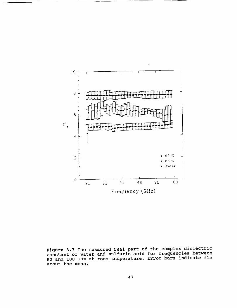
Similarly, the results of the measurements of the complex
dielectric constant at 90.0-100.0 GHz are shown in Figures 3.7
and 3.8. The error bars shown in these four figures represent
±Io variations in the calculated values of e_ I and e I/ZII
resulting from uncertainties in the thickness t of ±25.0 pm.
Hence these error bars do not include uncertainties due to
instrumental errors which are of the order of an additional
±3% of the reported mean values. (The variation in the size
of the error bars as function of frequency may be due to
errors in the convergence of the root finder program used to
determine the complex dielectric constant.)
3.4 Theoretical Characterization of the Dielectric Constant of
Liquid Sulfuric Acid (H2SO 4) at Millimeter-Wavelengths
In order to investigate the effects of cloud condensates
on the millimeter wave emission of Venus, a knowledge of the
complex dielectric constant of liquid sulfuric acid is
necessary over a wider frequency range. Although our
measurements were performed over a relatively narrow frequency
range (i.e., 30-40 and 90-100 GHz), a theoretical
characterization of the dielectric constant at other
wavelengths can be performed. Brand et al. (1953) measured the
46
10 i T T f I
J6
r
k
o i
-__...._,_.._.,._._..; .-_'
• 99%
• 85%
• Water
i I _ l , l
93 92 94 96 98 100
Frequency (GHz)
Figure 3.7 The measured real part of the complex dielectric
constant of water and sulfuric acid for frequencies between
90 and I00 GHz at room temperature. Error bars indicate ±la
about the mean.
47

r
14
12
I0
I I i I I
• Water
• 85_
• 99%
93 92 94 96 98 100
Frequency (GHz)
Figure 3.8 The measured imaginary part of the complexdielectric constant of water and sulfuric acid for
frequencies between 90 and 100 GHz at room temperature.Error bars indicate ±la about the mean.
48

dielectric constant of liquid sulfuric acid with
concentrations ranging between 96 and I00 % at microwave
frequencies. A best fit expression for their data was also
developed which is consistent with a model of the liquid
having multiple relaxation times. As a result, we have
developed a best fit model for our measured data based on a
semi-empirical equation developed by Cole and Cole (1941);
ezs- ez-¢_ = er. + (3.8)
I • II
where Er (er= £ r-JE r) is the complex dielectric constant, E_
is the real part of the dielectric constant at w-w, ers is the
real part of e r at d.c., T is the relaxation time (this
relaxation time is defined as the time it takes the induced
polarization to fall to i/e of its maximum value after the
removal of a constant applied electric field), and _ is a
constant between 0 and i. Equation (3.8) can be rewritten as
per King and Smith (1981) so that,
i l+wzZ-_sin(a_) _e_ = e_.+ (_s-e_.) (3.9)
1+2 (W_)z-_ sin (_) + (w_) 2(z-,)
and,
49

(_)1"cos(a 2)//e_ = (e_-e_.) 13.3.0)
1+2 (WT) I-. sin (e -_ ) + (w_) 2(i-.)2
In order to employ the above two equations to model our
measured data, the values of ers, _, 7 and _ must first be
determined. For the case of ers' its value is determined based
on the static dielectric constant of water and i00 % sulfuric
acid and the mole fraction of the concentration of interest.
That is,
m_2o + ers mH2s°4ers = ers.2° m T i00_.2so4inT
(3.11)
where er_ ° and er_so ' are the static dielectric constants of
H20 and 100% H2SO 4 and mx2o/m r and mH2so,/m r are the mole
fractions of H20 and H2SO 4 respectively. For the 85% (by
weight) liquid sulfuric acid used in our measurements, a value
of 87.5 is obtained for ers (Ers=80"4 for water and Ers=95.0 for
sulfuric acid, see Brand et al., 1953). The other three
parameters are determined by best-fitting the measured data
with equations (3.9) and (3.10). As a result, our expression
for the complex dielectric constant of 85% liquid sulfuric
acid is given by,
5O

er=3.3 + (87.5-3.3) (3.12)l+(jw(l.7xlO-11)(1-.o9)
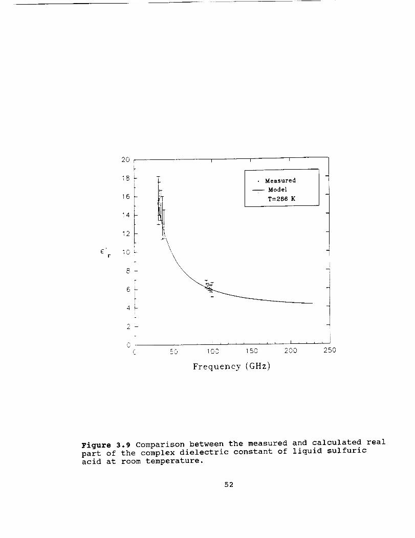
A comparison between our measured data and the
theoretically determined complex dielectric constant of liquid
sulfuric acid are shown in Figures 3.9 and 3.10. In Figure
!
3.9, c r is plotted against frequency while Figure 3.10
i!
represents e r versus frequency for 85% liquid sulfuric acid.
A closer examination of the two plots reveals that our data
agrees well with the values obtained from the developed model.
As a result, this new model will allow us to determine the
expected dielectric constant of liquid sulfuric acid at
frequencies other than the ones reported in this work. This
new formalism will be later incorporated into a radiative
transfer model to investigate the effects of liquid H2SO 4 on
the millimeter-wave emission of Venus.
51
2O I I I
6r
18
16
14
12
10, 1,,.,-
i'-
8,-
6"
\
Measured
-- Model
T=286 K
i
_: ,llJI,JILilllLh
C 50 100 150 200 250
Frequency (GHz)
Figure 3.9 Comparison between the measured and calculated real
part of the complex dielectric constant of liquid sulfuric
acid at room temperature.
52

E fl
r
25
2O
15
ii
10i
I
I
5 _!IL
0
i I I I
• Measured
-- ModelT=296 K
, , 1 , I L 1 _ L J
5'5 IO0 150 200 250
Frequency (GHz)
Figure 3.10 Comparison between the measured and calculated
imaginary part of the complex dielectric constant of liquidsulfuric acid at room temperature.
53

CHAPTER 4
VAPOR PRESSURE OF GASEOUS SULFURIC ACID (H2SO 4)
4.1 Introduction and Motivation
The laboratory measurement of the partial pressure of
gaseous sulfuric acid in equilibrium with liquid H2SO 4 is of
great importance in modeling the abundance of gaseous sulfuric
acid which is found in the middle atmosphere of Venus. First,
the laboratory measurement of the vapor pressure of H2SO 4
provides data needed for more accurate calibration of the
microwave opacity measurements of gaseous H2SO 4 made by Steffes
(1985). As a result, the calibrated opacity can then be used
to infer the expected abundance of gaseous sulfuric acid from
measurements of microwave opacity in the atmosphere of Venus.
In addition, the measurement of the partial pressure of
gaseous H2SO 4 is used to determine the saturation abundance of
gaseous sulfuric acid thus providing an upper limit for the
abundance of gaseous sulfuric acid in the atmosphere of Venus.
54

In the past, several researchers have attempted to
determine the partial pressure of gaseous sulfuric acid but
their results have not been consistent. For example, Esposito
(1983) used the theoretically-derived vapor pressure model of
Gmitro and Vermeulen (1964) for determining saturation
abundances of gaseous H2SO4, SO3, and H20 (the vapors which
accompany liquid sulfuric acid) in the Venus atmosphere.
However, because laboratory measurements by Ayers et al.
(1980) showed that the Gmitro and Vermeulen model
overestimated the partial pressures of these constituents by
a factor of about i0, Esposito simply scaled the Gmitro and
Vermeulen results by that factor for his model. While
laboratory data from Ayers et al. (1980) and Steffes (1985)
showed that the vapor pressures of gases accompanying liquid
sulfuric acid were indeed much lower than the Gmitro and
Vermeulen model, neither was able to directly measure the
partial pressure of the individual gaseous constituents. The
Ayers et al. experiment measured the acidity of the vapor
above 98% concentration of liquid sulfuric acid. However, the
relative proportion of this acidity which was due to gaseous
H2SO 4 (as opposed to that due to SO3) was calculated from the
Gmitro and Vermeulen model and was not directly measured.
Steffes (1985) measured volumes of liquid sulfuric acid
solutions which vaporized to equilibrate an evacuated chamber
in order to infer the vapor pressures of the accompanying
55

gases. However, he too used the theoretical results from
Gmitro and Vermeulen in determining the relative proportion of
gaseous HzSO4 and SO3. Consequently, Steffes (1985,1986)
estimated that about 47% of the gaseous H2SO 4 that vaporized
from a liquid sulfuric acid reservoir at 575 K dissociated to
form gaseous SO 3 and H20. Although this estimate resulted in
adequate results for an upper limit on gaseous sulfuric acid
vapor pressure, a direct measurement of the dissociation
factor (and hence the partial pressure of gaseous H2S04) is
necessary in order to unambiguously determine the abundances
of these gases and thus to infer their microwave properties.
An apparatus capable of measuring the partial pressure of
gaseous H2SO 4 for temperatures between 480 and 610 K has been
developed. Using this apparatus, we have been able to measure
the partial pressure of gaseous sulfuric acid for two liquid
concentrations (99% and 95.9% by weight). From the measured
pressure we have been able to develop a new best-fit
expression for the partial pressure of gaseous H2SO 4 as a
function of the temperature between 480 and 610 K. In
addition, the resulting measurements have enabled us to
compute the dissociation factor of gaseous H2SO 4 (i.e. the
percentage of gaseous H2SO 4 that dissociated to form gaseous
SO 3 and H20 ) along with a new expression for the equilibrium
constant, Kp. This new value of the equilibrium constant is
used with the results from Ayers et al. (1980) to determine
56

the partial pressure of H2SO4 for temperatures between 330 to
480 K (see appendix A).
The result of our measurements are used to infer the
saturation abundance of gaseous sulfuric acid in the
atmosphere of Venus. In addition, our results are applied to
previous laboratory results (Steffes, 1985) so as to obtain a
corrected expression for the microwave absorptivity
(normalized by the number mixing ratio) of gaseous H2SO 4 in a
CO 2 atmosphere at 2.24 GHz. The results of the corrected
microwave absorptivity in addition to the measured partial
pressure of sulfuric acid are used by Jenkins and Steffes
(1991) to determine the abundance of gaseous H2SO 4 in the
middle atmosphere of Venus.
A detailed description of the laboratory apparatus used
in the measurement of the partial pressure of sulfuric acid
and the measurement technique used are described in Appendix
A.
4.2 Application of the Measured Vapor Pressure of HzSO 4 to the
Atmosphere of Venus
A direct application of the measured partial pressure of
gaseous H2SO 4 (see Appendix A) is the correction of previous
laboratory measurements of the microwave absorptivity
(normalized by the mixing ratio) of gaseous sulfuric acid in
a CO 2 atmosphere at 2.2 GHz. The original data was reported by
57

250
2O0
150
100
f50
I 1 I I 1 I
Corrected
..... or__v 584 k
• 575
_S
0 , ,I I I I I I
0 1 2 3 _ 5 6 7
Press_e (acre)
Figure 4.1 Corrected measurements of the microwave
absorptivity of gaseous sulfuric acid at 2.24 GHz. Solid
line represents a best-fit multiplicative expression for the
absorptivity while the dashed line is the original
expression (Steffes, 1985).
58

Steffes (1985) in which he used the partial pressure resulting
from an assumed 47% dissociation factor when developing an
expression for the microwave opacity of gaseous sulfuric acid.
(His measurements were conducted at 575 and 564 K which are
well within our temperature range). As a consequence of our
direct measurements of the partial pressure of gaseous
sulfuric acid, the absorptivity measured by Steffes (1985) has
been readjusted to account for the variation of the
dissociation factor with temperature. The resulting plot of
the corrected absorptivity is shown in Figure 4.1 where the
solid line represents a best-fit multiplicative expression for
the absorptivity given as,
al 3 (dB km-l) _ 9.25xi09 q ( p ),s8 ( T )-3 (4.1)
where q is the volume mixing ratio of gaseous sulfuric acid,
P is the pressure in atm, and T is the temperature in Kelvins.
The error bars shown in Figure 4.1 represent ± la errors in
the absorptivity measurements but do not include uncertainties
in the mixing ratio.
Another important application of our results is shown in
Figure 4.2. In this figure, the dashed line represents the
saturation abundance of gaseous sulfuric acid based on our
measurements of the partial pressure of H2SO 4 and the pressure-
temperature profile of Venus reported by Seiff et al. (1980).
In addition, the solid line represents the abundance of
59

65
6_
55D
UJ
C
.de
2801
Saturation Vapor Pressure
I I I
e _e 2e 3_
t.42£04 RBUND_qNCE . P P f'.'l
4e
Figure 4.2 An abundance profile for gaseous sulfuric acid in
the atmosphere of Venus after Jenkins and Steffes (1991).
The dashed line represents saturation abundance of gaseous
HzSO 4 in the atmosphere of Venus.
60

gaseous H2SO4 in the Venus atmosphere inferred from a 13 cm
absorptivity profile obtained from the Pioneer-Venus radio
occultation studies of Jenkins and Steffes (1991), using our
corrected expression for the 13 cm absorptivity of sulfuric
acid (equation 4.1).
In short, our results have been used to correct
previously reported measurements of the microwave absorption
of gaseous H2SO 4. This provides a more accurate result for the
microwave absorption of sulfuric acid within the atmosphere of
Venus. The resulting abundance profiles of gaseous sulfuric
acid can then be used to study the effects of this gas on the
chemistry and the millimeter-wave emission of Venus.
61

CHAPTER 5
MEASUREMENT OF THE OPACITY OF GASEOUS SULFURIC ACID (H2SO 4)
AT W-BAND (94.1 GHZ)
5.1 Motivation
As discussed in the previous chapters, a complete
understanding of the millimeter-wavelength emission from Venus
requires an accurate determination of the opacities of the
major absorbers in the Venus atmosphere. Recent observations
of the millimeter-wave emission from Venus at 112 GHz (2.6 m m)
have shown significant variations in the continuum flux
emission (de Pater et al., 1991) which may be attributed to
the variability in the abundances of absorbing constituents in
the Venus atmosphere. Such constituents include gaseous H2S04,
SO2, and liquid sulfuric acid (cloud condensates). Recently,
Fahd and Steffes (1991) have shown that the effects of liquid
H2SO 4 and gaseous SO 2 cannot completely account for this
measured variability in the millimeter-wave emission of Venus.
62

To fully understand potential sources of this variation, one
needs to study the effects of gaseous sulfuric acid on the
millimeter-wave emission of Venus.
Unfortunately, little (if any) laboratory work has been
performed to measure the opacity of gaseous H2SO 4 at
millimeter-wavelengths for Venus-like conditions. In addition,
the simple extrapolation of the microwave opacity of H2SO 4
measured by Steffes (1985,1986) to higher frequencies is not
straightforward and could lead to erroneous results.
To investigate the role of gaseous H2SO 4 in the atmosphere
of Venus, we have measured the opacity of gaseous H2SO 4 in a
CO 2 atmosphere at 550, 570, and 590 K from 1 to 2 atmospheres
total pressure at 94.1 GHz. This work represents the first
time that a measurement of the millimeter-wave opacity of a
H2SOJCO 2 gaseous mixture has been conducted for Venus-like
conditions. We have also developed a modeling formalism to
calculate the expected opacity of this gaseous mixture at
other frequencies based on our measured results and the
results reported by Steffes (1985,1986). Comparisons between
the measured and the theoretically derived opacities of
H2S04/CO 2 mixture are also presented.
63

5.2 Laboratory Configuration
The experimental system used to measure the millimeter-
wave opacity of gaseous H2SO 4 in a CO 2 atmosphere consists of
two major subsystems: The planetary atmospheric simulator and
the millimeter-wave subsystem as diagrammed in Figure 5.1.
The planetary atmospheric simulator subsystem consists of
a glass cell (which contains the gaseous mixture), two
pressure gauges, a thermocouple display unit, a CO 2 tank and
an oil diffusion vacuum pump. In this subsystem, the glass
cell (length=27") is placed into a temperature controlled oven
with a maximum temperature of 600 K. The temperature of the
oven is electronically controlled, with a temperature
variation of less than ± 5 K. A calibrated thermocouple unit
is inserted into the glass cell in order to display the
system's temperature. Liquid sulfuric acid is deposited into
a custom made flask prior to the start of the measurements.
The pressure and vacuum status of the planetary atmospheric
subsystem are monitored via two gauges. Gauge P (0-80 psig)
with a display resolution of 1 psig and an accuracy of ± 3
psig is used to measure the internal pressure of the glass
cell resulting from the introduction of the H2S04/CO 2 gaseous
mixture into the system. Gauge V is a thermocouple vacuum
gauge that is able to measure pressures between 0-800 Torr
with 1 Torr display resolution and an accuracy of 1% of full
scale. It is used to monitor the vacuum status of the glass
64

_0
I i _
c_
oj
\ /
Figure 5.1 Block diagram of the atmospheric simulator as
configured for measurements of the millimeter-wave
absorption of gaseous H2SO 4 under Venus atmosphericconditions at 94.1 GHz.
65

cell. Two Pyrex-66 glass windows are installed on the two
sides of the oven to allow the propagation of the
electromagnetic energy. A network of 3/8" stainless-steel
tubing and valves connect the components of the planetary
atmospheric subsystem so that each component may be isolated
from the system as necessary. An oil diffusion pump is used to
evacuate the glass cell prior to the introduction of the
gaseous mixture.
The millimeter-wave subsystem (also shown in Figure 5.1)
consists of a Siemens backward wave oscillator (BWO) powered
by a MicroNow power supply. The BWOis electrically isolated
from the waveguide apparatus by use of a polyester sheet and
nylon screws on the waveguide flange of the BWO. (this is
necessary to insure phase locking stability). Enroute to the
glass cell, the signal is first sampled by a 10dB directional
coupler. The sampled signal passes into a harmonic mixer as
part of the phase locking system. The majority of the signal
goes on through an isolator, which prevents reflections to the
BWO, and is then electronically chopped by a ferrite modulator
before entering the cell. The received power is detected by a
schottky barrier point contact diode detector at 94 GHz. Power
changes are measured as voltage changes at the detector. In
order to give the detector the most linear response, the diode
is biased with a current of I0 mA. The detector's output is
measured with a lock-in amplifier where the modulation
66

reference comes from a function generator which drives the
ferrite switch. The modulation frequency is I00 Hz. The output
of the lock-in amplifier is fed into a digital voltmeter.
Phase locking stabilizes the frequency output of the BWO.
The -10dB port of the directional coupler feeds the BWO output
into the harmonic mixer where it is heterodyned with the local
oscillator (LO). A synthesized signal generator (2-18 GHz)
serves as the LO and as the reference signal for the phase-
locked loop. The intermediate frequency (IF) from the mixer is
fed into the phase detector. The phase-locked loop functions
only when the LO harmonic is below the BWO frequency, i.e.,
setting the LO to 9.368 GHz gives 9.368 GHz x I0 = 93.680 GHz
+ 420 MHz IF = 94.1 GHz. An IF monitor output on the phase
detector allows viewing the locked waveform with a spectrum
analyzer.
In order to minimize the effect of any reflections from
the cell wall, the radius of the cell must be chosen greater
than the radius of the first Fresnel zone (the Fresnel zone is
defined as that volume surrounding a ray path through which
another ray can travel and arrive at the receiver having
travelled no more than 1/2 wavelength farther than the primary
ray; Bullington, 1957). Thus, it follows that
67

R c > , (5. I)
where R c is the radius of the cell, A is the wavelength (in
this case 3 mm), and r is the separation distance between the
two horns (i m). Using the above equation, a minimum cell
radius of 1.52" is required. A glass cell with a radius of
2.5" is used in the experimental setup.
5.2.1 Measurement Procedure
The measurement of the millimeter-wave opacity of gaseous
H2SO_/CO 2 can be summarized as follows: The oven is first
heated to the desired temperature. Once the desired
temperature is reached, the glass cell is evacuated. By using
gauge V as a vacuum monitor, we are able to check the status
of the glass cell in order to insure that no major leaks are
present. Although the chamber is not leak proof, we are able
to maintain a leak rate within the system of less than 1
Torr/hour. The variable attenuator is then set to a
predetermined attenuation and the resulting detector voltage
is recorded. (The millimeter-wave subsystem is usually turned
on for a period of ten hours prior to the beginning of the
experiment. This extended time period allows the BWO to warm
up and become more stable.) Next, the valve connecting the
H2SO 4 flask and the glass cell is opened allowing the sulfuric
acid vapor to equilibrate with the evacuated glass cell. Once
68

equilibrium is reached, the flask's valve is closed and a
visual check is made to verify that the remaining liquid acid
is clear. Gaseous CO2 is then introduced in the system at a
slow rate so as not to cause any condensation. When the total
internal pressure (measured by gauge P) reaches 2 atm, the CO2
tank is shut off and the two gases are allowed to mix for a
specified time period. The attenuation on the variable
attenuator is then decreased until the output voltage is equal
to the detector voltage of the evacuated glass cell. The
opacity of the gaseous mixture can then be inferred from the
change in the calibrated attenuator setting. The total
internal pressure is then reduced to 1 atm and the measurement
process is repeated. This approach has the advantage that the
same gas mixture is used for the measurement at various
pressures (at each temperature point). Thus, even though some
uncertainties may exist due to the mixing ratio of the initial
mixture, the mixing ratios at subsequent pressures will be the
same, and the uncertainties for any pressure dependence will
only be due to the accuracy limits of the absorptivity
measurements and not to uncertainties in the mixing ratio.
5.3 Experimental Uncertainties
In general, the main source of experimental uncertainties
in the transmission measurements are the fluctuation in the
output power of the source. However, our system is phase
69

locked so as to minimize frequency and output power
deviations. Frequency stabilization due to the phase locking
system is approximately ± 20 KHz and power variation is less
than ± .02 dB. In order to incorporate the effect of frequency
and power fluctuation in our error bars, two measurements are
taken for each data point and statistics are developed to
compute the 1 a variation in the measured absorptivity (the
number of data points collected was limited due to the
availability of some of the equipment).
Additional instrumental uncertainties include
uncertainties in the measured pressure and temperature. In the
case of pressure measurements, the accuracy was limited by the
quality of the two pressure gauges used. The 0-800 Torr gauge
has an accuracy of 1% of the full scale while the 0-80 psig
gauge has an accuracy of ± 3 psig. The temperature accuracy of
the thermocouple used was ± 5 K (temperature uncertainty is
shown as horizontal error bars in Figure 5.2). The accuracy of
the variable attenuator is also incorporated in our total
uncertainties. The uncertainties due to the mixing ratio have
been determined for the three temperatures used in our
measurements. Using the expression developed by Spilker (1990)
for mixing ratio accuracy, mixing ratios of 1.25% ± 0.13%
,0.87% ± 0.087% and 0.59% ± 0.06% are obtained at 590, 570,
and 550 K respectively (in this calculation the partial
pressure of H2SO4 is obtained using equation (5.2)). These
70

70OO
6000
'_ 5000
0,Iml
4000
3000
oo_,_
J_
2000
¢(D
1000
--VVW model
• I Atm
• 2 Atm
: I
I
. a :w
i I i I I i I I ; | ' i . i _ i | J i
520 540 560 580 600
Temperature (K)
Figure 5.2 Laboratory measurements of the normalized
absorptivity (dB/km) of gaseous HzSO 4 in a CO 2 Atmosphere at94.1 GHz. Solid curves are the theoretically calculated
absorption from the VVW formalism.
71

mixing ratios uncertainties are also included in the vertical
error bars shown in Figure 5.2.
Additional experimental uncertainties include the
detector's noise which was characterized from variations in
the measured output voltage. The resulting total uncertainties
due to noise and instrumental uncertainties are shown in
Figure 5.2 as ±i a variations about the mean. Finally, an
estimate reflecting the effects of multiple reflections from
the glass plates on the measured absorption has been added to
the error bars of Figure 5.2.
5.4 Experimental Results and Theoretical Characterization of
H2SO4Absorption
Measurement of the opacity of gaseous H2SO 4 in a CO 2
atmosphere has been performed at 94.1 GHz and at temperature
of 550 K, 570 K, and 590 K. These temperatures were chosen so
as to allow enough H2SO 4 vapor in the glass cell. The
experiment was conducted at total pressures of 2 and 1 atm for
each temperature. For a specific pressure and temperature, the
expected vapor pressure of H2SO 4 can be computed by (see
appendix A),
inp=6.65 -610----_0 (5.2)T
where p is the sulfuric acid vapor pressure (atm) and T is the
temperature in K. Using the above expression, a mixing ratio
72
of 1.23%, .87% and .59% occurs respectively at 590, 570 and
550 K.
The measured absorption (dB/km) of H2SO4/CO2 at 94.1 GHz
is shown in Figure 5.2 where it is plotted as a function of
temperature for 2 and 1 atm. (note that the reported
absorptions are normalized to their respective mixing ratios).
Using the measured data, a best fit multiplicative expressions
has been developed to predict the absorption of H2S04/CO 2 at
94.1 GHz,
a =2xlO11p'98qT -2"9 dB/km (5.3)
where q is the H2SO 4 number mixing ratio, P is the total
pressure in atmospheres, and T is the temperature in Kelvins
(in the above equation, the pressure and temperature exponents
are fitted to the measured data).
Although the developed expression is valid for the
conditions at which the measurements were performed (i.e. 94.1
GHz), care must be taken when projecting the absorption of
H2SO 4 at frequencies far from 94.1 GHz. To accurately determine
the expected absorptivity at other frequencies, we have used
the Van Vleck-Weisskopf (VVW) formalism to calculate the
opacity of the H2SOJCO 2 gaseous mixture. In this formalism,
the absorptivity due to a single resonant line, at frequency
f, can be computed as per Townes and Schawlow (1955),
73

a=a_f2 v_2 6v2[((vo_f)2+6v2)-1+((Vo+f)2+6v2)-1] (5.4)
where f is the frequency in GHz, v o is the resonant line
frequency, and 6v is the line width. In our VVW model, we
totaled the contribution from 2359 resonant lines reported by
Pickett et al. (private communication, 1991). These lines
cover the frequency between 1.5 and 450 GHz. A graphical
representation of the resonant lines and their respective line
intensities, Iab, are shown in Figure 5.3 along with an
expanded view of the lines between 1.5 and 40 GHz.
In order to fully implement the VVW formalism, an
appropriate broadening parameter, 6v, must be determined.
Previously, Janssen and Poynter (private communication, 1987)
used a value of 3 MHz/Torr in their model (their model used a
different set of resonant lines) but their results were
inconsistent with the measured microwave absorptivity of
Steffes (1985,1986). In addition, no measurements of the
broadening parameter of H2SO _ by CO 2 have been reported. To
solve this problem, we adjusted the broadening parameter in
the VVW formalism so that the calculated opacity matches the
measured absorptivity at 94.1 GHz and the microwave absorption
at 2.24 GHz and 8.42 GHz reported by Steffes (1985). As a
result, a broadening parameter of 1.55 MHz/Torr was found to
fit the above data and seem to provide close agreement between
the measured and calculated values of the absorptivity of H2SO 4
74
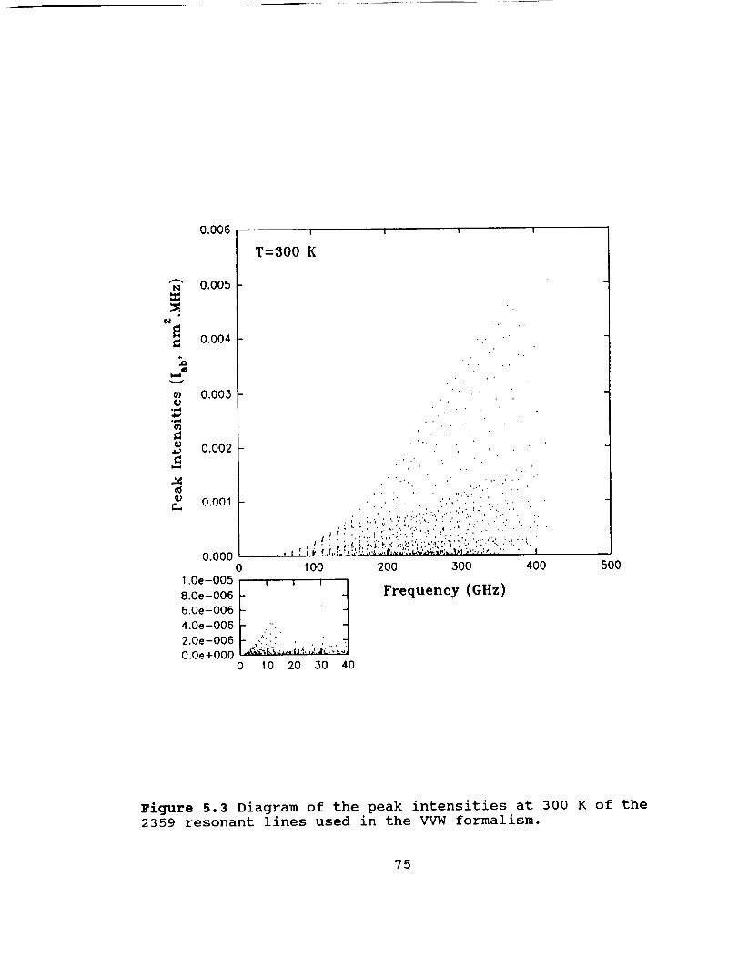
[,,1==
0,1
,e
v
%)op,,4
o=,-I
c
13.,
0,006
0.005
0.004
0.003
0.002
0.001
T=300 K
. ..
0.0000 100
1.0e-O05 , , , j
J6.0e-006
4.0e-006
2.0e -006 _j _,i,_,.:_,:::.,.O.Oe+ 000 ....
0 10 2O 3O 40
., , ,. . . ., ,... , .
',. , . ' ,.. '..
' ". ;'" _ "'i"'"' ......... .."" "" '; , , , , '..;,. '- :,• . • ,
2O0 300 40O
Frequency (GHz)
5OO
Figure 5.3 Diagram of the peak intensities at 300 K of the2359 resonant lines used in the VVW formalism.
?5

in a CO 2 atmosphere.
A comparison between the calculated and measured
opacities of H2SO4/CO2 are shown in Figures 5.2, 5.4, and 5.5
where the discrete data points in Figures 5.4 and 5.5 are
obtained from Steffes (1985). In Figure 5.4, the calculated
absorption of H2SO4/CO2 mixture at 2.24 GHz and temperatures of
564 and 575 K are compared with the previously published work.
Similarly, Figure 5.5 shows the results at 8.42 GHz and
temperatures of 550 and 520 K. A careful examination of these
results indicates that the calculated opacities of H2SO 4 using
the VVW formalism with a broadening parameter of 1.55 MHz/Torr
agree well with the measured microwave and millimeter-wave
opacities of the gaseous mixture. This finding is quite
important since it demonstrates for the first time that the
VVW formalism can be used to accurately predict the opacity of
H2SO4/CO2 gas mixture over a wide frequency range. As a result,
we can use the developed model to predict the opacity of H2SO 4
at other specified conditions and in particular, we can employ
the VVW formalism in our radiative transfer model to study the
effects of this gaseous mixture on the emission from Venus.
76

I
180
160
140"0
_t _2o
•- 100.4"_
o 80
o60
I,.,0In
"_ 40
2O
I I ! i
f-2.24 GHz..... VV_ at 564 K
_VVW at 575 K• 564 K0 575 K
I I I i0 I I0 I 2 3 4 5 6
Pressure (arm)
Figure 5.4 Comparison between the measured absorption
(normalized by mixing ratio) of H2SO 4 (Steffes, 1985,1986)and the calculated absorption from the VVW formalism at 2.24
GHz.
77

I
E
o_
%==
2200
2OOO
1800
1600
1400
1200
1000
8000
r,.)
6000
e_ 4000
•_ 200
0
( I
F--8.42 GHz......V'_ at 530 K_YYW at 520 K
• 520 K0 530 K
j I I !
1 2 3 4
L 1
5 6 7
Pressure (atrn)
Figure 5.5 Comparison between the measured absorption
(normalized by mixing ratio) of H2SO 4 (Steffes, 1985,1986)and the calculated absorption from the VVW formalism at 8.42
GHz.
78

CHAPTER 6
MODELING OF THE ATMOSPHERE OF VENUS
6.1 Development of the Radiative Transfer Model
In the previous chapters, detailed descriptions regarding
laboratory measurements of the millimeter-wave opacity of
constituents of the Venus atmosphere were presented. In order
to study the effect of these constituents (and other possible
absorbers) on the millimeter-wavelength emission from Venus,
a radiative transfer model has been developed. This model
incorporates the results of our measurements in addition to
other data that is pertinent to the atmosphere of Venus.
In the classic theory of radiative transfer, the radiated
energy of a black body (also known as brightness) in units of
Watts per square meter per hertz per steradian (Wm-2Hz-ISr'1),
is related to its physical temperature through the Planck
function given as (Liou, 1980),
79

C_
OII
TT TYTyy
\
Figure 6.1 Sketch of the geometry of the planet Venus.
8O

2by 3B v (T) -
2 hv
where v is the frequency, c is the speed of light, h is
Planck's constant (6.63xi0 "34 J s) and k is Boltzman's constant
(1.38xi0 -23 J/k). The geometry of the planet Venus used in the
radiative transfer model is shown in Figure 6.1 where the
zenith angle at a given point ,Y, is defined as the angle
between the normal to the surface and an observer's line of
sight to that point. The quantity _ is defined as the cosine
of the zenith angle y. In general, the total brightness
emitted at the top of the atmosphere (Z=0) along a path in the
direction of _ is given as (Liou, 1980);
-[ Zsuzf'ce ¢¢_, ( Z/) dz----/
S v(T,_) =B v(T s) e _o
z_._._ -/o* =. (z I) dzl ( 6 • 2 )+f0 BY (T(z) ) e -_ ¢v (z) d__zz
where z is the depth as measured from the top of the
atmosphere, and _v(z) is the total absorption coefficient of
all absorbing constituents at depth z and frequency v. The
total brightness can also be written as function of the
weighing function Wv(z,v ) which describes the locations within
the atmosphere which contribute most to the total brightness,
81

:fzsu,t.co;_ (T(z) ) Wv(z,v) dzBY (T' _) J0 --" -_
(6.3)
Another expression which is usually employed in radiative
transfer modeling is the vertical optical depth, r, defined
as,
_0 Zz,(Z) = av(Z I) dZ / . (6.4)
Upon substituting equation (6.4) into (6.2), we obtain an
alternate form of the radiative transfer equation,
T_ __
Bv(T,_ ) =Bv(Ts) e--_+fo*Bv(T(zl) ) e _ dz/ (6.5)
where r I is the optical depth at the planet's surface.
Radio emission from planets is usually given as a
brightness temperature, T B, which is the temperature at which
a blackbody would radiate an intensity of electromagnetic
radiation identical to that of the planet at a specific
frequency. The brightness is related to the brightness
temperature via Planck's function;
82

hv
( 2hv 3 ) (6.6)k in _ Bc 2 +I
6.2 Disk Average Brightness
The disk average brightness of a planet, Bv(TD), can be
obtained by integrating equation (6.5) over all angles of
incidence thus,
LBv(TD) =2 Bv(T,_) _d _ . (6.7)
Upon substituting equation 6.5 into 6.7 we obtain,
Bv(_)=2 Bv(gs) e _d_+2 By [T(z/)]e_,,/_dz/d _ (6 8)
where the first term is the brightness of the surface observed
at the top of the atmosphere reduced by the absorption of the
intervening layers by a factor e -_I/_. The second term of
equation (6.8) corresponds to the brightness emanating from
within the atmosphere of Venus.
For a simple spherical planet, the integration may be
simplified to a single exponential integral (Goodman, 1969) so
that,
fo r_Bv(_)=2Bv(_)_(Tz)- 2 Bv(T(T/))dE3(_/) (6.9)
where,
83

En ( _ ) =_'--._ne-'Ydy (6.10)
and y=l/_. In the developed model, the weighting function at
a particular frequency is computed via _(z)=T(z)dE3(r(z)) .
Numerical implementation of the radiative transfer model
has been achieved where the integral in equation (6.9) is
evaluated by dividing the atmosphere into discrete layers as
shown in Figure 6.1. The average pressure, temperature, and
altitude at each discrete layer (each layer has a thickness of
1 km.) are determined using the pressure-temperature profile
described by Seiff et al. (1980). The integration is evaluated
starting at the top of the atmosphere (Z=0) and is terminated
at the surface of the planet. The brightness at each layer is
evaluated in addition to the corresponding optical depth of
that particular layer. The contributions from each layer are
then added to yield the total brightness and hence the disk-
averaged brightness temperature of the planet.
6.3 Parameters of the Radiative Transfer Model
To fully implement a radiative transfer model, several
variables must be included in the model. Such variables
include the pressure-temperature profile of the atmosphere of
the planet, the expected opacities of the major atmospheric
84

constituents, and the distribution
constituents within the atmosphere.
of these absorbing
6.3.1 Pressure-Temperature Profile of Venus
Several pressure-temperature profiles of Venus have been
developed using data from entry probes released in the
atmosphere of Venus in the late seventies. Seiff et al. (1980)
developed such profiles using the collected data from the four
Pioneer-Venus entry probes. In our model, the profile obtained
from the sounder probe (released over the equator of Venus) is
employed. A plot of this pressure and temperature profile is
shown in Figure 6.2 as function of altitude. In addition, a
standard disk radius of 6120 km is used for Venus (the
standard disk radius includes the physical radius of the
planet in addition to the height of the atmosphere).
6.3.2 Gaseous CO 2 Absorption
Gaseous carbon dioxide (CO2) is considered to be the
major absorber in the atmosphere of Venus. The absorption from
CO 2 can be attributed to the collisions of CO 2 molecules in the
atmosphere of Venus. Ho et al. (1966), determined the
following expression for the absorptivity, u, of a mixture of
CO 2 and N 2 under high pressure;
85

100 _
8O
60 i", \
'\
40 - \
i
\
!
20-L
F
i
OLO
LL
i ......... Temperature--Pressure
800
J
700
600 ,-.
500
i
" 400 _
,300
I , L ,"-T-"--_, , I , , , 200.... 60 80Z O "" "-#
Altitude (KM)
Figure 6.2 Pressure-Temperature profile of the atmosphere of
Venus.
86

where p is the pressure in atmospheres, T is the temperature
in K, f is the frequency in GHz, and q is the number mixing
ratio. For the atmosphere of Venus, CO 2 composes about 96% of
the atmosphere while N 2 corresponds to about 3.0 % (Steffes,
1982). In the development of the radiative transfer model, the
above expression is used to compute the opacity of gaseous CO 2
in the atmosphere of Venus. A plot of the expected absorption
of CO 2 in the atmosphere of Venus is shown in Figure (6.3),
where the absorption (I/km) is plotted as a function of
altitude for 30, 50, 75, i00, and 125 GHz, based on the T-P
profile of Seiff et al., (1980).
6.3.3 SO2-CO2Absorption
As we demonstrated in Chapter 2, the results from the
measured opacity of gaseous SO 2 in a CO 2 atmosphere indicate
that the Van Vleck-Weisskopf formalism can be used to
determine the opacity of sulfur dioxide for Venus-like
conditions at wavelengths shortward of 1.5 cm. This key
finding differs from previous results of Steffes and Eshleman
(1981) and Janssen and Poynter (1981) which suggested that the
microwave opacity of SO 2 had an f2 dependence. As a result of
our finding, we have incorporated the VVW formalism in our
radiative transfer model to infer the expected opacity of
87

<
2O
i0
5
0
I 5 _ , _
-20
C02 absorption-- 30 GHz
--- 50 GHz
..... 75 GHz
......... 100 GHz
......... 125 GHz
• "° ,
0 20 4 0 6 O 8 0
Altitude (KM)
Figure 6.3 Expected absorption of gaseous CO 2 in theatmosphere of Venus based on the results of Seiff et al___.
(1980) and the results of Ho et al_ (1966).
88

O
05
C 3
L t "
L
L
i 1
S02-C02 Present30 GHz
--- 50 GHz
..... 75 GHz
......... 100 GHz
......... 125 GHz
-0.1- 20 0 _ _ 43 z,S 80
Altitude (Km)
Figure 6.4 Absorption profiles for gaseous SO 2 in a CO 2atmosphere according to the VVW formalism and the T-p
profile of Seiff et al____.(1980) (SO 2 abundance: 62 ppm).
89

gaseous SO 2 under Venus-like conditions. Typical absorption
profiles of gaseous SO 2 in a CO 2 atmosphere are shown in Figure
(6.4) where the absorption of gaseous sulfur dioxide (I/km) is
plotted versus altitude for a specific T-p profile of Venus at
30, 50, 75, i00, and 125 GHz, assuming an SO 2 abundance of 62
ppm.
6.3.4 Liquid Sulfuric Acid Condensates
As discussed in Chapter 3, liquid sulfuric acid is known
to exist in the form of clouds within the atmosphere of Venus
where the more dense lower cloud layer extends between
altitudes of 48 and 50 km, (Knollenberg and Hunten, 1980).
However, its effects on the millimeter-wave emission from
Venus are not fully understood. To fully understand its role
on the emission of Venus, its absorptivity must be determined
so as it can be employed in a radiative transfer model.
In general, when an electromagnetic wave propagates
through a cloud layer, it is scattered and absorbed by cloud
particles. For a plane wave with a wavelength l, incident upon
a spherical particle with radius a, the absorption cross-
section is given as,
Absorbed Power (W)Q_: (6.12)
Incident Power density (W/m 2)
and the scattering cross-section is given by,
9O

Qs = Scattered Power (W) (6.13)Incident Power density (W/m 2)
For a dielectric sphere with a complex relative permittivity
Er, the absorption and scattering cross-sections are
respectively (Ulaby, 1980),
12 _ (2n+l)(lanl 2+Ibnl 2) (6.14)Qa 2_ n-1
and,
12 _ (2n+l) Re (an+bn) (6.15)Qs 2_ n-1
where Re signifies "real part of", and a n and bn are the Mie
coefficients which are function of _r and a. For the case
where the droplet dimension is much smaller than l, the
absorption and scattering cross-sections are reduced to what
is referred to as the Rayleigh approximation where,
and,
212 x61kl2 (6.16)Qs - 3_
_2Qa - X 2 Im(-k) (6.17)
where Im signifies "the imaginary part of", and k is a complex
quantity related to the complex index of refraction _, by
91

and
/_2-I e-ik - - (6.18)
_2+2 ¢+2 '
2ha (6.19)X- l
Thus, if I_XI < .5, the absorption and scattering cross-sections
can be evaluated using the Rayleigh approximation while if
i_Xl >.5, the Mie coefficients must be used (Ulaby et al.
1980).
For a typical cloud layer, the volume extinction
coefficient (Ke) is the sum of the absorption and scattering
coefficients (Ulaby et al., 1980);
ac:oud=_[Qa<ri) +Qs(ri)] = K e = Ka+ G(6.20)
where N v is the number of particles per unit volume and r i is
the radius of the i th particle. K a and K s are the volume
scattering and volume absorption coefficients respectively
(i.e., the total scattering (absorbing) cross-section per unit
volume).
For the case of the Venus atmosphere, extensive studies
of the physical parameters of the cloud condensates have been
performed using data from several entry probes. Knollenberg
and Hunten (1980), determined conservative upper limits of 25
microns for droplet size and 50 mg/m 3 for cloud bulk density.
92

°m
E
_J
O O
o9 c_
i I
\\
\\
\
UOll_as s$o_3 UOl_Cl_osqv
C_ _
C .Q
O_
.C3
\\
\\\
t',,lT-
u_00
00÷
W0C_
c_
u_ _ w w u_0 C3 0 0 0(_ 0 0 0 0
\
\
,°
%
0
C_
0
00
0oO
00
0
\\I°
0 0
N o
0qD
T-
uol_3as sso_ 3 8ul._a_...le:_S
Figure 6.5 Comparison oZ the scatterlng and absorbing cross-
section of liquid sulfuric acid droplets with radius of 12.5
microns at room temperature (296 K).
93

Using this information and our results regarding the complex
dielectric constant of sulfuric acid (see Chapter 3), the
scattering and absorption cross-sections for such a condensate
have been computed. Plots of the computed cross-sections are
shown in Figure (6.5). An examination of the results indicates
that the absorption cross-section is many orders of magnitude
greater than the scattering cross-section for 25 micron
particles at the temperature and with composition
characteristic of the lower cloud deck of Venus. Since the
absorption cross-section is much greater than the scattering
cross-section, the volume extinction coefficient can be
approximated by (Battan, 1973),
246 Me 11_ clou_ = (dB/km) (6.21 )
where p is the density of the liquid sulfuric acid and M is
the bulk density of the cloud (bulk density= total mass
occupied by cloud particles per unit volume) in the same
units, I is the wavelengths in km and e r' and er" are the real
and imaginary parts (respectively) of the complex dielectric
constant of the liquid.
Using our model for the complex dielectric constant of
H2SO4, the expected opacity (I/km) of liquid sulfuric acid has
been computed using equation (6.21). The results of this
calculation are shown in Figure 6.6. In this figure, the real
94

U
4U'C
O
O_
oO
b
cOO O
(U'_ll I ) U°l_'enua_v
O CD _, CD
o c_ o o
I t I t I
O
O O
c.o_
_D
Li
0 0 0 0 0 0 0 0
uoiisd_jo _d "mI'le_I
0
oO0c_
o9oO
T-
cO
Figure 6.6 Expected absorption (i/km) and dielectric
properties of an 85 % (by weight) liquid sulfuric acid
solution with a bulk density of 50 mg/m 3 and a droplet
radius of 12.5 microns.
95

and imaginary parts of the complex dielectric constant of
sulfuric acid are also plotted in addition to the expected
absorption of H2SO 4 for a typical cloud layer in the atmosphere
of Venus. Results from equation (6.21) will be incorporated
into the radiative transfer model in order to investigate the
effects of sulfuric acid cloud condensates on the millimeter-
wave emission from Venus.
6.3.4.1 Scattering Effects of the Cloud Condensates
Although the scattering cross-section of a single H2SO _
droplet is much smaller than its absorbing cross-section, the
effect of the bulk density of the condensates must be
evaluated when computing the back-scattering from a cloud
layer. This backscattering effect can cause a cooler
brightness temperature due to reflection of the cold sky. To
investigate the significance of this phenomenon on the
emission of Venus, we have computed the expected transmission
and reflection coefficients for a typical cloud layer in the
atmosphere of Venus.
For a cloud made up of discrete homogeneous layers and
assuming that radiation is scattered in only the forward and
backward directions, the transmission and reflection
96

coefficients of a
(Gasiewski, 1990),
layer with thickness dz are given as
wtec = (6 •2 2 )
1 +___2 coth (ecdz)
and
_[___2 csch (_cdz)tec = (6.23)
l +%/l-w2 coth (acdZ)
respectively, where _c is the total power attenuation from the
cloud which in the case of Venus includes the absorption from
gaseous CO 2 and liquid sulfuric acid. The quantity _c can be
written as (Gasiewski, 1990),
ac = _k2a +2kaksb(6.24)
where ksb is the back-scattering coefficient. The quantity w
is referred to as back-scattering albedo given as,
-- ksbw - (6.25)
k_+ ksb
The back-scattering coefficient, ksb, can be determined from
the scattering-coefficient, k s, and the phase fraction
asymmetry, g, of the clouds as,
97

For a spherical droplet, the asymmetry phase function is equal
to zero. In this case:
k - kssb- -_- (6.27)
which indicates that the scattered wave is equally divided in
a forward and a backward direction.
Since the cloud is made up of several discrete layers, a
composite transmission and reflection coefficient can be
computed based on the transmission and absorption coefficients
by (Paltridge and Platt,of two adjacent layers (a and b)
1976) where,
2tar a
rab = ra+1 -tar b
(6.2e)
and,
tab - ta tb . (6 •29 )l-rat b
Using the above two equations, we have determined the
composite reflection and transmission coefficient for the H2SO 4
cloud layer of Venus. A mass density of 50 mg/m 3 with droplet
diameters of 25 microns are used in our computation. The
results reported in Chapter 3 concerning the complex
dielectric constant of H2SO 4 are also used in the calculation.
98

U
U
0 0 0 00 0 0 0
0 0 0 0
\
.8 8
._ .g_E _
I--IIII
!
I
II
/
I
t
I
I
It
1
I
I
I
/
I
Iif I
o
•po:) u0p,3aUal:lcO _ 'q" 040 0 0 00 0 0 0
0 0 0 0 00 0 0 0 0o o o. o. o0 0 0 0 0
I I iI I II
It
\ I
"\ I
I
I
/I
t'\
/ \
/ \\!
t \,t \
I \, \
I
I
t '\
I \I ,,
i \
/I/
/
/ \t
O
O
O
OO
O
OCD
OO,r-
O
OCD
O
O
i I I I I I I I _
0 0 0 0 0 0 o o
•j._o_) UOlSl"'sueJJ.
Figure 6.7 Transmission and reflection coefficient for the
H2SO 4 cloud layer in the atmosphere of Venus.
99

A graphical representation of the results is shown in Figure
6.7 where the transmission and reflection coefficient are
plotted as a function of frequency for a cloud layer with
thickness of 2 km. An examination of the results indicate that
the cloud layer is mostly transmissive and the reflection
coefficient is very small. Thus, back-scattering does not have
a major role in the observed variations in the millimeter-wave
emission from Venus.
6.3.5 Gaseous H2SO4-CO2Absorption
As reported in Chapter 5, the VVW formalism provides an
accurate means for computing the expected absorptivity from
gaseous sulfuric acid in a CO 2 atmosphere at microwave and
millimeter-wavelengths. This important finding allows us to
integrate the opacity of H2SO_/CO 2 gaseous mixture in our
radiative transfer model so as to investigate its effect on
the millimeter wavelength emission from Venus.
Using the VVW formalism, we have computed several
absorption profiles of H2SOJCO 2 gaseous mixture using the
pressure-temperature profile of Seiff et al. (1980) and a
gaseous abundance of 25 ppm. The absorption profiles are shown
in Figure 6.8 for frequencies of 30, 50, 75, 100, 102.5, 113,
125, and 143 GHz. In addition, we have plotted the
absorptivity of this gaseous mixture versus frequency for a
single pressure and temperature point which is relevant to the
i00

atmosphere of Venus (in this case, the pressure and
temperature are for 42 Km altitude). An examination of this
profile, shown in Figure 6.9, reveals that the absorption
appears to go through several local peaks . This result is
quite interesting since it demonstrates for the first time
that the expected absorptivity is not a monotonically
increasing function. This phenomenon well explains the results
of Figure 6.8 where the absorption at 102 GHz is larger than
the absorption at 125 GHz for altitudes above 42 km.
6.3.6 HzO Vapor
Although water vapor is known to exist in the atmosphere
of Venus, discrepancies regarding its abundance are still
unresolved. Estimates using the Pioneer-Venus gas
chromatography (PVGC) experiment (Oyama, 1979) place the HzO
concentration on the order of several thousand ppm. Other
measurements of H20 vapor range from 20 to 200 ppm. Recently,
Lewis and Grinspoon (1990) concluded that a mean water
abundance of 50 ±20 ppm and a near-surface water vapor
abundance of i0 ±4 ppm provide a conservative upper limit on
the water vapor abundance in the atmosphere of Venus.
In order to include the effects of H20 vapor in the
radiative transfer model, a knowledge of the opacity of water
vapor in a CO 2 atmosphere is needed. For this, the results
i01

m
2.L
<
5.0
20
. IX'
C'0
-05
I i
30 GHz
--- 50 GHz
..... 75 GHz
......... 100 GHz
......... 102 GHz
.... 113 GHz_ _ ....... 125 GHz
", _ _ 143 GH_z
"__' 4-0 _ _ 60 7,0J_0 0 10 "O _
Altitude (kin)
Figure 6.8 Absorption profiles due to gaseous H2SO 4 as
function of altitudes with an H2SO 4 abundance of 25 ppm.
102

E
C_
o.m
<
120000
100000
80000
60000
40000
20000
0
2_
I P=2 atmT=385 K
Frequency (GHzl
6,3,3"3,1'
40 2 '2*
20 ¢ -_
O83 90 10,9 110
Figure 6.9 Absorption of gaseous H2SO 4 (normalized by mixingratio) as function of frequency for a typical pressure-
temperature point in the Venus atmosphere.
103

E
04
1
\
if
Hz0 vapor-- 30 GHz
--- 50 GHz i
.....75 GHz
.........I00 GHz !
....... 125 GHz'
_¢'- 2 '_ _ 2 g, z _. 65 _ 2:
Altitude (Km)
Figure 6.10 Absorption profiles of H.O in a CO 2 atmosphereas per Waters(1976) and the T-p profile of Venus as reportedby Seiff et al. (1980).
104

reported by Waters (1976) are used for the opacity of water
vapor at frequencies below 300 GHz. The H20 absorption model
includes the contributions from ten rotational lines of H20
vapor with frequencies up to 448 GHz. While strong H20
resonant lines exist above 448 GHz, their contribution is
estimated to be less than i0 % of the absorptivity computed
using the ten rotational lines at frequencies between i00 and
300 GHz (Waters, personal communication 1992). In addition,
Dryagin et al. (1966) measured the absorption of water vapor
between i00 and 200 GHz and their results agree well with the
calculated absorptivity of H20 vapor using the ten lowest
water-vapor absorption transitions. Since the water
absorptivity reported by Waters is for terrestrial conditions
(i.e., nitrogen and oxygen broadening), we have modified his
expression to include the CO 2 broadening effect present in the
atmosphere of Venus. A typical spectrum of the expected
absorption from H20 in a CO 2 atmosphere is shown in Figure 6.5
where the absorption of H20 vapor at 30, 50, 75, i00, and 125
GHz is plotted as function of altitude of Venus using an
abundance of 70 ppm.
6.4 Modeling Results
In the previous sections, we have determined the expected
absorption from the major constituents in the atmosphere of
105
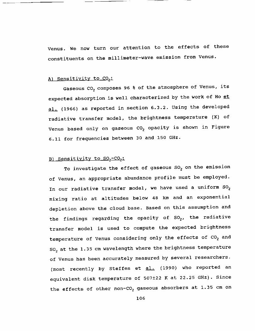
Venus. We now turn our attention to the effects of these
constituents on the millimeter-wave emission from Venus.
A) Sensitivity to COzl
Gaseous CO 2 composes 96 % of the atmosphere of Venus, its
expected absorption is well characterized by the work of Ho e_tt
al. (1966) as reported in section 6.3.2. Using the developed
radiative transfer model, the brightness temperature (K) of
Venus based only on gaseous CO 2 opacity is shown in Figure
6.11 for frequencies between 30 and 150 GHz.
B) Sensitivity to S02-C021
To investigate the effect of gaseous SO 2 on the emission
of Venus, an appropriate abundance profile must be employed.
In our radiative transfer model, we have used a uniform SO 2
mixing ratio at altitudes below 48 km and an exponential
depletion above the cloud base. Based on this assumption and
the findings regarding the opacity of SO2, the radiative
transfer model is used to compute the expected brightness
temperature of Venus considering only the effects of CO 2 and
SO 2 at the 1.35 cm wavelength where the brightness temperature
of Venus has been accurately measured by several researchers.
(most recently by Steffes et al. (1990) who reported an
equivalent disk temperature of 507±22 K at 22.25 GHz). Since
the effects of other non-CO 2 gaseous absorbers at 1.35 cm on
106

m
E
J
5OO
45O
400
35O
! i I I _ I
]CO 2 alone 1I .I
300 '20 40 60 80 100 120 140 160
Frequency (GHz)
Figure 6.11 Computed brightness temperature of Venus
assuming that gaseous CO z is the only atmosphericconstituent.
107
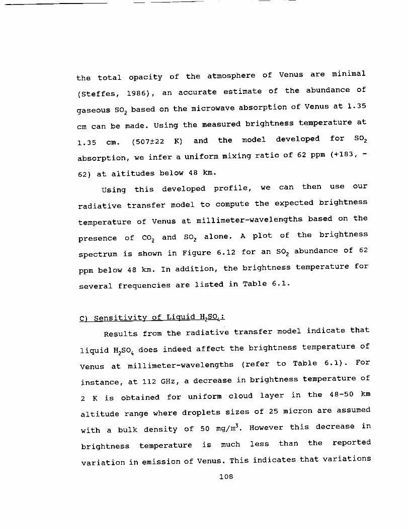
the total opacity of the atmosphere of Venus are minimal
(Steffes, 1986), an accurate estimate of the abundance of
gaseous SO 2 based on the microwave absorption of Venus at 1.35
cm can be made. Using the measured brightness temperature at
1.35 cm. (507±22 K) and the model developed for SO 2
absorption, we infer a uniform mixing ratio of 62 ppm (+183, -
62) at altitudes below 48 km.
Using this developed profile, we can then use our
radiative transfer model to compute the expected brightness
temperature of Venus at millimeter-wavelengths based on the
presence of CO 2 and SO 2 alone. A plot of the brightness
spectrum is shown in Figure 6.12 for an SO 2 abundance of 62
ppm below 48 km. In addition, the brightness temperature for
several frequencies are listed in Table 6.1.
C) Sensitivity of Liquid H2S__OI
Results from the radiative transfer model indicate that
liquid H2SO 4 does indeed affect the brightness temperature of
Venus at millimeter-wavelengths (refer to Table 6.1). For
instance, at 112 GHz, a decrease in brightness temperature of
2 K is obtained for uniform cloud layer in the 48-50 km
altitude range where droplets sizes of 25 micron are assumed
with a bulk density of 50 mg/m 3. However this decrease in
brightness temperature is much less than the reported
variation in emission of Venus. This indicates that variations
108

L_
c
45o ,-t
I
aO,5 -
L i
rI i500 ' ' '
25 40
COz+S02 ]
\
\\x
I 1 1 I
t
60 80 I00 120 140 160
Frequency (GHz)
Figure 6.12 Expected brightness temperature of Venus based
on the presence of CO 2 and SO 2 with an SO 2 abundance of 62ppm below 48 km and exponentfally decreasing above 48 km.
109
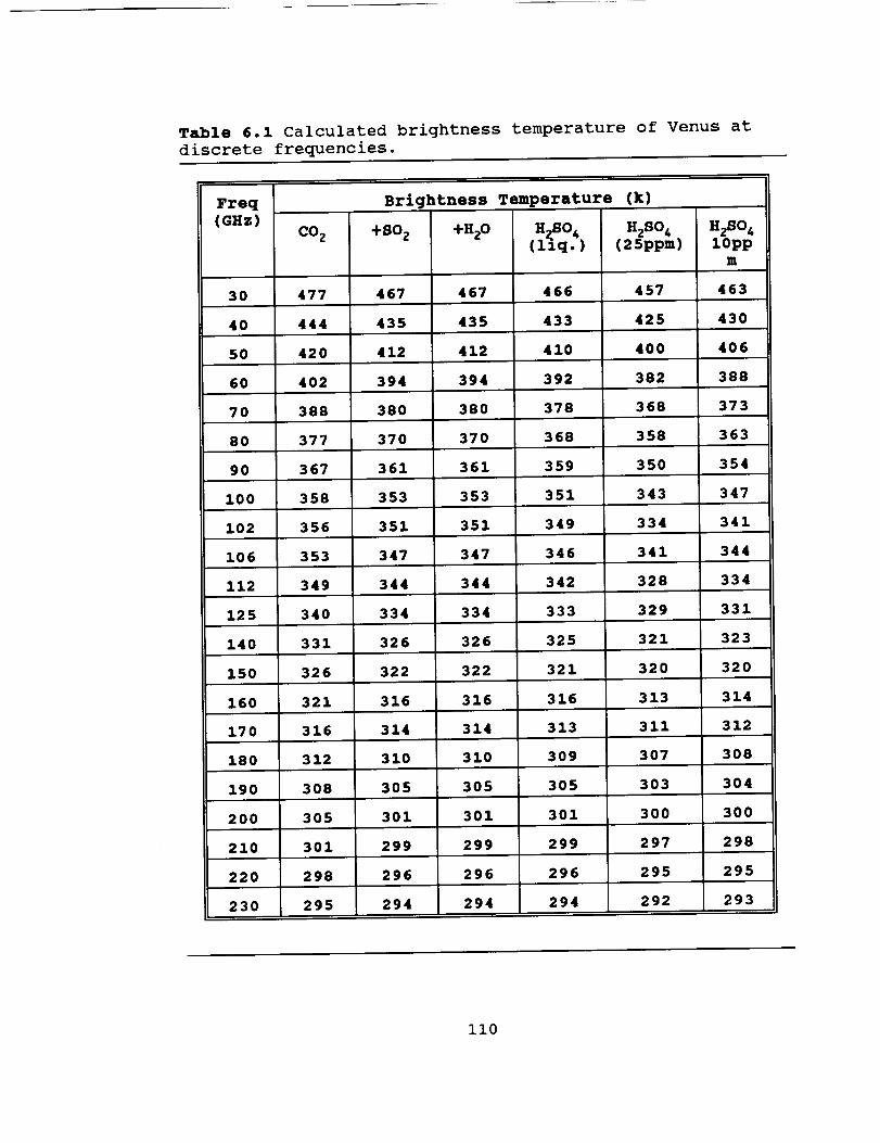
Table 6.1 Calculated brightness temperature of Venus at
discrete frequencies.
Freq Brightness Temperature (k)
(GHz) CO2 +802 +H20 H_ O4 H2804 H2804
(11q.) (25ppm) lOpp
m
30 477 467 467 466 457 463
40 444 435 435 433 425 430
50 420 412 412 410 400 406
60 402 394 394 392 382 388
70 388 380 380 378 368 373
80 377 370 370 368 358 363
90 367 361 361 359 350 354
100 358 353 353 351 343 347
102 356 351 351 349 334 341
106 353 347 347 346 341 344
112 349 344 344 342 328 334
125 340 334 334 333 329 331
140 331
326
326 326 325 321 323
150 322 322 321 320 320
160 321 316 316 316 313 314
170 316 314 314 313 311 312
180 312 310 310 309 307 308
190 308 305 305 305 303 304
200 305 301 301 301 300 300
210 301 299 299 299 297 298
220 298 296 296 296 295 295
230 295 294 294 294 292 293
ii0

in the abundance of liquid H2SO_ are not the major source of
the observed brightness temperature variations.
However, by using our model of the complex dielectric
constant of liquid H2SO4 and the radiative transfer model, we
have demonstrated that liquid H2SO4 does have an effect on the
millimeter-wave emission of Venus
presence must be included in any
emission of Venus.
(see Table 6.1) and its
future modeling of the
D) Sensitivity to H20 vapor:
The expected absorption of H20 vapor is included in the
radiative transfer model in order to study its effects on the
millimeter-wave emission of Venus. As a result, we have found
that water vapor has a minimal effect on the calculated
brightness temperature of Venus at millimeter wavelength (see
Table 6.1). A plot of the computed brightness temperature of
Venus with CO2, SO 2 and H20 is shown in Figure (6.13) using an
abundance profile of 70 ppm at 30 km and an abundance that
decreases linearly above and below 30 km.
E) Sensitivity to H2S__O vapor:
The expected opacity of gaseous H2SO 4 in a CO 2 atmosphere
is also included in the radiative transfer model. This opacity
is based on the VVW model of H2SO 4 absorption as discussed in
Chapter 5. An abundance profile of 25 ppm between 38 and 48 km
iii

E
mw
500 ! i ] i
i C02_S02_H20 ]
20 z, T: 6,5 gO, ', ,,%_3 : 20 ] a0
Frequency (GHz)
6%
Figure 6.13 Calculated brightness temperature of Venus based
only on CO 2, SO 2 and Water vapor.
112

is also used in our model. (This abundance of H2SO4 gas is
based on the work of Jenkins and Steffes (1991), who reported
average abundances on that order for the equatorial regions of
Venus based on Pioneer Venus radio occultation studies. Note,
however, that they reported abundances variations from 0 to 30
ppm, depending on location.) Above 48 km, the abundance
profile follows the saturation abundance of H2SO4 as determined
from the T-p profile of Venus and the partial pressure of H2SO4
(see appendix A). Below 38 km, the abundance is assumed to be
zero.
A plot of the resulting brightness temperature spectrum
of Venus between 30 and 230 GHz is shown in Figure (6.14),
where a comparison between the brightness temperature with
H2SO4 abundance of 25 and i0 ppm is shown.
F) Millimeter-wave spectra of Venus:
A plot of the calculated millimeter-wave spectrum of
Venus based on the presence of one or more constituents is
shown in Figure (6.15) for frequencies between 30 and 230 GHz.
The abundance profile of each constituent used to develop this
brightness temperature profile is summarized in Table 6.2.
A closer examination of the reported spectrum of Venus
reveals several important features:
113

500
4-75
425
o
e.g
_" 325
Brightness Temperature of Venus
10 ppm
ppm
'-, _-,O 1O0 150 200 250
Frequency (GHz)
Figure 6.14 Calculated brightness temperature of Venus for
H2SO 4 abundances of 25 and i0 ppm for frequencies between 30and 230 GHz.
114

500
p -e-
r- ,r--_E 4u_c,,;
U':,
.2
ziU ¸_
CO z
.__ +S0 z
..... +H20\\ i ......... +Liq HzSO 4
_< ......... +HzS04 gas
.?..,,
" -7",,; t" _..,.._?,,_
: / ::bt_.,,_.
• t/ 'v "_,-_,_
'3 50
' P , L , _ ] , :
IO0 150 200 250
Frequency (GHz)
Figure 6.15 Comparison of the effects of atmosphericconstituents on the brightness temperature of Venus between
30 and 230 GHz.
115

Table 6.2 Abundance profiles for each of the constituents
present in the atmosphere of Venus.
Atmospheric Constituents Abundance Profile
CO?
Gaseous 802
Water Vapor
H2SO , (liquid)
Gaseous HzSO 4
96 % and 3% N 2
62 ppm below 48 km and
exponentially decreasing
above 48 km.
70 ppm at 30 km. and
decreases linearly below
and above 30 km.
85% concentration by
weight. Droplets diameterof 25 microns and a bulk
density of 50 mg/m_.
25 ppm between 38 and 48
km, zero ppm below 38 km.Abundance follows
saturation abundance above
48 km.
a) Gaseous SO 2 does affect the brightness temperature of
Venus. However, variations in its abundance cannot completely
account for the measured 30 K variation in emission measured
by de Pater et al. (1991). In addition, gaseous SO 2 seems to
have the biggest effect on the brightness temperature at
frequencies below 180 GHz as noted in Table 6.1. This
frequency dependence of the change in brightness temperature
can be well explained by carefully examining Figures 6.16 and
6.17 which show the weighting functions of the atmosphere of
Venus at several frequencies. (Note that the abrupt
discontinuities in the weighting function are due to the
116

,m
0.07
006
0.05
0.0 4
0. ,3}
O.C2
¢::. 0 1
O.OO
-0.0i
, 1 I
-- 30 GHz
--- 50 GHz
..... 75 GHz
......... 100 GHz!
........ 102 GHz!i
::s o: '-*:o it t
t 1; _ : .
i/
I no . i ', ".: It '.'.
I : _ ','.
/ " / ;'X..,,I ,, ..;/ / : :.-.,-,\_ ,,',..
/ / ,, ...'/ \ \ ,,',,
0
I i
mc3' 40 60
Altitude (KM)
Figure 6.16 Calculated weighting functions of the atmosphereof Venus as function of altitude at 30,50,75,100 and 102
GHz.
117

=
J
_t
0.07
:: $ E
C:.CO
I _ i i i
-:, £,:-"3: 5 0 60 7 0
Altitude (KM)
Figure 6.17 Calculated weighting functions of the atmosphereof Venus as function of altitude at 112, 125, 143, 160, 180,
230, 260 GHz.
118

addition of one or more atmospheric constituents.) Also note
that at frequencies below 180 GHz, most of the emission from
the atmosphere of Venus is emanating from a portion of the
atmosphere where gaseous SO 2 is abundant, in this case below
48 km. At frequencies above 180 GHz, the weighting function
shifts up in altitude which means that the emission is due to
the absorption of the constituents present above 50 km,
predominately gaseous CO 2.
b) The addition of water vapor to SO 2 and CO 2 has little effect
on the brightness temperature of Venus. This is indicated by
the fact that the brightness temperature profile of Venus with
SO 2 and CO 2 alone completely overlays the brightness
temperature profile obtained when water vapor is added (see
Figure 6.15).
c) The presence of liquid sulfuric acid as a cloud condensate
does have an impact on the calculated brightness temperature
of Venus as shown in Table 6.1. Specifically, for frequencies
between 30 and 120 GHz, a drop of 2 K is observed due to the
addition of H2SO 4 condensate to the atmosphere of Venus.
Between 120 and 150 GHz, a drop of 1 K is observed. Above 150
GHz, the drop in the brightness temperature is barely
noticeable. This effect is also noticed in Figure 6.15 where
a complete overlay of the brightness spectra with and without
119

liquid sulfuric acid
GHZ.
is observed at frequencies above 150
d) Aside from gaseous C02, gaseous H2SO 4 seem to have the
biggest effect on the calculated brightness temperature of
Venus. Specifically at 112 GHz, the brightness temperature
with CO2+SO2+H2SO_(Iiq)+H20 is 342 K. When gaseous H2SO 4 is added
to the atmosphere of Venus, a drop of 14 K is observed (see
Table 6.1). However, at 106 GHz, a drop of only 5 K is
obtained. This abrupt change in the brightness temperature
between 106 and 112 GHz can be easily explained by the shape
of the absorption profile of gaseous H2SO 4 reported in Figure
6.9. From this profile, we see that at 112 GHz the absorption
goes through a local maximum which tend to greatly decrease
the calculated brightness temperature. At 106 GHz, the profile
goes through a local minimum which yields a smaller change in
the brightness temperature of Venus. This phenomenon is quite
noticeable for frequencies between 50 and 180 GHz where
several "dips" in the calculated brightness temperature are
observed. Above 180 GHz, the magnitude of these dips decrease
and the effect of the presence of gaseous H2SO 4 in the
atmosphere on the brightness temperature is minimized. This is
consistent with the weighting function at 180 GHz which shows
that most of the emission is emanating from altitudes above 50
km. Thus, at frequencies above 180 GHz, most of the observable
120

absorption in the atmosphere of Venus is due to the presence
of gaseous CO2.
e) Comparisons with radio observation of Venus:
Although many researchers have observed the radio
emission from Venus at microwave frequencies (Steffes et al.
1990, Janssen and Poynter, 1981), very few have observed the
emission from Venus at millimeter-wavelengths, de Pater et al.
(1991) observed the millimeter-wave emission of Venus at 112
GHz and their observations showed a variation of 30 K in the
emission between the night and day side of Venus.
Table 6.3 Comparison between observed and computed brightness
temperature of Venus.
Frequency (GHz) Computed Observed
Brightness Brightness
Temperature (k) Temperature (k)
13.3 557 561_191
18.46 519 520±171
22.2 499 507±221
112.2 3282,3433 Max=365 a Min=335 a
I Steffes et al. 1990.
2 25 ppm H2SO 4
3 0 ppm H2SO 4a de Pater et al. 1991.
121

Table 6.3 summarizes recent observations of Venus. The
observed emissions are also compared with our calculated
brightness temperature from the radiative transfer model. The
results reported in Table 6.3 indicates that our radiative
transfer model agrees with the measured values. This is quite
important since we can now state that the observed variations
by de Pater et al. (1991) are most likely due to variations in
the abundance of gaseous sulfuric acid and not to liquid
sulfuric acid as previously suggested.
122

CHAPTER 7
SUMMARY AND CONCLUSIONS
7.1 Uniqueness of Work
This research provides new information which is essential
to the understanding of the millimeter-wave spectrum of Venus.
In addition, this research provides contributions to both
planetary science and millimeter-wave measurement techniques.
In the laboratory measurements area, our measurement of the
dielectric constant of liquid sulfuric acid represents the
first time that its absorption coefficient has been determined
at millimeter-wavelengths. The results of the measurement of
the opacity of SO 2 under Venus-like conditions are very
significant in that they present the first time that the
opacity of sulfur dioxide has been measured at millimeter-
wavelengths under simulated Venus conditions. In addition, our
results have shown that the f2 dependence of the opacity of SO 2
123

is not valid and that the Van Vleck-Weisskopf formalism seems
to accurately model the opacity of SO2 at frequencies above 20
GHz. As a result, an updated abundance profile of SOz has been
determined. The measurements of the dissociation factor of
H2SO 4 have provided a direct technique for measuring the
partial pressure of gaseous sulfuric acid. The results from
the latter measurements are used to determine the saturation
abundance of H2SO 4 in the atmosphere of Venus. Finally, our
measurement of the millimeter-wave opacity of gaseous H2SOJCO _
under Venus-like conditions represents the first laboratory
measurement of the opacity of this gaseous mixture at 94 GHz.
Several contributions toward microwave and millimeter-
wavelength measurement techniques have resulted from our
research. This includes an innovative technique of measuring
the opacity of a gaseous mixture while minimizing the effects
of dielectric loading on the quality factor of the resonator
used. In addition, the measurement of the dielectric constant
of liquid sulfuric acid has demonstrated the ability of a free
space transmission system for conducting such measurements.
Although the development of the radiative transfer model
is not entirely new, the incorporation of our measured results
into the model provides for the first time the ability to
accurately interpret the millimeter-wavelength emission of
Venus. Results of the radiative transfer model indicate that
gaseous SO 2 does have a significant effect on the emission of
124

Venus. In addition, the presence of H2SO4 cloud layer does
affect the emission of Venus in that the cloud effect is
comparable with that of gaseous SO2. However, we have found
that the presence of SO2 and liquid H2SO4 cannot completely
account for the measured variations in the observed emission
at 112 GHz. Another important finding is that water vapor does
not significantly affect the emission at millimeter-
wavelengths. Lastly, we have demonstrated that variations in
the abundance of gaseous sulfuric acid is the most likely
the measured variation in the millimeter-wavecause of
emission.
These
observations
results, in conjunction with the reported
of Venus, have allowed us to develop a new
abundance profiles for the atmospheric constituents of Venus.
Revised limits on the abundances of gaseous SO2 and H2SO4 have
been determined. This type of information is crucial in the
development of theories regarding the evolution of Venus which
in turn may help in the study of planet earth.
Finally, this research has resulted in the publication of
two papers:
i) Fahd, A. K., and P. G. Steffes, Laboratory measurements of
the millimeter-wave properties of liquid sulfuric acid (H2SO4) ,
J. Geophysical Research : Planets, 96, E2, 17471-17476, 1991.
125

2) Fahd, A. K., and P. G. Steffes, Laboratory measurements of
the opacity of gaseous sulfur dioxide under Venus-like
conditions, Icarus, accepted for publication, March, 1992.
In addition, this research has been presented as several
conference reports:
i) A.K. Fahd and P.G. Steffes, "Laboratory Measurements of the
Opacity of Gaseous Sulfuric Acid (HzSO4) at 94 GHz.", Bulletin
of the American Astronomical Society, vol. 22, 1991.
Presented at 23rd Annual Meeting of the Division for Planetary
Sciences of the American Astronomical Society, Palo-Alto,
November 4,1991.
2) A.K. Fahd and P.G. Steffes, "Laboratory Measurements of the
Opacity of Gaseous Sulfur Dioxide (SO2) at 94 GHz," Bulletin
of the American Astronomical Society, vol. 22, 1991.
Presented at 23rd Annual Meetinq of the Division for Planetary
Sciences of the American Astronomical Society, Palo-Alto,
November 4, 1991.
3) A.K. Fahd and P.G. Steffes, "Laboratory Measurements of the
Millimeter-Wave Properties of Liquid Sulfuric Acid (H2SO4)
Between 90 and I00 GHz," Bulletin of the American Astronomical
society, vol. 22, pg. 1035, 1990.
126
Presented at the 22nd Annual Meeting of the Division for
Planetary Sciences of the American Astronomical Society,
Charlottesville, Virginia, October 22, 1990.
4) A.K. Fahd and P.G. Steffes, "Laboratory Measurements of the
1.3 and 13.3 cm Opacity of Gaseous SO 2 under Simulated
Conditions of the Middle Atmosphere of Venus," Bulletin of the
American Astronomical Society, vol. 22, pg. 1032, 1990.
Presented at the 22nd Annual Meeting of the Division for
Planetary Sciences of the American Astronomical Society,
Charlottesville, Virginia, October 22, 1990.
5) A.K. Fahd and P.G. Steffes, "Laboratory Measurements of the
Dissociation Factor of Gaseous Sulfuric Acid (HzSO4)," Bulletin
of the American Astronomical Society, vol. 21, pg. 927, 1989.
Presented at the 21st Annual Meeting of the Division for
Planetary Sciences of the American Astronomical Society,
Providence, Rhode Island, November i, 1989.
7.2 Suggestion for Future Work
Although we are in a better position to explain the
observed variation in the millimeter-wave emission from Venus,
several important ideas can be further explored to better
understand the millimeter-wave spectrum of Venus:
127

A) Conduct a more accurate measurement of the temperature
dependence of the opacity of gaseous S02: This can be achieved
by conducting laboratory measurements using a configuration
similar to the one described in this work but at different
temperatures (specifically, at a range of temperatures that
are characteristic of the atmosphere of Venus). As a result of
this proposed measurement, one could develop a more accurate
temperature dependence for the SO2 opacity, and hence a better
estimate on the abundance of sulfur dioxide in the atmosphere
of Venus.
B) Develop a laboratory apparatus to be used in conjunction
with a mass spectrometer to investigate the presence of
gaseous H2SO4 dimers at certain pressures and temperatures. The
presence of these dimers can greatly influence the measured
partial pressure of gaseous H2SO4 which can yield to erroneous
determination of the saturation abundance of gaseous H2SO4 in
the atmosphere of Venus (see Appendix A).
C) Conduct radio observations of the emission of Venus at 112
and 106 GHz so as to confirm the presence of the reported
"dip" in the brightness temperature of Venus as reported in
Chapter 6.
128

D) Development of a Fourier Transform Spectrometer which can
be mounted on existing millimeter and submillimeter antennas.
The development of such an apparatus will make it easier to
study broad spectral features of Venus.
129

APPENDIX A
A.1 Measurement of the Vapor Pressure of Sulfuric Acid (H2804)
The apparatus developed for the measurement of the
dissociation factor of gaseous sulfuric acid is shown in
Figure A.I. In this setup, a large chamber (of known volume,
in this case 34.8 Liters) was constructed using Pyrex glass as
shown in Figure A.2. The reasons for choosing glass are its
ability to withstand high temperatures in addition to the
ability of monitoring the status of the sulfuric acid vapor to
make sure that the vapor does not condense during the pressure
measurement. The top of the glass vessel is sealed using a
stainless steel plate. In order to form a good seal at the
glass lip, a high temperature Viton O-ring is sandwiched
between the glass and the plate.
Throughout the setup, stainless steel tubes are used to
minimize the acid-metal reaction at high temperatures. In
addition, all stainless steel tubing was submerged in a
sulfuric acid solution for an extended period of time prior to
the experiment. This process helped minimize the amount of
impurities (within the stainless steel tubing) which could
130

<
ILl
CC_
E
%D
_D
z
c__
c
z
£Do%c_
_ m m
I
U_..J
C_
O
O
C_
-r
II
i
\£.J
_<_%D<
7I
Y
\ Z
_-c<c
c._
Figure A.1 Laboratory apparatus used to measure thedissociation factor of gaseous sulfuric acid.
131

O
Z
Figure A.2 Cross sectional view of the vacuum chamber used in
the setup.
132

react with the sulfuric acid producing inaccurate results. A
custom made Pyrex flask was designed so that the liquid
sulfuric acid could be introduced and extracted from the
system with ease. The flask is filled with a precisely known
volume of liquid sulfuric acid at room temperature where for
volumes less than 1 ml, repeatable accuracies of better than
.01 ml have been obtained.
The complete system is contained inside a temperature
controlled oven. The system employs two vacuum gauges, P1 and
P2 where gauge P1 is used to measure pressures in the 0-20
Torr range while gauge P2 is used to measure pressures ranging
from 0 to 800 Torr with 1 Tort increments. A small amount of
nitrogen is used in the experimental setup as a buffer so as
to prevent any sulfuric acid vapor from coming in direct
contact with gauge P2. The laboratory measurements were
conducted on two different concentrations of liquid sulfuric
acid (99% and 95.9% by weight) at distinct temperatures
ranging between 480 to 603 K (Table A.I).
The measurement procedure can be summarized as follows:
The oven is first heated to the desired temperature. Once this
temperature is reached, the chamber is evacuated. By using
gauge P1 as a vacuum monitor, we are able to check the status
of the vacuum chamber in order to insure that no major leaks
are present. Although no leak-proof vacuum was obtained, we
were able to maintain a leak rate within the system of less
133

than .8 Tort/hour. The minimization of these leaks has a major
effect on the calculation of the dissociation factor since any
substantial leaks in the system can alter the measured
pressure. The nitrogen buffer valve is then opened and the
resulting pressure (due only to nitrogen gas) is recorded. The
system is then evacuated and the buffer is refilled with equal
amount of nitrogen. The remaining nitrogen in the system is
evacuated and the flask (containing liquid sulfuric acid)
valve is opened allowing the sulfuric acid liquid to reach
vapor pressure equilibrium with the evacuated chamber. Once
equilibrium is reached, the flask valve is closed and a visual
check is made to verify that the remaining liquid acid is
clear. After the flask is closed, the valve connecting gauge
P2 (containing a small amount of nitrogen as a buffer) is
opened and the system is allowed to reach equilibrium. The
resulting chamber pressure is then recorded.
Throughout this process, the system temperature was
maintained to within ± 5 K so as to minimize the effects of
temperature variation on the results. Once the chamber
pressure was recorded, the oven was shut off and the gaseous
sulfuric acid was evacuated from the chamber. The system is
then allowed to cool overnight to its original room
temperature. At that point, the remaining volume of liquid
sulfuric acid is measured and the evaporated liquid volume is
determined.
134

1%.2 Determination of the Dissociation Factor and the Partial
Pressure of Gaseous Sulfuric 1%¢id (H2SO 4)
The dissociation factor of gaseous H2SO 4 can be inferred
from a number of quantities actually measured during the
experiment. Let VLi_i d (ml) denote the volume (at room
temperature) of liquid HzSO 4 and liquid HzO (since we are not
using a 100 % concentration by weight) that evaporates from
the flask during the experiment. Thus, VLiquid can be expressed
as a function of VHZ 0 and VHzSO4 ,
vLi_ d = _ (v._so" , v._o) (1%.i)
The percent concentration of the liquid sulfuric acid (by
weight) can be defined as follows:
PCM = Vzy's°'P_2s°4 (1%.2 )
V.,so. P+,_so,+ V,_o P_,o
(i.e. PCM=.99 for 99 % concentration by weight), where PHzO is
the density of H20 (i g/ml) and P,2s04 is the density of liquid
sulfuric acid. From equations (A.I) and (A.2) one can solve
for VH20 and V,2s04,
V_r2° = Vl.iquid PZ.iqluid(1 -PCM) (i%.3 )
P H2o
and
135

V".so_ = VLi_i _ PCM PLi_idPH2so,
(A.4)
where PLiquid is the density of the liquid mixture. Thus by
using equations (A.3) and (A.4) one can calculate the volume
of liquid HzSO 4 and liquid HzO that evaporated from the liquid
solution. This calculation is necessary since the liquid
solution used in the experiment is not i00 % sulfuric acid and
any additional pressure that is due to dissolved water must be
accounted for. The pressure due to the vaporized liquid water
can be found by calculating the number of evaporated moles and
using the ideal gas law as follows,
PH_o (A.5)_Watez = VH20 16
where _,ateris the number of the evaporated moles of water. The
pressure due to _.ater ' Pwater(atm)' can then be calculated from,
Pwa tez - 11wacer R T (A. 6 )Vchambe r
where R is the ideal gas constant (.08205 i. Atm/mole K.), T
is the temperature of the chamber in K and Vcha_ r (liters) is
the volume of the vacuum chamber.
The net pressure expected from the evaporated sulfuric
acid molecules (PNet)' can be written as,
PNe_ =PResult - Pwa_ez -PNi_rogen (A.7)
136

where PResult is the measured pressure from gauge P2 and PNitrogen
is the pressure in the system due only to the nitrogen buffer.
Thus P,et can be thought of as the pressure due to H2SO 4 and any
additional SO 3 and H20 molecules that dissociate from the
evaporating sulfuric acid. As a result, equation (A.7) can be
written as,
where P,2 0 in equation (A.8) is a different quantity than that
determined in equation (A.6). The application of the ideal gas
equation to PNet yields,
PNet Vchamber = 11Total R T (A. 9 )
where _Totat is the total number of moles of gas that result
from the evaporated sulfuric acid liquid. It can be written
as,
_To_al = _H2SO 4 (I+D) (A.10)
where _,2s04 is the number of moles of liquid sulfuric acid
which vaporized while the flask was open and D is the
dissociation factor defined as,
D : Pso, (A. 11)
PH2so, + Pso,
The quantity U,2s04 can be obtained from the volume of the
liquid sulfuric acid and its density,
137

P,2so, (A. 12 )I]H2SO" = V_2S04 98
The determination of the dissociation factor can then be
calculated using equations (A.4,A.9,A.10,A.12) ,
9 8 P_;,T Ve_w_,z (P_ + P;%so4 (1 - PCM ) ) - ( VLi_.jid PC_4 P_o. R 7")m = (A. 13)VL_i d PC_ Pz%9o. R T
Thus if the chamber volume, the system temperature, the
density of liquid sulfuric acid, the pressure resulting from
the evaporated liquid acid, and the amount of the evaporated
liquid are known, then a direct application of equation (A.13)
will give the dissociation factor of the gaseous sulfuric
acid. Once the calculated dissociation factor D is determined,
the partial pressure of gaseous HzSO 4 can then be calculated.
This can be performed by using equation (A.8) and the fact
that P,z0 is equal to Ps03,
PN.t= PH.so.÷ 2 Pso.= P,.so.÷ 2 P,_o (_.14)
by combining equations (A.II) and (A.14), the partial pressure
of gaseous HzSO 4 (P,2s04) can be written as,
PNet ( 1 - m ) (A. 15)PH_so, = ( 1 + D )
Thus the partial pressure of gaseous sulfuric acid can be
computed from equation (A.15) provided that the net pressure
measured and the resulting dissociation factor are known. For
138

the special case when the dissociation factor is unity,
equations (A.10) and (A.12) yield,
PN_:= 2 Pso3= 2 PH_o (A. z6)
Another important quantity that is used in the literature
(Gmitro and Vermeulen, 1964) is Kp which is known as the
equilibrium constant and it is defined as,
Pso, P,,o (_,. z_,)K, -
In order to use our results to calculate the equilibrium
constant of gaseous sulfuric acid, we need to express Kp as a
function of the dissociation factor and the partial pressure
of gaseous sulfuric acid. A direct manipulation of equations
(A. II) and (A.17) yields,
D2 PH2s°4 D _ 1 (A. 18)Kp = ( 1 -m) 2
Using equation (A.18) one can calculate the equilibrium
constant from our inferred dissociation factor and our
inferred partial pressure of gaseous H2SO 4. This calculation
serves as a comparison between our results and the ones
reported by Gmitro and Vermeulen (1964) and it can used in
correcting the partial pressure of H2SO 4 at temperatures below
480 K which were reported by Ayers et ai.(1980).
139

A.3 Measurement Results
Measurements were carried out on two liquid H2SO _ samples,
each having a different concentration. Measurements were
conducted at six distinct temperatures ranging from 480 to 603
K. The lower temperature point is dictated by the sensitivity
of the gauge P2 and its ability
pressures below 1 torr while the
temperature range is dictated by
to accurately measure
upper bound on the
the maximum allowable
temperature of the oven and the ability of some parts in the
system to withstand these high temperatures.
The partial pressure of gaseous H2SO 4 (99%, by weight)
is shown in Figure A.3. In this figure, the illustrated points
are results from the laboratory measurements (including error
bars) while the solid line is a best fit model of the data
according to the Clausius-Clapeyron model. From the best-fit
model, the vapor pressure of gaseous sulfuric acid for
temperatures between 480 and 603 K can be written as,
In p = 6.65 6100 (A.19)T
where p is the sulfuric acid vapor pressure (atm) and T is the
temperature in K. A similar result is obtained for 95.9%
concentration and is shown in Figure A.4. A best fit
expression for the latter concentration is given by,
140
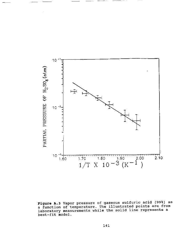
E
o_O9
O
5_
D-
<
<
0 _1-v
T
10 -2.
_o-' ,,,, ..... ,,..,,,,,,.- ........ ,.,,,, ,_.,,_,,,,,,,,1.60 1.'70 1.80 1.90 2.00 2.10
1/T X 10 -3 (K -1 )
Figure A.3 Vapor pressure of gaseous sulfuric acid (99%) as
a function of temperature. The illustrated points are from
laboratory measurements while the solid line represents abest-fit model.
141

V
O59
O
59
<
<
10 -I
10 -2.
0 _ I J I I J 1 I I I _ I I 1 I J i I i I 1 I I 'i ] I L ] I I I J I J I J l I i I i _ I i I | I i | |
1.60 1.70 1.80 1.90 2.00 2.
x lo.3 (k -1)0
Figure A.4 Vapor pressure of
as a function of temperature.
from laboratory measurementsa best-fit model.
gaseous sulfuric acid (95.9%)The illustrated points are
while the solid line represents
142

in p = 5.25 5430 (A.20)T
A careful examination of the two figures reveals that the
best-fit expression agrees with the measured data except for
temperatures above 590 Kelvins where a deviation from the best
fit model is observed. The laboratory measurements seem to
indicate that a saturation effect is occurring at these high
temperatures while our best fit model indicates a further
increase in the partial pressure of gaseous sulfuric acid with
temperature. This observed phenomenon is not yet fully
understood but one can speculate that the Clausius-Clapeyron
model may not be valid for these temperatures and an alternate
model may be required (additional discussion regarding this
effect is presented later in this Appendix).
A comparison between our expressions and the ones
reported by Steffes(1985), Ayers et al., (1980) and Gmitro and
Vermeulen (1964) is shown in Figure A.5. An examination of
this figure reveals that Steffes overestimated the partial
pressure for high temperatures while he underestimated the
partial pressure for temperatures below 510 K. This deviation
may be attributed to the fact that Steffes did not measure the
dissociation factor but he assumed a 47% dissociation factor
over the measured temperature range. The comparison between
our results and the extrapolation of the results reported by
Ayers et al. shows that their expression overestimates the
143
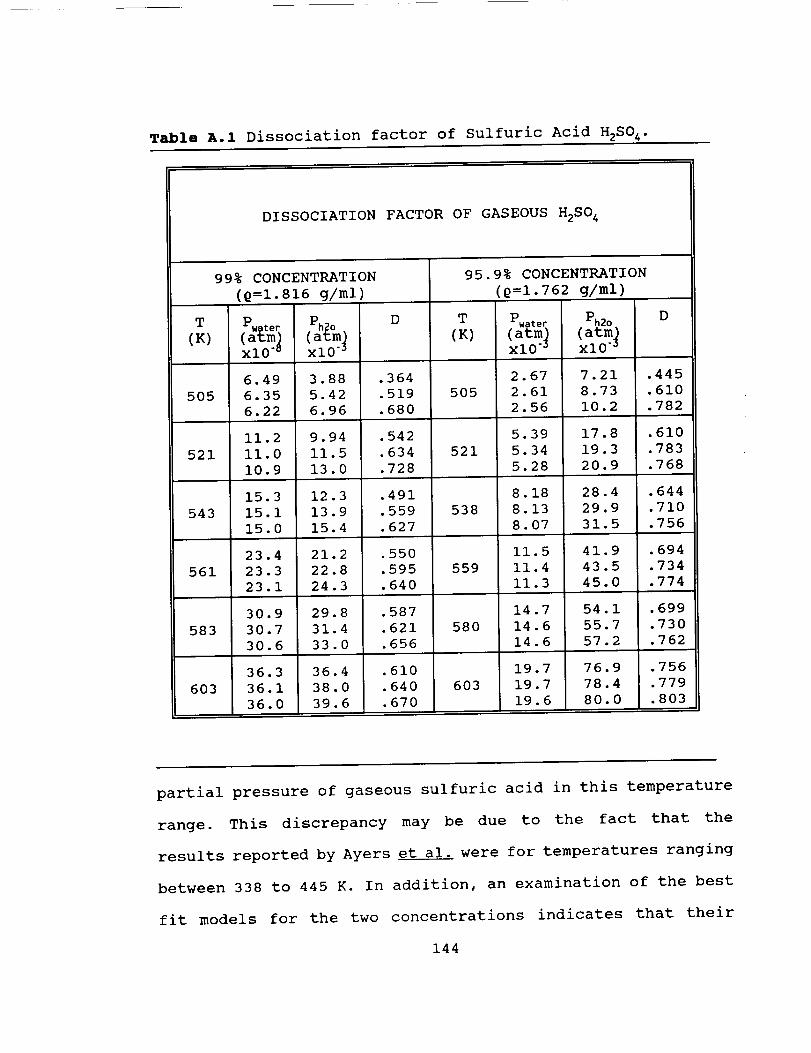
Table A.I Dissociation factor of Sulfuric Acid H2SO_.
DISSOCIATION FACTOROF GASEOUSH2SO4
T(K)
505
99% CONCENTRATION
(Q=1.816 g/ml)
D
Pwater (Pah_(atm_xl0 TM xl0 TM
6.49 3.88
6.35 5.42
6.22 6.96
11.2 9.94
ii.0 11.5
10.9 13.0
15.3 12.3
15.1 13.9
15.0 15.4
23.4 21.2
23.3 22.8
23.1 24.3
30.9 29.8
30.7 31.4
30.6 33.0
36.3 36.4
36.1 38.0
36.0 39.6
.364
.519
.680
.542
.634
.728
95.9% CONCENTRATION
(Q=I. 762 g/ml)
T
(K)
5O5
Pwater
(atm_xl0 TM
2.67
2.61
2.56
5.39
5.34
5.28
Ph2o
(atm_XI0 TM
7.21
8.73
10.2
17.8
19.3
20.9
D
.445
.610
.782
.610
.783
.768
521 521
•491 8.18 28.4 .644
543 .559 538 8.13 29.9 .710
.627 8.07 31.5 .756
.550 11.5 41.9 .694
561 .595 559 11.4 43.5 .734
.640 11.3 45.0 .774
•587 14.7 54.1 .699
583 .621 580 14.6 55.7 .730
•656 14.6 57.2 .762
.610 19.7 76.9 .756
603 .640 603 19.7 78.4 .779
•670 19.6 80.0 .803
partial pressure of gaseous sulfuric acid in this temperature
range. This discrepancy may be due to the fact that the
results reported by Ayers et al. were for temperatures ranging
between 338 to 445 K. In addition, an examination of the best
fit models for the two concentrations indicates that their
144

-TO
O
<
<
I0
m
0 _I,
Gmitro &
__ Vermeulen
]0 -2.
Steffes"'-._'Ayers et a].
This / -__-_
(99 Z)" /
(95.9 %)" -"
0 _ i _1 1 111_7]]1111;lltl I I]11;11111tll I III IIIl11111111 I I I I I I ] 11
1.50 1.60 1.70 1.80 1.90 2.00 2.10
X o-a(K
Figure A.5 Best-fit expression of the H2SO 4 partial pressure(solid line) of our data in comparison with the results of
Steffes (1985), Ayers et al. (1980), and Gmitro and
Vermeulen (1964).
145

slope did not change with acid concentration which suggests
that the partial pressure is directly related to the
concentration of liquid sulfuric acid. Thus as the
concentration of the acid decreases so does its vapor
pressure.
The resulting values of the dissociation factor for both
liquid concentrations calculated from our measurement are
listed in Table A.I. These values are obtained from the
measured pressure and the volume of liquid that evaporated
during the measurement by using equation (A.13). In addition,
Table A.I lists the calculated values of Ph2o and Pwateras
determined from our measurements. The upper and lower values
of the dissociation factor and calculated pressures presented
in this table include uncertainties due to the pressure
reading in addition to uncertainties in the evaporated liquid
volume.
To use the above results in the determination of the
saturation abundance and mixing ratio of gaseous sulfuric acid
in the atmosphere of Venus, we must evaluate the partial
pressure of H2SO4 at lower temperatures (330 to 480 K). A
Direct extrapolation of our results to lower temperatures may
not be valid since the actual partial pressures often deviate
from the Clausius-Clapeyron model. Since the laboratory
measurements by Ayers et al. were conducted in a more
appropriate temperature range (338-445 K), we instead apply
146

our results for the equilibrium constant Kp to the Ayers e__t
al. data in order to recalculate a new partial pressure. (This
is because these authors had previously used a theoretically
derived value for the equilibrium constant for deriving the
partial pressure). This process requires the calculation of a
best-fit expression for the equilibrium constant according to
our measurements which can be written as,
where KP
3925log kp = + 8.33 (A.21)
T
is in Torr and T is the temperature in K. A plot of
the above result compared with the result reported by Gmitro
and Vermeulen (1964) is shown in Figure A.6. In this figure,
the dashed line represents a best fit model for Kp as reported
by Gmitro and Vermeulen, the illustrated data points are the
calculated values for Kp from our laboratory measurements, and
the solid line is a best-fit model to our data as given in
equation (A.21) (In the calculation of our best-fit
expression, the effect of the equilibrium constant at 521 K on
the model was not included. The exclusion of this data point
is mainly due to the high value of the dissociation factor
observed at that temperature point as seen in Table A.I). In
order to compute the partial pressure at temperatures between
330 and 480 K, we need to extrapolate the best fit model to
cover that temperature range. The results of this
extrapolation are shown in Figure A.7 where the dashed line
147

O
O
2.50 w
m
- \ Gmitro &2.00 - x
\ x/Vermeulen
1.50 : \
1.0o This Work - _T
0.50 ! _"
0.00 I,,, ......,......_,,i .....,,,,,.........1.........J,,,,.....
1.50 1.60 1.70 1.80 1.90 2.00 2.
1/T X 10-3(K -:1)
0
Figure A.6 Comparison between our best-fit expression for
the equilibrium constant and the data reported by Gmitro and
Vermeulen (1964). Error bars due to temperature and pressure
are shown.
148

4.00
2.00
"_" 0.00i-,t,,,-0
[.-
-2.00
::x::
_.0
o -4.00
w
a
,,,,,.,d
Gmitro &len
This %'ork _ \_
\
-6.00
-8.001
i I I t I 1 1 I 1 I t l I l 1'1 I i I I I I 1 1 I I I I t I I I Ill I I i I 11 1 111 I I i I I
.20 1.60 2.00 2.40 2.80 3.20
I/T x lO-3(k --1)
Figure A.7 Comparison between our best-fit
equilibrium constant and the data reported
Vermeulen (1964) between 330 and 603 K.
expression for the
by Gmitro and
149

represents the extrapolation of the data reported by Gmitro
and Vermeulen and the solid line represents the extrapolation
of our best-fit model. A comparison of the two best-fit lines
reveals that a noticeable difference between the two
respective values of the equilibrium constant is observed.
As stated, the computation of the partial pressure of
H2SO4 for temperatures between 330 and 480 K requires the
correction of the data reported by Ayers et al. (1980) using
the new values of Kp. This process requires the calculation of
the total vapor pressure indicated by Ayers et al. (which was
not presented in their paper) and the recalculation of the new
partial pressure of gaseous sulfuric acid using the new K p
values. The values of the water vapor pressure used in this
calculation were from the data reported by Gmitro and
Vermeulen since they did not greatly differ from the one
measured in our experiment (480 to 603 K) and were also used
by Ayers et al. . The resulting best-fit expression for the
partial pressure of gaseous H2SO 4 (in the 330 to 480 K range)
using our values for Kp can be expressed as ,
in p = 10331 + 16.4 (A.22)T
where p is the pressure
temperature in Kelvins.
A complete plot of the
in atmospheres and T is the
partial pressure of gaseous
sulfuric acid as a function of the temperature is shown in
150

10 -I
a
,,_ 10 -.:
(Dr..,o
10-z,:=::
O
-- o10'
5050
tw,0....
<
[-._x
Laboratory
,_ Ayers et
10-_. Corrected d"_aX /
\ \,,"--.X,10 "_" "" "_\
10 -./1 ' _' ' I _ ' 1 ' 1 ''_ I 1 1 " ' _ ' I ' I ' _ I ' '
1.50 1.75 2.00 2.25 2.50 2.75
I/T x 10-3(k -1)
al.
I i J ] I I ]
3.00 3.25
Figure A.8 Best-fit plot of the measured partial pressure of
gaseous sulfuric acid (99 %) over a wide range of
temperatures.
151

Figure A.8. An examination of this figure shows that there
exists different pressure-temperature dependencies in the two
ranges shown. For temperatures below 480 K, equation (A.22)
can be used to infer the partial pressure while equation
(A.19) can be used to infer the partial pressure for
temperatures higher than 480 K. In addition, the comparison
between our results and the results reported by Ayers e_tt
ai.(1980) do show a slight difference in the partial pressure
values for temperatures between 330 and 480 K. However, a
significant change in the partial pressure of gaseous sulfuric
acid is observed for temperatures above 480 K. Thus for the
lower temperature range, our results seem to agree with the
results reported by Ayers et al. while for temperatures above
480 K a significant change between the two results is
observed.
A further examination of Figure A.8 indicates a change in
the slope of the partial pressure line as a function of the
temperature is also observed. This effect is not uncommon in
the vapor-pressure behavior of many chemical solutions. For
instance, various chemicals have been reported to have a
similar vapor pressure-temperature dependence as gaseous H2SO 4
(e.g., KCI, KBr, and Benzyl Alcohol, (CRC handbook)). Thus the
slope of the partial pressure of the chemicals listed above
greatly depends on the temperature at which the measurement is
being conducted.
152

Another possible factor which may cause a difference in
the slopes in Figure A.8 may be attributed to the formation of
sulfuric acid clusters (clusters have been reported to form in
the vapor phase, Kay 1984). This mechanism can greatly affect
our results by reducing the actual vapor pressure and causing
inaccurate measurements of the vapor pressure in the system.
In addition, this phenomena can lead to inaccurate values of
the boiling point temperatures of the sulfuric acid solutions
used in our measurements. Although we have no evidence that
clusters were formed, we believe that this effect may have
caused the roll-off in the pressure measurement at higher
temperatures (T> 580 K, where we note a saturation in the
sulfuric acid vapor pressure curve as temperature is increased
(see Figure A.8). Nevertheless , we have computed the boiling
point temperature of the acid used in our measurement based on
the extrapolation of the partial pressure of sulfuric acid and
the equilibrium constant kp in order to obtain a total
pressure of 1 atmosphere. The computed values are : 377 C for
99.0% and 363 C for the 95.9% acid concentration. These
projected values are higher than previously reported boiling
point temperatures (Gmitro and Vermeulen, 1964) which
indicates that clusters _ have formed thus causing lower
vapor pressure readings and hence higher boiling point
temperatures.
153
BIBLIOGRAPHY
Ayers, R.P., R.W. Gillet and J.L. Gras. On the vapor pressure
of sulfuric acid. Geophys. Res. Lett. Z, 433-436, 1980.
Barrett, A. H., Microwave absorption and emission in the
atmosphere of Venus, J. Astrophys., 133, 281-293, 1961.
Battan, L.J., Radar observation of the atmosphere. University
of Chicago Press, Chicago, 1973.
Brand, J.C.D., J.C. James and A. Rutherford, Dielectric
dispersion in sulfuric acid, J. Chem. Soc., 2447-2456, 1953.
Bullington, K, Radio Propagation Fundamentals, Bell System
Technical Journal, 36, 593-626, 1957.
Chedin, A., N. Husson, N.A. Scott, I. Colten Hellacat, A.
Berroir 1982. GEISA data bank (No. 3).
Cimino, J. B., The composition and vertical structure of the
lower cloud deck on Venus, Icarus, 51, 334-357, 1982.
Cole, K.S. and R.H. Cole, J. Chem. Phys., 9, 341, 1949.
Dryagin, Yu A., A.G. Kislyakov, L.M. Kukin, A.I. Naumov, and
L.I. Fedoseev. Soy. Radiophys., 9, pp. 1078, 1966.
de Pater, I., F. P. Schloerb, and A. Rudolph, Venus images
with the hat creek interferometer in the j=l-0 CO line,
Icarus, 90, 282-298, 1991.
Esposito, L. W., R. G. Knollenberg, M. Y. Marov, O. B. Toon,and R. P. Turco. The clouds and hazes of Venus. In Venus
(Hunten et al., Eds.),pp. 484-564, Univ. of Arizona Press,
Tuscon, 1983.
Fahd, A. K., and P. G. Steffes, Laboratory measurements of the
opacity of gaseous sulfur dioxide under Venus-like conditions,
Icarus, submitted for publication, 1991.
154

Fahd, A. K., and P. G. Steffes, Laboratory measurements of themillimeter-wave properties of liquid sulfuric acid (H2SO_), J.Geophysical Research : Planets, 96, E2, 17471-17476, 1991.
Gasiewski, A. J., Microwave radiative transfer in Hydrometers.
In atmospheric Remote sensing by Microwave radiometry (M.A.
Janssen, Ed.). To be published by John Wiley and sons, 1990.
Gmitro, J. I and T. Vermeulen, Vapor-liquid equilibria for
aqueous sulfuric acid. A.I.Ch.E. Journal. 5, 740-746, 1964.
Goodman, G. C., Models of Jupiter's atmosphere, Ph.D. Thesis,
University of Illinois, Urbana , 1969.
Ho, W., I. A. Kaufman, and P. Thaddeus, Laboratory
measurements of microwave absorption in models of the
atmosphere of Venus, J. Geophys. Res., 71, 5091-5108, 1966.
Janssen, M. A., and R. L. Poynter. The microwave absorption of
SO 2 in the Venus atmosphere. Icarus , 46, 51-57, 1981.
Jenkins J. M and P. G. Steffes. Results for 13-cm absorptivity
and H2SO _ abundance profiles from the season I0 (1986) Pioneer-
Venus orbiter radio occultation experiment. Icarus. 1991.
Joiner, J., P.G. Steffes, and J.M. Jenkins, Laboratory
measurements of the 7.5-9.38 mm absorption of gaseous Ammonia
(NH3) under simulated Jovian conditions. Icarus, 81, 386-395,1989.
Kay, B.D. ,Ph.D. dissertation, University of Colorado, 1969.
King, R.W.P. and G. Smith, Antenna in Matter, MIT press, 1981.
Knollenberg, R. G., and D. M. Hunten, The microphysics of the
clouds of Venus: Results of the Pioneer Venus particle size
spectrometer experiment, J. Geophys. Res., 85, 8039-8058,
1980.
Kolbe, W. F., B. Leskovar and H. Buscher, Absorption
coefficients of sulfur dioxide microwave rotational lines, J.
Mol. Spectroscopy, 59, 86-95, 1976.
Lewis, S. J. and D. H. Grinspoon, Vertical distribution of
water in the atmosphere of Venus: a simple thermochemical
explanation, Science, Vol. 249, 1273-1275, September 1990.
Liou, K. L., An introduction to atmospheric radiation,
Academic Press, 1980.
155

Matthaei, G. L., L. Yound, and E. M. T. Jones, Microwave
filters, impedance-matching networks, and couplinq structures.
Artech House book, McGraw-Hill, 1980.
Moore, R., A. MacDonald, and H. Ross Moroz, Permittivity of
fiber-polymer composite: A study to determine effects of
environment, Microwave Journal, Vol. 34, no.2, 1991.
Ogushi, T., Electromagnetic wave propagation and scattering in
rain and other hydrometers, Proceedings of the IEEE, 71, 1029-
1032, 1983.
Oyama, V. I., Carle, G. C., Woeller, F. and Pollack, J. B.,
Venus lower atmospheric composition: Analysis by gas
chromatography. Science 203, 802-805, 1979.
Paltridge, G. W. and C.M.R. Platt, Radiative Process in
Meteorology and Climatology, American Elsevier Publishing Co.,
Inc., New York, 1976.
Seiff, A., B.D. Kink, R.E. Young, R.C. Blanchard, J.T.
Findlay, G.M. Kelly and S.C. Sommer. Measurements of thermal
structure and thermal contrasts in the atmosphere of Venus and
related dynamical observation: Results from the four Pioneer
Venus probes. J. Geophy. Res. 85, 7903-7933, 1980.
Spilker, T. R., Laboratory Measurements of Microwave
Absorptivity and Refractivity Spectra of Gas Mixtures
Applicable to Giant Planet Atmospheres, Ph.D. dissertation,
Stanford University, 1990.
Steffes, P. G., and V. Eshleman, Laboratory measurements of
the microwave opacity of sulfur dioxide and other cloud-
related gases under simulated conditions for the middle
atmosphere of Venus, Icarus, 48, 180-187, 1981.
Steffes, P.G., Abundances of cloud-related gases in the Venus
atmosphere as inferred from observed Radio opacity, Ph.D.
thesis, Stanford University, 1982.
Steffes, P. G., M. J. Klein, and J. M. Jenkins, Observation of
the microwave emission of Venus from 1.3 to 3.6 cm, Icarus,
84, 83-92, 1990.
Steffes, P. G. , Laboratory measurements of the microwave
opacity and vapor pressure of sulfuric acid vapor under
simulated conditions for the middle atmosphere of Venus,
Icarus, 64, 576-585, 1985.
156

Steffes, P. G., and V. R. Eshleman, Sulfuric acid vapor andother cloud-related gases in the Venus atmosphere: Abundancesinferred from observed radio opacity, Icarus, 51, 322-333,
1982.
Steffes, P. G. Evaluation of the microwave spectrum of Venus
in the 1.2 to 22 centimeter wavelength range based on
laboratory measurements of constituent gas opacities.
Astrophysical Journal 310, 482-489, November I, 1986.
Townes, C. H., and A. L. Schawlow, Microwave Spectroscopy.
McGraw-Hill, New York, 1955.
Ulaby, T. F., R. K. Moore, and A. K. Fung, Microwave Remote
Sensinq; Active and Passive, Volume i, Addison-Wesley
publishing company, Massachusetts, 1981.
Waters, J. W., Methods of Experimental Physics, M.I. Meeks,
Ed., 12 Part B, Academic Press, 1976.
Weast, R. C., Ed., Handbook of Chemistry and Physics 60 th
edition, CRC Press, 1979.
157

VITA
Antoine K. Fahd was born on Sep
graduated from Bradley University with a
bachelor's degree (Summa Cum Laude) in Electrical Engineering
in 1985. He obtained a Master's degree in Electrical
Engineering from Georgia Institute of Technology in 1986.
As a Ph.D. student, Antoine Fahd conducted research in
the area of Planetary Atmospheres. His dissertation involved
the study and interpretation of the millimeter-wave spectrum
of Venus.
158