Embed Size (px)
Citation preview
Andreas Unterweger Salzburg University of Applied Sciences

H.264 video codec developer at the Fraunhofer Institute for Integrated Circuits in Erlangen, Germany in 2007 and 2008
Graduated from Salzburg University of Applied Sciences in 2008
Worked as IPTV software engineer until 2009 Currently researching memory management
optimization in H.264 video encoders

Working at the department of Information Technology and Systems Management at the Salzburg University of Applied Sciences
Research assistant in „Industrial information technology“ group, focused on test management and generic data conversion
Teaching digital technology and microcontroller programming laboratories

Image source: http://www.fh-salzburg.ac.at

18 departments in the following areas:
Information Technologies
Wood and Biogenic Technologies
Business and Tourism
Media and Design
Health and Social Work
Department of Information Technolgy and Systems Management (ITS)

Bachelor and Master degree programs Specializations (Master degree program)
Embedded Signal Processing
Adaptive Software Systems
Convergent Network and Mobility
E-Health
Bachelor and Master exchange programs with ESIGETEL ( separate presentation)

Introduction to image and video coding The H.264 standard and its amendments Real-time aspects of H.264 video coding H.264 error resilience tools Outlook and Discussion

Image source: http://blog.toggle.com/free-programs-to-decompress-and-compress-files-2/

Image sources: Roorda, A. and Williams, D.: The arrangement of the three cone classes in the living human eye. Nature, 397(6719):520-522, 1999; Nadenau, M.: Integration of Human Color Vision Models into High Quality Image Compression. PhD thesis, Ecole Polytechnique Federale de Lausanne, 2000.

Rods and cones on the retina perceive light Black/white (night) vision with rods Color vision with cones 3 types of cones (RGB)
Image sources: Roorda, A. and Williams, D.: The arrangement of the three cone classes in the living human eye. Nature, 397(6719):520-522, 1999; http://de.wikipedia.org/w/index.php?title=Datei:Cone-response.png

Height
Width
Picture element (Pixel)

R, G and B information for each pixel Sum of components forms perceived color
Image sources: Unknown. Please contact me if you know the sources

Alternative representation of color information Luminance (Y) component and 2 color
difference signals (U/CB and V/CR, “chroma”) Conversion from and to RGB possible Why?
Compatibility to black/white television signals (luminance only, no chroma)
Possibility to easily reduce chroma resolution as the human visual system is more sensitive to luma

Y U V
+ +
Image source: http://en.wikipedia.org/wiki/File:Barn-yuv.png

One U/V pixel for multiple luma (Y) pixels J:a:b notation (a = chroma pixels in first row of
J luma pixels; b = chroma pixels in second row)
Image source: http://www.pcmag.com/encyclopedia_term/0,1237,t=chroma+subsampling&i=57460,00.asp

Image source: http://en.wikipedia.org/wiki/File:Colorcomp.jpg

Commonly used for picture and video coding Satisfactory experience for “normal“ users Not used for high fidelity (production etc.)
Image source: http://www.yellowspin.at/hvx200

Image split into blocks of 8x8 luma samples (macroblocks)
Each macroblock is processed separately
DCT 8x8 Quantization Zigzag scan
RLE Huffman
coding Enclose …10010110

Discrete cosine transform (one-dimensional) Transformation of signal to frequency domain Cosines of different frequencies as basis
functions weighted sum of bases forms signal
DCT:
iDCT
Image source: http://en.wikipedia.org/wiki/Discrete_cosine_transform

DCT
“DC“
1,5x frequency
0,5x frequency
+
“iDCT“

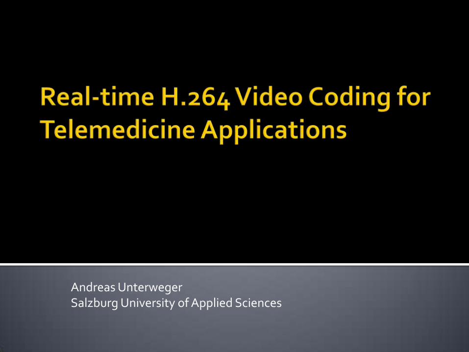
Two-dimensional extension of 1D DCT Spatial frequencies in gray images: change of
gray (signal) value per pixel Basis images: Higher vertical frequencies
Higher horizontal frequencies Image source: http://en.wikipedia.org/wiki/File:Dctjpeg.png
2D DCT
Image source: http://www.comp.nus.edu.sg/~cs5248/l01/DCTdemo.html

Theoretically lossless (beware of floating point rounding errors!)
Decorrelates input signal simplifies compression
Human visual system merely perceives loss of high frequencies simplifies compression
JPEG‘s 2D DCT works on shifted input data (8 bit values are shifted to a [-128;127] range)

Original
1 DCT coefficient (all others zero)
6 DCT coefficients (all others zero)
19 DCT coefficients (all others zero)
Image source: Matlab DCT demo

Reduce number of possible values instead of eliminating coefficients in transform domain
Division by factor, followed by rounding less bits required for representation
Quantization matrix Q specifies division factors for every coefficient higher quantization factors for higher frequencies
Image source: http://en.wikipedia.org/wiki/Jpeg

Quantization with Q
Image source: http://en.wikipedia.org/wiki/Jpeg

Quality in per cent (%) from 0 to 100 with according predefined quantization matrices
Custom quantization matrices possible Separate quantization matrices for luma and
chroma (higher quantizers for chroma) Be aware: 100% quality is not lossless
(quantization matrix for 100% quality contains many 1 values, but not only!)

Quality 100%
Quality 25%
Quality 50%
Quality 0%
Image source: http://www.fh-salzburg.ac.at
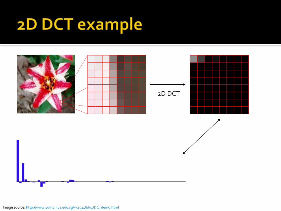
Subsequent zeros can be compressed more efficiently scan matrix in an order which makes subsequent zeros more likely
Higher frequencies are likely to be zeroed by quantization
Zigzag scan reorders
coefficients from low
to high frequencies
Image source: http://3.bp.blogspot.com/_6kpJik-Ua70/RkIT7NZCL_I/AAAAAAAAADE/acWC3QN2L24/s320/fig1.22.JPG

−26 −3 0 −3 −2 −6 2 −4 1 −3 1 1 5 1 2 −1 1 −1 2 0 0 0 0 0 −1 −1 0 0 0 0 0 0 0 0 0 0 0 0 0 0 0 0 0 0 0 0 0 0 0 0 0 0 0 0 0 0 0 0 0 0 0 0 0 0
Image sources: http://3.bp.blogspot.com/_6kpJik-Ua70/RkIT7NZCL_I/AAAAAAAAADE/acWC3QN2L24/s320/fig1.22.JPG; http://en.wikipedia.org/wiki/Jpeg

Lossless coding of coefficients scanned in zigzag order
Run-length encoding (RLE) for sequences of zeros with special „EOB“ marker at the end to indicate that the rest of the coefficients is zero
Huffman coding for actual coefficient differences based on their probability
Custom Huffman tables possible
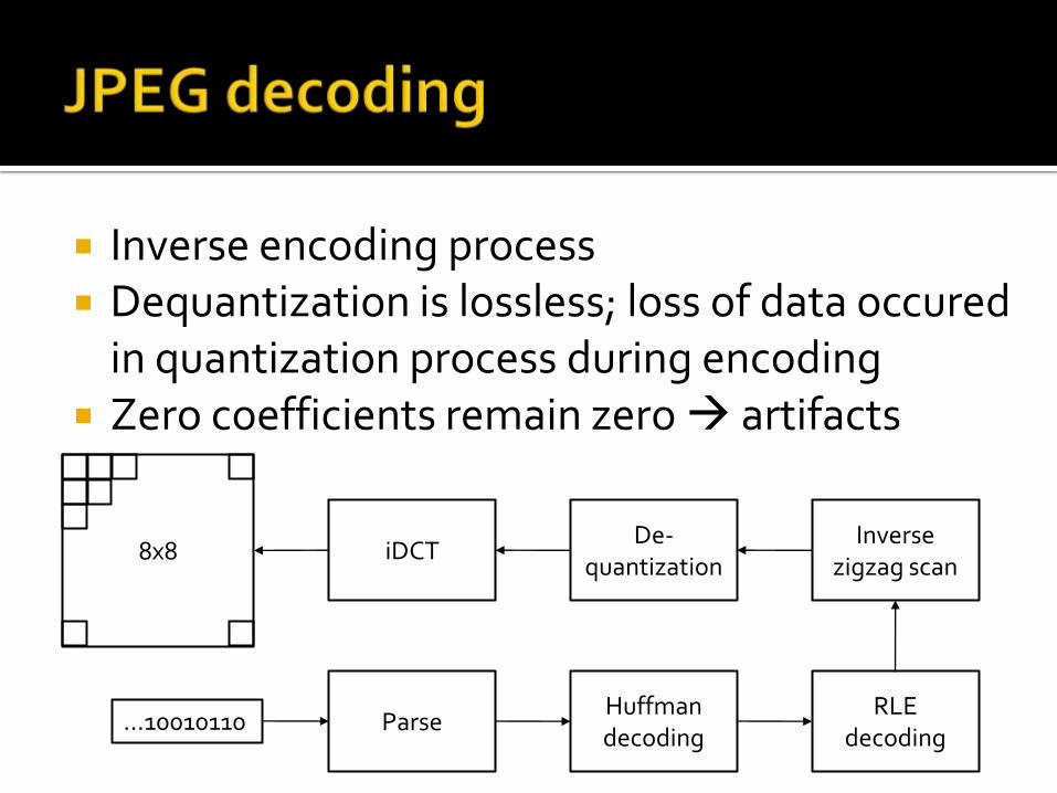
Inverse encoding process Dequantization is lossless; loss of data occured
in quantization process during encoding Zero coefficients remain zero artifacts
iDCT 8x8 De-
quantization Inverse
zigzag scan
RLE decoding
Huffman decoding
Parse …10010110

Blocking (macroblocks are encoded separately edges don‘t fit together smoothly)
Blurring (loss of too many high frequencies)
Blocking Blurring
Image sources: http://en.wikipedia.org/wiki/File:Lenna.png; http://www.fh-salzburg.ac.at

Ringing (edges cannot be accurately represented by „continuous“ base functions)
Over- and undershooting („minus“ red is cyan)
Image sources: http://en.wikipedia.org/wiki/File:Asterisk_with_jpg-artefacts.png; Punchihewa, G. A. D., Bailey, D. G., and Hogson, R. M.: Objective Evaluation of Edge Blur and Ringing Artefacts: Application to JPEG and JPEG 2000 Image Codecs. In Proceedings of Image and Vision Computing New Zealand 2005, pages 61-66, Dunedin, New Zealand, 2005

Basis function artifacts (very high quantization makes single basis functions visible)
Stair case artifacts (diagonal edges cannot be represented accurately by horizontal and vertical base functions)

Videos („motion pictures“) are sequences of images with high temporal correlation
Video coding uses image coding techniques and makes use of this temporal correlation
Motion is perceived at ca. 20 pictures per second, fluid perception requires a higher frame rate (depends on content, individual, and lightning conditions)
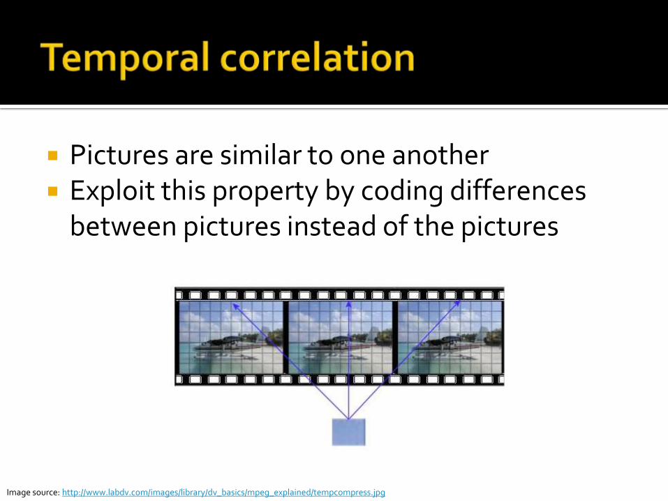
Pictures are similar to one another Exploit this property by coding differences
between pictures instead of the pictures
Image source: http://www.labdv.com/images/library/dv_basics/mpeg_explained/tempcompress.jpg

Pictures (frames) can be of different types
I (Intra) pictures/frames: Fully coded similar to JPEG algorithms described earlier (“key“ frames, relevant for scene changes and fast forwarding)
P (Predicted) pictures/frames: Only differences to previous pictures/frames are coded (use of temporal correlation between pictures)
More picture types to be described later

Used in P pictures to find similar macroblocks in previously coded pictures
Motion estimation: find best match
Image source: http://www-sipl.technion.ac.il/UploadedFiles/BlockBasedMotionEstimation.jpg

Motion vector: offset of matched macroblock Reference frame: macroblock match location Search window: area for match search
Image source: http://www.axis.com/products/video/about_networkvideo/img/7_1c.jpg

Calculate difference between macroblock match and current macroblock
Difference is treated like a regular macroblock (transform, quantization etc.)
To be saved additionally: reference frame and motion vector
Reconstruction by applying difference to reference macroblock in decoder

MPEG Standards
Joint ITU-T/MPEG
Standards
ITU-T Standards
H.261
1984 1994 1998 2000 2002 2004 1988 1990 1992 1986
H.264
H.263 H.263+ H.263++
MPEG-1 MPEG-2 MPEG-4
H.262/MPEG-2
1996

Image source: http://blog.toggle.com/free-programs-to-decompress-and-compress-files-2/

Specifies syntax and decoder only
Encoder design can be arbitrary as long as the syntax of the generated bit stream is valid
No guarantee for a specific quality as encoder decisions are not specified
Pre-Processing Encoding
Post-Processing / Error Recovery
Decoding
Input video
Output video
Scope of Standard
Image source: Kwon, S., Tamhankar, A. and Rao, K.R. Overview of H.264 / MPEG-4 Part10. http://www.powershow.com/view/19bc9-NDQyM/Overview_of_H_264_MPEG4_Part10_powerpoint_ppt_presentation (14.10.2010), 2004.

Image source: Unknown. Please contact me if you know the source

Image source: http://www2.engr.arizona.edu/~yangsong/layer.png

Image source: Wiegand, T. and Sullivan, G. J.: The H.264 | MPEG-4 AVC Video Coding Standard. http://ip.hhi.de/imagecom_G1/assets/pdfs/H264_03.pdf (14.10.2010), 2004

Video Coding Layer (VCL)
Picture partitioning
Motion-compensated prediction / Intra prediction
Predictive residual coding
Deblocking filter
Encoder test model
Network Abstraction Layer (NAL)
NAL units and types
RTP carriage and byte stream format (annex B)

Network-friendly representation New and simple syntax (not compatible with
previous standards like MPEG-2 Video)

Image source: http://digilib.ittelkom.ac.id/images/stories/artkel2/19/Struktur%20video%20H264AVC.JPG
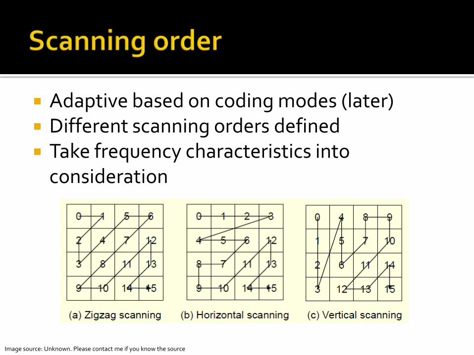
Adaptive based on coding modes (later) Different scanning orders defined Take frequency characteristics into
consideration
Image source: Unknown. Please contact me if you know the source

Image source: Jain, A. Introduction to H.264 Video Standard. http://www.powershow.com/view/ce503-OTc3M/Introduction_to_H264_Video_Standard_powerpoint_ppt_presentation (14.10.2011), 2011.

Integer transform to avoid floating point rounding errors and allow fast implementation
Derived from DCT with small differences 4x4 transform size for macroblock partitions
(later), macroblocks are of size 16x16
Image source: Wiegand, T., Sullivan, G. J., Bjontegaard, G. and Luthra, A.: Overview of the H.264/AVC Video Coding Standard, IEEE Transactions on Circuits and Systems for Video Technology, vol. 13, no. 7, pp. 560-576, July 2003

Image source: Unknown. Please contact me if you know the source
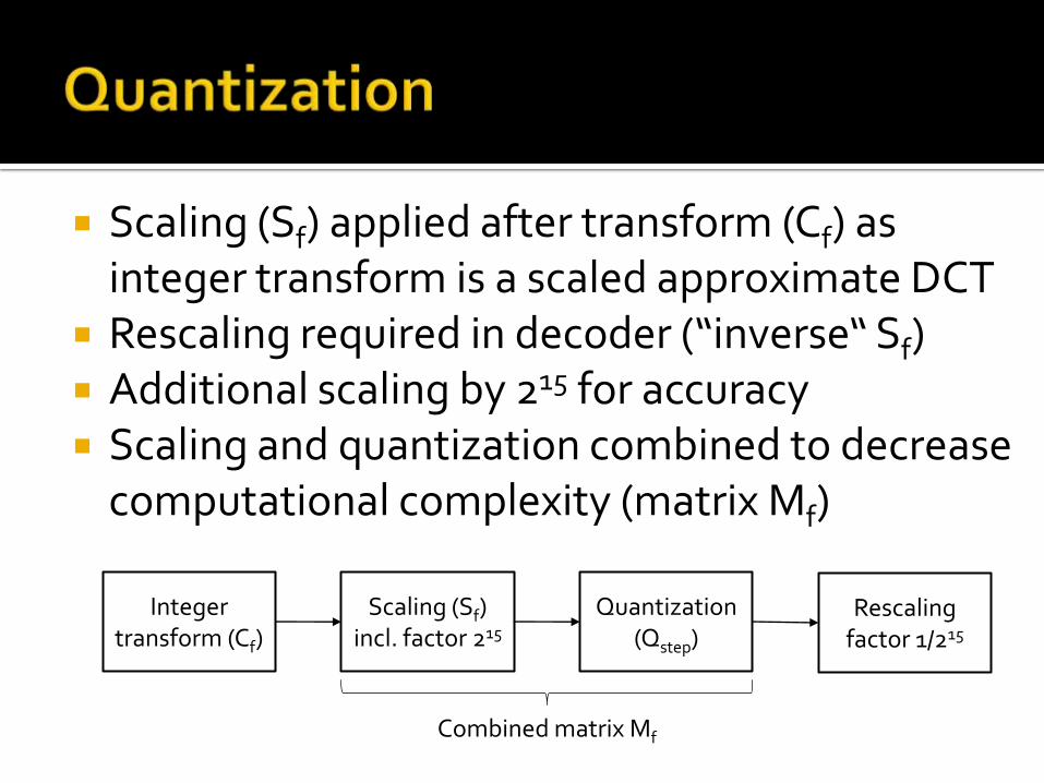
Scaling (Sf) applied after transform (Cf) as integer transform is a scaled approximate DCT
Rescaling required in decoder (“inverse“ Sf) Additional scaling by 215 for accuracy
Scaling and quantization combined to decrease computational complexity (matrix Mf)
Integer transform (Cf)
Scaling (Sf) incl. factor 215
Quantization (Qstep)
Rescaling factor 1/215
Combined matrix Mf

Quantization defined by quantization step value (Qstep) for input/output coefficients X/Y:
Left formula not explicitly defined in standard, only the combined matrix values Mfij
(Qstep) Implicit mij designed to consider human visual
perception (high frequency weighting like JPEG)
)(
215
stepij
ijf
ijijQm
SXroundY )( stepfijij QMXY
ij

Usually, a quantization parameter QP is used Qstep can be derived from QP Qstep value ratio is 21/6
QP doubles every 6 values of Qstep QP range is [0,51]
0 is quasi-lossless quantization
51 quantizes nearly all values to zero
Separate QP for every macroblock
Image source: Richardson, I. E. G.: H.264 / MPEG-4 Part 10: Transform & Quantization. http://www.vcodex.com/h264.html (18.1.2008), 2003.
Intra coded macroblocks are not fully coded, but predicted from their neighbours (use of spatial correlation within picture)
Either 4x4 or 16x16 block prediction possible Blocks at picture borders are also predicted Intra coded macroblocks can also appear in P
pictures if no appropriate match is found during motion estimation
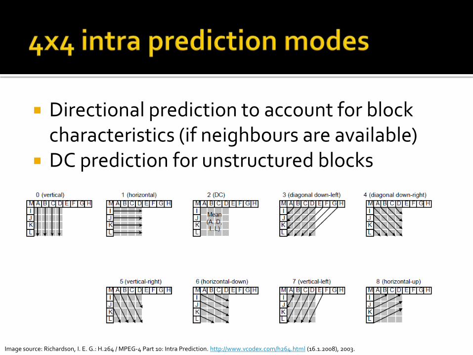
Directional prediction to account for block characteristics (if neighbours are available)
DC prediction for unstructured blocks
Image source: Richardson, I. E. G.: H.264 / MPEG-4 Part 10: Intra Prediction. http://www.vcodex.com/h264.html (16.1.2008), 2003.

Image source: Richardson, I. E. G.: H.264 / MPEG-4 Part 10: Intra Prediction. http://www.vcodex.com/h264.html (16.1.2008), 2003.

Best for homogenous picture regions Encoder can choose between single 16x16 intra
prediction or 16 separate 4x4 predictions Less signalling bits for 16x16 modes required
Image source: Richardson, I. E. G.: H.264 / MPEG-4 Part 10: Intra Prediction. http://www.vcodex.com/h264.html (16.1.2008), 2003.

Image source: Richardson, I. E. G.: H.264 / MPEG-4 Part 10: Intra Prediction. http://www.vcodex.com/h264.html (16.1.2008), 2003.

Only 4 chroma modes: vertical, horizontal, DC and planar
Both 8x8 chroma blocks (Cb and Cr, assuming 4:2:0 subsampling) in one macroblock use the same mode
Chroma modes can differ from luma modes Encoders can base chroma mode decision on
luma mode (slightly less accurate, but faster)

Prediction vs. final picture
16x16 modes in helmet area, rest: 4x4 modes
Image source: Richardson, I. E. G.: H.264 / MPEG-4 Part 10: Intra Prediction. http://www.vcodex.com/h264.html (16.1.2008), 2003.

Bidirectional prediction also allows prediction based on “future“ frames
Allow references to past or to “future“ pictures, depending on what costs less bits
Coding order has to be adapted as real “future“ prediction is not possible
Coding order and display order differ if B pictures are used

H.264 allows coding order to differ arbitrarily from display order
Coding order: 1 3 4 2 6 7 5 Display order: 1 2 3 4 5 6 7
Image source: http://focus.ti.com.cn/cn/graphics/shared/contributed_articles/video_compression_tradeoff_3.gif

References to B pictures allowed by H.264 References have to be coded first
Red: I or P, blue: B (first level), green: B (second level), yellow: B (third level)
Image source: http://ip.hhi.de/imagecom_G1/savce/images/fig_5.jpg

Processed frames are decoded and stored in the decoded picture buffer (DPB) for reference
The DPB size is usually constant within one video stream (max. 16)
DPB acts like a FIFO queue of pictures in coding order (simplified)
DPB can be cleared by special commands (memory management commands, MMCOs)

DPB is represented in form of two lists in the encoder: L0 and L1
L0 stores previously coded pictures in decreasing display order for P pictures
L1 is only used with B pictures Sophisticated ordering of lists according to
display order to use as few bits as possible to encode the index of the most likely reference

Possibility to mark reference pictures in either list as “long term“ (static)
Possibility to remove pictures by marking them as “unused for reference“
Arbitrary reordering operations possible on both lists through MMCOs
Simplified view in this presentation

Assumptions: DPB size 3, IPPP Picture numbers … 0, 1, 2, 3, 4 …
L0 after picture 0: 0 L0 after picture 1: 1 0 L0 after picture 2: 2 1 0 L0 after picture 3: 3 2 1 (0 drops!) L0 after picture 4: 4 3 2

“Instantaneous Decoding Refresh“ Coded like I pictures, but in special NAL unit Difference to I pictures: prediction border (no
references allowed to frames before IDR) Reference lists are cleared by IDR pictures Used as resynchronisation points (fast
forward)
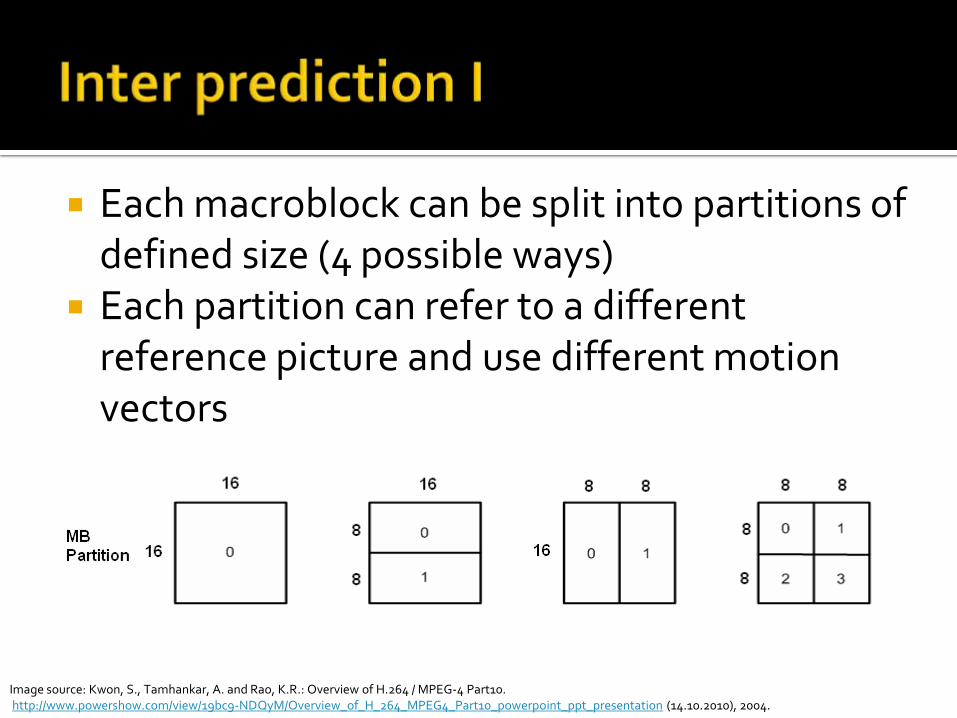
Each macroblock can be split into partitions of defined size (4 possible ways)
Each partition can refer to a different reference picture and use different motion vectors
Image source: Kwon, S., Tamhankar, A. and Rao, K.R.: Overview of H.264 / MPEG-4 Part10. http://www.powershow.com/view/19bc9-NDQyM/Overview_of_H_264_MPEG4_Part10_powerpoint_ppt_presentation (14.10.2010), 2004.

Each 8x8 partition can be further divided into sub partitions (4 possible ways)
Each sub partition within one partition must refer to the same reference picture, but can use different motion vectors
Image source: Kwon, S., Tamhankar, A. and Rao, K.R.: Overview of H.264 / MPEG-4 Part10. http://www.powershow.com/view/19bc9-NDQyM/Overview_of_H_264_MPEG4_Part10_powerpoint_ppt_presentation (14.10.2010), 2004.

Find best match in one of the reference frames Define region of NxN samples around the
current macroblock Search at all possible positions within this
region, calculating the SSD or MSE (later) between the current block and the match for each position
Choose the match with the smallest SSD/MSE Compute the motion vector from the position

Full (brute force) search is very time consuming and ineffective to find the absolute minimum
Various faster search strategies used in practice (diamond search, hexagonal search, three step search and many more)
Full search finds the absolute minimum, faster strategies may miss it or find a local minimum
Simple example: three step search (logarithmic)

Image source: http://commons.wikimedia.org/wiki/File:Three_step_search.PNG

Motion vector of current inter coded macroblock is derived from its neighbours‘ motion vectors or the last pictures‘ co-located macroblock (coding only the difference saves bits)
Direct mode: use derived motion vector (no motion vector difference), code residual
Skip mode: use derived motion vector and assume that there is no residual (1 bit only!)

Errors at macroblock borders propagate Prediction may be wrong (best match may be mathematically optimal, but not belong to the same object)

Inter block coding: Transform and quantize difference to reference block
On decoder side: use reference block referred to by motion vector and apply difference (inverse quantization and transform first)
Picture and/or object movement is described by motion vector and does not have to be coded (motion compensation)

P pictures: motion estimation on all (or N) pictures in the reference list (L0)
B pictures: bidirectional prediction from one picture of each reference list (L0 and L1): weighted sum (50:50) of both references
Bidirectional prediction can refer to two pictures which are actually the same picture (a picture can appear in both L0 and L1)
Bidirectional prediction around scene cuts

Weighted references‘ sums form prediction
Image source: Wiegand, T. and Sullivan, G. J.: The H.264 | MPEG-4 AVC Video Coding Standard. http://ip.hhi.de/imagecom_G1/assets/pdfs/H264_03.pdf (14.10.2010), 2004
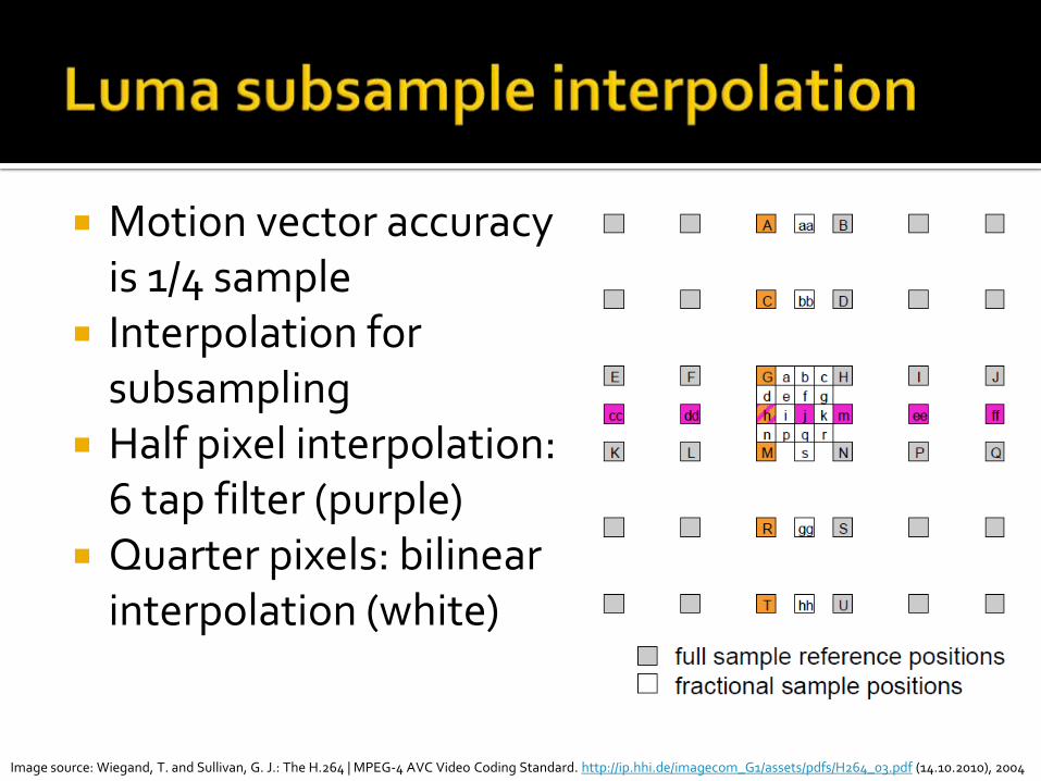
Motion vector accuracy is 1/4 sample Interpolation for subsampling Half pixel interpolation: 6 tap filter (purple) Quarter pixels: bilinear interpolation (white)
Image source: Wiegand, T. and Sullivan, G. J.: The H.264 | MPEG-4 AVC Video Coding Standard. http://ip.hhi.de/imagecom_G1/assets/pdfs/H264_03.pdf (14.10.2010), 2004

For 4:2:0 subsampling, chroma subsampling has to be accurate to 1/8 sample
Additional equation for all fractional chroma samples (subsamples) – details omitted here
Image source: Wiegand, T. and Sullivan, G. J.: The H.264 | MPEG-4 AVC Video Coding Standard. http://ip.hhi.de/imagecom_G1/assets/pdfs/H264_03.pdf (14.10.2010), 2004

Separation of picture into separate independent parts (slices)
No prediction between slices allowed parallelization possible
Deblocking at slice borders after coding Slice types within a picture can differ (I, P, B) Slices can be grouped into slice groups

Image source: Wiegand, T. and Sullivan, G. J.: The H.264 | MPEG-4 AVC Video Coding Standard. http://ip.hhi.de/imagecom_G1/assets/pdfs/H264_03.pdf (14.10.2010), 2004

In-loop deblocking filter specified by standard Deblocking applied after decoding (inverse
quantization) to each 4x4 block Reference pictures are stored deblocked Avoid blocking artifacts by edge blurring to
increase the perceived picture quality Preserve edges by using an adaptive threshold

Consideration of a variable amount of neighbouring samples, depending on edge strength
Sophisticated set of rules
Block coding modes (intra/inter)
Block border is a macroblock border?
Inter only: motion vector value differences
Inter only: equality of reference pictures
Etc.

Deblocking filter can be disabled (subjective decrease in picture quality, but faster encoding and decoding possible)
Thresholds can be adjusted and signalled through syntax elements specified by the H.264 standard
Change of thresholds changes behaviour of loop filter (stronger/weaker filtering)

Before deblocking After deblocking

Before deblocking After deblocking

Two codes: CAVLC and CABAC CAVLC (context-adaptive variable length
coding)
Optimized for compressing zeros in zig zag scanned 4x4 block coefficients (similar to JPEG)
CABAC (context-based adaptive binary arithmetic coding)
Coding tables depend on context (intra modes etc.)
10-20% more efficient than CAVLC, but also “slower“
Entropy coding is out of scope of presentation

Arbitrary slice order
Flexible macroblock order
Redundant slice
B slice
I slice
P slice
CAVLC
Weighted prediction
CABAC
Data partition
SI slice
SP slice
Extended Profile
Main Profile
Baseline Profile
Image source: Jain, A.: Introduction to H.264 Video Standard. http://www.powershow.com/view/ce503-OTc3M/Introduction_to_H264_Video_Standard_powerpoint_ppt_presentation (14.10.2011), 2011.

Limit resolution (number of macroblocks), decoding memory consumption, bit rate etc.
Device-specific level support (most set-top boxes p.e. support up to level 4.1)
Examples:
Level 1: QCIF 176x144@15fps
Level 3: SDTV 720x576@25fps
Level 4.1: HDTV 1920x1080@30fps
Level 5.1: Cinema 4096x2048@30fps (max. level)

Variable transform size (4x4 or 8x8) Support for higher bit rates and resolutions Support for actual lossless coding 4:4:4 and actual RGB support Support for more than 8 bits per sample (max.
12) for high fidelity applications (editing etc.) Custom quantization matrices

Large number of commercial encoders and decoders, few free implementations
Both encoder and decoder are very complex Decoders are equal in quality (at least in
theory) as the standard defines how decoding has to be done decoder speed matters
Encoder quality and feature implementations vary as the encoder design can be arbitrary

Decoders
ffmpeg (open source)
CoreCodec CoreAVC (commercial)
Encoders
x264 (open source)
Codecs (encoders and decoders combined)
MainConcept (commercial)
DivX H.264 (free and commerical version available)
Nero Digital (commercial)

Picture source: http://en.wikipedia.org/wiki/H.264/MPEG-4_AVC#Software_encoder_feature_comparison

Annex G of H.264 standard (amendment) Multiple video layers for different devices and
use cases, combined in a scalable manner Every device decodes m of n available layers,
according to ist capabilities and settings Compatible with regular H.264 decoders as
the base layer is a “normal“ H.264 bit stream (decode base layer only from SVC stream)

Temporal (picture rate, fps): the enhancement layers contain more pictures per second (usually in form of B pictures)
Spatial (picture size): the enhancement layers contain pictures with a higher resolution
SNR (picture quality): the enhancement layers contain pictures with a lower QP/higher quality
Arbitrary combination of dimensions possible

Image source: Unknown. Please contact me if you know the source

Recall: B pictures (hierarchical usage) Each B picture hierarchy level Tk is a temporal
scalability layer (k=0 for base layer) Optional bit stream elements to signal layers
Image source: Schwarz, H., Marpe, D. and Wiegand, T.: Overview of the Scalable Video Coding Extension of the H.264/AVC Standard. IEEE Transactions on Circuits and Systems for Video Technology, vol.17, no.9, pp.1103-1120, 2007

Enhancement layer is predicted from base layer (inter-layer intra/inter prediction)
Example: Combined temporal and spatial layers
Image source: Schwarz, H., Marpe, D. and Wiegand, T.: Overview of the Scalable Video Coding Extension of the H.264/AVC Standard. IEEE Transactions on Circuits and Systems for Video Technology, vol.17, no.9, pp.1103-1120, 2007

Upsampling from base layer also with arbitrary non-dyadic factors
Inter-layer intra prediction: base layer upsampling and residual coding (like intra)
Inter-layer inter prediction: motion vector and residual upsampling, coding of motion vector difference and upsampled residual (like inter)

Enhancement layers predict from base layer (prediction similar as for spatial scalability)
Only code residual to base layer data with a lower QP (higher quality)
Example: same resolution in enhancement layer, QP is decreased by about 20
Image source: Wiegand, T.: Scalable Video Coding in H.264/AVC. http://iphome.hhi.de/wiegand/assets/pdfs/DIC_SVC_07.pdf (14.10.2011), 2007

Image source: Schwarz, H., Marpe, D. and Wiegand, T.: Overview of the Scalable Video Coding Extension of the H.264/AVC Standard. IEEE Transactions on Circuits and Systems for Video Technology, vol.17, no.9, pp.1103-1120, 2007
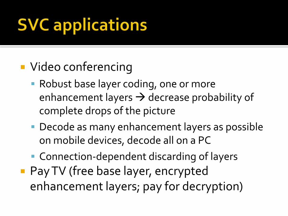
Video conferencing
Robust base layer coding, one or more enhancement layers decrease probability of complete drops of the picture
Decode as many enhancement layers as possible on mobile devices, decode all on a PC
Connection-dependent discarding of layers
Pay TV (free base layer, encrypted enhancement layers; pay for decryption)

Image source: Unknown. Please contact me if you know the source

Image source: Schwarz, H., Marpe, D. and Wiegand, D.: Overview of the Scalable H.264/MPEG4-AVC Extension, IEEE International Conference on Image Processing, 2006

No full SVC decoder for real-time applications currently available (November 2010)
Open source implementations support some basic decoding features (alpha state)
Only limited SVC encoders available (despite a reference implementation which cannot be used for real-time applications)
“H.265“ may include scalability

Annex H of H.264 standard (amendment) Coding of multiple views (p.e. two views for
stereoscopic 3D videos, like for 3D Blu-rays) Compatible with regular H.264 decoders (like
SVC) – only one view will be decoded Relatively small specification (syntax only) Prediction between views allows taking
advantage of picture correlation, reducing the overall bit rate (similar to SVC)

Image source: http://mpeg.chiariglione.org/sites/default/files/image004.jpg

Image source: Sun, H.: Multiview Video Coding. http://www.docstoc.com/docs/4749165/Multiview-Video-Coding-Huifang-Sun-and-Video-Team-Mitsubishi (14.10.2011), 2008

Virtual views can be interpolated from other views (example)
Interpolation quality depends on position of real “cameras“ Depth information is reconstructed as far as possible (hard)
Image source: Sun, H.: Multiview Video Coding. http://www.docstoc.com/docs/4749165/Multiview-Video-Coding-Huifang-Sun-and-Video-Team-Mitsubishi (14.10.2011), 2008

Image source: Sun, H.: Multiview Video Coding. http://www.docstoc.com/docs/4749165/Multiview-Video-Coding-Huifang-Sun-and-Video-Team-Mitsubishi (14.10.2011), 2008

Image source: Sun, H.: Multiview Video Coding. http://www.docstoc.com/docs/4749165/Multiview-Video-Coding-Huifang-Sun-and-Video-Team-Mitsubishi (14.10.2011), 2008

Image source: http://blog.toggle.com/free-programs-to-decompress-and-compress-files-2/

Video coding concept of real-time is different than in classical real-time systems with soft or hard deadlines
Frame (processing) rate of encoder has to be greater than or equal to frame rate of video in time average (in theory!)
Delay issues have to be coped with separately

Encoding speed is frame processing rate of encoder only (also depends on input)
Delay includes queues and more (ambiguous)
Encoder Frame n Input queue Output queue
Frame n
Scope of encoding speed
Scope of delay

Multiple definitions
Encoding delay (duration of pure frame encoding)
Encoder delay (duration from frame input to output by encoder; greater than or equal to encoding delay – beware of reordering!)
End-to-end delay (duration between recording and display for live streams; should be minimal)
Definition of delay depends on application Telemedicine applications require low delay

Camera processing delay
Camera-to-encoder transmission delay
Encoder delay Packaging and
transmission delay
Decoder delay Display delay
Image sources: Unknown. Please contact me if you know the source; http://www.popjolly.com/wp-content/uploads/2010/04/surgeons-300x194.jpg

Example: 25 fps recording (40ms per frame) Average recording delay for one frame: 20ms Average encoder delay also ca. 20ms (jitter) Transmission depends on channel and buffers:
>40ms (longer for TCP/IP and similar channels) Decoder has to decode whole picture: average
delay of 20ms (jitter due to different frames) 50 Hz display adds another min. 10ms delay

Total delay depends on various sources At 25fps, the minimum delay is at least
100ms (nearly 3 whole frames) Frame rate has significant impact (increasing
the frame rate lowers the delay) Some sources of delay cannot be minimized Some can, but require additional efforts
(extra hardware/software/money etc.)

Lower delay of each delay source Focus on main sources of delay
Transmission (faster connections, prioritized package handling etc.)
Encoding (faster encoder, different parameters)
Decoding complexity is influenced by encoder and its parameters (“ultra low delay“ (ULD) encoders/decoders help)
Transmission delay is a network layer issue

Video coding is always a trade-off between quality and bit rate
Quality is “inverse“ distortion Quality goal: best quality at given bit rate Bit rate goal: lowest bit rat at given quality Rate distortion optimization: achieve goals Base encoder decisions on RDO

Max. rate/min. distortion (source entropy)
Min. rate/max. distortion
Working point
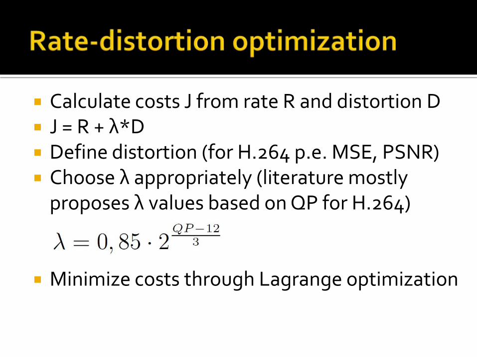
Calculate costs J from rate R and distortion D J = R + λ*D Define distortion (for H.264 p.e. MSE, PSNR) Choose λ appropriately (literature mostly
proposes λ values based on QP for H.264)
Minimize costs through Lagrange optimization

Example: intra prediction Encode one 4x4 block with all possible modes
and determine rates and distortions Calculate costs from rates and distortions Choose mode with lowest costs (optimization) Advantage: improves decisions, but only locally Disadvantage: expensive (coding time) Consider costs for error resilience decisions

Source: Unknown. Please contact me if you know the source

Resolution, chroma subsampling and complexity of input video (affects time)
Variable block size increases the number of inter modes to test (affects time)
RDO increases the number of total modes to test (affects time)
B pictures require picture reordering (affects delay); combined with RDO there are yet more modes to test (affects time)

Number of reference pictures for motion estimation prolongs search (affects time)
Search range for motion estimation prolongs search (affects time)
Adaptive loop deblocking filter requires additional time if not turned off (affects time)
CABAC is computationally more expensive than CAVLC (affects time)

x264 (open source H.264 encoder) uses presets to specify coding speed vs. compression efficiency trade-off
--preset parameter allows “ultrafast“ to “veryslow“ (and even “placebo“)
Default settings: 3 B pictures, 3 references (maximum DPB size), ME range 16, partitions: I 8x8 (high profile), I 4x4, P 16x8, P 8x16, P 8x8, P 8x4, P 4x8, P 4x4, B 16x8, B 8x16, B 8x8

“ultrafast“ parameter changes:
No 8x8 transform (high profile)
No B pictures
1 reference (maximum DPB size)
No mixed references with inter macroblocks
No CABAC
No deblocking
Full pixel diamond motion estimation

“veryslow“ parameter changes: 8 B pictures with adaptive B picture decision
16 references (maximum DPB size)
ME range 24
All partitions available
RDO for all modes and picture types
Psychovisual optimizations (p.e. Trellis quantization)
Psychovisual RDO

ultrafast veryfast faster fast medium slow slower veryslow placebo
fps 64,23 42,74 14,98 9,01 7,85 4,94 1,42 0,84 0,45
0
10
20
30
40
50
60
70
fps
Intel Core 2 Quad Q6600 720p encoding speed

Image source: CS MSU Graphics & Media Lab Video Group: MPEG-4 AVC/H.264 Video Codecs Comparison. http://compression.ru/video/codec_comparison/pdf/msu_mpeg_4_avc_h264_codec_comparison_2009.pdf (14.11.2010), 2009.

Image source: CS MSU Graphics & Media Lab Video Group: MPEG-4 AVC/H.264 Video Codecs Comparison. http://compression.ru/video/codec_comparison/pdf/msu_mpeg_4_avc_h264_codec_comparison_2009.pdf (14.11.2010), 2009.

Image source: http://blog.toggle.com/free-programs-to-decompress-and-compress-files-2/
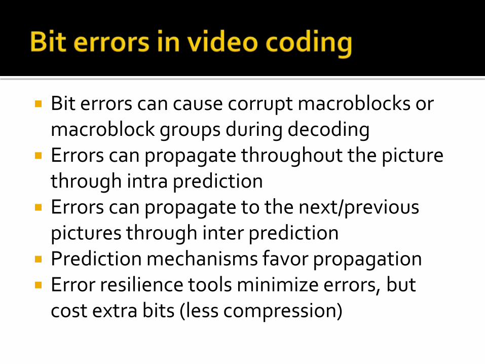
Bit errors can cause corrupt macroblocks or macroblock groups during decoding
Errors can propagate throughout the picture through intra prediction
Errors can propagate to the next/previous pictures through inter prediction
Prediction mechanisms favor propagation Error resilience tools minimize errors, but
cost extra bits (less compression)

Image source: Boulos, F., Wei Chen; Parrein, B.; Le Callet, P.: A new H.264/AVC error resilience model based on Regions of Interest. 17th International Packet Video Workshop, 2009, pp.1-9, 2009

Image source: Tsai, Y. C., Lin, C.-W. and Tsai, C.M.: H.264 error resilience coding based on multi-hypothesis motion-compensated prediction, Signal Processing: Image Communication, Vol.22, Issue 9, pp. 734-751, 2007

Extended profile specifies coding tools for error resilience
Some tools also available in baseline profile Parameter sets used to synchronize encoder
and decoder (resolutions, tools used etc.) SP/SI frames for stream switching are also
available, but not mentioned here Error concealment is not part of the standard

Slice data (encoded macroblocks) is split into three data partitions: A, B and C
Partition A: slice header and macroblock header information (coding mode etc.)
Partition B: macroblock data for intra blocks Partition C: macroblock data for inter blocks Each partition is encapsulated in a separate
NAL unit priorization of A over B/C possible

Possibility to code macroblocks more than one time and send them as additional, but redundant slice (lower quality possible)
Decoder favors primary slice and discards the redundant slice if both are available
If the primary slice is not available, the decoder uses the according redundant slice (if available) reconstruction possible
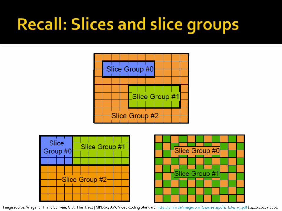
Image source: Wiegand, T. and Sullivan, G. J.: The H.264 | MPEG-4 AVC Video Coding Standard. http://ip.hhi.de/imagecom_G1/assets/pdfs/H264_03.pdf (14.10.2010), 2004
Defines fine-grain macroblock association with slice groups
Different scanning patterns possible Dispersing macroblocks reduces sensitivity to
burst noise on transmission channel Both implicit and explicit assignment to slice
groups possible through multiple map types
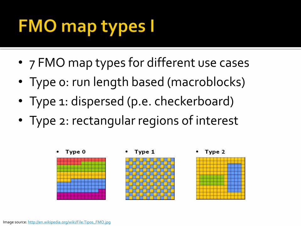
• 7 FMO map types for different use cases
• Type 0: run length based (macroblocks)
• Type 1: dispersed (p.e. checkerboard)
• Type 2: rectangular regions of interest
Image source: http://en.wikipedia.org/wiki/File:Tipos_FMO.jpg
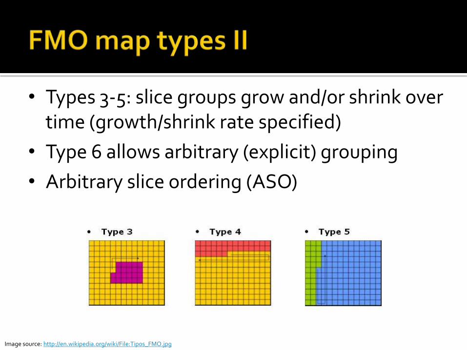
• Types 3-5: slice groups grow and/or shrink over time (growth/shrink rate specified)
• Type 6 allows arbitrary (explicit) grouping
• Arbitrary slice ordering (ASO)
Image source: http://en.wikipedia.org/wiki/File:Tipos_FMO.jpg

Slices don‘t have to be transmitted in scanning order (arbitrary ordering possible)
Reordering may reduce effect of burst noise as it does not effect subsequent picture regions
Priorization of slices or slice groups possible as every slice is contained in a separate NAL unit
Fine-grain macroblock association possible with flexible macroblock ordering (FMO)

Image source: Jain, A. Introduction to H.264 Video Standard. http://www.powershow.com/view/ce503-OTc3M/Introduction_to_H264_Video_Standard_powerpoint_ppt_presentation (14.10.2011), 2011.

Redundant slices require additional coding (affects time)
ASO is theoretically time-neutral as the number of coded blocks/slices stays the same
FMO may slow down the encoder due to cache misses due to dispersed macroblocks in slice groups (affects time)
Decoding complexity increases (affects time)

H.264 specifies that corrupt NAL units are to be discarded (syntax errors or semantical errors can be detected, some others cannot)
Error concealment may be applied to all areas where data is missing (optional)
Standard proposes concealment methods Different methods proposed by various
research groups

Syntax error detection
Illegal values of syntax elements
Illegal synchronisation/header (0x000001)
Coded macroblock data contains more elements than specified (p.e. more than 16 in a 4x4 block)
Illegal CAVLC/CABAC code (words)
Semantics error detection
Out of range luma or chroma values
Invalid states during decoding

Recall: data partitions A, B and C to prioritize information (A is the most important partition)
Recall: B/C contain intra/inter coded data
Image source: Kumar, S., Xu, L., Mandal, M. K. and Panchanathan, S.: Error Resiliency Schemes in H.264/AVC Standard. Elsevier Journal of Visual Communication & Image Representation (Special issue on Emerging H.264/AVC Video Coding Standard), Vol. 17(2), 2006

Image source: Kumar, S., Xu, L., Mandal, M. K. and Panchanathan, S.: Error Resiliency Schemes in H.264/AVC Standard. Elsevier Journal of Visual Communication & Image Representation (Special issue on Emerging H.264/AVC Video Coding Standard), Vol. 17(2), 2006

Image source: Kumar, S., Xu, L., Mandal, M. K. and Panchanathan, S.: Error Resiliency Schemes in H.264/AVC Standard. Elsevier Journal of Visual Communication & Image Representation (Special issue on Emerging H.264/AVC Video Coding Standard), Vol. 17(2), 2006

Original Decoded (err.) “Copy“ concealment
• Checkerboard pattern allows interpolation if one slice group gets lost or damaged
• Concealment: use previous pictures‘ blocks
Image source: Kolkeri, V. S., Koul, M. S., Lee, J. H. and Rao, K. R.: Error Concealment Techniques in H.264/AVC For Wireless Video Transmission In Mobile Networks. http://students.uta.edu/ms/msk3794/docs/ERROR_CONCEALMENT_TECHNIQUES-JAES2009.pdf (14.10.2011), 2008

Weighted pixel averaging from neighbouring macroblock samples
Neighbours have to be available If neighbours are also interpolated, prediction becomes worse
Image source: Kumar, S., Xu, L., Mandal, M. K. and Panchanathan, S.: Error Resiliency Schemes in H.264/AVC Standard. Elsevier Journal of Visual Communication & Image Representation (Special issue on Emerging H.264/AVC Video Coding Standard), Vol. 17(2), 2006
Motion vectors tend to correlate in small regions and over a small number of pictures
If motion vectors are lost, they may be predicted from the neighbouring blocks and/or the reference frame‘s co-located macroblocks
Motion vector prediction (based on median, average or similar techniques) often fails
In some cases: copy co-located reference block

Predict block from neighbouring DC coefficients (make use of spatial correlation)
Predict block in form of a weighted average of the available neighbouring blocks
Interpolate one sample from n neighbouring samples using linear, bilinear or any other form of interpolation to weigh the n pixels according to their distance

Based on scene cut detection to force zero motion vectors for lost blocks
Picture n-1 20% loss
Picture n 20% loss
Original Decoded (err.) Concealed Image source: Su, L., Zhang, Y., Gao, W., Huang, Q. and Lu, Y.: Improved error concealment algorithms based on H.264/AVC non-normative decoder. 2004 IEEE International Conference on Multimedia and Expo, vol.3, pp. 1671-1674, 2004

Dominant edge detection from neighbouring macroblocks for directional interpolation
Weighted averaging vs. edge detection
Image source: Nemethova, O., Al-Moghrabi, A. and Rupp, M.: Flexible Error Concealment for H.264 Based on Directional Interpolation. 2005 International Conference on Wireless Networks, Communications and Mobile Computing, vol.2, pp.1255-1260, 2005

Theoretical methods not for practical use Example: determine regions of interest (green
box) in the picture through subjective tests and force intra prediction for affected blocks
Image source: Boulos, F., Wei Chen; Parrein, B.; Le Callet, P.: A new H.264/AVC error resilience model based on Regions of Interest. 17th International Packet Video Workshop, 2009, pp.1-9, 2009

Different methods for objective and subjective quality measurement
Subjective measurement using humans who rate the video quality on a defined scale (costly and time consuming)
Objective measurement using mathematical formulas can only approximate subjective measurements but is less time consuming

Measure difference between original image/video and its encoded/decoded version
Sum of absolute differences (SAD) Sum of absolute total differences (SATD) Sum of squared differences (SSD) Mean squared error (MSE) (Y-)PSNR derived from MSE (logarithmic) More metrics

MSE for m times n samples for original samples I and coded samples K
Y-PSNR (luma only), MAXI=28-1 for 8 bit samples
PSNR calculation for color pictures
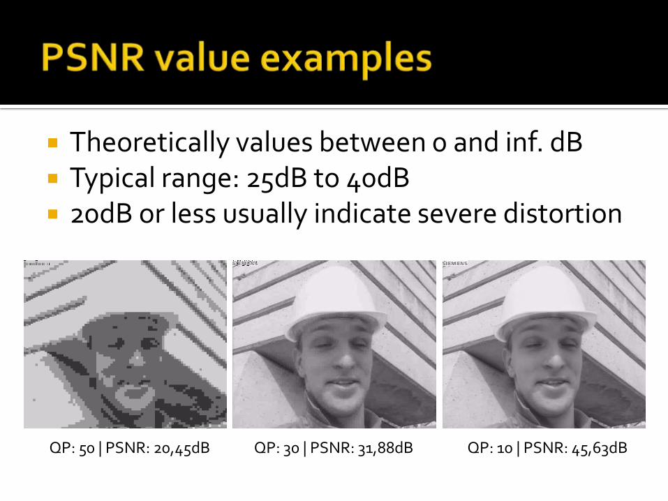
Theoretically values between 0 and inf. dB Typical range: 25dB to 40dB 20dB or less usually indicate severe distortion
QP: 50 | PSNR: 20,45dB QP: 10 | PSNR: 45,63dB QP: 30 | PSNR: 31,88dB

Both coded pictures have about the same MSE. Can you see why?
Image source: Nadenau, M.: Integration of Human Color Vision Models into High Quality Image Compression. PhD thesis, Ecole Polytechnique Federale de Lausanne, 2000

Approximate subjective quality measurement by measuring structual similarity of image blocks (typically 8x8 samples)
Take contrast, blurriness and other paramters into consideration (similar to human eye)
More complex to calculate than Y-PSNR, but also higher correlation with subjective quality measurements (typical trade-off)

Y-PSNR: 32,08dB SSIM: 0,865
Y-PSNR: 35,50dB SSIM: 0,921
Y-PSNR range: 0 to inf. dB (best) SSIM: -1 to 1 (best)
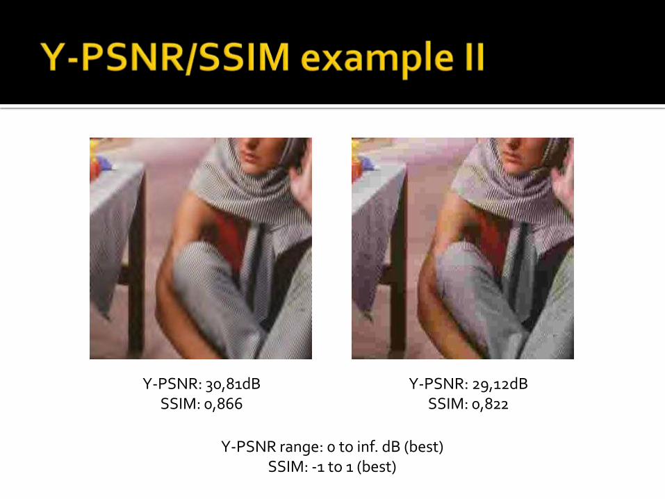
Y-PSNR: 30,81dB SSIM: 0,866
Y-PSNR: 29,12dB SSIM: 0,822
Y-PSNR range: 0 to inf. dB (best) SSIM: -1 to 1 (best)

Complete loss of macroblocks or whole slices is hard to measure (as effect on the picture(s))
Complete loss is nearly always noticeable, but concealment can hide it up to a certain extent
Y-PSNR and SSIM make sense in error concealed pictures, but not in lost ones
Measuring quality of pictures with completely lost macroblocks or slices is difficult

Practical example of error resilience effects (increase in bit rate, increase in encoding time)
Practical example of error concealment effects (loss prevention, method comparison)
Error resilience and concealment demo
NAL simulator with virtual, error prone transmission channel
Extended version of x264 with error resilience tools
Extended version of ffmpeg with error concealment

Image source: http://blog.toggle.com/free-programs-to-decompress-and-compress-files-2/
Standardization is currently taking place Code name HEVC (high efficiency video
coding), final name possibly H.264+ or H.265 or even HEVC (not decided yet)
Goal: same quality at half the bit rate of H.264 Planned: incorporates SVC and MVC Planned: compatible with H.264 syntax Proposals for new or refined coding tools

Massive parallelization
Parallelized entropy coding (hardly parallelizable in H.264) for both CABAC and CAVLC
„Slicing“ concepts for entropy coding
Increased macroblock size
32x32 or even 64x64 macroblocks
Arbitrary rectangular partitions (adaptive borders)
Increased transform size (16x16 or 32x32 DCT)

Advanced loop and interpolation filtering
Integrated noise filtering (p.e. Wiener filter)
1/8 or 1/12 pixel motion estimation
Multiple loop filters
Various new ideas
Non-rectangular motion partition shapes
„Superblocks“ consisting of multiple macroblocks
New entropy coding algorithms

Proposals have been evaluated in April 2010 Test model has been selected in October 2010 July 2012: Final standard approval (planned)
H.264 adoption took several years
Hardware requirements (standard completed 2003)
Codec development (hardware and software)
Broad support (players, GPU acceleration etc.)
Incorporation in other standards (DVB, Blu-ray etc.)

Questions?