1  

 

Beyond power calculations: Assessing Type S (sign) and Type M (magnitude) errors1

Andrew Gelman2 and John Carlin3

Abstract. Statistical power analysis provides the conventional approach to assess error

rates when designing a research study. But power analysis is flawed in that it places a

narrow emphasis on statistical significance as the primary focus of study design. In

noisy, small-sample settings, statistically significant results can often be misleading. To

help researchers address this problem in the context of their own studies, we recommend

design calculations that estimate (i) the probability of an estimate being in the wrong

direction (“Type S error”) and (ii) the factor by which the magnitude of an effect might

be overestimated (“Type M error” or exaggeration ratio). We illustrate with examples

from recent published research and discuss the largest challenge in a design calculation:

coming up with reasonable estimates of plausible effect sizes based on external

information.

Keywords: design calculation, exaggeration ratio, power analysis, replication crisis,

statistical significance, Type M error, Type S error

                                                                                                                         1 For Perspectives on Psychological Science. We thank Eric Loken, Deborah Mayo, Alison Ledgerwood, Barbara Spellman, and three reviewers for helpful comments and the Institute of Education Sciences, Department of Energy, National Science Foundation, and National Security Agency for partial support of this work. 2 Department of Statistics and Department of Political Science, Columbia University, New York, gelman@stat.columbia.edu, http://www.stat.columbia.edu/~gelman/ 3 Clinical Epidemiology and Biostatistics Unit, Murdoch Children’s Research Institute, Melbourne; Department of Paediatrics and School of Population & Global Health, University of Melbourne, Parkville, Victoria, Australia.

2  

 

Introduction

You’ve just finished running an experiment. You analyze the results, and you find a

significant effect. Success! But wait: how much information does your study really give you?

How much should you trust your results? In this paper, we show that when researchers use small

samples and noisy measurements to study small effects—as they often do in psychology, as well

as other disciplines—a significant result is often surprisingly likely to be in the wrong direction

and to greatly overestimate an effect.

In this paper we examine some critical issues related to power analysis and the interpretation

of findings arising from studies of small sample size. We highlight the use of external

information to inform estimates of true effect size and propose what we call a design analysis—a

set of statistical calculations about what could happen under hypothetical replications of a

study—that focuses on estimates and uncertainties rather than on statistical significance.

As a reminder, the power of a statistical test is the probability that it correctly rejects the null

hypothesis. For any experimental design, the power of a study depends on sample size,

measurement variance, the number of comparisons being performed, and the size of the effects

being studied. In general, the larger the effect, the higher the power; thus, power calculations are

performed conditional on some assumption of the size of the effect. Power calculations also

depend on other assumptions, most notably the size of measurement error, but these are typically

not so difficult to assess using available data.

It is of course not at all new to recommend the use of statistical calculations based on prior

guesses of effect sizes, to inform the design of studies. What is new about the present paper is:

1. We suggest that design calculations be performed after as well as before data collection

and analysis;

3  

 

2. We frame our calculations not in terms of Type 1 and Type 2 errors but rather type Type

S (sign) and type Type M (magnitude) errors, which relate to the probability that claims

with confidence have the wrong sign or are far in magnitude from underlying effect sizes.

Design calculations, whether prospective or retrospective, should be based on realistic external

estimates of effect sizes. This is not widely understood since it is common practice to using use

estimates from the current study’s data or from isolated reports in the literature, both of which

can overestimate the magnitude of effects.

The idea that published effect size estimates tend to be too large, essentially because of

publication bias, is not new (Lane and Dunlap, 1987, Hedges, 1984, and more recently, Button et

al., 2013). Here we provide a method to apply to particular studies, making use of information

specific to the problem at hand. We illustrate with recent published studies in biology and

psychology and conclude with a discussion of the broader implications of these ideas.

One practical implication of realistic design analysis is to suggest larger sample sizes than are

commonly used in psychology. We believe that researchers typically think of statistical power

as a tradeoff between the cost of performing a study (acutely felt in a medical context in which

lives can be at stake) and the potential benefit of making a scientific discovery (operationalized

as a statistically significant finding, ideally in the direction posited). The problem, though, is

that if sample size is too small, in relation to the true effect size, then what appears to be a win

(statistical significance) may really be a loss (in the form of a claim that does not replicate).

Conventional design or power calculations and the effect size assumption

The starting point of any design calculation is the postulated effect size because, of course, we

do not know the true effect size. We recommend thinking of the true effect as that which would

4  

 

be observed in a hypothetical infinitely large sample. This framing emphasizes that the

researcher needs to have a clear idea of the population of interest: the hypothetical study of very

large (effectively infinite) sample size should be imaginable in some sense.

How do researchers generally specify effect sizes for power calculations? As detailed in

numerous texts and articles, there are two standard approaches:

- Empirical: Assuming an effect size equal to the estimate from a previous study (if

performed prospectively, in which case the target sample size is generally specified such

that a desirable level of power is achieved) or from the data at hand (if performed

retrospectively); or

- Based on goals: Assuming an effect size deemed to be substantively important or more

specifically the minimum effect that would be substantively important (without a good

argument that such an effects are is likely to be true).

We suggest that each of the conventional approaches above is likely to lead either to performing

studies that are too small or to misinterpreting study findings after completion. Effect size

estimates based on preliminary data (either within the study or elsewhere) are likely to be

misleading because they are generally based on small samples, and when the preliminary results

appear interesting they are most likely biased towards unrealistically large effects (by a

combination of selection biases and the play of chance). Determining power under an effect size

considered to be of “minimal substantive importance” can also leads to specifying effect sizes

that are larger than what is likely to be the true effect.

Once data have been collected and a result is in hand, statistical authorities commonly

recommend against performing power calculations (see, for example, Goodman and Berlin,

1994, Senn, 2002, and Lenth, 2007). Hoenig and Heisey (2001) wrote, “Dismayingly, there is a

5  

 

large, current literature that advocates the inappropriate use of post-experiment power

calculations as a guide to interpreting tests with statistically nonsignificant results.” As these

authors have noted, there are two problems with retrospective power analysis as it is commonly

done: (1) effect size and thus power is generally overestimated, sometimes drastically so, when

computed based on statistically significant results; (2) from the other direction, post-hoc power

analysis often seems to be used as an alibi to explain away non-significant findings.

Although we agree with these critiques, we find retrospective design analysis to be useful and

we recommend it in particular when apparently strong (statistically significant) evidence for non-

null effects has been found. The key difference between our proposal and the usual retrospective

power calculations that are deplored in the statistical literature is, first, that we are focused on the

sign and direction of effects rather than on statistical significance; and, most importantly, that we

base our design analysis (whether prospective or retrospective) on an effect size that is

determined from literature review or other information external to the data at hand.

Our recommended approach to design analysis

Suppose you perform a study that yields an estimate d with standard error s. For concreteness

the reader may think of d as the estimate of the mean difference in a continuous outcome

measure between two treatment conditions, but the discussion applies to any estimate of a well-

defined population parameter. The standard procedure is to report the result as statistically

significant if p<.05 (which in many situations would correspond approximately to finding that

|d/s| > 2) and inconclusive (or as evidence in favor of the null hypothesis) otherwise.4

                                                                                                                         4  See Broer et al. (2013) for a recent empirical examination of the need for context-specific significance thresholds to deal with the problem of multiple comparisons.

6  

 

The next step is to consider a true effect size D (the value that d would take if observed in a

very large sample), hypothesized based on external information (other available data, literature

review, and modeling as appropriate to apply to the problem at hand). We then define the

random variable drep to be the estimate obtained from in a hypothetical future replicated study

also with underlying effect size D and standard error s.

Our analysis does not involve elaborate mathematical derivations but it does represent a

conceptual leap by introducing the hypothetical drep. This step is required so that we can make

general statements about the design of a study—the relation between the true effect size and

what can be learned from the data—without relying on a particular, possibly highly noisy, point

estimate.

We consider three key summaries based on the probability model for drep:

- The power: the probability that the replication drep is larger (in absolute value) than the

critical value that is considered to define “statistical significance” in this analysis.

- The Type S error rate: the probability that the replicated estimate has the incorrect sign,

if it is statistically significantly different from zero.

- The exaggeration ratio (expected Type M error): the expectation of the absolute value of

the estimate divided by the effect size, if statistically significantly different from zero.

We have implemented these calculations in an R function, retrodesign(). The inputs to the

function are D (the hypothesized true effect size), s (the standard error of the estimate), α (the

statistical significance threshold, e.g., 0.05), and df (the degrees of freedom). The function

returns three outputs: the power, the type S error rate, and the exaggeration ratio, all computed

7  

 

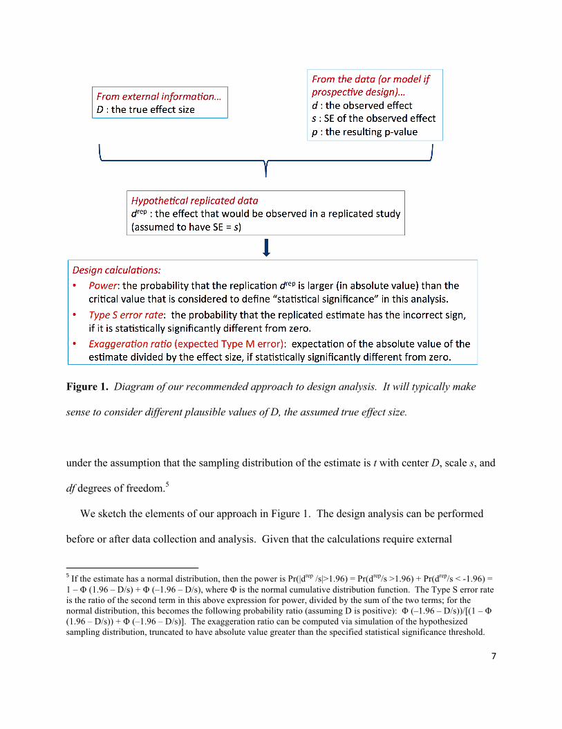
Figure 1. Diagram of our recommended approach to design analysis. It will typically make

sense to consider different plausible values of D, the assumed true effect size.

under the assumption that the sampling distribution of the estimate is t with center D, scale s, and

df degrees of freedom.5

We sketch the elements of our approach in Figure 1. The design analysis can be performed

before or after data collection and analysis. Given that the calculations require external

                                                                                                                         5  If the estimate has a normal distribution, then the power is Pr(|drep /s|>1.96) = Pr(drep/s >1.96) + Pr(drep/s < -1.96) = 1 – Φ (1.96 – D/s) + Φ (–1.96 – D/s), where Φ is the normal cumulative distribution function. The Type S error rate is the ratio of the second term in this above expression for power, divided by the sum of the two terms; for the normal distribution, this becomes the following probability ratio (assuming D is positive): Φ (–1.96 – D/s))/[(1 – Φ (1.96 – D/s)) + Φ (–1.96 – D/s)]. The exaggeration ratio can be computed via simulation of the hypothesized sampling distribution, truncated to have absolute value greater than the specified statistical significance threshold.

8  

 

information about effect size, one might ask why would a researcher ever do them after

conducting a study, when it is too late to do anything about potential problems? Our response is

twofold. First, it is indeed preferable to do a design analysis ahead of time, but a researcher can

analyze data in many different ways—indeed, an important part of data analysis is the discovery

of unanticipated patterns (Tukey, 1977) so that it is unreasonable to suppose that all potential

analyses could have been determined ahead of time. The second reason for performing post-data

design calculations is that they can be a useful way to interpret the results from a data analysis,

as we next demonstrate in two examples.

What is the relation between power, Type S error rate, and exaggeration ratio? We can work

this out for estimates that are unbiased and normally distributed, which can be a reasonable

approximation in many settings, including averages, differences, and linear regression.

It is standard in prospective studies in public health to require a power of 80%, that is, a

probability of 0.8 that the estimate will be statistically significant at the 95% level, under some

prior assumption about the effect size. Under the normal distribution, the power will be 80% if

the true effect is 2.8 standard errors away from zero. Running retrodesign()with D=2.8,

s=1, α=0.05, and df=infinity, we get power=0.80, a type S error rate of 1.2x10-6, and an expected

exaggeration factor of 1.12. Thus, if the power is this high, we have nothing to worry about

regarding the direction of any statistically significant estimate, and the overestimation of the

magnitude of the effect will be small.

However, studies in psychology typically do not have 80% power, for two reasons. First,

experiments in psychology are relatively inexpensive and are subject to fewer restrictions,

compared to medical experiments where funders typically require a minimum level of power

before approving a study. Second, formal power calculations are often optimistic, partly in

9  

 

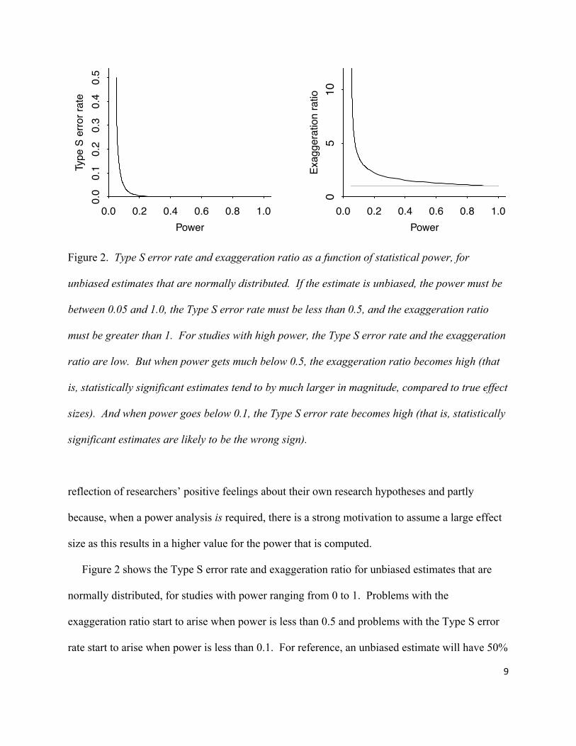
Figure 2. Type S error rate and exaggeration ratio as a function of statistical power, for

unbiased estimates that are normally distributed. If the estimate is unbiased, the power must be

between 0.05 and 1.0, the Type S error rate must be less than 0.5, and the exaggeration ratio

must be greater than 1. For studies with high power, the Type S error rate and the exaggeration

ratio are low. But when power gets much below 0.5, the exaggeration ratio becomes high (that

is, statistically significant estimates tend to by much larger in magnitude, compared to true effect

sizes). And when power goes below 0.1, the Type S error rate becomes high (that is, statistically

significant estimates are likely to be the wrong sign).

reflection of researchers’ positive feelings about their own research hypotheses and partly

because, when a power analysis is required, there is a strong motivation to assume a large effect

size as this results in a higher value for the power that is computed.

Figure 2 shows the Type S error rate and exaggeration ratio for unbiased estimates that are

normally distributed, for studies with power ranging from 0 to 1. Problems with the

exaggeration ratio start to arise when power is less than 0.5 and problems with the Type S error

rate start to arise when power is less than 0.1. For reference, an unbiased estimate will have 50%

0.0 0.2 0.4 0.6 0.8 1.0

0.0

0.1

0.2

0.3

0.4

0.5

Power

Type

S e

rror r

ate

0.0 0.2 0.4 0.6 0.8 1.0Power

Exag

gera

tion

ratio

05

10

10  

 

power if the true effect is 2 standard errors away from zero, it will have 17% power if the true

effect is 1 standard error away from 0, and it will have 10% power if the true effect is .65

standard errors away from 0. All these are possible in psychology experiments with small

samples, high variation (such as arises naturally in between-subject designs), and small effects.

Example: Beauty and sex ratios

We first developed the ideas in this paper in the context of a finding by Kanazawa (2007)

from a sample of 2972 respondents from the National Longitudinal Study of Adolescent Health.

This is not a small sample size by the standards of psychology but in this case the sizes of any

true effects are so small (as we shall discuss below) that a much larger sample would be required

to gather any useful information here.

Each of the people surveyed had been assigned an “attractiveness” rating on a 1-5 scale and

then, years later, had at least one child. 56% of the first-born children of the parents in the most

attractive category were girls, compared to 48% in the other groups. The author’s focus on this

particular comparison among the many others that might have been made may be questioned

(Gelman, 2007). For the purpose of illustration, however, we shall stick with the estimated

difference of 8 percentage points with p-value 0.015, hence statistically significant at the

conventional 5% level. Kanazawa (2007) followed the usual practice and just stopped right here,

claiming a novel finding.

We will go one step further, though, and perform a design analysis. We need to postulate an

effect size, which will not be 8 percentage points. Instead, we hypothesize a range of true effect

sizes using the scientific literature. From Gelman and Weakliem (2009):

11  

 

“There is a large literature on variation in the sex ratio of human births, and the effects

that have been found have been on the order of 1 percentage point (for example, the

probability of a girl birth shifting from 48.5 percent to 49.5 percent). Variation

attributable to factors such as race, parental age, birth order, maternal weight, partnership

status and season of birth is estimated at from less than 0.3 percentage points to about 2

percentage points, with larger changes (as high as 3 percentage points) arising under

economic conditions of poverty and famine. That extreme deprivation increases the

proportion of girl births is no surprise, given reliable findings that male fetuses (and also

male babies and adults) are more likely than females to die under adverse conditions.”

Given the generally small observed differences in sex ratios as well as the noisiness of the

subjective attractiveness rating used in this particular study, we expect any true differences in the

probability of girl birth to be well under 1 percentage point. It is standard for prospective design

analyses to be performed under a range of assumptions, and we shall do the same here,

hypothesizing effect sizes of 0.1, 0.3, and 1.0 percentage points. Under each hypothesis, we

consider what might happen in a study with sample size equal to that of Kanazawa (2007).

Again, we ignore multiple comparisons issues and take the published claim of statistical

significance at face value: from the reported estimate of 8% and p-value of 0.015, we can

deduce that the standard error of the difference was 3.3%. Such a result will be statistically

significant only if the estimate is at least 1.96 standard errors from zero; that is, the estimated

difference in proportion girls, comparing beautiful parents to others, would have to be more than

6.5 percentage points or less than –6.5.

The results of our proposed design calculations for this example are displayed in Table 1, for

three hypothesized true effect sizes. If the true difference of is 0.1% or –0.1% (probability of girl

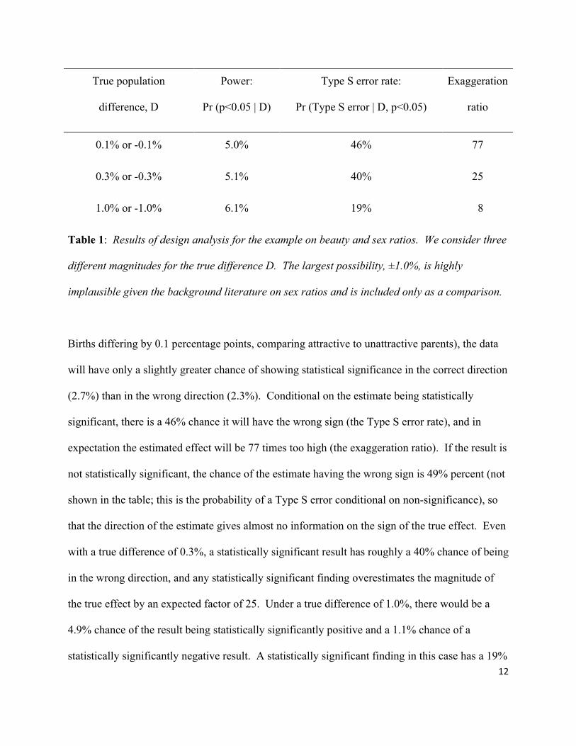
12  

 

True population

difference, D

Power:

Pr (p<0.05 | D)

Type S error rate:

Pr (Type S error | D, p<0.05)

Exaggeration

ratio

0.1% or -0.1% 5.0% 46% 77

0.3% or -0.3% 5.1% 40% 25

1.0% or -1.0% 6.1% 19% 8

Table 1: Results of design analysis for the example on beauty and sex ratios. We consider three

different magnitudes for the true difference D. The largest possibility, ±1.0%, is highly

implausible given the background literature on sex ratios and is included only as a comparison.

Births differing by 0.1 percentage points, comparing attractive to unattractive parents), the data

will have only a slightly greater chance of showing statistical significance in the correct direction

(2.7%) than in the wrong direction (2.3%). Conditional on the estimate being statistically

significant, there is a 46% chance it will have the wrong sign (the Type S error rate), and in

expectation the estimated effect will be 77 times too high (the exaggeration ratio). If the result is

not statistically significant, the chance of the estimate having the wrong sign is 49% percent (not

shown in the table; this is the probability of a Type S error conditional on non-significance), so

that the direction of the estimate gives almost no information on the sign of the true effect. Even

with a true difference of 0.3%, a statistically significant result has roughly a 40% chance of being

in the wrong direction, and any statistically significant finding overestimates the magnitude of

the true effect by an expected factor of 25. Under a true difference of 1.0%, there would be a

4.9% chance of the result being statistically significantly positive and a 1.1% chance of a

statistically significantly negative result. A statistically significant finding in this case has a 19%

13  

 

chance of appearing with the wrong sign and would overestimate the magnitude of the true effect

by an expected factor of 8.

Our design analysis has shown that, even if the true difference were as large as 1 percentage

point (which we are sure is much larger than any true population difference, given the literature

on sex ratios as well as the evident noisiness of any measure of attractiveness), and even if there

were no multiple comparisons problems, the sample size of this study is such that a statistically

significant result has a one-in-five chance of having the wrong sign and would overestimate the

magnitude of the effect by nearly an order of magnitude.

Our retrospective analysis provided useful insight, beyond what was revealed by the estimate,

confidence interval, and p-value that came from the original data summary. In particular, we

have learned that, under reasonable assumptions about the size of the underlying effect, this

study was too small to be informative: from this design, any statistically significant finding is

very likely to be in the wrong direction and almost certain to be a huge overestimate. Indeed, we

hope that if such calculations had been performed after data analysis but before publication, they

would have motivated the author of the study and reviewers at the journal to recognize how little

information was provided by the data in this case.

One way to get a sense of required sample size here is to consider a simple comparison with n

attractive parents and n unattractive parents, in which the proportion of girls for the two groups is

compared. We can compute the approximate standard error of this comparison using the

properties of the binomial distribution, in particular the fact that the standard deviation of a

sample proportion is √(p*(1-p)/n), and for probabilities p near 0.5 this standard deviation is

approximately 0.5/√n. The standard deviation of the difference between the two proportions is

then 0.5*√(2/n). Now suppose we are studying a true effect of 0.001 (that is, 0.1 percentage

14  

 

points), then we would certainly want our measurement of this difference to have a standard

error of less than 0.0005 (so that the true effect is two standard errors away from zero). This

would imply 0.5*√(2/n)<0.0005, or n>500,000, which would require that the total sample size 2n

would have to be at least a million. This number might seem at first to be so large as to be

ridiculous, but recall that public opinion polls with 1000 or 1500 respondents are reported as

having margins of error of around 3 percentage points.

It is essentially impossible to study effects of less than 1 percentage point using surveys of

this sort. Paradoxically, though, the very weakness of the study design makes it difficult to

diagnose this problem with conventional methods. Given the small sample size, any statistically

significant estimate will be large, and if the resulting large estimate is used in a power analysis,

the study will retrospectively seem reasonable. Our recommended approach escapes from this

vicious circle by using external information about the effect size.

Example: Menstrual cycle and political attitudes

For our second example, we consider a recent paper from Psychological Science. Durante et

al. (2013) reported differences of 17 percentage points in vote preferences in a 2012 pre-election

study, comparing women in different parts of their menstrual cycle. But this estimate is highly

noisy, for several reasons: the design is between- rather than within-persons, measurements

were imprecise (based on recall of the time since last menstrual period), and sample size was

small. As a result, there is a high level of uncertainty in the inference provided by the data. The

reported (two-sided) p-value was 0.035, which from the tabulated normal distribution

corresponds to a z-statistic of d/s = 2.1, so the standard error is 17/2.1=8.1 percentage points.

15  

 

We will perform a design analysis to get a sense of the information actually provided by the

published estimate, taking the published comparison and p-value at face value and setting aside

issues such as measurement and selection bias which are not central to our current discussion. It

is well known in political science that vote swings in presidential general election campaigns are

small (e.g., Finkel, 1993), and swings have been particularly small during the past few election

campaigns. For example, polling showed Obama’s support varying by only 7 percentage points

in total during the 2012 general election campaign (Gallup Poll, 2012), and this is consistent

with earlier literature on campaigns (Hillygus and Jackman, 2003). Given the lack of evidence

for large swings among any groups during the campaign, one can reasonably conclude that any

average differences between women at different parts of their menstrual cycle would be small.

Large differences are theoretically possible, as any changes during different stages of the cycle

would cancel out in the general population, but are highly implausible given the literature on

stable political preferences. Furthermore, the menstrual cycle data at hand are self-reported and

thus subject to error. Putting all this together, we would consider an effect size of 2 percentage

points to be on the upper end of plausible differences in vote preferences, were this study to be

repeated in the general population.

Running this through our retrodesign() function, setting the true effect size to 2% and the

standard error of measurement to 8.1%, the power comes out to 0.06, the type S error probability

is 24%, and the expected exaggeration factor is 9.7. Thus it is quite likely that a study designed

in this way would lead to an estimate that is in the wrong direction, and if “significant” it is

likely to be a huge overestimate of the pattern in the population. Even after the data have been

gathered such an analysis can and should be informative to a researcher, and in this case should

16  

 

suggest that, even aside from other issues (see Gelman, 2014), this statistically significant result

provides only very weak evidence about the pattern of interest in the larger population.

As this example illustrates, a design analysis can require a substantial effort and an

understanding of the relevant literature or, in other settings, some formal or informal meta-

analysis of data on related studies. We return to this challenge below.

When “statistical significance” doesn’t mean much

As the above examples illustrate, design calculations can reveal three problems:

1. Most obviously, a study with low power is unlikely to “succeed” in the sense of yielding

a statistically significant result.

2. It is quite possible for a result to be significant at the 5% level—with a 95% confidence

interval that entirely excludes zero—and for there to be a high chance, sometimes 40% or

more, that this interval is on the wrong side of zero. Even sophisticated users of statistics

can be unaware of this point, that the probability of a type Type S error is not the same as

the p-value or significance level.6

3. Using statistical significance as a screener can lead to drastically overestimating of the

magnitude of an effect (Button et al., 2013). We suspect that this filtering effect of

statistical significance plays a large part in the decreasing trends that have been observed

in reported effects in medical research (as popularized by Lehrer, 2010).

                                                                                                                         6 For example, in a paper attempting to clarify p-values for a clinical audience, Froehlich (1999) describes a problem in which the data have a one-sided tail probability of 0.46 (compared to a specified threshold for a minimum worthwhile effect) and incorrectly writes: “In other words, there is a 46% chance that the true effect” exceeds the threshold. The mistake here is to treat a sampling distribution as a Bayesian posterior distribution—and this is particularly likely to cause a problem in settings with small effects and small sample sizes (see also Gelman, 2013).

17  

 

Design analysis can give a clue about the importance of these problems in any particular case.7

These calculations must be performed with a realistic hypothesized effect size that is based on

prior information external to the current study. Compare this to the sometimes-recommended

strategy of considering a minimal effect size deemed to be substantively important. Both these

approaches use substantive knowledge but in different ways. For example, in the beauty-and-

sex-ratio example, our best estimate from the literature is that any true differences are less than

0.3 percentage points in absolute value. Whether this is a substantively important difference is

another question entirely. Conversely, suppose that a difference in this context were judged to

be substantively important if it were at least 5 percentage points. We have no interest in

computing power or Type S and M error estimates under this assumption, since our literature

review suggests it is extremely implausible, so any calculations based on it will be unrealistic.

Statistics textbooks commonly give the advice that statistical significance is not the same as

practical significance, often with examples where an effect is clearly demonstrated but is very

small (for example, a risk ratio estimate between two groups of 1.003 with standard error 0.001).

In many studies in psychology and medicine, however, the problem is the opposite: an estimate

that is statistically significant but with such a large uncertainty that it provides essentially no

information about the phenomenon of interest. For example, if the estimate is 3 with a standard

error of 1, but the true effect is on the order of 0.3, we are learning very little. Calculations such

as the positive predictive value (PPV; see Button et al., 2013) showing the posterior probability

that an effect that has been claimed on the basis of statistical significance is true (i.e., in this case,

a positive rather than a zero or negative effect) address a different though related set of concerns.

                                                                                                                         7 A more direct probability calculation can be performed using a Bayesian approach, but in the present article we are emphasizing the gains that are possible using prior information without necessarily using Bayesian inference.

18  

 

Again, we are primarily concerned with the sizes of effects, rather than the accept/reject

decisions that are central to traditional power calculations. It is sometimes argued that, for the

purpose of basic (as opposed to applied) research, what is important is whether an effect is there,

not its sign or how large it is. But in the human sciences, real effects vary, and a small effect

could well be positive for one scenario and one population and negative in another, so focusing

on “present vs. absent” is usually artificial.

Hypothesizing an effect size

Whether considering study design and (potential) results prospectively or retrospectively, it is

vitally important to synthesize all available external evidence about the true effect size. This is

not always easy, and in traditional prospective design calculations researchers lapse too readily

into a “sample size samba” (Schulz and Grimes, 2005) in which effect size estimates are more or

less arbitrarily adjusted in order to defend the value of a particular sample size. The present

article has focused on design analyses with assumptions derived from systematic literature

review. In other settings, postulated effect sizes could be informed by auxiliary data, meta-

analysis, or a hierarchical model. It should also be possible to perform retrospective design

calculations for secondary data analyses. In many settings it may be challenging for

investigators to come up with realistic effect size estimates and further work is needed on

strategies to manage this, as an alternative to the traditional “sample size samba” (Schulz and

Grimes, 2005) in which effect size estimates are more or less arbitrarily adjusted in order to

defend the value of a particular sample size.

Like power analysis, the design calculations we recommend require external estimates of

effect sizes or population differences. Ranges of plausible effect sizes can be determined based

19  

 

on the phenomenon being studied and the measurements being used. One concern here is that

such estimates may not exist when one is conducting basic research on a novel effect.

When it is difficult to find any direct literature, a broader range of potential effect sizes can be

considered. For example, heavy cigarette smoking is estimated to reduce lifespan by about 8

years (see, e.g., Streppel et al., 2007). So if the effect of some other environmental exposure is

being studied, it would make sense to consider much lower potential effects in the design

calculation. For example, Chen et al. (2013) report the results of a recent observational study in

which they estimate that a policy in part of China has resulted in a loss of life expectancy of 5.5

years with a 95% confidence interval of (0.8, 10.2). Most of this interval—certainly the high

end—is implausible and is more easily explained as an artifact of correlations in their data

having nothing to do with air pollution. If a future study in this area is designed, we think it

would be a serious mistake to treat 5.5 years as a plausible effect size. Rather, we would

recommend treating this current study as only one contribution to the literature, and instead

choosing a much lower, more plausible estimate. A similar process can be undertaken to

consider possible effect sizes in psychology experiments, by comparing to demonstrated effects

on the same sorts of outcome measurements from other treatments.

Psychology research involves particular challenges because it is common to study effects

whose magnitudes are unclear, indeed heavily debated (for example, consider the literature on

priming and stereotype threat as reviewed by Ganley, 2013) in a context of large uncontrolled

variation (especially in between-subject designs) and small sample sizes. The combination of

high variation and small sample sizes in the literature imply that published effect size estimates

may often be overestimated to the point of providing no guidance to true effect size. However,

Button et al. (2013) provide a recent example of how systematic review and meta-analysis can

20  

 

provide guidance on typical effect sizes. They focused on neuroscience and summarize 49 meta-

analyses each of which provides substantial information on effect sizes across a range of research

questions. To take just one example, Veehof et al. (2011) identified 22 studies providing

evidence on the effectiveness of acceptance-based interventions for the treatment of chronic

pain, among which 10 controlled studies could be used to estimate an effect size (standardized

mean difference) of 0.37 on pain, with estimates also available for a range of other outcomes.

When it is difficult to find any direct literature, a broader range of potential effect sizes can be

considered. For example, heavy cigarette smoking is estimated to reduce lifespan by about 8

years (see, e.g., Streppel et al., 2007). So if the effect of some other environmental exposure is

being studied, it would make sense to consider much lower potential effects in the design

calculation. For example, Chen et al. (2013) report the results of a recent observational study in

which they estimate that a policy in part of China has resulted in a loss of life expectancy of 5.5

years with a 95% confidence interval of (0.8, 10.2). Most of this interval—certainly the high

end—is implausible and is more easily explained as an artifact of confounding effects in their

data having nothing to do with air pollution. If a future study in this area is designed, we think it

would be a serious mistake to treat 5.5 years as a plausible effect size. Rather, we would

recommend treating this current study as only one contribution to the literature, and instead

choosing a much lower, more plausible estimate. A similar process can be undertaken to

consider possible effect sizes in psychology experiments, by comparing to demonstrated effects

on the same sorts of outcome measurements from other treatments.

and others have considered ways in which tools of meta-analysis and replication could be used to

get around these challenges.

21  

 

As stated previously, the true effect size required for a design analysis is never known, so we

recommend considering a range of plausible effects. One challenge in using historical data to

guess effect sizes is that these past estimates will themselves tend to be overestimates (as also

noted by Button et al, 2013), to the extent that the published literature selects on statistical

significance. Researchers should be aware of this and make sure that hypothesized effect sizes

are substantively plausible; using a published point estimate is not enough. If little is known

about a potential effect size, then it would be appropriate to consider a broad range of scenarios,

and that range will inform the reader of the paper, so that a particular claim, even if statistically

significant, only gets a strong interpretation conditional on the existence of large potential

effects. This is, in many ways, the opposite of the standard approach in which statistical

significance is used as a screener, and in which point estimates are taken at face value if that

threshold is attained.

We recognize that any assumption of effect sizes is just that, an assumption. Nonetheless we

consider design analysis to be valuable even when good prior information is hard to find, for

three reasons. First, even a rough prior guess can provide guidance. Second, the requirement of

design analysis can stimulate engagement with the existing literature in the subject-matter field.

Third, the process forces the researcher to come up with a quantitative statement on effect size,

which can be a valuable step forward in specifying the problem. Consider the example discussed

earlier of beauty and sex ratio. Had the author of this study been required to perform a design

analysis, one of two things would have happened: either a small effect size consistent with the

literature would have been proposed, in which case the result presumably would not have been

published (or would have been presented as speculation rather than as a finding demonstrated by

data), or a very large effect size would have been proposed, in which case the implausibility of

22  

 

the claimed finding might have been noticed earlier (as it would have been difficult to justify an

effect size of, say, 3 percentage points given the literature on sex ratio variation).

Finally, we consider the question of data arising from small existing samples. A prospective

design analysis might recommend performing an n=100 study of some phenomenon, but what if

the study has already been performed (or what if the data are publicly available at no cost)? Here

we recommend either performing a preregistered replication (as in Nosek, Spies, and Motyl,

2013) or else reporting design calculations that clarify the limitations of the data.

Discussion

Design calculations surrounding null hypothesis test statistics are among the few contexts in

which there is a formal role for the incorporation of external quantitative information in classical

statistical inference. Any statistical method is sensitive to its assumptions, and so one must

carefully examine the prior information that goes into a design calculation, just as one must

scrutinize the assumptions that go into any method of statistical estimation.

We have provided a tool for performing design analysis given information about a study and a

hypothesized population difference or effect size. Our goal in developing this software is not so

much to provide a tool for routine use but rather to demonstrate that such calculations are

possible, and to allow researchers to play around and get a sense of the sizes of tType S errors

and tType M errors in realistic data settings.

Our recommended approach can be contrasted to existing practice in which p-values are taken

as data summaries without reference to plausible effect sizes. In this paper we have focused

attention on the dangers arising from not using realistic, externally based, estimates of true effect

size in power/design calculations. In prospective power calculations, many investigators use

23  

 

effect size estimates based on unreliable early data, which often suggest larger-than-realistic

effects, or on the “minimal substantively important” concept, which also may lead to

unrealistically large effect size estimates, especially in an environment in which multiple

comparisons or researcher degrees of freedom (Simmons et al., 2011) make it easy for

researchers to find large and statistically significant effects that could arise from noise alone.

A design calculation requires an assumed effect size and adds nothing to an existing data

analysis if the postulated effect size is estimated from the very same data. But when design

analysis is seen as a way to use prior information, and is extended beyond the simple traditional

power calculation to include quantities related to likely direction and size of estimate, we believe

it can clarify the true value of a study’s data. The relevant question is not, “What is the power of

a test?” but rather, “What might be expected to happen in studies of this size?” Also, contrary to

the common impression, retrospective design calculation may be more relevant for statistically-

significant than for non-significant findings: the interpretation of a statistically significant result

can change drastically depending on the plausible size of the underlying effect.

The design calculations that we recommend provide a clearer perspective on the dangers of

erroneous findings in small studies, where “small” must be defined relative to the true effect size

(and variability of estimation, which is particularly important in between-subject designs). It is

not sufficiently well understood that “significant” findings from studies that are underpowered

(with respect to the true effect size) are likely to produce wrong answers, both in terms of the

direction and magnitude of the effect. In this regard, it is interesting to note that authorsCritics

have bemoaned the lack of attention to statistical power in the behavioral sciences for a long

time: notably, for example, Cohen (1988) reviewed a number of surveys of sample size and

power over the preceding 25 years and found little evidence of improvements in the apparent

24  

 

power of published studies, foreshadowing the generally similar findings reported recently by

Button et al. (2013). There is a range of evidence to demonstrate that it remains the case that too

many small studies are done and preferentially published when “significant.”. We suggest that

one reason for the continuing lack of real movement on this problem is the historic focus on

power as a lever for ensuring statistical significance, with inadequate attention being paid to the

difficulties of interpreting statistical significance in underpowered studies.

Because insufficient attention has been paid to these issues, we believe too many small

studies are done and preferentially published when “significant.” There is a common

misconception that if you happen to obtain statistical significance with low power, then you have

achieved a particularly impressive feat, obtaining scientific success under difficult conditions.

But that is incorrect, if the goal is scientific understanding rather than (say) publication in a top

journal. In fact, statistically significant results in a noisy setting are highly likely to be in the

wrong direction and invariably overestimate the absolute values of any actual effect sizes, often

by a substantial factor. We believe that there continues to be widespread confusion regarding

statistical power (in particular, there is an idea that statistical significance is a goal in itself) that

contributes to the current crisis of criticism and replication in social science and public health

research, and we suggest that use of the broader design calculations proposed here could address

some of these problems.

References

Broer, L., Lill, C. M., Schuur, M., Amin, N., Roehr, J. T., Bertram, L., Ioannidis, J. P. A., and

van Duijn, C. M. (2013). Distinguishing true from false positives in genomic studies: p values.  

European Journal of Epidemiology 28, 131-138.

25  

 

Button, K. S., Ioannidis, J. P. A., Mokrysz, C., Nosek, B., Flint, J., Robinson, E. S. J., and

Munafo, M. R. (2013). Power failure: Why small sample size undermines the reliability of

neuroscience. Nature Reviews: Neuroscience 14 (May), 1-12.

Chen Y., Ebenstein, A., Greenstone, M., and Li, H. (2013). Evidence on the impact of sustained

exposure to air pollution on life expectancy from China’s Huai River policy. Proceedings of the

National Academy of Sciences 110, 12936-12941.

Cohen, J. (1988). Statistical Power Analysis for the Behavioral Sciences, second edition. 2nd ed.

(1988) Mahwah, New Jersey: Lawrence Erlbaum Associates.: Mahwah, New Jersey.

Durante, K., Arsena, A., and Griskevicius, V. (2013). The fluctuating female vote: Politics,

religion, and the ovulatory cycle. Psychological Science 24, 1007-1016.

Finkel, S. E. (1993). Reexamining the “minimal effects” model in recent presidential campaign.

Journal of Politics 55, 1-21.

Francis, G. (2013). Replication, statistical consistency, and publication bias (with discussion).

Journal of Mathematical Psychology.

Froehlich, G. W. (1999). What is the chance that this study is clinically significant? A proposal

for Q values. Effective Clinical Practice 2, 234-239.

Gallup Poll (2012). U.S. presidential election center. http://www.gallup.com/poll/154559/US-

Presidential-Election-Center.aspx

Ganley, C. M., Mingle, L. A., Ryan, A. M., Ryan, K., Vasilyeva, M., and Perry, M. (2013). An

examination of stereotype threat effects on girls' mathematics performance. Developmental

Psychology 49, 1886-1897.

Gelman, A. (2007). Letter to the editor regarding some papers of Dr. Satoshi Kanazawa.

Journal of Theoretical Biology 245, 597-599.

26  

 

Gelman, A. (2013). P values and statistical practice. Epidemiology 24, 69-72.

Gelman, A. (2014). The connection between varying treatment effects and the crisis of

unreplicable research: A Bayesian perspective. Journal of Management.

Gelman, A., and Loken, E. (2013). The garden of forking paths: Why multiple comparisons can

be a problem, even when there is no “fishing expedition” or “p-hacking” and the research

hypothesis was posited ahead of time. Technical report, Department of Statistics, Columbia

University.

Gelman, A., and Tuerlinckx, F. (2000). Type S error rates for classical and Bayesian single and

multiple comparison procedures. Computational Statistics 15, 373-390.

Gelman, A., and Weakliem, D. (2009). Of beauty, sex, and power: Statistical challenges in the

estimation of small effects. American Scientist 97, 310-316.

Goodman, S. N., and Berlin, J. A. (1994). The use of predicted confidence intervals when

planning experiments and the misuse of power when interpreting results. Annals of Internal

Medicine 121, 200-206.

Hedges, L. V. (1984). Estimation of effect size under nonrandom sampling: The effects of

censoring studies yielding statistically insignificant mean differences. Journal of Educational

Statistics 9, 61-85.

Hillygus, D. S., and Jackman, S. (2003). Voter decision making in election 2000: Campaign

effects, partisan activation, and the Clinton legacy. American Journal of Political Science 47,

583-596.

Hoenig, J. M., and Heisey, D. M. (2001). The abuse of power: The pervasive fallacy of power

calculations for data analysis. American Statistician 55, 1-6.

27  

 

Kanazawa, S. (2007). Beautiful parents have more daughters: A further implication of the

generalized Trivers-Willard hypothesis. Journal of Theoretical Biology 244, 133-140.

Krantz, D. H. (1999). The null hypothesis testing controversy in psychology. Journal of the

American Statistical Association 44, 1372-1381.

Lane, D. M., and Dunlap, W. P. (1978). Estimating effect size: Bias resulting from the

significance criterion in editorial decisions. British Journal of Mathematical and Statistical

Psychology 31, 107-112.

Lehrer, J. (2010). The truth wears off. New Yorker, 13 Dec, 52-57.

Lenth, R. V. (2007). Statistical power calculations. Journal of Animal Science 85, E24-E29.

Nosek, B. A., Spies, J. R., and Motyl, M. (2013). Scientific utopia: II. Restructuring incentives

and practices to promote truth over publishability. Perspectives on Psychological Science 7,

615-631.

Schulz, K. F., and Grimes, D. A. (2005). Sample size calculations in randomised trials:

mandatory and mystical. Lancet 365, 1348-1353.

Senn, S. J. (2002). Power is indeed irrelevant in interpreting completed studies. British Medical

Journal 325, 1304.

Simmons J., Nelson L., and Simonsohn U. (2011). False-positive psychology: Undisclosed

flexibility in data collection and analysis allow presenting anything as significant. Psychological

Science 22, 1359-1366.

Sterne, J. A., and Smith, G. D. (2001). Sifting the evidence—what’s wrong with significance

tests? British Medical Journal 322, 226-231.

28  

 

Streppel, M. T., Boshuizen, H. C., Ocke, M. C., Kok, F. J., and Kromhout, D. (2007). Mortality

and life expectancy in relation to long-term cigarette, cigar and pipe smoking: The Zutphen

Study. Tobacco Control 16, 107-113.

Tukey, J. W. (1977). Exploratory Data Analysis. New York: Addison-Wesley.

Veehof, M.M., Oskam, M.-J., Schreurs, K.M.G., and Bohlmeijer, E.T. (2011). Acceptance-

based interventions for the treatment of chronic pain: A systematic review and meta-analysis.

Pain 152, 533-542.

Vul, E., Harris, C., Winkelman, P., and Pashler, H. (2009). Puzzlingly high correlations in fMRI

studies of emotion, personality, and social cognition (with discussion). Perspectives on

Psychological Science 4, 274-290.