Statistical Consistency of Maximum Parsimony: a 3-State, 3-Taxa Model

Andrew Freeman Perin

John Luecke, Ph.D.

Department of Mathematics

Research Advisor

The Dean’s Scholars Honors Program

University of Texas at Austin

Spring 2008

Perin 2

Phylogenetics, the study of evolutionary relationships among species, bridges numerous

disciplines, notably mathematics and biology. While biologists and computer scientists might be

more concerned with the net result of phylogenetic methods, i.e. the evolutionary tree depicting

the evolution of species, mathematicians tend to focus on the theory that forms the basis of these

methods. Accordingly, techniques have been developed that make varying assumptions about the

process of evolution. The maximum parsimony method assumes that the correct phylogenetic

tree is the one that predicts the fewest number of changes in genetic sequences as species evolve

over time. This assumption resembles the concept of Ockham’s Razor, that the simplest

explanation is usually the correct one (Semple, 84). In this study, we will examine maximum

parsimony and analyze a particular model to display some properties of the method.

Different phylogenetic methods possess differing statistical properties, often because they

make different assumptions about the way evolution occurs. Most notably, the methods can vary

with respect to statistical consistency, the property that as the size of the sample used to produce

an estimate increases, the estimate approaches the true value. For phylogenetic methods,

consistency refers to the length of the gene sequences that are sampled. So for a phylogenetic

method to be consistent, it must be that as the length of the compared DNA sequences grows, the

method more accurately predicts the actual tree (i.e. tells us how the evolution actually

occurred). Thus statistical consistency can distinguish between methods to help determine which

might be the most accurate to use in predicting a tree of life.

In this study we will analyze a 3-DNA base pair, 3-species (3 states, 3 taxa) model using

the maximum parsimony method to determine if maximum parsimony is a consistent

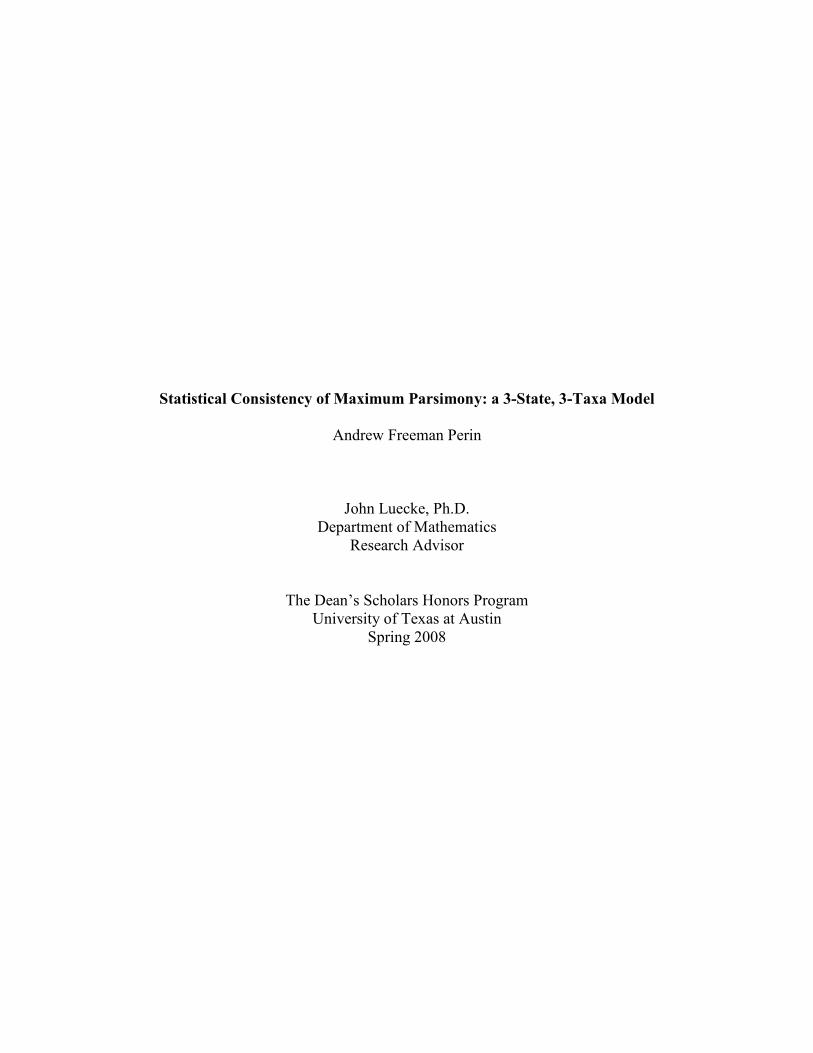
phylogenetic method. The model considers the following evolutionary tree:

Perin 3

(Felsenstein 403)

Here evolution occurs along edges I-V resulting in species A, B, and C. The values P, Q, and R

indicate the probability of changing from one base pair to another along the corresponding edge.

Intuitively, this change represents a mutation in DNA sequence that leads to creation of a new

species. By analyzing maximum parsimony under this model, we find that by varying the

probabilities of changing along an edge, the maximum parsimony method can become

inconsistent and predict the incorrect tree.

Background:

The study of phylogenetics attempts to recover and decipher information about how

species have evolved over time. By making certain assumptions about how evolution can occur,

mathematicians can develop methods to compare the relationships between modern species to

make conclusions about common ancestry. These methods will possess varying statistical

properties, notably that of consistency. Let X1, X2, X3,…, Xn be a sample of size n from a

particular probability distribution. These could be the set of a class’s test scores, for example. For

some parameter θ that represents information about the probability distribution, some function of

the samples can be used to estimate θ. Let En = f(X1, X2, X3,…, Xn) be such an estimator of θ.

For example, θ might be the true average that students should score on an exam and En could be

the calculated mean for the class’s test scores. If E is a consistent estimator, then for any ε > 0,

Perin 4

the limit as n→∞ of P( |En – θ| ≥ ε) = 0, where P(A) = the probability that event A will occur. In

other words, no matter how small we choose ε to be, the probability that the difference between

the estimator, En, and the true parameter, θ, is greater than ε approaches 0 as the size of our

sample grows to infinity. So if an estimator is consistent it will converge upon the true value of

the parameter as the sample size gets larger and larger.

In phylogenetics, the estimator is the phylogenetic tree inferred, the parameter being

estimated is the true tree (i.e. the tree that represents how evolution actually occurred over time)

and the sample is the collection of gene sequences being compared to create the tree. Thus when

we say that an estimator is consistent, we mean that as the length of the gene sequence grows

larger, the tree produced converges upon the true tree. Being able to accurately predict a tree

given a large data set is clearly desirable, and thus we can use consistency as a guideline for

evaluating the performance of an estimation method.

In general, the methods used to determine ancestry produce a phylogenetic tree, a

specialized type of graph. We will introduce some general definitions before we can dive into the

method of maximum parsimony and relevant literature. A graph is a set of vertices and the edges

that connect those vertices.

Figure 1 A generalized graph depicting a set of vertices V = {v1, v2, v3, v4, v5}

and a set of edges E = {(v1, v2), (v2, v3), (v2, v4), (v3, v4)}. Vertex v5 is isolated.

Perin 5

In the above example, there is a set of five vertices and four edges. Notice that it is possible for a

vertex to be isolated and untouched by any edge, like v5. The degree of a vertex is the number of

edges that are incident, or connected, to it. For example, the degree of v2 is 3, because it has 3

edges connected to it. A cycle is defined to be a set of vertices and edges such that you can start

at one vertex, move to the next and so on, and then move from your final vertex back to the

starting vertex. In the example above, vertices v2, v3, and v4 form a cycle. With these definitions

in mind, a tree is defined as a graph with no cycles in which all vertices have degree of at least 1.

A vertex on a tree is called a leaf if it has degree one, and any vertex that is not a leaf is called an

interior vertex.

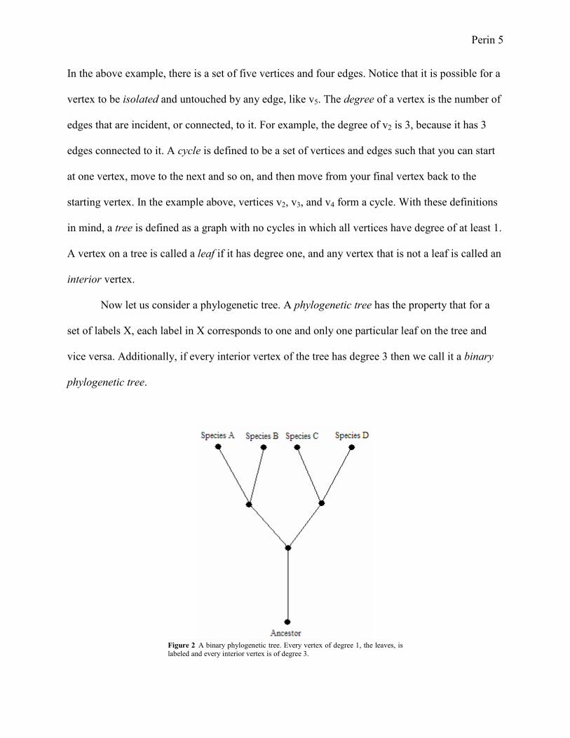
Now let us consider a phylogenetic tree. A phylogenetic tree has the property that for a

set of labels X, each label in X corresponds to one and only one particular leaf on the tree and

vice versa. Additionally, if every interior vertex of the tree has degree 3 then we call it a binary

phylogenetic tree.

Figure 2 A binary phylogenetic tree. Every vertex of degree 1, the leaves, is labeled and every interior vertex is of degree 3.

Perin 6

In the above example of a binary phylogenetic tree, we have labeled all of the leaves and left the

interior vertices unlabelled. The root indicates the common ancestor of all of the leaves, the first

speciation event. Binary phylogenetic trees seem to best represent how evolution actually occurs.

The biological interpretation of a binary phylogenetic tree is that a species will evolve into two

distinct species. For example, consider an animal population that was separated by some natural

event, like the gradual division of land by formation of a river (this occurred with the formation

of the Grand Canyon). Once that population becomes separated, each resulting group will be

subjected to different pressures that select for various traits existing in that species. Eventually

these two groups can evolve into two entirely different species that descended from a common

ancestor. Thus it makes sense to develop methods that generate binary phylogenetic trees.

Having defined the binary phylogenetic tree, we will turn to the consideration of

character and character states. Mathematically, a character on X, is a function, χ, that maps from

X into a set C of character states (Semple 65). X is the set of labels of the leaves of the

phylogenetic tree under consideration, and the set C contains all of traits that the leaves might

take. Biologically, a character can be a particular trait or even a particular position of a DNA

sequence (Semple 65). Consider the example of the character being a nucleotide position of a

gene sequence. In this case, the set X would represent all of the species being compared, and C

would represent all of the possible states that the nucleotide position could take, in this case A,

G, T, or C (adenine, guanine, tyrosine, and cytosine). The character χ would take a member of X

and assign it a state from C. Note that for a phylogenetic tree only the leaves are labeled and

assigned character states. The interior vertices remain unlabelled. The interior vertices are

essentially the ancestors of the leaves, so we need to consider what states these vertices would

take.

Perin 7

For a particular tree T, label set X, character χ, and state set C, we can define an extension

of χ as a function that assigns character states to the interior vertices of the tree without altering

the states of the leaves. Essentially, the extension fills in the missing information and assigns

character states to the ancestors. Once an extension is applied and the interior vertices are

assigned character states, we can define the changing set as the set of all edges of the tree such

that the vertices incident to that edge have different character states. The changing number is the

number of edges in the changing set. So for a given tree and extension, the changing number tells

us how many times there was a change along an edge from one character state to another. The

parsimony score of χ on the tree is the minimum value of the changing number over all possible

extensions. To calculate the parsimony score, we simply consider all of the possible extensions

of χ, choose an extension that minimizes the number of changes that occur along any edge (the

minimum extension), and count the number of changes.

(Semple 85)

Figure 3 A minimum extension for a binary phylogenetic tree, T. With X =

{1, 2, 3, 4, 5} and C = {α, β, γ}, the tree is labeled by χ: X → C. χ(1) = χ(5) = α, χ(3) = χ(4) = β, and χ(2) = γ. The minimum extension of χ assigns labels to

the interior vertices of T so that the changing number is the lowest possible.

The parsimony score is given by this value, and in this case we get a score of 3 (Count the dotted lines). Notice that a minimum extension is not unique; we

could label the rightmost interior vertex γ instead of α and still get the same

changing number.

For a particular gene sequence that we are comparing among several species, we can define each

nucleotide position in the sequence as a single character taking character states A, G, T, and C.

For a gene of length n, we have a sequence of n characters, C = (χ1, χ2, χ3,…, χn). We can then

Perin 8

independently calculate the parsimony score for each character and define the parsimony score

of C on the tree T as the sum of the parsimony scores of each character in C. The tree that

minimizes the parsimony score is defined as the maximum parsimony tree for C.

We now have a method for determining the maximum parsimony tree for a given set of

species. By comparing the gene sequences for the set of species, we can calculate the parsimony

scores for all of the possible phylogenetic trees of the species and choose the tree that minimizes

the score. Note that such a minimal tree is not necessarily unique, as shown in Figure 3.

In a paper published in Systematic Zoology, 1978, Joseph Felsenstein derived an example

where the maximum parsimony method can be an inconsistent estimator of a phylogenetic tree,

even when restricted to three taxa, or groups/species being compared. As this paper forms a basis

on which this study was conducted, it is worthwhile to describe it in detail. Felsenstein’s

example uses a simplified evolutionary model in which there are two character states, 0 and 1,

analogous to a theoretical situation of having DNA with only two possible nucleotides. Evolution

of species occurs via the Camin-Sokal method, which assumes that evolution is irreversible -

once a character evolves into a particular state it cannot revert back to its original state (Camin

312). In Felsenstein’s paper, this assumption is applied as follows: a change in character state

can only occur from 0→1, and once a character takes state 1, it cannot revert back to state 0. As

a result, any descendent of a character assigned state 1 will also be in state 1 (Felsenstein 403).

The tree being analyzed is shown in the following diagram.

Perin 9

(Felsenstein 403) Figure 4 A three-taxa binary phylogenetic tree. Evolution occurs along edges

I, II, III, IV, and V to give rise to species A, B, and C. P, Q, and R denote the

probability that a character will change state along the designated edge.

Here we consider three species, A, B, and C, that have evolved from a common ancestor.

Assume that the diagram gives the correct relationship of the species with A and B being the

most closely related (this relationship is denoted (AB)C). The values P, Q, and R represent the

probabilities of changing character states from 0→1 along their corresponding edges. These are

assumed to be the same for each character, i.e. each nucleotide position, of the sequences being

analyzed. We will define the ancestor at the root of the tree to be in state 0. Thus the probability

of changing from state 0 to state 1 along edge I is given by the probability R. Because they are

probabilities, 0 ≤ P, Q, R ≤ 1. Since we know the probability of changing character states along

any edge, we can calculate the probabilities of the character having certain arrangements of

character states. From now on, we will describe a character as a sequence of character states in

order from A to B to C. For example, if we want to know the probability of a particular character

taking configuration 000 (A has state 0, B has state 0, and C has state 0), then we simply have to

find the probability that there is no change along any of the edges. This probability is given by

P000 = (1 – R)(1 – P)2(1 – Q)

2.

The other possibilities require a bit more consideration. For example, the configuration 001

means that we cannot have any changes along the edges before species A or species B, but that

Perin 10

change must occur before species C. The only way to achieve this is if no change occurs along

edges I, II, III, and IV, but there is a change along edge V. The result is

P001 = P(1 – P)(1 – Q)2(1 – R).

For a state that requires two changes, we need to be even more careful, considering all of the

ways we could achieve those states. Consider the state 110. Since species C is in state 0, there

cannot be any changes along edges I and V. Because both species A and B take on state 1, it

could be that their common ancestor was already in state 1 for that particular character OR

species A and B evolved that character state independently from their common ancestor in state

0. Accordingly, we have to sum the probabilities of each of these events conditionally, so we

need to calculate P(110 | change along edge II) + P(110 | no change along edge II). Note: the

notation P(event X | event Y) means the probability that event X occurs given that event Y also

occurs. Thus,

P110 = (1 – R)[Q + (1 – Q)PQ](1 – P).

We can calculate the probabilities for all 8 of the possible character states to arrive at the

following probabilities. The confirmation of these probabilities will be left as an exercise for the

reader.

P000 = (1 – R)(1 – P)2(1 – Q)

2

P001 = P(1 – P)(1 – Q)2(1 – R)

P010 = (1 – P)2Q(1 – Q)(1 – R)

P100 = P(1 – P)(1 – Q)2(1 – R)

P011 = P(1 – P)Q(1 – Q)(1 – R)

P110 = (1 – R)[Q + (1 – Q)PQ](1 – P)

P101 = P2(1 – Q)

2(1 – R)

P111 = PQ[P(1 – Q) + 1](1 – R) + R

In the remaining portion of the paper, the notion of maximum parsimony is converted to a

statistical problem. Let us consider N characters in the three species, i.e. we are looking at a

sequence of N nucleotide positions in the genes of species A, B, and C. We can count how many

Perin 11

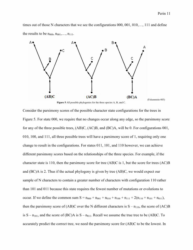
times out of those N characters that we see the configurations 000, 001, 010,…, 111 and define

the results to be n000, n001,…, n111.

(Felsenstein 403) Figure 5 All possible phylogenies for the three species A, B, and C.

Consider the parsimony scores of the possible character state configurations for the trees in

Figure 5. For state 000, we require that no changes occur along any edge, so the parsimony score

for any of the three possible trees, (AB)C, (AC)B, and (BC)A, will be 0. For configurations 001,

010, 100, and 111, all three possible trees will have a parsimony score of 1, requiring only one

change to result in the configurations. For states 011, 101, and 110 however, we can achieve

different parsimony scores based on the relationships of the three species. For example, if the

character state is 110, then the parsimony score for tree (AB)C is 1, but the score for trees (AC)B

and (BC)A is 2. Thus if the actual phylogeny is given by tree (AB)C, we would expect our

sample of N characters to contain a greater number of characters with configuration 110 rather

than 101 and 011 because this state requires the fewest number of mutations or evolutions to

occur. If we define the common sum S = n000 + n001 + n010 + n100 + n111 + 2(n110 + n101 + n011),

then the parsimony score of (AB)C over the N different characters is S – n110, the score of (AC)B

is S – n101, and the score of (BC)A is S – n011. Recall we assume the true tree to be (AB)C. To

accurately predict the correct tree, we need the parsimony score for (AB)C to be the lowest. In

Perin 12

order to achieve this, we need n110 to be the largest of the observed data. Thus we will predict the

correct tree (AB)C if and only if n110 > n101 AND n110 > n011, which can be rewritten as n110 >

n101, n011.

Now that we have a condition necessary for predicting the correct tree, we can convert

this condition into probabilistic terms in order to make use of the previously calculated

probabilities in terms of P, Q, and R. To do so, we apply the Strong Law of Large Numbers.

Consider a situation where you take data samples and calculate the average of your samples. The

Strong Law of Large Numbers states that as the size of the sample increases, the sample mean

(the calculated average) will approach the true mean, or the actual average that you are trying to

estimate. Mathematically, if µsample is the sample mean, and µ is the true mean, then for a sample

of size n, as n→ ∞, µsample→ µ. In phylogenetics, we can think of each of the N characters as

independent events, assuming that the mutation of one base pair is not influenced nor influences

the mutation of another. The N character configurations thus form a random sample of size N.

Now we can apply a version of the Strong Law of Large Numbers to conclude that with

probability 1, as N→ ∞ (as we consider more and more characters, i.e. the gene length grows),

the proportion of times the configuration ijk is observed will converge upon the true probability

of achieving that character state, Pijk. That is, as N→ ∞, nijk/N→ Pijk. Accordingly, for large

values of N the previous condition for predicting the correct tree, n110 > n101, n011, is converted to

the condition that P110 > P101, P011. We have already calculated these probabilities in terms of P,

Q, and R, so now we can simply consider what values of these constants will cause the inequality

not to hold. First, the inequality P110 > P011 reduces to Q(1 – P) > 0, which always holds as 0 < P,

Q < 1. The more interesting case is P110 > P101, which is equivalent to

P2(1 – Q) + PQ

2 – Q < 0.

Perin 13

Notice that this is a quadratic equation in P with coefficients in terms of Q. The relevant solution

to this equation is given by P < (-Q2 + [Q

4 + 4Q(1 – Q)]

1/2) / 2(1 – Q). By plotting this function,

we can observe when this inequality does not hold. In such a situation, we will no longer predict

the correct tree even if the number of characters under comparison is large.

(Felsenstein 405)

Figure 6 A plot of P = (-Q2 + [Q4 + 4Q(1 – Q)]1/2) / 2(1 – Q). Taking values of P and Q below the curve result in accurate prediction of the phylogenetic tree.

Values above the curve in the region labeled NC lead to inconsistency and

false prediction of the phylogeny.

If P and Q fall in the region labeled NC, then, with probability 1, as N→∞, n110 > n101, n011 will

no longer hold. Thus values of P and Q in the NC region will lead to an inconsistent

implementation of maximum parsimony. This region has since been defined as the Felsenstein

zone.

By converting the maximum parsimony method into a statistical, probabilistic problem,

Felsenstein was able to apply the law of large numbers to show an example where maximum

parsimony can be inconsistent. Following Felsenstein’s lead, we will consider the same general

3-taxa tree. However, instead of assuming a Camin-Sokal method of evolution with two possible

character states we will consider the case of three possible character states where the evolution of

a character is reversible.

Perin 14

Results:

We extend Felsenstein’s example and alter the mode by which evolution occurs. We now

consider a model with 3 states (0, 1, and 2) and 3 taxa (A, B, and C). All possible state changes

can occur, i.e. we have 0↔1, 1↔2, 0↔2 allowed as reversible mutations. This mode of

evolution seems to be more plausible than the Camin-Sokal mode because there is no biological

restriction placed on a nucleotide position that prevents it from reverting to an original state once

it has mutated. Furthermore, a change in an individual nucleotide does not necessarily imply a

visible change in a gene product, as three nucleotides are required to code for a particular amino

acid. As such, it is possible that a mutation of a particular nucleotide has no effect on the gene

product and would be able to revert back to an original state without violating the assumptions

that Camin and Sokal make.

In addition to allowing reversions to occur, we assume that the evolutionary process can

be modeled in a Markov fashion. A process is defined as an infinite sequence of random

variables indexed by the natural numbers, {Xn}nε�. A process is considered to be Markov if the

probability of achieving a certain state at a given time or step depends solely on the time or step

that immediately precedes it. Formally, we say a process is Markov in nature if for a process

{Xn}, P[Xn+1 = in+1 | Xn = in, Xn-1 = in-1,…, X1 = i1, X0 = i0] = P[Xn+1 = in+1 | Xn = in]. Thus the

probability that the process is in state in+1 at time n+1 is conditioned only on the state at time n,

and is not affected at all by any other states. For example, consider the process of a baseball

player running the bases. We can think of each time step as a hitter coming up to bat. The

probability that a runner on second base moves to either third base or scores at home plate

depends only on what the next hitter does. In calculating those probabilities, we do not have to

Perin 15

consider how that runner made it to second base at all. All we need to know is that he starts at

second base at time n to consider if he will make it to third base or home plate at time n+1. It

does not matter if he made it to second base via a double or a single and a steal or a single and

another player’s hit, etc, because these things do not affect how the player will run in future

steps.

Accordingly, we can think of evolution as a Markov process. Whatever state a particular

nucleotide position takes at time n+1 depends only on the state of that position at time n. If we

can calculate all of the conditional probabilities that a character is in a particular state at a

particular time, then we can assemble a transition matrix that reflects all of the possible outcomes

of the evolutionary process. Each position in the matrix will reflect the probability of changing

from one state to another, or in the case of the diagonal of the matrix, the probability of having

no change occur. For our example, we assemble a transition matrix along each edge. For edge I,

the probability of changing from one state to another is R. Thus the probability of no change is 1

- 2R, so that the sum of the probabilities of all possible outcomes is 1. The result is a 3x3

transition matrix, R, of the form

(1-2R R R)

(R 1-2R R)

(R R 1-2R).

The ijth entry (row i, column j) gives the probability of changing from state i to state j along edge

I. For example, look at the first row above. This row represents all possible outcomes if the root

is in state 0. Entry R11 gives the probability of staying in state 0, entry R12 gives the probability

of changing from state 0 to state 1, and entry R13 gives the probability of changing from state 0

to state 2. Thus the rows represent the state at time n, and the columns represent the state at time

n+1. For all other edges, we have a similar transition matrix with R replaced by the

corresponding probability of changing along that edge (P or Q). If we know the initial

Perin 16

distribution of states then we can assemble a row vector and multiply it on the right by the

transition matrix to determine the probability of achieving each state. The initial distribution

gives the probability of starting in a particular state. If we know what state we start in, then the

row vector entries of this initial distribution will be 1 for that state and 0 for all others. In our

analysis, we arbitrarily select state 0 to be the root. It makes no difference what state we select as

the ancestor in Figure 4 because there is symmetry in transitions for each state of the Markov

process. Switching the ancestral state would be analogous to renaming each state but analysis

would yield the same results. Thus to get the probability of achieving each state after edge I we

simply multiply the initial distribution by the transition matrix. The result of multiplying a 1x3

row vector by a 3x3 transition matrix is a 1x3 row vector, and thus we can think of the process of

multiplication as the generation of the new probability distribution for the next vertex along the

edge.

Thus to determine the probability that a character is in a certain state at a given vertex, we

can simply take our initial distribution and multiply it by all of the transition matrices that

correspond to the edges that precede that vertex. So for the leaves A, B, and C of the

phylogenetic tree we are analyzing, we get the following probability distributions:

DistA = ((α¯.R¯).Q

¯).P

¯

DistB = ((α¯.R¯).Q

¯).Q

¯

DistC = (α¯.R¯).P

¯

α¯

is the initial distribution, and the dots represent matrix multiplication. The probability of

achieving configuration 000 would be the product of the first entries of DistA, DistB, and DistC.

For any i, j, k where i, j, and k are 0, 1, or 2, we can calculate Pijk by multiplying the ith

entry of

DistA, the jth

entry of DistB, and the kth

entry of DistC. We can now compare these probabilities in

a similar fashion to Felsenstein’s two-state model.

Perin 17

In order to accurately predict the correct tree using the maximum parsimony method, we

must consider the parsimony scores for all possible trees to see which character configurations

have differing scores. For most configurations, whatever phylogeny we choose will have the

same parsimony scores. For some configurations, however, the parsimony score will vary based

on the phylogeny we choose. The following table shows the varying scores for each possible

phylogeny, (AB)C, (AC)B, and (BC)A.

Configuration (AB)C (AC)B (BC)A

011 2 2 1

101 2 1 2

110 1 2 2

022 2 2 1

202 2 1 2

220 1 2 2

Figure 7 For each possible phylogeny of species A, B, and C, the parsimony score for six states is given. For each of these six states, one of the given

phylogenies will possess a lower parsimony score than the other two.

Just as in Felsenstein’s paper, we can compare the probabilities of achieving each state to

determine when maximum parsimony will be inconsistent for this model. Again with respect to a

common value, S, we have that (AB)C is predicted when S – n110 – n220 is smaller than S – n101 –

n202 and smaller than S – n011 – n022. Thus we will correctly predict phylogeny (AB)C when n110

+ n220 > n011 + n022, n101 + n202. If either condition fails, we will predict the wrong tree. In other

words, we will arrive at the correct phylogeny when those configurations requiring the fewest

changes of those in the Figure 7, for which (AB)C is the most parsimonious tree, are observed in

greater frequency. By applying the Strong Law of Large Numbers, the above inequality can be

converted to terms in P, Q, and R. Thus to accurately predict tree (AB)C, we must have P110 +

P220 > P011 + P022, P101 + P202.

Perin 18

First we will consider P110 + P220 > P011 + P022. In terms of P, Q, and R, this inequality

becomes (3P - 1)Q(3R - 1)(R + Q(3Q - 2)(3R - 1)) > 0. We want to find values of P, Q, and R

such that this inequality does not hold. For these values, maximum parsimony will be

inconsistent. Because Q is always positive, we can ignore it, reducing our inequality to (3P -

1)(3R - 1)(R + Q(3Q - 2)(3R - 1)) > 0. This inequality will fail when either 1 or all 3 of the

quantities on the left-hand side are negative. The quantity (3P - 1) is negative for P < 1/3. The

quantity (3R - 1) is negative for R < 1/3. The quantity (R + Q(3Q - 2)(3R - 1)) is negative for R

< (Q(3Q - 2))/(3Q - 1)2. Combining all of these conditions, we can visualize the results in three

dimensions. When P, Q, and R take values in the regions marked C, the first condition for

consistency is satisfied. For the regions marked NC, there is inconsistency.

Perin 19

Figure 8: P110 + P220 > P011 + P022 The two graphs provide different view points of the boundary surfaces for the

inequality (3P - 1)Q(3R - 1)(R + Q(3Q - 2)(3R - 1)) > 0. The regions labeled

NC designate values of P, Q, and R that will result in an inconsistent result, an incorrect prediction of the phylogeny.

Notice that by moving across any of the surfaces, we switch from a region of consistency to a

region of inconsistency and vice versa. Thus there are values of P, Q, and R we can take that will

cause maximum parsimony to be inconsistent and incorrectly predict the phylogeny for our

model under this first condition.

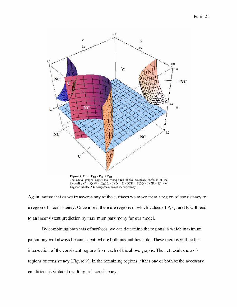
Now let us consider the second inequality, P110 + P220 > P101 + P202. This reduces to

Perin 20

(P + Q(3Q - 2))(3R - 1)(Q + R - 3QR + P(3Q - 1)(3R - 1)) > 0. Again, there are three quantities

to consider on the left-hand side, and when either 1 or all 3 of these are negative, the inequality

will fail and there will be inconsistency. We can map the surfaces given by each quantity to

determine the boundaries for consistent/inconsistent regions for the second condition:

Perin 21

Figure 9: P110 + P220 > P101 + P202

The above graphs depict two viewpoints of the boundary surfaces of the inequality (P + Q(3Q - 2))(3R - 1)(Q + R - 3QR + P(3Q - 1)(3R - 1)) > 0.

Regions labeled NC designate areas of inconsistency.

Again, notice that as we transverse any of the surfaces we move from a region of consistency to

a region of inconsistency. Once more, there are regions in which values of P, Q, and R will lead

to an inconsistent prediction by maximum parsimony for our model.

By combining both sets of surfaces, we can determine the regions in which maximum

parsimony will always be consistent, where both inequalities hold. These regions will be the

intersection of the consistent regions from each of the above graphs. The net result shows 3

regions of consistency (Figure 9). In the remaining regions, either one or both of the necessary

conditions is violated resulting in inconsistency.

Perin 22

Figure 10 The above graph depicts the intersection of the consistent regions

from P110 + P220 > P011 + P022 and P110 + P220 > P101 + P202. Any other region

will be inconsistent due to failure of either one or both of the necessary inequalities.

Discussion:

The results of the consistency analysis for maximum parsimony in a 3-state, 3-taxa model

under reversible character evolution corroborated the results reached by Felsenstein. The

estimation method proved to be inconsistent for certain values of P, Q, and R. These values

covered regions where both P and R were large and Q small, where Q was large and P was small,

and where P and Q were small but R was large. When P is large and Q is small, the inconsistency

result is equivalent to that found by Felsenstein. Essentially, inconsistency occurs when parallel

changes along distinct edges are more probable than change on a single edge (Felsenstein 408).

The interesting result from this analysis is that the value of R affected the consistency of the

estimation method whereas in the Camin-Sokal method of evolution R was negligible. We find

Perin 23

that when R is large and P and Q are both small we can have an inconsistent result. This follows

from the fact that the ancestor evolved after any mutation along edge I with probability R will

cause the resulting species to take on that state. The character states that possessed different

parsimony scores were characterized by two species taking the same state, either 1 or 2, and a

third remaining at state 0. In the event that a mutation occurs with high probability along edge I,

it is very feasible for one of those states to then revert back to state 0 along edge III, IV, or V.

Although consistency is a desirable trait for a phylogenetic estimator to possess, we must

evaluate consistency with respect to other features and considerations of estimators. Estimation

methods should also be efficient, powerful, robust, and falsifiable (Penny 73). Efficiency refers

to speed. Currently, just as with parsimony, most phylogenetic methods require optimization on a

single tree and then determination of a global optimum over all trees (Penny 74). For example,

the determination of a maximum parsimony tree from a set of species is an NP-hard problem.

Alternatively, it is much easier to calculate the parsimony score once given a tree, and this can be

achieved in polynomial time. As a result, parsimony is only practically applicable for the

comparison of up to 30 species before it becomes too computationally taxing (Kim 6). The

power of a method refers to the length of DNA sequences required before convergence on a

result (Penny 74). If a given method is powerful, it will converge upon a result quickly. A robust

method is powerful and consistent, even with significant deviations from the model (Penny 76).

For example, if observed data does not reflect assumptions made by a given model, the model

will be considered robust even if it is still able to predict a tree powerfully and consistently.

Finally, a good phylogenetic method should be falsifiable in that “data must…be able to reject

the model,” though few methods meet this requirement (Penny 76). It is not currently feasible for

Perin 24

any given method to possess all five of these characteristics, but all should attempt to find some

balance between them.

With this in mind, we must recognize that inconsistency does not necessarily signify

failure of a model for predicting the phylogeny of a set of species. Conversely, consistency does

not imply success alone but must be evaluated with other characteristics in mind. Overall, how

well a particular model performs is a measure of how well a particular method’s assumption of

how evolution occurs approximates how evolution actually occurs. It has been shown that most

phylogenetic methods rely on assumptions that are violated by real-world data, so we must

evaluate phylogenetic methods by their performance in lieu of such violations (Hillis 259). We

can use real-world data to evaluate if the maximum parsimony method will be susceptible to

violation of any assumptions.

In this analysis we have extended Felsenstein’s 2-state, 3-taxa model depicting instances

of inconsistency of maximum parsimony into a 3-state, 3-taxa model with different assumptions

about evolutionary constraints. Even when there are no restrictions on the process of evolution,

when mutations are reversible, it is indeed possible for maximum parsimony to be inconsistent

and converge upon the incorrect phylogeny as the gene sequence grows without bound.

Perin 25

References:

Camin, Joseph H., and Robert R. Sokal. "A Method for Deducing Branching Sequences in

Phylogeny." Evolution 19.3 (Sept. 1965): 311-326.

Felsenstein, Joseph. "Cases in Which Parsimony or Compatibility Methods Will Be Positively

Misleading." Systematic Zoology 27.4 (Dec. 1978): 401-410.

Hillis, David M., John P. Huelsenbeck, and David L. Swofford. "Hobgoblin of Phylogenetics?"

Nature 369 (June 1994): 363-364.

Huelsenbeck, John P., and David M. Hillis. "Success of Phylogenetic Methods in the Four-

Taxon Case." Systematic Biology 42.3 (Sept. 1993): 247-264.

J. Kim and T. Warnow. 1999. Tutorial on Phylogenetic Tree Estimation. Intelligent Systems for

Molecular Biology, Heidelberg 1999.

C.R. Linder, and T. Warnow, 2005. "Overview of Phylogeny Reconstruction." Book chapter, in

S. Aluru (editor), Handbook of Computational Biology, Chapman & Hall, CRC

Computer and Information Science Series, 2005.

Semple, Charles, and Mike Steel. Phylogenetics. New York: Oxford University Press, 2003.

Penny, David, Michael D. Hendy, and Michael A. Steel. "Progress with Methods for

Constructing Evolutionary Trees." Trends in Ecology and Evolution 7 (1992): 73-79.

Steel, Michael A., Michael D. Hendy, and David Penny. "Parsimony Can be Consistent!"

Systematic Biology 42.4 (Dec. 1993): 581-587.