Facolta di Scienze e Tecnologie

Laurea Triennale in Fisica

Angle resolved scattering

of strong-field

electromagnetic radiation

Relatore: Prof. Nicola Manini

Correlatore: Prof. Giovanni Onida

Simone Trevisan

Matricola n 830220

A.A. 2015/2016

Codice PACS: 78.70.Ck

Angle resolved scattering

of strong-field

electromagnetic radiation

Simone Trevisan

Dipartimento di Fisica, Universita degli Studi di Milano,

Via Celoria 16, 20133 Milano, Italia

February 23, 2017

Abstract

We simulate X-ray scattering beyond perturbation theory, relevant for X-

ray free electron laser (XFEL) pulses. Previous work by Mattia Mantovani im-

plemented a numerical solution of the exact Schodinger equation involving the

full coupling of an electron dynamics with the vector potential of an ultrashort

electromagnetic pulse.

Our thesis reaches a further step in this Maxwell-Schrodinger model, pro-

viding a theoretical discussion and a numerical implementation of the calculation

of the far-field scattering angular pattern, given the current density as obtained

from Mantovani’s code. Our predictions are in good accord with the perturba-

tive results for small to intermediate pulse average intensities, whereas we observe

non-linear effects beyond 1027 W m−2. We relate our results to the Keldysh pa-

rameter γ, which estimates inversely the prevalence of field-induced tunneling

ionization: a large value of the parameter compared to 1 is often taken as a justi-

fication for perturbative methods. Our results confirm that non linear effects are

observed when γ < 1.

Advisor: Prof. Nicola Manini

Co-Advisor: Prof. Giovanni Onida

Contents1 Introduction 5

2 State of the art 9

2.1 The Schrodinger approach . . . . . . . . . . . . . . . . . . . . . . 9

2.1.1 Minimal coupling Hamiltonian . . . . . . . . . . . . . . . . 9

2.1.2 Gauge choice . . . . . . . . . . . . . . . . . . . . . . . . . 10

2.1.3 Charge and current density . . . . . . . . . . . . . . . . . 11

2.2 X-ray scattering in the perturbative limit . . . . . . . . . . . . . . 12

2.3 The Keldysh parameter . . . . . . . . . . . . . . . . . . . . . . . . 13

3 Radiation from an assigned current density 15

3.1 Radiated electric and magnetic fields . . . . . . . . . . . . . . . . 16

3.2 The Poynting vector and the radiated power . . . . . . . . . . . . 18

3.3 Cross section . . . . . . . . . . . . . . . . . . . . . . . . . . . . . 20

4 The numerical implementation 21

4.1 The Discrete Fourier Transform . . . . . . . . . . . . . . . . . . . 21

4.2 Discretization of space and spatial integration . . . . . . . . . . . 23

4.3 The incoming pulse . . . . . . . . . . . . . . . . . . . . . . . . . . 24

4.4 Convergence . . . . . . . . . . . . . . . . . . . . . . . . . . . . . 26

5 Results 30

5.1 The perturbative limit . . . . . . . . . . . . . . . . . . . . . . . . 30

5.2 High intensities . . . . . . . . . . . . . . . . . . . . . . . . . . . . 31

6 Conclusions and outlooks 36

A Atomic units 38

Ringraziamenti 40

Bibliography 41

3

Al professor Giacinto Biasco,

che mi guarda dal cielo.

Chapter 1

Introduction

Since their discovery in 1895, X-rays evolved into an ever-growing field with

multiple applications in many areas of science and technology. X-rays have proved

to be extremely useful in the investigation of structural properties of matter,

thanks both to their wavelengths (0.01 to 10 nm) which yields the adequate spatial

resolution for imaging nanoscale objects (single atoms, molecules, polymers), and

to their energies (100 eV to 10 keV) which matches inner-shell binding energies,

enabling core absorption, photo-emission and other spectroscopies.

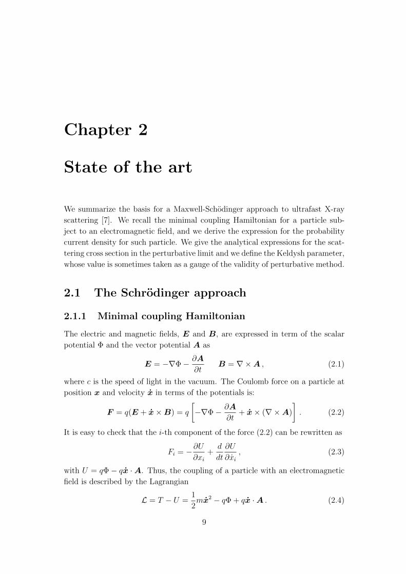
During the past century, special efforts have been made to develop novel

X-ray sources. Techniques have been invented to increase brilliance, monochro-

maticity and coherence of the pulses [1]. In 1947 synchrotron radiation was first

observed, and so the first generation of synchrotron-radiation facilities started,

where X-rays were produced as a parasitic effect in synchrotrones. Soon dedicated

storage rings were built with insertions of devices such as undulators and wig-

glers (second and third generations). Such devices are basically periodic magnetic

structures, that produce a sinusoidal magnetic field. Depending on the strength

and the period of the magnetic field, the radiation produced at every cycle can

sum coherently or incoherently: in the first case the structure is referred to as

an undulator, in the second as a wiggler (Fig. 1.1). These tools allowed to pro-

duce spectrally narrow and collimated pulses: that is, pulses with high spectral

brightness.

In recent years, a fourth generation of X-ray sources has started, thanks to

the invention of free-electron lasers (FELs), which usually are based on very long

undulators inserted in high-energy linear electron accelerators. Such devices can

generate a peak brightness up to 1020 W m−2, many orders of magnitude beyond

that of the previous-generation sources, concentrated in pulses of duration 100 fs

or shorter. FEL pulses are much better spatially coherent than those from syn-

chrotron sources. X-ray free electron lasers (XFELs) in particular have begun

5

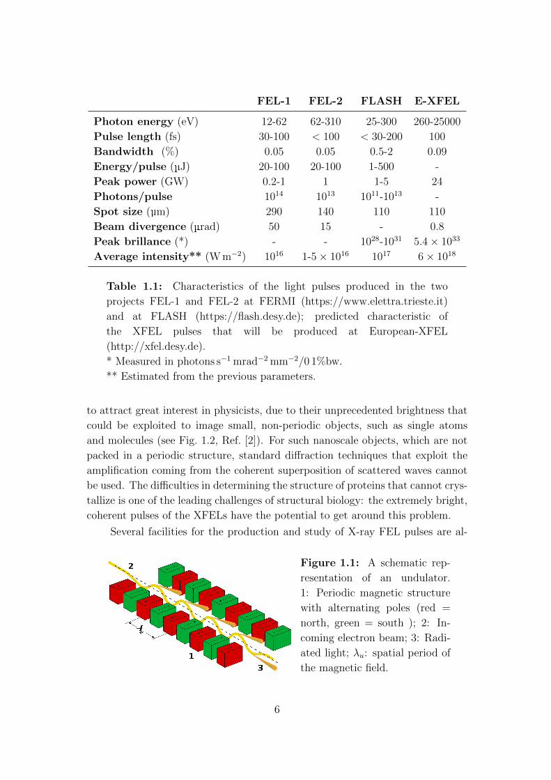
FEL-1 FEL-2 FLASH E-XFEL

Photon energy (eV) 12-62 62-310 25-300 260-25000

Pulse length (fs) 30-100 < 100 < 30-200 100

Bandwidth (%) 0.05 0.05 0.5-2 0.09

Energy/pulse (µJ) 20-100 20-100 1-500 -

Peak power (GW) 0.2-1 1 1-5 24

Photons/pulse 1014 1013 1011-1013 -

Spot size (µm) 290 140 110 110

Beam divergence (µrad) 50 15 - 0.8

Peak brillance (*) - - 1028-1031 5.4× 1033

Average intensity** (W m−2) 1016 1-5× 1016 1017 6× 1018

Table 1.1: Characteristics of the light pulses produced in the two

projects FEL-1 and FEL-2 at FERMI (https://www.elettra.trieste.it)

and at FLASH (https://flash.desy.de); predicted characteristic of

the XFEL pulses that will be produced at European-XFEL

(http://xfel.desy.de).

* Measured in photons s−1 mrad−2 mm−2/0 1%bw.

** Estimated from the previous parameters.

to attract great interest in physicists, due to their unprecedented brightness that

could be exploited to image small, non-periodic objects, such as single atoms

and molecules (see Fig. 1.2, Ref. [2]). For such nanoscale objects, which are not

packed in a periodic structure, standard diffraction techniques that exploit the

amplification coming from the coherent superposition of scattered waves cannot

be used. The difficulties in determining the structure of proteins that cannot crys-

tallize is one of the leading challenges of structural biology: the extremely bright,

coherent pulses of the XFELs have the potential to get around this problem.

Several facilities for the production and study of X-ray FEL pulses are al-

Figure 1.1: A schematic rep-

resentation of an undulator.

1: Periodic magnetic structure

with alternating poles (red =

north, green = south ); 2: In-

coming electron beam; 3: Radi-

ated light; λu: spatial period of

the magnetic field.

6

Figure 1.2: From top left: the diffrac-

tion pattern produced by a microscale

test object investigated by a single FEL

pulse; the pattern of the following FEL

pulse showing the damage to the object

caused by the first pulse; the test object

and its image reconstructed from the

first diffraction pattern using a phase re-

trieval algorithm which does not make

use of the original image.

ready in operation, and other are currently under construction. The FLASH

laboratory (2005) in Hamburg and the FERMI laboratory (2010) in Trieste oper-

ate in the soft X-ray and UV range. In the hard X-ray regime, facilities like LCLS

(USA, 2009), SACLA (Japan, 2012) and PAL-XFEL (South Korea, 2016) are al-

ready in operation, whereas the European-XFEL in Germany and the SwissFEL

in Switzerland are expected to start in 2017 (See Tab. 1.1).

The possibility of single-molecule imaging, however, presents several difficul-

ties. The high intensities of the XFELs pulses is quite likely damage the sample,

that often can undergo a Coulomb explosion, possibly resulting in a deteriorated

or even useless scattering signal. In order to understand these phenomena, sev-

eral theoretical approaches have been used in past years to model the interaction

and predict the scattered radiation pattern, mostly based on perturbation theory

[3]. These methods are usually justified by the small scattering cross section (of

order 10−2 b) and/or by the value of the Keldysh parameter, which estimates the

prevalence of field induced ionization [4]. However, due to the extremely high

intensities of the fields in XFEL pulses, there is no guarantee that the perturba-

tive limit is fulfilled [5]. Non-linear effects may arise, as predicted by theoretical

calculations based on plasma models [6].

The present work fits in this theoretical research, and it is conceived as a

continuation of the previous work by Mattia Mantovani [7], who implemented

and studied a Maxwell-Schrodinger approach to the scattering of ultra-intense,

ultra-fast X-ray pulses from a nano-object. Mantovani set up a numerical solution

of the time-dependent Schrodinger equation for a one-electron atom, subject to

a radiation pulse. The peculiarity of this approach is that the coupling of the

electron dynamics and the radiation does not rely to any weak-coupling or long-

wavelength approximations (specifically, not to the dipole approximation, as was

7

Figure 1.3: A frame from Manto-

vani’s simulations of the real part of

the electron wave function in pres-

ence an electromagnetic pulse propa-

gating in the positive z direction and

polarized along the x-axis. The inner

circle has radius 3a0 ' 1.5 A. Red =

positive wave function; Green = null

wave function; Blue = negative wave

function.

done in previous works). The electromagnetic fields are treated classically, which

is expected to be accurate for the incoming radiation due to extremely high

intensities (and thus great number of photons), but does not take quantum effects

(e.g. the Compton effect) into account.

The Schrodinger equation is solved numerically through finite-element analy-

sis (FEA) employing backward differentiation formulas (BDFs) within a shperical

region which is discretized by a tetrahedral mesh. The solution of the Schrodinger

equation provides both the wave function ψ(x, t) and, as a derived value, the

probability current density j(x, t) (See Fig. 1.3). Both ψ and j are available at

discrete points xi (the vertexes of the tetrahedra) and at discrete, equally spaced

times (tn = n∆t, n = 0, 1, ..., N). The computation of the scattered radiation is

based on the assumption that we can treat the probability current, multiplied by

the electron charge e, as an electric current: the scattered radiation is computed

as the radiation emitted by such current.

In the present work we address the problem of computing the far-field radi-

ation pattern generated by the motion of the electron, given its electric current

density function J(xi, tn) = ej(xi, tn). In Chapter 2 we collect summarize the

Schodinger problem as it is portrayed by Mantovani. In Chapter 3 we describe

the formalism for the main problem of this thesis, obtaining a general expression

for the radiated energy and the differential cross section in the far-field approxi-

mation. In Chapter 4 we describe the numerical implementation and discuss its

convergence. In Chapter 5 we report the results of the application of our method,

comparing them with the formulas of perturbation theory.

8

Chapter 2

State of the art

We summarize the basis for a Maxwell-Schodinger approach to ultrafast X-ray

scattering [7]. We recall the minimal coupling Hamiltonian for a particle sub-

ject to an electromagnetic field, and we derive the expression for the probability

current density for such particle. We give the analytical expressions for the scat-

tering cross section in the perturbative limit and we define the Keldysh parameter,

whose value is sometimes taken as a gauge of the validity of perturbative method.

2.1 The Schrodinger approach

2.1.1 Minimal coupling Hamiltonian

The electric and magnetic fields, E and B, are expressed in term of the scalar

potential Φ and the vector potential A as

E = −∇Φ− ∂A

∂tB = ∇×A , (2.1)

where c is the speed of light in the vacuum. The Coulomb force on a particle at

position x and velocity x in terms of the potentials is:

F = q(E + x×B) = q

[−∇Φ− ∂A

∂t+ x× (∇×A)

]. (2.2)

It is easy to check that the i-th component of the force (2.2) can be rewritten as

Fi = −∂U∂xi

+d

dt

∂U

∂xi, (2.3)

with U = qΦ− qx ·A. Thus, the coupling of a particle with an electromagnetic

field is described by the Lagrangian

L = T − U =1

2mx2 − qΦ + qx ·A . (2.4)

9

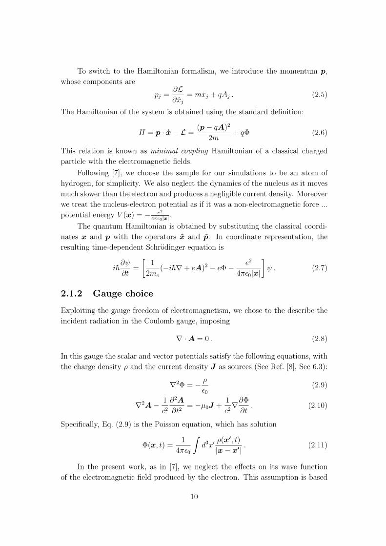
To switch to the Hamiltonian formalism, we introduce the momentum p,

whose components are

pj =∂L∂xj

= mxj + qAj . (2.5)

The Hamiltonian of the system is obtained using the standard definition:

H = p · x− L =(p− qA)2

2m+ qΦ (2.6)

This relation is known as minimal coupling Hamiltonian of a classical charged

particle with the electromagnetic fields.

Following [7], we choose the sample for our simulations to be an atom of

hydrogen, for simplicity. We also neglect the dynamics of the nucleus as it moves

much slower than the electron and produces a negligible current density. Moreover

we treat the nucleus-electron potential as if it was a non-electromagnetic force ...

potential energy V (x) = − e2

4πε0|x| .

The quantum Hamiltonian is obtained by substituting the classical coordi-

nates x and p with the operators x and p. In coordinate representation, the

resulting time-dependent Schrodinger equation is

i~∂ψ

∂t=

[1

2me

(−i~∇+ eA)2 − eΦ− e2

4πε0|x|

]ψ . (2.7)

2.1.2 Gauge choice

Exploiting the gauge freedom of electromagnetism, we chose to the describe the

incident radiation in the Coulomb gauge, imposing

∇ ·A = 0 . (2.8)

In this gauge the scalar and vector potentials satisfy the following equations, with

the charge density ρ and the current density J as sources (See Ref. [8], Sec 6.3):

∇2Φ = − ρε0

(2.9)

∇2A− 1

c2

∂2A

∂t2= −µ0J +

1

c2∇∂Φ

∂t. (2.10)

Specifically, Eq. (2.9) is the Poisson equation, which has solution

Φ(x, t) =1

4πε0

∫d3x′

ρ(x′, t)

|x− x′|. (2.11)

In the present work, as in [7], we neglect the effects on its wave function

of the electromagnetic field produced by the electron. This assumption is based

10

on the principle that an electromagnetic interaction of the electron with itself

is not physical: if it was, the electron would tend to repel itself. Moreover, we

deal with strong-field radiation, with incoming fields that are surely much larger

than the ones produced by the electron, which can be then neglected. With this

assumption, ρ and J in Eq. (2.9) are vanishing, and in particular Φ = 0.

With this gauge choice, Eq. (2.6) is rewritten as

i~∂ψ

∂t=

[− ~2

2me

∇2 − i~ e

me

A · ∇+e2

2me

A2 − e2

4πε0|x|

]ψ . (2.12)

2.1.3 Charge and current density

Here we report the relations between the wave function ψ, obtained numerically

from the solution of Eq. (2.12) and the charge and current density functions:

especially the current density is the basis of our method for calculating the scat-

tering cross section, as we will show in Section 3. For a field-free particle, the

number and number current density operators are defined as

ρ(x) := δ(x− x) (2.13)

j(x) :=1

2ˆx, ρ(x) =

1

2mp, ρ(x) , (2.14)

where ·, · indicates the anticommutator. For one electron, the mean values of

such operators in a normalized state |ψ〉 are

ρ(x) = 〈ψ| ρ(x) |ψ〉 = |ψ(x)|2 (2.15)

j(x) = 〈ψ| j(x) |ψ〉 = − i~2m

[ψ∗(x)∇ψ(x)− ψ(x)∇ψ∗(x)] , (2.16)

and they satisfy the continuity equation (conservation of probability)

∂ρ

∂t(x, t) +∇ · j(x, t) = 0 . (2.17)

Considering now a particle in an electromagnetic field, the definitions Eq. (2.13)

and Eq (2.14) hold the same, and so does Eq. (2.17), but, as one can see from

Eq. (2.5), the current density operator in terms of the canonical momentum p is

different:

j(x) =1

2mp− qA(x), ρ(x) (2.18)

The electric current density for an electron is simply obtained by multiplying by

the charge q = −e the mean value of operator j(x):

J(x, t) = −e 〈ψ, t| j(x) |ψ, t〉 (2.19)

=ie~2m

[ψ∗(x, t)∇ψ(x, t)− ψ(x, t)∇ψ∗(x, t)]− e2

mA(x, t)|ψ(x, t)|2 .

11

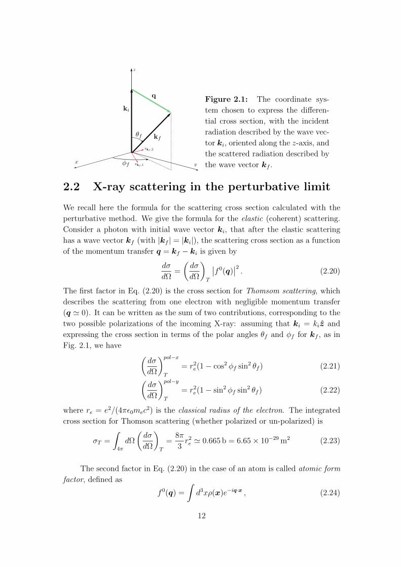
Figure 2.1: The coordinate sys-

tem chosen to express the differen-

tial cross section, with the incident

radiation described by the wave vec-

tor ki, oriented along the z-axis, and

the scattered radiation described by

the wave vector kf .

2.2 X-ray scattering in the perturbative limit

We recall here the formula for the scattering cross section calculated with the

perturbative method. We give the formula for the elastic (coherent) scattering.

Consider a photon with initial wave vector ki, that after the elastic scattering

has a wave vector kf (with |kf | = |ki|), the scattering cross section as a function

of the momentum transfer q = kf − ki is given by

dσ

dΩ=

(dσ

dΩ

)T

∣∣f 0(q)∣∣2 . (2.20)

The first factor in Eq. (2.20) is the cross section for Thomsom scattering, which

describes the scattering from one electron with negligible momentum transfer

(q ' 0). It can be written as the sum of two contributions, corresponding to the

two possible polarizations of the incoming X-ray: assuming that ki = kiz and

expressing the cross section in terms of the polar angles θf and φf for kf , as in

Fig. 2.1, we have (dσ

dΩ

)pol−xT

= r2e(1− cos2 φf sin2 θf ) (2.21)(

dσ

dΩ

)pol−yT

= r2e(1− sin2 φf sin2 θf ) (2.22)

where re = e2/(4πε0mec2) is the classical radius of the electron. The integrated

cross section for Thomson scattering (whether polarized or un-polarized) is

σT =

∫4π

dΩ

(dσ

dΩ

)T

=8π

3r2e ' 0.665 b = 6.65× 10−29 m2 (2.23)

The second factor in Eq. (2.20) in the case of an atom is called atomic form

factor, defined as

f 0(q) =

∫d3xρ(x)e−iq·x , (2.24)

12

where ρ(x) is the ground state electron number density. The form factor for

hydrogen in his ground state is:

f 0(q) =16

(4 + q2a20)2

. (2.25)

As the module of the momentum transfer q is related to the photon energy and

to θf by the relation q = 2ki sinθf2

, the atomic form factor gives an increasingly

important contribution with increasing photon energy: its overall effect is null in

the forward direction, while it tends to suppress the backward scattering (θf = π).

For a photon energy of 10 keV the total cross section, obtained by integrating

Eq. (2.20) over the entire solid angle, is significantly smaller than σT [9]:

σH(~ω0 = 10 keV) ' 41.21 mb ' 0.06σT . (2.26)

2.3 The Keldysh parameter

In a publication dated 1965 [4], L. V. Keldysh proposed a model for ionization

in the presence of monochromatic electromagnetic radiation, and introduced a

parameter that characterizes the dominant ionization process, the Keldysh adia-

baticity parameter :

γ =ω0

√2meIp

eE0

. (2.27)

Here E0 and ω0 are respectively the amplitude and the angular frequency of

the electric field, and Ip is the electron ionization potential for the considered

material.

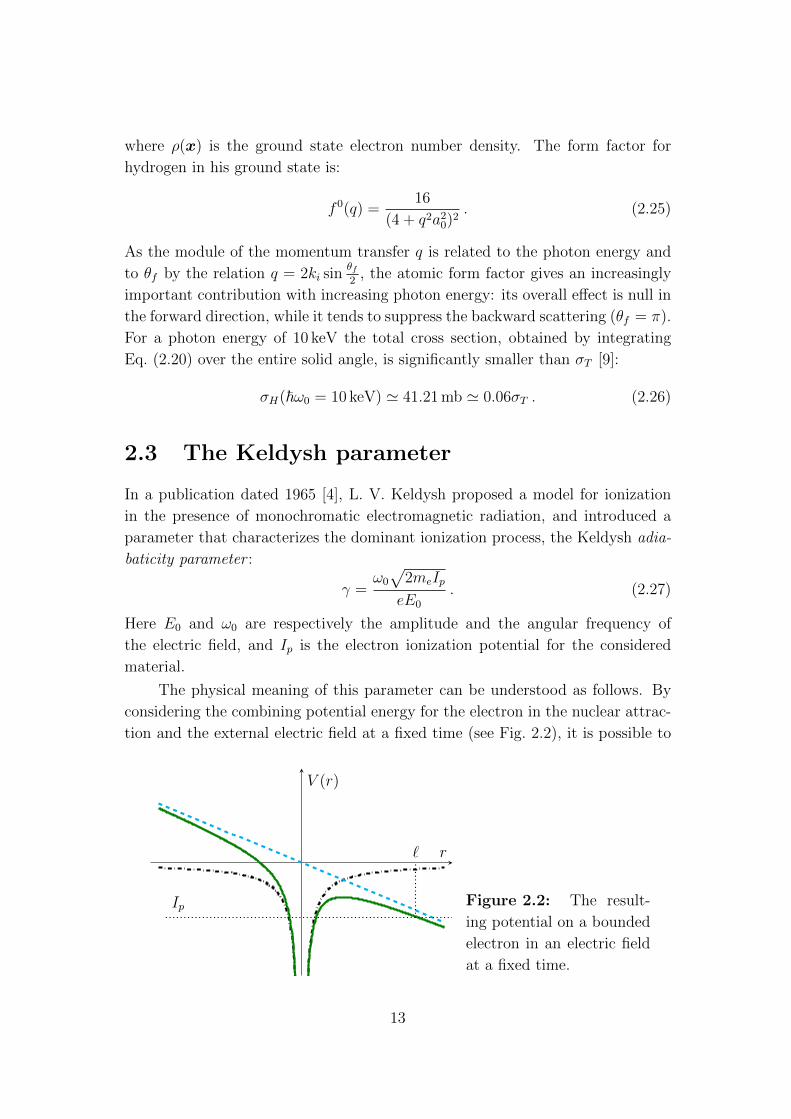
The physical meaning of this parameter can be understood as follows. By

considering the combining potential energy for the electron in the nuclear attrac-

tion and the external electric field at a fixed time (see Fig. 2.2), it is possible to

`

Ip

r

V (r)

Figure 2.2: The result-

ing potential on a bounded

electron in an electric field

at a fixed time.

13

estimate the thickness of the barrier that the electron must overcome to leave the

nucleus as

l =IpeE0

. (2.28)

The mean speed of the electron sitting at a boundstate at energy −Ip is of order

〈v〉 =

√2Ipme

. (2.29)

We can estimate the characteristic time of tunneling as the time that it takes the

electron to pass through the barrier:

τ =l

〈v〉=

1

eE0

√meIp

2. (2.30)

Given the period of the electromagnetic oscillation T0 = 2π/ω0, the Keldysh

parameter (2.27) is proportional to the ratio of the tunneling time τ to the half-

period of the radiation:

γ = 2πτ

T0/2. (2.31)

Tunnel ionization is dominant if τ < T/2, i.e. γ 1, while for τ > T/2 the

electron does not have time enough to tunnel through the barrier.

Keldysh showed that for γ 1 tunnel ionization is dominant, while for

γ 1 ionization can be caused by linear or non-linear processes as single- or

multi-photon ionization, but the tunneling ionization is negligible. When strong

radiation is considered, as in our work, it is useful to evaluate the Keldysh pa-

rameter as a rough estimator of the validity of perturbation theory. It can be fair

to assume that the perturbative limit is fulfilled for γ 1 (negligible tunneling):

as indicated by the definition (2.27), this condition is satisfied for high radiation

frequencies and/or small field amplitude.

14

Chapter 3

Radiation from an assigned

current density

In the present chapter we evaluate the expression for the radiation fields emitted

by a given current density as a function of the observation direction. In this

calculation we assume the hypothesis of far-field radiation: this means that we

assume the current density to vanish outside a restricted region of space, of linear

size d, and that we observe the radiation at a distance r d. This hypothesis

is totally justified in the experimental framework for which the present work is

relevant, where the current density is represented by the motion of the electrons

of a single atom or molecule: such electrons are constrained in a region of at

most a few nanometers (the size of the molecule), whereas the detector cannot

be placed nearer than few centimeters from the sample.

We assume the current density to be localized not only in space, but also in

time, in a time interval 0 to T . Specifically, as previously discussed, we imagine

to deal with an electromagnetic pulse produced by an XFEL, whose durations is

of the order of tens to hundreds of femtoseconds: after the end of the pulse the

molecular system relaxes rapidly, so that the current vanishes again shortly after

the end of the pulse, and before time T it is completely negligible. This is the

only hypothesis that we make: we want to build a theory that makes no further

requirement on the form, amplitude and polarization of the radiation pulse.

15

3.1 Radiated electric and magnetic fields

We start our calculation from the general expression of the vector potential in

the Lorenz gauge (see Ref. [8], Sect.s 6.4 and 6.5):

A(x, t) =µ0

4π

∫d3x′

∫dt′

J(x′, t′)

|x− x′|δ(t′ − t+

|x− x′|c

)

=µ0

4π

∫d3x′

J(x′, t− |x−x′|

c)

|x− x′|, (3.1)

where µ0 is the magnetic permeability of vacuum, related to the electric perme-

ability ε0 and the velocity of light c by the relation c2 = 1/ε0µ0; J is the current

density function; the apostrophized coordinates t′ and x′ refer to the time and

position of emission, while the non-apostrophized t and x refer to the time and

position of observation. The spatial integral in Eq. (3.1) extends in principle over

all space, but since J vanishes outside a compact region of linear size d around

the origin of x space, it can be restricted to that region.

It is convenient to analyze separately the different frequencies of which J

is composed by means of the Fourier theorem. We recall the definition of the

continuous Fourier transform F and of the inverse Fourier transform F−1, which

we use in the present theoretic discussion. (Later on, in the numerical implemen-

tation, we will use the discrete Fourier transform, and we will give the precise

definition also for that.)

f(ω) = F [f ](ω) :=

∫ ∞−∞

dtf(t)e−iωt (3.2)

f(t) = F−1[f ](t) :=1

2π

∫ ∞−∞

dωf(ω)eiωt (3.3)

Here f(ω) indicates the Fourier transform of f(t) from the time-domain to the

frequency-domain, calculated at frequency ω.

According to Eq. (3.3), the general form of J(x, t) is the integral over all

possible frequencies of e−iωt/2π, weighted by the function J(x, ω):

J(x, t) =1

2π

∫ +∞

−∞dωJ(x, ω)eiωt = F−1[J ](x, t) , (3.4)

With the decomposition (3.4), Eq. (3.1) can be rewritten as

A(x, t) =µ0

4π

∫d3x′

∫ +∞−∞ dωJ(x′, ω)e−ik|x−x

′|eiωt/2π

|x− x′|

=µ0

4π

∫ +∞

−∞

dω

2π

∫d3x′

J(x′, ω)e−ik|x−x′|

|x− x′|eiωt , (3.5)

16

with k = ω/c. The retardation effect expressed by the δ-function in Eq. (3.1) has

been wrapped to a frequency-dependent phase factor e−ik|x−x′|. Comparing Eq.

(3.5) with the definition of the inverse FT, Eq. (3.3), we get

A(x, ω) =µ0

4π

∫d3x′

J(x′, ω)e−ik|x−x′|

|x− x′|. (3.6)

In Eq. (3.5) we have changed the order of integration: this is possible thanks

to the fact that our current density function J(x, t) is supposed to be localized

in space and time, and thus every integral, both in time and in space, is granted

to converge (Ref. [10], Ch. 48). This hypothesis also allow us to move the limit

operators from inside to outside the integration symbol and vice versa (Lebesgue’s

dominated convergence theorem [11]), and in particular to change the order of

integrals and derivatives (Ref. [10], Ch. 53). These facts, alongside with the

linearity of the relations between J , A and the fields E and B, Eq. (3.1), (3.10)

and (3.11), are fundamental to ensure us the possibility of making a Fourier

analysis, as we are going to do: we can solve the equations for the fields in the

Fourier space and than go back to the time-domain by an inverse transform, and

that is equivalent to solving the entire problem in the time-domain.

Now we apply the far-field approximation (Ref. [8], Ch. 9), and thus assume

r := |x| |x′|. A first-order Taylor expansions leads to

|x− x′|r

= 1− n · x′

r+ o

(|x′|2

r2

),

where n = x/r is the versor pointing to the direction of observation.

We rewrite Eq. (3.5) in this approximation: in the expansion of 1/|x − x′|we neglect all terms that decay faster than 1/r, as they do not contribute to

far-field radiation, as we will see in Sect. 3.2; in the factor e−ik|x−x′| we expand

|x−x′| neglecting all terms that vanish for r →∞. The equation that we obtain

is:

A(x, ω) ' µ0

4π

e−ikr

r

∫d3x′J(x′, ω)eikn·x

′. (3.7)

Notice that in Eq. (3.7) we do not expand the exponential eikn·x′, as we have not

made any assumption on the relation between the typical size d and the wave-

length of the current, which is similar to the typical wave lengths of the pulse,

related to k by the formula k = 2π/λ. If, for some reason, we could assume λ d

(thus kd 1), we might further expand the factor eikn·x′: that is known as the

multi-polar expansion. Unfortunately, the wave-length of photons with energy

hν ' 10 keV, like the ones that are produced at European-XFEL (see Tab. 1.1),

is ' 1.2 A, comparable to the typical size of the electronic motion.

17

The magnetic field B can be obtained by the formula

B(x, t) = ∇×A(x, t) , (3.8)

which holds also in the frequency domain, with B(x, ω) and A(x, ω). We evaluate

the rotor in spherical coordinates (r, θ, φ) and we take the asymptotic form for

r → ∞, neglecting all terms that decay faster than 1/r because they do not

contribute to far-field radiation. We obtain:

Br(x, ω) ' 0

Bθ(x, ω) ' −ikAφ(x, ω)

Bφ(x, ω) ' ikAθ(x, ω) . (3.9)

The fact that the r-component decays faster than the others reflects the well

known fact that electromagnetic radiation waves in vacuum are transverse. It is

easy to show that the far-field equations (3.9) can be reduced to the following:

B(x, ω) = in× kA(x, ω) . (3.10)

The electric field E(x, t) can be derived from the fourth Maxwell equation,

∇×B(x, t) =1

c2

∂E

∂t(x, t) ,

that in the Fourier representation becomes

E(x, ω) = ic2

ω∇× B(x, ω) , (3.11)

By calculating the rotor of expression (3.10) and making the same approximations

as those made for the magnetic field, we obtain:

E(x, ω) = −cn× B(x, ω) = ic[n× kA(x, ω)]× n . (3.12)

3.2 The Poynting vector and the radiated power

Having derived the far-field expressions for the electric (3.12) and magnetic (3.10)

fields, we can now calculate the Poynting vector S: as we are dealing with complex

fields, we need to define the complex Poynting vector, whose real part represents

the power flux out of an infinitesimal surface orthogonal to its direction (see

Ref. [8], Sect. 6.9).

S(x, t) :=1

2µ0

E(x, t)×B∗(x, t) =1

2µ0

F−1[E](x, t)× (F−1[B](x, t))∗

=c

2µ0

((n×F−1[kA](x, t))× n

)×(n×F−1[kA](x, ω)

)∗, (3.13)

18

After a few simplifications, making use of the Levi-Civita symbol εijk, it can be

shown that Eq. (3.13) can be reduced to the following:

S(x, t) =c

2µ0

(n×F−1[kA](x, t)

)·(n×F−1[kA](x, t)

)∗n

=c

2µ0

∣∣∣n×F−1[kA](x, t)∣∣∣2n . (3.14)

It is not surprising that in the far-field approximation the only relevant component

of S is that in the n direction. Notice, further, that in the far-field approximation

the Poynting vector is fully real. By substituting the expression for A, Eq. (3.5),

we obtain

S(x, t) =Z0n

32π2r2

∣∣∣∣n×F−1[ke−ikr∫d3x′J(x′, ω)eikn·x

′]

∣∣∣∣2=

Z0n

32π2r2|n× f(x, t)|2 , (3.15)

where Z0 =√

µ0ε0

is called impedance of free space, and where we define

f(x, t) := F−1

[ke−ikr

∫d3x′J(x′, ω)eikn·x

′]

(x, t) , (3.16)

a vector field with the dimensions of electric current, namely[

electric chargetime

].

The total radiated power P is the integral over the surface of a sphere with

radius r x′ of S · n = |S|, namely

P (t) =

∫r2dΩ|S(r, θ, φ, t)| = Z0

32π2

∫dΩ|n× f(x, t)|2 ,

where dΩ = sin θdθdφ. Now it is clear why, in Eq. (3.7) we kept only the terms to

∼ 1/r: if we had kept terms O(1/r2), they would appear in the Poynting vector as

terms O(1/r3), whose integral over the surface would vanish for r →∞. We can

define the instantaneous differential radiated power, depending on the position of

observation, asdP

dΩ(x, t) =

Z0

32π2|n× f(x, t)|2 . (3.17)

The actual quantity we are interested in, however, is not this time-dependent

emitted power, but rather the total emitted energy dEdΩ

(x), namely the integral of

expression (3.17) over all times. We recall that the laser pulse of an XFEL has a

time duration of some femtoseconds, and thus the radiation we detect is contained

in a time interval of the same order, which is smaller than the time-resolution of

any available detector. Thus, we define the total emitted energy per unit solid

angle as follows:dEdΩ

(x) :=

∫ T ′

0

dP

dΩdt , (3.18)

19

where T ′ ' T + r/c is a time after which we can assume that the radiated power

vanishes at distance r from the scatterer. As we assume that the fields at x vanish

outside the interval [0, T ′], we can as well extend the integration to all times, and

by substituting Eq. (3.17) we obtain:

dEdΩ

(x) =Z0

32π2

∫ ∞−∞|n× f(x, t)|2dt =

Z0

32π2

∫ ∞−∞

|n× f(x, ω)|2

2πdω . (3.19)

In the second equivalence we have exploited the fact that the Fourier transform is

a unitary operator and thus conserves the L2-norm of the function, except for a

factor 2π depending on normalization chosen in the definition: this result is also

known as Parseval’s theorem (see Ref. [12], Sect. 8.5-8.6).

Notice that, due to the fact that Eq. (3.19) depends the Fourier transform of

f , the radiated energy dEdΩ

does not depend on the radius r, and thus dEdΩ

= dEdΩ

(n).

Actually, the r-dependence of Eq. (3.18) comes about only in the factor e−ikr

that is present in the definition of f , Eq. (3.16): in the frequency-domain it is

only an irrelevant phase factor, whose norm is 1:

|n× f(x, ω)|2 = |n× ke−ikr∫d3x′J(x′, ω)eikn·x

′|2

= k2|n×∫d3x′J(x′, ω)eikn·x

′ |2 . (3.20)

3.3 Cross section

To obtain the differential cross section we evaluate the ratio of the emitted energy

in the direction n to the integrated intensity (energy per unit time and surface)

of the incident beam:

dσ

dΩ=

∫ T ′

0dPdΩ

(t)dt∫ T0I(t)dt

=dEdΩ∫ T

0I(t)dt

. (3.21)

Notice that with this definition the cross section has the correct dimensions of

a surface per unit solid angle: precisely, the numerator has the dimensions of

energy over solid angle, and the denominator of energy over surface. The total

cross section σ is obtained by integrating expression (3.21) over the entire solid

angle:

σ =

∫4π

dσ

dΩdΩ . (3.22)

20

Chapter 4

The numerical implementation

4.1 The Discrete Fourier Transform

In Section 3 we showed that the first step for calculating the radiation cross

section, given the current density, is to calculate its time-frequency Fourier trans-

form. However, since the current density is known as a numerical solution of

the Schrodinger problem, it is available in discrete points (those defined by the

spatial mesh), and at discrete, equally spaced times. For this kind of data, we

need to use the discrete Fourier transform (DFT) [13].

Suppose we are given the value of a function f(t) at N equally spaced times

tm = m∆t, with m = 0, 1, 2, ..., N − 1, and we want to calculate its Fourier

transform: with N numbers of input we can produce no more than N independent

numbers of output, and thus we can calculate f(ω) only at discrete angular

frequencies ωn, with n = 0, 1, 2, ..., N − 1. To chose these frequencies among all

possible frequencies, we rely to an important theorem, known as the sampling

theorem (see Ref.[13], Sect. 12.1). For any sampling interval ∆t we define a

special frequency νc, called Nyquist critical frequency, given by

νc :=1

2∆t. (4.1)

If a continuous function h(t), sampled at an interval ∆t (i.e. hk = h(k∆t),

k = ...,−3,−2,−1, 0, 1, 2, 3, ...), happens to be bandwidth limited to frequencies

smaller than νc (i.e. h(ω) = 0 for all |ω| ≥ 2πνc), then the function h(t) is

completely determined at all times by its samples hk: precisely, it is given by the

following formula:

h(t) = ∆t+∞∑

k=−∞

hksin[2πνc(t− k∆t)]

π(t− k∆t).

21

When, on the other hand, the function is not bandwidth limited to less then the

Nyquist critical frequency, it happens that the frequencies that lie outside the

interval [−νc, νc] are spuriously moved into that range, due to the act of discrete

sampling: this phenomenon is called aliasing.

For this reason, we must make sure that the frequencies for calculating the

Fourier transform are inside the range [−νc, νc]. Accordingly, we define

ωn := n∆ω , (4.2)

where ∆ω = 2πN∆t

and n = −N2

+1,−N2

+2, ..., N2

, resulting in −2πνc < ωn ≤ 2πνc.

To avoid aliasing we have to be aware (approximately) of the bandwidth of the

actual function and to sample it at a rate sufficiently rapid to let the maximum

involved frequency be smaller in module than νc: for example, for a sinusoidal

function, we must take at least two samples per cycle.

Now we can define the DFT, by approximating the formula of the continuous

Fourier transform computed at the frequencies ωn. The integral in Eq. (3.2) is

approximated by the sum of the integral at times tm multiplied by the width of

the interval ∆t:

fn := f(ωn) =

∫ ∞−∞

dtf(t)e−iωnt ≈ ∆tN−1∑m=0

fme−iωntm = ∆t

N−1∑m=0

fme−i 2πnm

N (4.3)

Let us define Fn :=∑N−1

m=0 fme−i 2πnm

N . Thus

fn = ∆tFn (4.4)

The inverse transform is defined in analogy with Eq. (3.3):

fm = f(tm) ' ∆ω

2π

N/2−1∑n=−N/2

fnei 2πnm

N =1

N

N/2−1∑n=−N/2

Fnei 2πnm

N . (4.5)

The discrete form of Parseval’s theorem is

N−1∑m=0

|fi|2 =1

N

N/2−1∑n=−N/2

|Fn|2 . (4.6)

From Eq. (4.3) it is evident that computing the DFT is essentially a multi-

plication of a vector with N components by a N ×N matrix. The computational

cost of such operation is O(N2). Fortunately, this cost can be reduced drastically

by exploiting the periodicity of the matrix elements e−2πnm/N : the algorithm that

implements this optimized calculation is called Fast Fourier Transform (FFT).

It reduces the number of operations to O(N log2N). The implementation that

we use is that provided by the FFTW library [14].

22

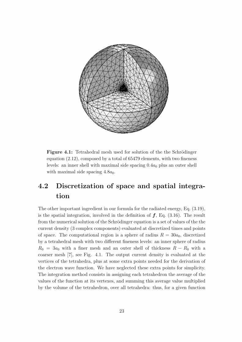
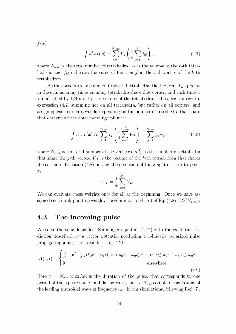
Figure 4.1: Tetrahedral mesh used for solution of the the Schrodinger

equation (2.12), composed by a total of 65479 elements, with two fineness

levels: an inner shell with maximal side spacing 0.4a0 plus an outer shell

with maximal side spacing 4.8a0.

4.2 Discretization of space and spatial integra-

tion

The other important ingredient in our formula for the radiated energy, Eq. (3.19),

is the spatial integration, involved in the definition of f , Eq. (3.16). The result

from the numerical solution of the Schrodinger equation is a set of values of the the

current density (3 complex components) evaluated at discretized times and points

of space. The computational region is a sphere of radius R = 30a0, discretized

by a tetrahedral mesh with two different fineness levels: an inner sphere of radius

R0 = 3a0 with a finer mesh and an outer shell of thickness R − R0 with a

coarser mesh [7], see Fig. 4.1. The output current density is evaluated at the

vertices of the tetrahedra, plus at some extra points needed for the derivation of

the electron wave function. We have neglected these extra points for simplicity.

The integration method consists in assigning each tetrahedron the average of the

values of the function at its vertexes, and summing this average value multiplied

by the volume of the tetrahedron, over all tetrahedra: thus, for a given function

23

f(x) ∫d3xf(x) '

Ntetr∑h=1

Vh

(1

4

4∑l=1

fhl

), (4.7)

where Ntetr is the total number of tetrahedra, Vh is the volume of the h-th tetra-

hedron, and fhl indicates the value of function f at the l-th vertex of the h-th

tetrahedron.

As the corners are in common to several tetrahedra, the the term fhl appears

in the sum as many times as many tetrahedra share that corner, and each time it

is multiplied by 1/4 and by the volume of the tetrahedron: thus, we can rewrite

expression (4.7) summing not on all tetrahedra, but rather on all corners, and

assigning each corner a weight depending on the number of tetrahedra that share

that corner and the corresponding volumes:

∫d3xf(x) ≈

Nvert∑j=1

fj

1

4

n(j)tetr∑k=1

Vjk

=Nvert∑j=1

fjwj , (4.8)

where Nvert is the total number of the vertexes, n(j)tetr is the number of tetrahedra

that share the j-th vertex, Vjk is the volume of the k-th tetrahedron that shares

the corner j. Equation (4.8) implies the definition of the weight of the j-th point

as

wj :=1

4

n(j)tetr∑k=1

Vjk .

We can evaluate these weights once for all at the beginning. Once we have as-

signed each mesh-point its weight, the computational cost of Eq. (4.8) is O(Nvert).

4.3 The incoming pulse

We solve the time-dependent Scrodinger equation (2.12) with the excitation ra-

diation described by a vector potential producing a x-linearly polarized pulse

propagating along the z-axis (see Fig. 4.2):

A(z, t) =

E0

ω0sin2

[πω0τ

(k0z − ω0t)]

sin(k0z − ω0t)x for 0 ≤ k0z − ω0t ≤ ω0τ

0 elsewhere.

(4.9)

Here τ = Nosc × 2π/ω0 is the duration of the pulse, that corresponds to one

period of the squared-sine modulating wave, and to Nosc complete oscillations of

the leading sinusoidal wave at frequency ω0. In our simulations, following Ref. [7],

24

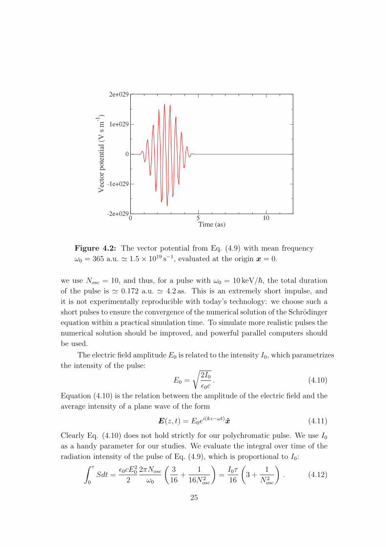
Figure 4.2: The vector potential from Eq. (4.9) with mean frequency

ω0 = 365 a.u. ' 1.5× 1019 s−1, evaluated at the origin x = 0.

we use Nosc = 10, and thus, for a pulse with ω0 = 10 keV/~, the total duration

of the pulse is ' 0.172 a.u. ' 4.2 as. This is an extremely short impulse, and

it is not experimentally reproducible with today’s technology: we choose such a

short pulses to ensure the convergence of the numerical solution of the Schrodinger

equation within a practical simulation time. To simulate more realistic pulses the

numerical solution should be improved, and powerful parallel computers should

be used.

The electric field amplitude E0 is related to the intensity I0, which parametrizes

the intensity of the pulse:

E0 =

√2I0

ε0c. (4.10)

Equation (4.10) is the relation between the amplitude of the electric field and the

average intensity of a plane wave of the form

E(z, t) = E0ei(kz−ωt)x (4.11)

Clearly Eq. (4.10) does not hold strictly for our polychromatic pulse. We use I0

as a handy parameter for our studies. We evaluate the integral over time of the

radiation intensity of the pulse of Eq. (4.9), which is proportional to I0:∫ τ

0

Sdt =ε0cE

20

2

2πNosc

ω0

(3

16+

1

16N2osc

)=I0τ

16

(3 +

1

N2osc

). (4.12)

25

Eq. (4.12), valid for Nosc > 1, was obtained empirically. It fits perfectly the

analytical integral obtained for Nosc = 2 and Nosc = 3. Moreover, for Nosc →∞the average intensity on one oscillation is 3I0/16, namely I0 multiplied by 3/8

(the average value of sin4) and by 1/2 (the average value of cos2). This is coherent

with what we might expect thinking that, for large Nosc, the electric field obtained

from (4.9) is ' E0 sin2[

πω0τ

(k0z − ω0t)]

cos(k0z − ω0t), and that the intensity is

proportional to |E|2.

Fixed Nosc, the two parameters on which one can act to modify the pulse

and study the dependence of the cross section are its intensity I0 and the photon

mean energy E0 = ~ω0. For convenience, in the numerical implementation we

adopt the atomic units (e = ~ = me = 4πε0 = 1, see Appendix A. We can rewrite

Eq. (4.10) in these units:

E0 =√

8παI0 , (4.13)

where α is the fine-structure constant. From now on we will refer to I0 in atomic

units: to convert it to the SI one can multiply it by the atomic intensity unitEHa

t0a20' 6.436× 1019 W/m2.

4.4 Convergence

We first compute the DFT of the function J(x′j, tm), obtaining the set of values

J jn := J(x′j, ωn). This calculation has a cost Nvert × N log2N . The main com-

putational effort comes now when we compute the emitted radiation. Chosen a

direction n, the discrete version of Eq. (3.19), including the explicit expression

for f in Eq. (3.20), is

dEdΩ

(n) =Z0

32π2

∆t

N

N/2−1∑n=−N/2

(ωnc

)2

∣∣∣∣∣n×Nvert∑j=1

wjJ jneikn·x′

j

∣∣∣∣∣2

. (4.14)

It is clear that this formula has a computational cost of order O(N×Nvert): if we

want to calculate the radiated energy in Ndir different directions, the total cost

becomes O(N ×Nvert ×Ndir).

We now analyse the sources of error of our study. As we make no approx-

imation in the theory (apart from the far-filed approximation, which however is

completely realized experimentally and thus introduces a negligible error, and

the classical treatment of electromagnetic fields), the only approximation of this

method arises when passing from the continuous formula (3.19) to the discretized

formula (4.14). Thus, when calculating the differential cross section we have

two sources of error: the finite discrete time sampling and the spatial discretiza-

tion. Moreover, when we want to calculate the total cross section we need to

26

approximate the integral in Eq. (3.22) with a finite sum over finite elements

∆Ω = sin θ∆θ∆φ. This fact introduces a third source of error that we will refer

to as finite angular resolution. Note that this third source of error can be eas-

ily reduced at will, as Eq. (4.14) poses no limit to the number of directions at

which one computes the radiation: it is just a question on how much computer

time one is willing spend. As the calculations for different directions are totally

independent from one another, the computation can be completely parallelized.

In the present study of convergence we set up a simulation for an incoming

pulse of intensity I0 = 106 a.u. ' 6.4× 1025 W m−2 and mean energy 365 a.u. '10 keV (see Sect. 4.3). Figures 4.3, 4.4 and 4.5 report the analysis of convergence

of our method as a function of several parameters. The time-stepping is reported

in units of the period of the leading wave τ0 = 2π/ω0: we adapt the choice of

the sampling time to the frequency of the pulse in order to keep the ratio ∆t/τ0

constant. For the studies in the following sections we adopted the following

default parameters, indicated by the arrows in the figures:

• time-step ∆t/τ0 = 0.365/π ' 0.116,

• maximal mesh spacing in the finest region 0.4a0,

• angular resolution (for the total cross section) ∆θ = ∆φ = 3.

With this choice of the parameters, our main sources of error are expected to be

the spatial mesh and the angular resolution, and we estimate our numerical error

on the total cross section to be of the order ∆σ = 0.2 mb.

27

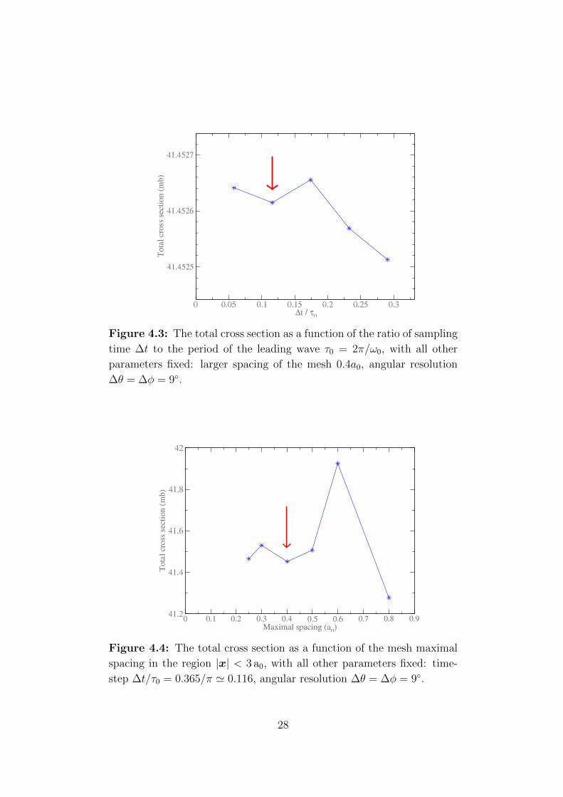
Figure 4.3: The total cross section as a function of the ratio of sampling

time ∆t to the period of the leading wave τ0 = 2π/ω0, with all other

parameters fixed: larger spacing of the mesh 0.4a0, angular resolution

∆θ = ∆φ = 9.

Figure 4.4: The total cross section as a function of the mesh maximal

spacing in the region |x| < 3 a0, with all other parameters fixed: time-

step ∆t/τ0 = 0.365/π ' 0.116, angular resolution ∆θ = ∆φ = 9.

28

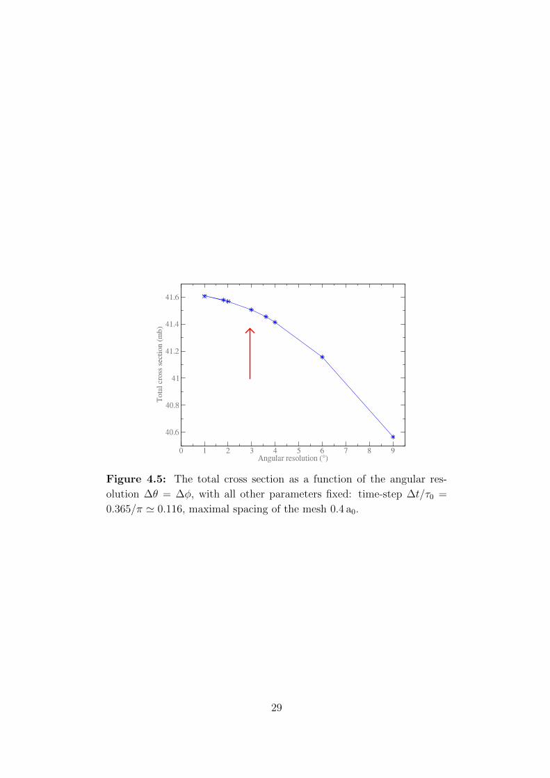
Figure 4.5: The total cross section as a function of the angular res-

olution ∆θ = ∆φ, with all other parameters fixed: time-step ∆t/τ0 =

0.365/π ' 0.116, maximal spacing of the mesh 0.4 a0.

29

Chapter 5

Results

5.1 The perturbative limit

We first test our code with a relatively moderate-intensity pulse, I0 = 104 a.u.,

for which we expect, following Ref. [7], the perturbative result to hold. The

cross section (2.20) does not consider the incoherent (Compton) scattering: we

compare our results to this formula, as, due to our classical treatment of the

electromagnetic fields, we can not predict quantum effects such as the Compton

scattering. Inelastic scattering plays a dominant role in low-Z atoms: in particular

for the hydrogen atom the total inelastic cross section at 10 keV is σC ' 0.64 bσT (see Sec. 2.2) and thus Compton is the dominant effect. However, for large

atoms or molecules, which are the main target of experimental interest, inelastic

scattering is comparably smaller, and thus for those objects our method will be

more accurate.

The fact that our method does not count for incoherent scattering is shown

also by a Fourier analysis of the scattered radiation (See Fig. 5.1): for increasing

θ some non-elastic components of the scattered radiation are observed, but they

are significantly smaller than the elastic peaks.

To illustrate how the photon energy affects the angular dependence of the

cross section, we set up two simulations with a different mean energy ~ω1 =

365 a.u. ' 10 keV and ~ω2 = 36.5 a.u. ' 1keV. Figure 5.2 reports the results

of our calculations compared with the perturbative result (2.20) for x-linearly

polarized monochromatic radiation, as our vector potential of Eq. (4.9) is: we

plot the angular dependence of the differential cross section as a function of θ,

for φ = 0 (polarization plane) and φ = 90 (perpendicular to the polarization).

30

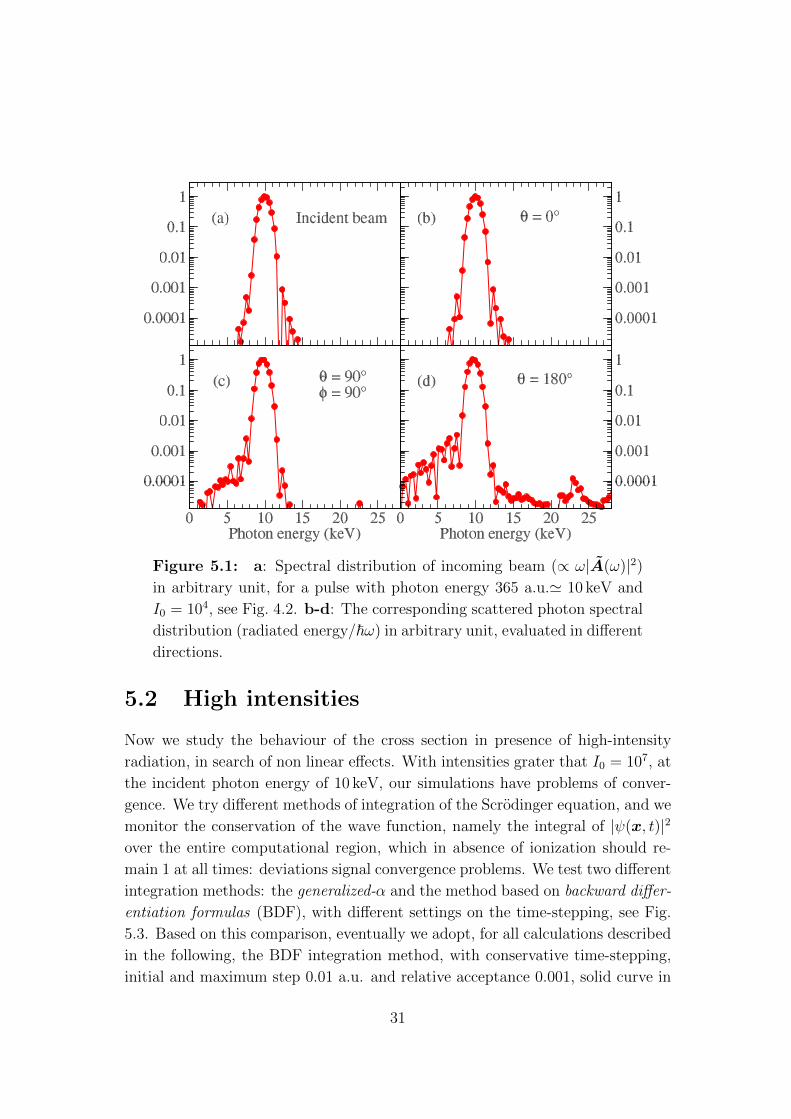
Figure 5.1: a: Spectral distribution of incoming beam (∝ ω|A(ω)|2)

in arbitrary unit, for a pulse with photon energy 365 a.u.' 10 keV and

I0 = 104, see Fig. 4.2. b-d: The corresponding scattered photon spectral

distribution (radiated energy/~ω) in arbitrary unit, evaluated in different

directions.

5.2 High intensities

Now we study the behaviour of the cross section in presence of high-intensity

radiation, in search of non linear effects. With intensities grater that I0 = 107, at

the incident photon energy of 10 keV, our simulations have problems of conver-

gence. We try different methods of integration of the Scrodinger equation, and we

monitor the conservation of the wave function, namely the integral of |ψ(x, t)|2

over the entire computational region, which in absence of ionization should re-

main 1 at all times: deviations signal convergence problems. We test two different

integration methods: the generalized-α and the method based on backward differ-

entiation formulas (BDF), with different settings on the time-stepping, see Fig.

5.3. Based on this comparison, eventually we adopt, for all calculations described

in the following, the BDF integration method, with conservative time-stepping,

initial and maximum step 0.01 a.u. and relative acceptance 0.001, solid curve in

31

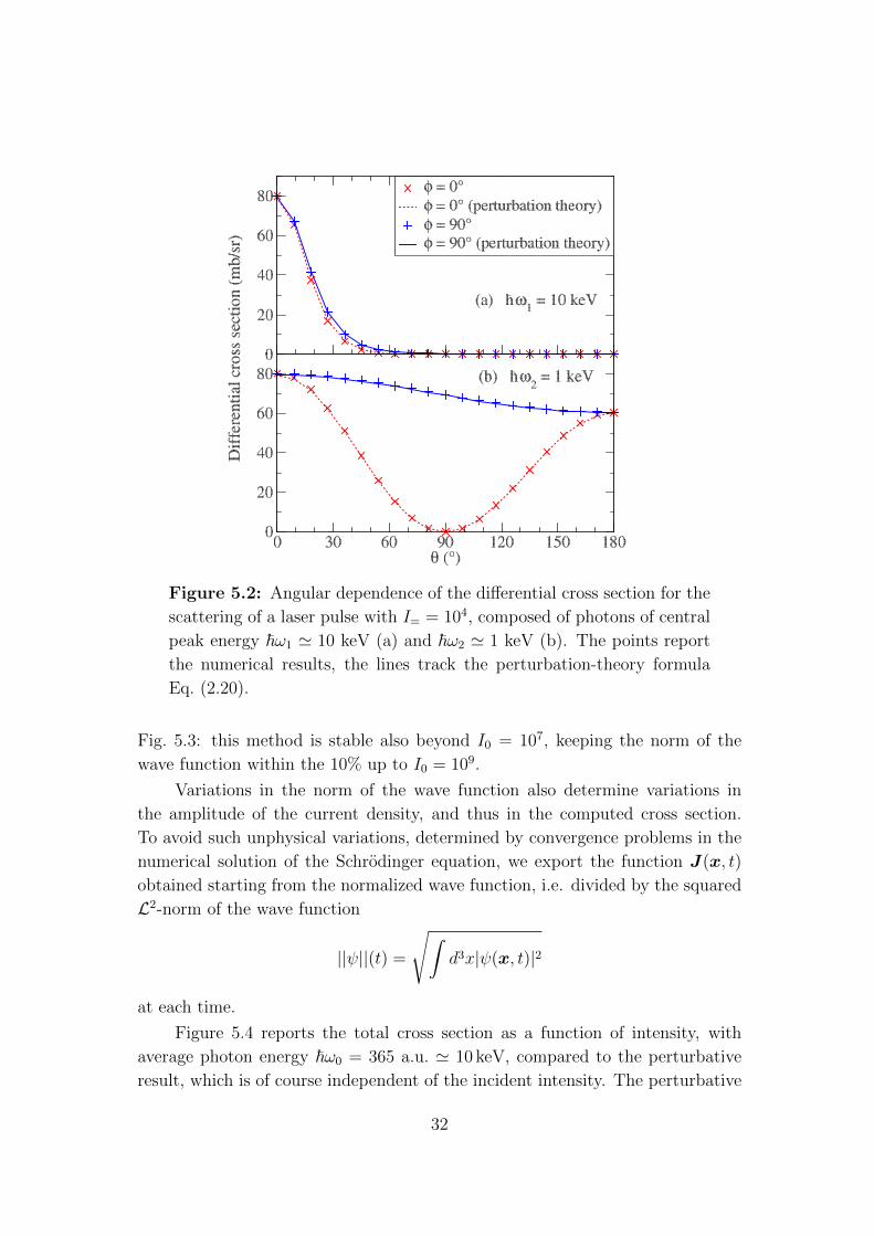
Figure 5.2: Angular dependence of the differential cross section for the

scattering of a laser pulse with I= = 104, composed of photons of central

peak energy ~ω1 ' 10 keV (a) and ~ω2 ' 1 keV (b). The points report

the numerical results, the lines track the perturbation-theory formula

Eq. (2.20).

Fig. 5.3: this method is stable also beyond I0 = 107, keeping the norm of the

wave function within the 10% up to I0 = 109.

Variations in the norm of the wave function also determine variations in

the amplitude of the current density, and thus in the computed cross section.

To avoid such unphysical variations, determined by convergence problems in the

numerical solution of the Schrodinger equation, we export the function J(x, t)

obtained starting from the normalized wave function, i.e. divided by the squared

L2-norm of the wave function

||ψ||(t) =

√∫d3x|ψ(x, t)|2

at each time.

Figure 5.4 reports the total cross section as a function of intensity, with

average photon energy ~ω0 = 365 a.u. ' 10 keV, compared to the perturbative

result, which is of course independent of the incident intensity. The perturbative

32

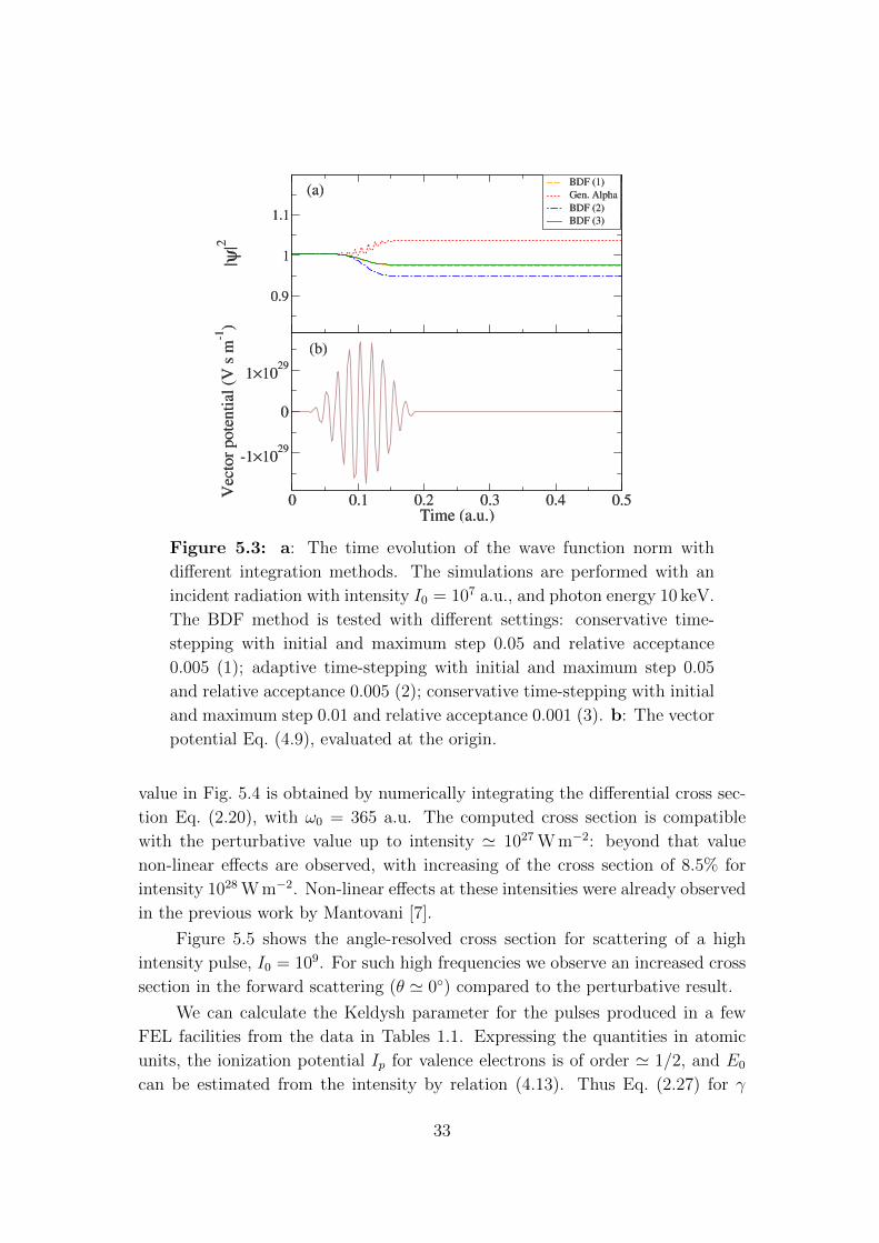
Figure 5.3: a: The time evolution of the wave function norm with

different integration methods. The simulations are performed with an

incident radiation with intensity I0 = 107 a.u., and photon energy 10 keV.

The BDF method is tested with different settings: conservative time-

stepping with initial and maximum step 0.05 and relative acceptance

0.005 (1); adaptive time-stepping with initial and maximum step 0.05

and relative acceptance 0.005 (2); conservative time-stepping with initial

and maximum step 0.01 and relative acceptance 0.001 (3). b: The vector

potential Eq. (4.9), evaluated at the origin.

value in Fig. 5.4 is obtained by numerically integrating the differential cross sec-

tion Eq. (2.20), with ω0 = 365 a.u. The computed cross section is compatible

with the perturbative value up to intensity ' 1027 W m−2: beyond that value

non-linear effects are observed, with increasing of the cross section of 8.5% for

intensity 1028 W m−2. Non-linear effects at these intensities were already observed

in the previous work by Mantovani [7].

Figure 5.5 shows the angle-resolved cross section for scattering of a high

intensity pulse, I0 = 109. For such high frequencies we observe an increased cross

section in the forward scattering (θ ' 0) compared to the perturbative result.

We can calculate the Keldysh parameter for the pulses produced in a few

FEL facilities from the data in Tables 1.1. Expressing the quantities in atomic

units, the ionization potential Ip for valence electrons is of order ' 1/2, and E0

can be estimated from the intensity by relation (4.13). Thus Eq. (2.27) for γ

33

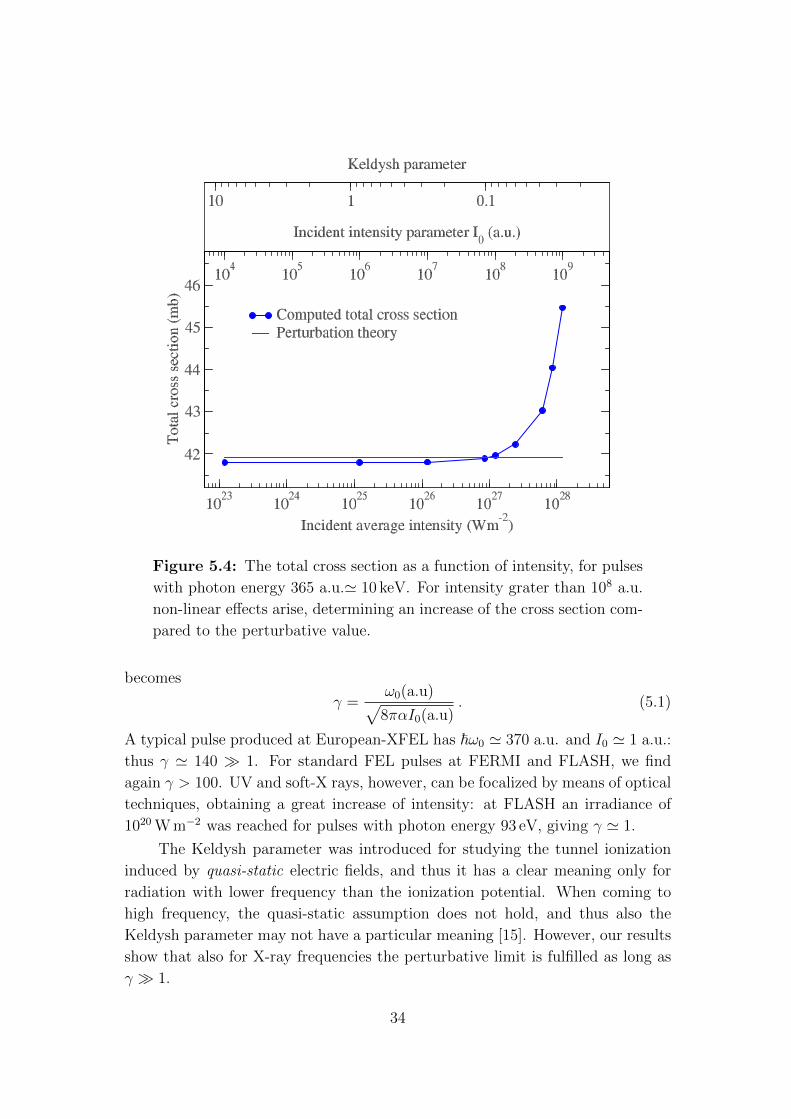
Figure 5.4: The total cross section as a function of intensity, for pulses

with photon energy 365 a.u.' 10 keV. For intensity grater than 108 a.u.

non-linear effects arise, determining an increase of the cross section com-

pared to the perturbative value.

becomes

γ =ω0(a.u)√8παI0(a.u)

. (5.1)

A typical pulse produced at European-XFEL has ~ω0 ' 370 a.u. and I0 ' 1 a.u.:

thus γ ' 140 1. For standard FEL pulses at FERMI and FLASH, we find

again γ > 100. UV and soft-X rays, however, can be focalized by means of optical

techniques, obtaining a great increase of intensity: at FLASH an irradiance of

1020 W m−2 was reached for pulses with photon energy 93 eV, giving γ ' 1.

The Keldysh parameter was introduced for studying the tunnel ionization

induced by quasi-static electric fields, and thus it has a clear meaning only for

radiation with lower frequency than the ionization potential. When coming to

high frequency, the quasi-static assumption does not hold, and thus also the

Keldysh parameter may not have a particular meaning [15]. However, our results

show that also for X-ray frequencies the perturbative limit is fulfilled as long as

γ 1.

34

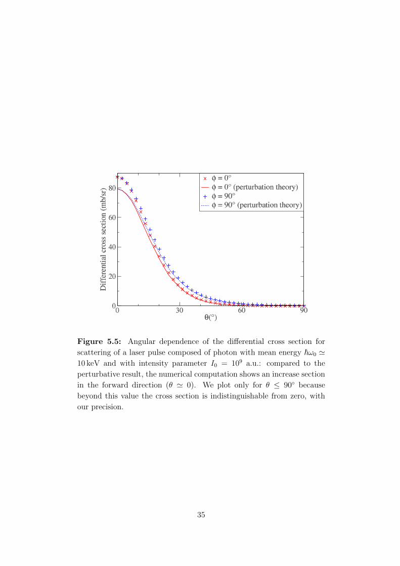
Figure 5.5: Angular dependence of the differential cross section for

scattering of a laser pulse composed of photon with mean energy ~ω0 '10 keV and with intensity parameter I0 = 109 a.u.: compared to the

perturbative result, the numerical computation shows an increase section

in the forward direction (θ ' 0). We plot only for θ ≤ 90 because

beyond this value the cross section is indistinguishable from zero, with

our precision.

35

Chapter 6

Conclusions and outlooks

In the present thesis we have reached a further step in the Maxwell-Schrodinger

approach to X-ray radiation started with the work [7]. In particular we offer

theoretical basis and numerical implementation to the problem of predicting the

far-field scattering cross section, given the time-dependent current density dis-

tribution obtained from a solution of the Maxwell-Schrodinger problem. The

code we provide has a computational cost which is proportional to the number

of points that form the spatial mesh, times the number of steps in which the

simulation time is divided, times the number of directions in which the outgoing

radiation is computed. An important feature of our code is that the calculations

in different directions are completely independent from one another, and thus the

computation can in principle be completely parallelized. We tested the code in

several pulse conditions, proving that, for low intensities, our predictions are in

complete accordance with the analytical result coming from perturbative meth-

ods. The code can be applied to any case of scattering, not only from one-electron

atoms, provided that we solve the many-body Schrodinger equation and extract

the global current density function from it, taking into account the motion of all

electrons.

An extension of the model may come from including, in the Schrodinger

equation, the electromagnetic field generated by the electronic motion itself, thus

solving a system of coupled equations, with the Schrodinger equation solved along-

side the equations of the Maxwell potentials, now treated as variables too. This

would also implement the energy loss of the electron, which after the excitation

falls back into its ground state by emitting energy which is transformed into

electromagnetic radiation.

The model may be generalized for heavier atoms and molecules, by imple-

menting a many-body Schrodinger equation. Heavy molecules, which are the

main source of interest for experimental applications, may also fit better in this

36

approach, as the Compton scattering, which we do not take into account due

to the classical treatment of electromagnetic fields, may be smaller than in light

atoms.

Improvements should be made particularly in the numerical solution of the

Schrodinger equation. In particular, the convergence of the algorithm should be

enhanced to make it possible to simulate longer pulses, of the order of the fs,

which is the typical time scale of FEL pulses.

37

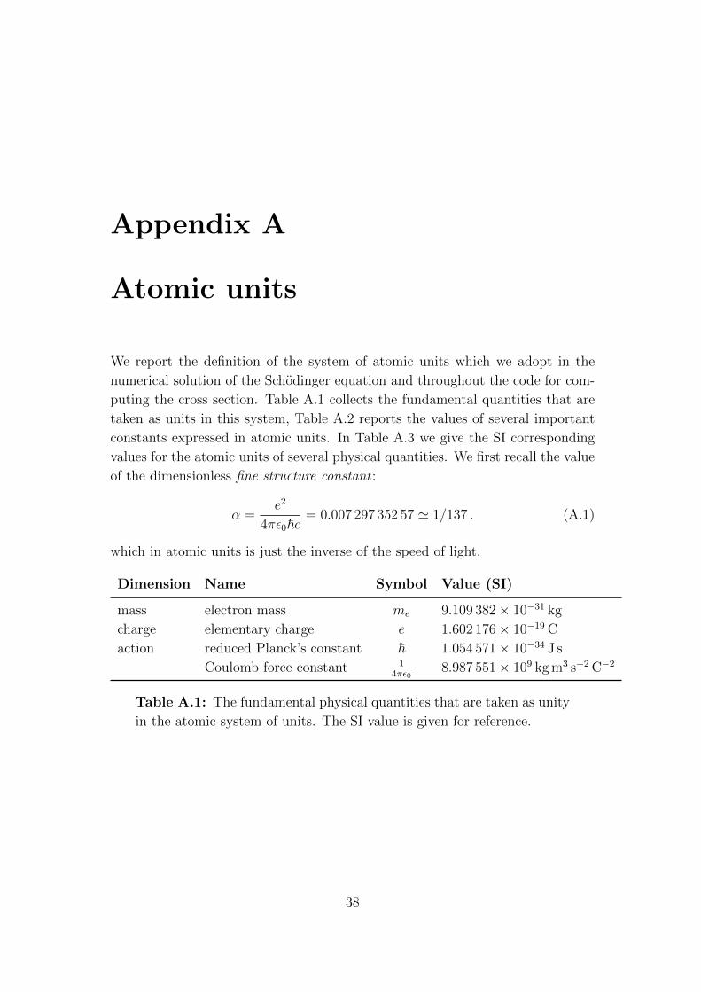
Appendix A

Atomic units

We report the definition of the system of atomic units which we adopt in the

numerical solution of the Schodinger equation and throughout the code for com-

puting the cross section. Table A.1 collects the fundamental quantities that are

taken as units in this system, Table A.2 reports the values of several important

constants expressed in atomic units. In Table A.3 we give the SI corresponding

values for the atomic units of several physical quantities. We first recall the value

of the dimensionless fine structure constant :

α =e2

4πε0~c= 0.007 297 352 57 ' 1/137 . (A.1)

which in atomic units is just the inverse of the speed of light.

Dimension Name Symbol Value (SI)

mass electron mass me 9.109 382× 10−31 kg

charge elementary charge e 1.602 176× 10−19 C

action reduced Planck’s constant ~ 1.054 571× 10−34 J s

Coulomb force constant 14πε0

8.987 551× 109 kg m3 s−2 C−2

Table A.1: The fundamental physical quantities that are taken as unity

in the atomic system of units. The SI value is given for reference.

38

Constant Symbol Value (a.u.) Value (SI)

speed of light c α−1 = 137.036 299 792 458 m s−1

vacuum permittivity ε01

4π= 0.079 577 8.854 188× 10−12 F m−1

vacuum permeability µ0 4πα2 = 6.691 762× 10−4 4π × 10−7 V s A−1 m−1

classical electron radius re 5.325 135× 10−5 2.817 940× 10−15 m

Bohr magneton µB 0.5 9.274 009× 10−24 J T−1

Table A.2: A few physical constants used in the present thesis, ex-

pressed in atomic units, and in the SI.

Dimension Name Symbol Expression Value (SI)

length Bohr

radius

a04πε0~2mee2

5.291 771× 10−11 m

energy Hartree

energy

EHae2

4πεa04.359 744× 10−18 J

time t0~

EHa2.418 884× 10−17 s

frequency t0−1 4.134 138× 1016 s−1

angular frequency 2πt0

2.597 555× 1017 s−1

power EHat0

0.180 237 8 W

electric current density et0a20

2.365 337× 1018 A m−2

electric field EHaea0

5.142 207× 1011 V m−1

electric potential EHae 27.211 385 V

magnetic induction ~ea20

2.350 517× 105 T

vector potential ~ea0

1.243 840× 10−5 V s m−1

energy flux (intensity) EHa

t0a206.436 409× 1019 W m−2

magnetic permeability mea0e2

1.8779× 10−3 V s A−1 m−1

Table A.3: Derived atomic units for the physical quantities appearing

in the present work, with their SI value.

39

Ringraziamenti

Ringrazio di cuore il professor Manini, per la disponibilita che mi ha mostrato

ogni volta che avevo bisogno e per i dialoghi costruttivi che ho avuto con lui, in

cui ho imparato molte cose, ma soprattuto ho imparato che spesso le cose sono

assai piu complesse di quello che penso. Ringrazio il professor Onida, al quale

devo la possibilita di intraprendere questo lavoro. Voglio ringraziare molto anche

Mattia, che pur nel pieno del suo dottorato a Konstanz e sempre stato disponibile

a rispondere alle mie domande, con pazienza e chiarezza.

In secondo luogo, voglio ringraziare la mia famiglia per il sotegno che mi ha

sempre garantito in questi anni.

Un sentito grazie va a tutti gli amici che in questi anni hanno condiviso con

me un pezzo di strada. Tra i nomi che voglio ricordare c’e certamente quello

di Nigel, il mio piu longevo compagno di studi, per la sua amicizia che e un

vero dono. Ringrazio il nonno Luca, perche nonostante tutto rimane fedele alla

sua missione di credere in me, e perche e una persona che sa capire quando

hai bisogno che ti si offra un caffe: sarebbe stato bello festeggiare insieme oggi!

Grazie a tutti gli amici fisici: quelli del mio anno, con cui ho condiviso la vita

e lo studio quotidiano, e anche tutti gli altri della comunita che sono troppi per

essere nominati tutti ma spero si sentano ringraziati tutti, singolarmente. Un

grazie speciale alla Betta, per tutto quello che e stata per me, in questi mesi e

non solo. Poi devo per forza citare gli amici del CdB, ai quali devo il mio ingresso

nel mondo del gioco, dell’alcool, e dei film ignoranti. Ringrazio Skizzo, Marta

Casti, Franci Geno, Mona, e tutti gli amici che vedo meno spesso, anche per

colpa mia. Ringrazio tutti gli amici dell’alecrim, perche in questi anni quel luogo

e stato sempre un punto fermo. Ringrazio i quattro ”primulini” (piu uno) e tutti

gli amici con cui ho condiviso l’amore per il canto e la musica.

Ringrazio il Signore per tutto questo che mi ha donato, chiedendogli di farmi

vedere che strada ha preparato per me.

40

Bibliography

[1] A. Thompson et al., X-ray Data Booklet, Sec. 2.2, Lawrence Berkeley Na-

tional Laboratory (2009). URL: http://xdb.lbl.gov.

[2] K. J. Gaffney, H. N. Chapman, Imaging atomic structure and dynamics with

ultrafast X-ray scattering, Science 316, 1444 (2007).

[3] G. Dixit, J. M. Slowik, R. Santra, Theory of time-resolved nonresonant X-

ray scattering for imaging ultrafast coherent electron motion, Phys. Rev. A

89, 043409 (2014).

[4] L. V. Keldysh, Ionization in the field of a strong electromagnetic wave, Soviet

Physics JETP 20, 1307 (1965).

[5] A. Fratalocchi, G. Ruocco, Single-molecule imaging with X-ray free-electron

lasers: dream or reality?, Phys. Rev. Lett. 106, 105504 (2011).

[6] A. Fratalocchi, C. Conti, G. Ruocco, F. Sette, Nonlinear refraction of hard

X-rays, Phys. Rev. B 77, 245132 (2008).

[7] M. Mantovani, Ultrafast X-ray scattering beyond linear-response theory,

diploma thesis (University Milan, 2016), http://materia.fisica.unimi.

it/manini/theses/mantovani.pdf.

[8] J. D. Jackson, Classical Electrodynamics (Wiley, USA, 1998).

[9] J. H. Hubbell, W. J. Veigele, E. A. Briggs, R. T. Brown, D. T. cromer, R. J.

Howerton, Atomic form factors, incoherent scattering functions, and photon

scattering cross sections, J. Phys. Chem. Ref. Data 4, 471 (1975).

[10] T. W. Korner, Fourier Analysis (Cambridge Univ. Press, Cambridge, 1989).

[11] N. Fusco, P. Marcellini and C. Sbordone, Analisi Matematica Due (Liguori,

Napoli, 1996).

41

[12] E. C. Titchmarsh, Introduction to the theory of Fourier Integrals (Oxford

Univ. Press, Oxford, 1948).

[13] W. H. Press, S. A. Teukolsky, W. T. Vetterling and B. P. Flannery, Numerical

Recipes in C++: the art of scientific computing (Cambridge Univ. Press,

Cambridge, 2002).

[14] FFTW library, http://fftw.org/.

[15] H. R. Reiss, Unsuitability of the Keldysh parameter for laser fields, Phys.

Rev. A 82, 023418 (2010).

42