1

Angular Power Distribution and Mean Effective Gain of MobileAntenna in Different Propagation Environments

Kimmo Kalliola1, Kati Sulonen2, Heikki Laitinen3, Outi Kivekäs2, Joonas Krogerus1,Pertti Vainikainen2, Member, IEEE

1Nokia Research Center, Radio Communications Laboratory2Helsinki University of Technology, Radio Laboratory

3VTT Information Technology

Abstract −−−− We measured the elevation angle distribution and cross-polarization power ratio of the

incident power at the mobile station in different radio propagation environments at 2.15 GHz frequency.

A novel measurement technique was utilized, based on a wideband channel sounder and a spherical dual-

polarized antenna array at the receiver. Data was collected along over 9 km of continuous measurement

routes, both indoor and outdoor. Our results show that in NLOS situations the power distribution in

elevation has a shape of a double-sided exponential function, with different slopes on the negative and

positive sides of the peak. The slopes and the peak elevation angle depend on the environment and base

station antenna height. The cross-polarization power ratio varied within 6.6 and 11.4 dB, being lowest for

indoor, and highest for urban microcell environments. We applied the experimental data for analysis of

the mean effective gain (MEG) of several mobile handset antenna configurations, with and without user’s

head. The obtained MEG values varied from approximately −−−−5 dBi in free space to less than −−−−11 dBi

beside the head model. These values are considerably lower than what is typically used in system

specifications. The result shows that considering only the maximum gain or total efficiency of the antenna

is not enough to describe its performance in practical operating conditions. For most antennas the

environment type has little effect on the MEG, but clear differences exist between antennas. The effect of

user’s head on the MEG depends on the antenna type, and on which side of the head the user holds the

handset.

I. INTRODUCTION

The gain of a mobile handset antenna is a critical parameter in cellular network design. Due to the large variety

of mobile phones used in the networks, it is very important that their antenna performance can be evaluated

reliably. The traditional definition of antenna gain is not adequate for evaluating the performance of a handset

antenna, whose orientation relative to the direction and polarization of the incident field is unknown. Several

2

methods have been proposed for determining the performance of a mobile antenna in realistic propagation

conditions.

The random-field measurement (RFM) method [1-4] is based on measuring the mean received power level of the

antenna on a random route in a typical operating environment. The mean effective gain (MEG) of the antenna is

obtained as the ratio of the mean signal levels of the test antenna and a reference antenna. The effect of the user

holding the handset on the antenna gain can be easily analyzed with this method [5,6]. The method is naturally

closest to realism, but it is time consuming, since the repeatability of the measurements is poor, and statistical

significance can only be achieved by doing extensive measurements in all possible operating environments. The

RFM method can be simplified by using a field simulator to produce an artificial scattering environment in an

indoor facility [7,8]. This makes the measurements repeatable, but it is not evident that the conditions resemble a

realistic operating environment.

In [9], Taga derived a general expression for MEG. Using the formulas presented in [9], the MEG of an antenna

in a certain environment can be computed based on the 3-D gain pattern of the antenna and the average angular

distribution of incident power in the environment. The power distribution must be known in both azimuth and

elevation, and separately for horizontally (φ-) and vertically (θ-) polarized field components. Also the cross-

polarization power ratio (XPR) is needed in the calculation.

The clear benefit of the computational method for determining the MEG is that it is fast and repeatable. In

addition to [9], it has been used in [4,5,10]. Currently the drawback is that there is little information available of

realistic field distributions in different environments. From the random orientation of the mobile antenna in

azimuth it is straightforward to assume that the azimuth distribution of the waves is uniform. Instead, no

straightforward assumption can be justified for the distribution in elevation. Few published results exist on

measured elevation power distributions [9,11,12]. Only [9] proposes a parameterized model for the distribution

and gives the model parameters fitted to experimental data at 900 MHz, but is limited to urban macrocell

environment with large base station antenna height. Another model was proposed in [13], but no measurement

data was given to verify or tune the model.

In this contribution we present experimental results of the elevation power distribution (EPD) and XPR at the

mobile antenna in different radio environments at 2.15 GHz frequency. The measurements were performed using

a wideband radio channel sounder and a spherical dual-polarized antenna array. The measurement method,

3

described in [14], enables the full 3-D measurement of the spatial radio channel in real time, and thus the

acquisition of large amounts of data. We compare two parameterized models for the EPD: the symmetrical

Gaussian function proposed by Taga [9], and the asymmetrical general double-exponential function. We also

present the fitted parameter values of both models for each measurement environment.

In addition, we apply the experimental results for MEG calculations of several practical mobile antenna

configurations, with both measured and simulated radiation patterns. We consider the dependence of the MEG

on the usage environment, and compare the MEG of a handset antenna to the total efficiency, gain, and cross-

polarization discrimination of the antenna configuration. Furthermore, we investigate the deviation of the MEG

values caused by using the model EPDs instead of the measured.

II. MEAN EFFECTIVE GAIN

According to Taga [9], the MEG of an antenna can be expressed using the 3-D power gain pattern of the antenna

and the angular power density functions of radio waves in a multipath environment, both defined separately for

the θ- and φ-polarized1 field components. Also the cross-polarization power ratio, i.e. the ratio of the mean

incident θ- and φ-polarized powers along a random route in the case of θ-polarized transmission [9], is needed in

the computation of MEG. The angular power density functions ( )φθ ,θp and ( )φθ ,φp need to satisfy the

following condition:

( ) ( ) 1cos,cos,2

0

2/

2/

2

0

2/

2/θ == ∫ ∫∫ ∫

−φ

−

φθθφθφθθφθπ π

π

π π

π

ddpddp (1)

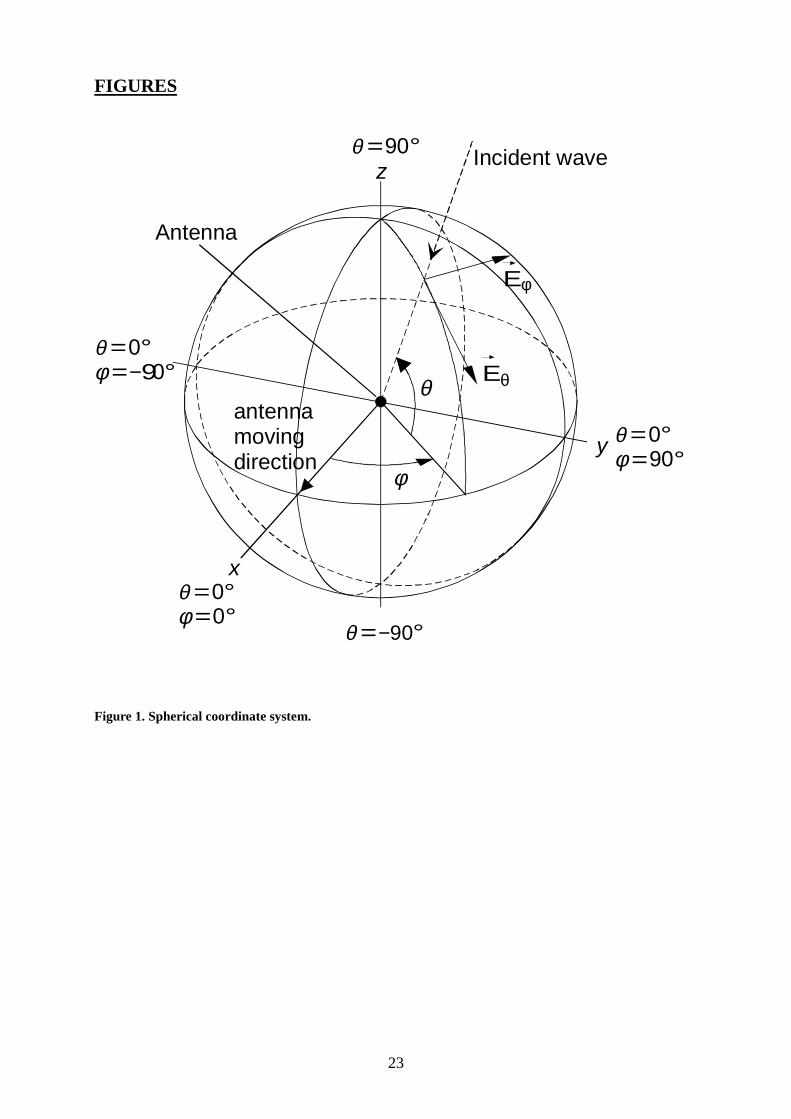
The spherical coordinate system is defined in Fig. 1. It should be noted that according to (1) the definition of the

angular power density functions differs from that of the joint probability density function for the direction of

arrival ( )φθ ,f , defined in [15], which satisfies:

( ) 1,2

0

2/

2/

=∫ ∫−

φθφθπ π

π

ddf (2)

1 θ and φ polarizations correspond to the vertical and horizontal polarizations used in [9] in the planeperpendicular to the incidence angle

4

It follows by combining (1) and (2) that the relation between the angular power density function and joint

probability density function for the direction of arrival is:

( ) ( )θφθφθ

cos,, fp = (3)

It is natural to assume that when a mobile user moves randomly in any environment, the incident waves can arise

from any azimuth direction with equal probability. If the power density function in azimuth is uniform and

independent of elevation, the joint angular power density functions reduce to:

( ) ( )θπ

φθ pp21, = (4)

In contrast to the azimuth, no straightforward assumption can be justified for the power distribution in elevation.

Previously few models have been presented. The first model by Clarke [16] assumes that all energy is

concentrated in the horizontal plane. However, it is known to be unrealistic at least in urban environments, where

buildings give rise to multipath components from high elevation angles. Aulin [17], proposed a generalization of

Clarke’s model to a case where all energy does not travel in the horizontal plane, but no data was available to

verify the model. Also reference [13], which proposes a family of functions to describe the power distribution in

elevation, lacks measurement data. In [9], Taga proposed the Gaussian density function, and fitted the

parameters to experimental data. However, he used only four measured points of the elevation power

distribution, which is not necessarily sufficient to verify the distribution.

III. DESCRIPTION OF EXPERIMENTS

A. Measurement Setup

We measured the angular power distribution separately for θ- and φ-polarized components of the incident field at

the mobile station in different propagation environments using the measurement method presented in [14]. The

method is based on a spherical array of 32 dual-polarized antenna elements, and a complex wideband radio

channel sounder. At the base station (BS), a wideband signal was transmitted using a single fixed vertically

5

polarized antenna. At the mobile station (MS), the signal was received separately from the θ- and φ-polarized

feeds of each of the 32 elements of the spherical array, using a fast 64-channel RF switch. Approximately five

snapshots2 of the received signal were sampled and stored per each wavelength the mobile moved, except for the

highway macrocell environment, where the number of snapshots per wavelength was between two and three.

The center frequency was 2.154 GHz and the carrier was modulated by a PN-sequence with 30 MHz chip

frequency. Detailed information of the used HUT/IDC channel sounder can be found in [18].

During the measurements the transmitting antenna was placed in fixed locations corresponding to typical BS

antenna installations in different cellular radio network configurations. A modified commercial GSM1800 sector

antenna with 10 dBi gain and 3 dB beamwidth of 80° in azimuth and 28° in elevation was used in all cases

except for the indoor picocell, where the transmitting antenna was omnidirectional (vertical 3 dB beamwidth

80°, gain 2 dBi). It must be noted that the radiation pattern of the transmitting antenna affects the power

distribution at the receiver. The transmitting antennas were chosen as typical examples of BS antennas used in

existing networks at cell configurations similar to the measured ones, to obtain as realistic results as possible.

B. Processing of Data

The delays, directions-of-arrival (DoAs), amplitudes, and phases of both θ- and φ-polarized components of the

incoming waves at each measurement snapshot were found through sequential delay-domain and angular-

domain processing. First the received signal of each antenna feed was correlated with a replica of the transmitted

PN-sequence to obtain the complex impulse response of the channel. The delay taps were then identified by

detecting the local maxima of the power delay profile averaged over the array elements. Corresponding to each

delay tap, there may exist one multipath component or several components separated by their DoAs. Up to four

multipath components per delay tap were estimated using the beamforming scheme with pre-computed array

weights (2° beam spacing in azimuth and elevation), as described in [14]. Only such multipaths were accepted

whose amplitude exceeded a threshold value of 6 dB below the highest multipath, in order to filter out spurious

signals due to sidelobes of the array. The measured sidelobe level of the array is approximately −10 dB in the

case of two simultaneous multipaths [14], but the level increases with an increasing number of multipaths.

2 one PN sequence period from all 64 channels

6

The amplitudes and phases of the θ- and φ-polarized components of the incident waves were obtained by

pointing θ- and φ-polarized beams in these directions. As a final result, we had for each measurement snapshot

the angle resolved impulse response, defined as:

( )( ) ( ) ( ) ( )ll

L

ll

l

,l

hh

ττδφφδθθδαα

τφθτφθ

−−−

=

∑= φφ 1 ,

θθ

,,,,

(5)

where θh and φh denote the θ- and φ-polarized components of the impulse response, respectively. l,θα and

l,φα are the complex amplitudes of lth multipath, θl and φl are the corresponding elevation and azimuth angles,

and τ l is the delay.

The total spatial resolution of the measurement is determined by the angular resolution of the spherical array of

approximately 40° and the 33 ns delay resolution of the wideband channel sounder. Thus the spatially separable

blocks are truncated cones with an opening angle of 40° and length of 10 m, and the size of the block increases

with increasing distance between the last scattering point and the array. The azimuth and elevation power

distributions for θ- and φ-polarized wave components were derived from the angle resolved impulse response

using formulas presented in Table 1. First the instantaneous power vs. incidence angle was computed as a sum of

the multipath powers. Then the mean relative power vs. incidence angle in one environment was obtained by

averaging over all snapshots in the environment. The variation of the received power due to large scale fading

was compensated by normalizing the result to the total incident power at each point. Due to the large

measurement bandwidth compared to the channel coherence bandwidth the fast fading of the total received

power (sum of the multipath powers) was small. The distribution of the square root of the total power agreed

well with Rice distribution and the average fitted Rice factor varied from k≈17 in the outdoor-indoor case to

k≈60 in the urban macrocell case. Finally the azimuth (APD) and elevation power distributions (EPD) were

obtained from the mean relative powers vs. incidence angle as presented in Table 1.

C. Measurement Environments

We performed measurements in five different radio environments. The environments, the approximate total route

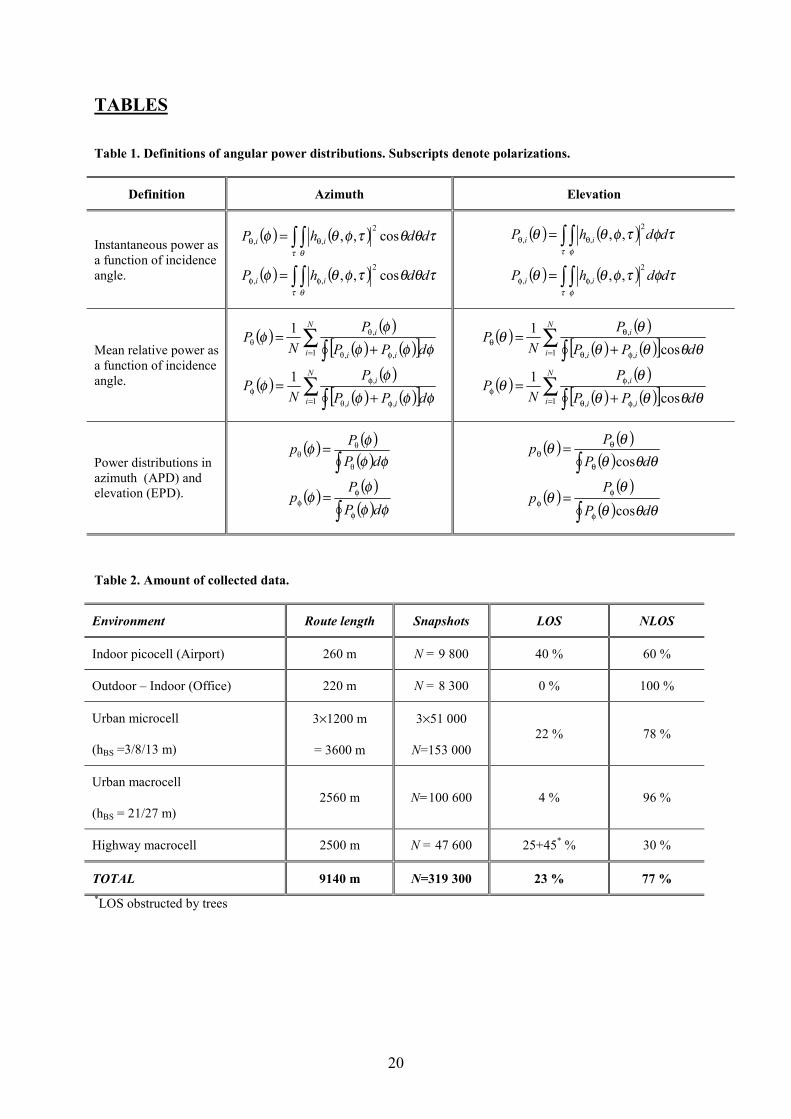
lengths, and the numbers of collected snapshots are presented in Table 2. Also the percentages of line-of-sight

(LOS) and non-line-of-sight (NLOS) measurements are shown. The characteristic features of each environment

7

are briefly described below. In all measurements except of those of the highway macrocell the spherical array

acting as the mobile station was mounted on a trolley, where the center of the array was at height of 1.7 m above

ground level and the visible arc in elevation was from zenith to approximately −60°.

The indoor picocell measurements were carried out in the transit hall of Helsinki airport. The omnidirectional BS

antenna was elevated at 4.6 m above the floor level and located so that the visibility over the hall was good. The

BS−MS distance varied from 10 to 150 m. The portion of LOS measurements was significant, of the order of 40

%.

The outdoor−indoor measurements were performed in two different office buildings, both having four floors,

and office rooms next to the outer walls made of brick. In both sites the BS antenna was placed on the rooftop of

the neighboring building. The average distance from BS to the mobile routes was in the range of 50 to 100 m.

The short distance was forced by the limited sensitivity of the measurement due to the losses in the switching

unit. The BS antenna was approximately 3 and 8 m above the mobile antenna for the two sites. The measurement

routes include both corridors and office rooms, and the ceiling height is in the range of 2.5 to 3 m in both

buildings.

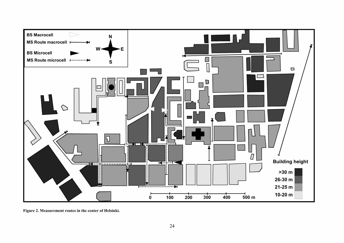
The urban micro- and macrocell measurements were performed in the center of Helsinki, Finland. The spherical

array was located on a trolley, and the routes were driven along the sidewalks of the streets. Fig. 2 presents a

map showing the BS positions and the measured mobile routes. The street grid in the measurement area is fairly

regular and the average street width is approximately 15 m. The height of most buildings is in the range of 20 to

30 m.

In the microcell environment the same mobile routes were measured for the same base station location with three

different BS antenna heights. The antenna was located on the sidewalk of a street, and mounted on a person lift

elevated at 3, 8, and 13 m above the street level. The main beam of the antenna pointed west along the street.

The measurement routes included the main street with LOS to the BS, the two parallel streets on both sides, and

four transversal streets in front of the antenna (see Fig. 2). The BS−MS distance varied from 10 to 350 m.

In the urban macrocell measurements the BS antenna was located on the rooftop of a parking house and pointed

separately to two opposite directions in order to cover larger area (see Fig. 2). The antenna heights from ground

were 27 and 21 m, the former being at, and the latter above the rooftop level of the opposite buildings.

Photographs showing the views from both macrocell antenna installations can be found in [19]. The BS−MS

8

distance varied from 50 to 750 m. Due to the limited sensitivity of the measurement system we were not able to

measure propagation distances corresponding to the radii of biggest urban macrocells. However, our

measurement distances are in line with many current urban site configurations in cellular networks today.

The highway macrocell measurements were carried out in an industrial area in Espoo, Finland. The BS antenna

was located on top of a building next to a junction of a ring road with a lot of traffic. Few large buildings exist in

the area, and for most of the routes only trees obstruct the direct LOS path. The BS antenna height was 17 m.

The measurement routes included the transversal ring road, and the crossing road. The BS−MS distance varied

from 50 to 1200 m. In these measurements the spherical array was mounted inside a person car, on the front seat,

and at the height of the passenger’s head (1.3 m). It must be noted that the metallic chassis of the car has a

significant effect on the angular distribution and polarization of the electric field at the antenna inside the car.

However, it is common nowadays to use mobile handsets inside vehicles, which makes this a practical scenario.

IV. ANGULAR DISTRIBUTION OF INCIDENT POWER

A. Experimental Azimuth Power Distribution

When a mobile antenna moves along a random route, uniform distribution is the only reasonable assumption for

the power distribution in azimuth. However, to illustrate the radio propagation in urban environment, we present

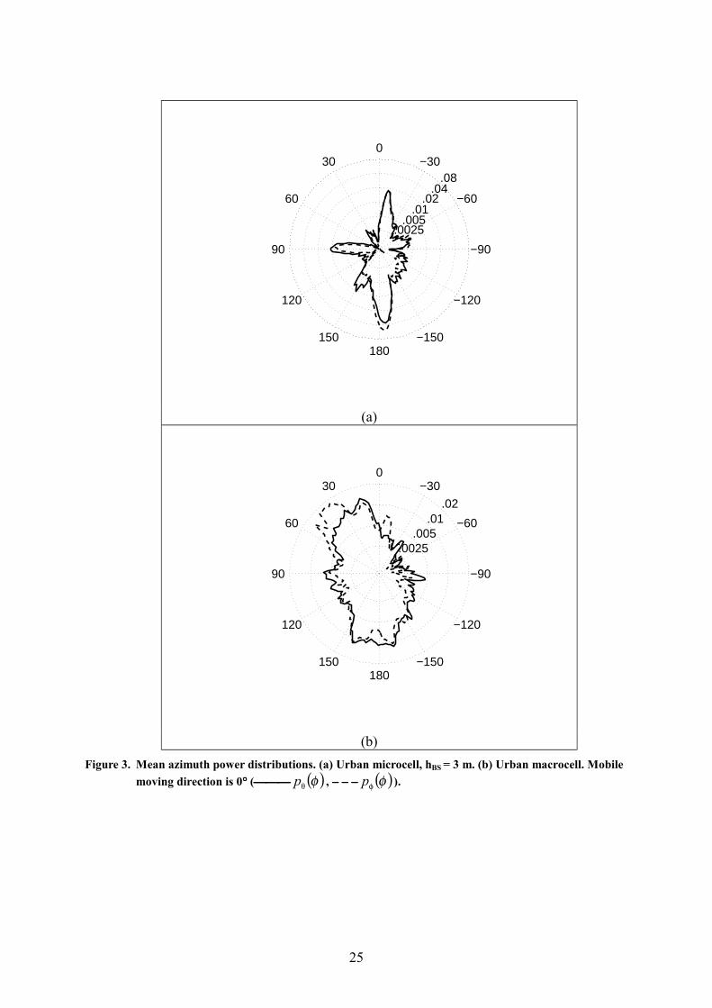
two examples of measured power distributions in different environments. Fig. 3 shows the APD in urban

microcell (hBS = 3 m) and urban macrocell environments. It can be seen that the distributions are not at all

uniform, but that some directions are more probable than others. This is due to the fact that the measured mobile

routes are not random in nature, but that they are parallel and perpendicular to street canyons (see Fig. 2). In the

microcell case, Fig. 3 (a), highest maxima are produced in directions close to 0° and 180°, i.e. the directions of

the street canyon along which the mobile is moving. The third maximum at left (90°) is due to propagation via

crossing streets. The routes were by chance chosen so that the BS is almost always at left-hand side when

looking to the moving direction of the mobile. If this had not been the case, the obtained azimuth power

distribution would have four maxima with angular separation of 90°. In the macrocell case, Fig. 3 (b), the APD

is closer to uniform than in the microcell, but the left hand side of the distribution (angles 0°...+180°) clearly

dominates. As in the microcell, the reason for this is that the routes were not random. However, since a real

mobile user may turn around or cross the streets at any angle, uniform distribution is the only justified

9

assumption for the azimuth power distribution averaged over a random route in any environment. Fig. 3 shows

that both in urban micro- and macrocell cases the differences between the θ- and φ-polarized distributions are

small.

B. Experimental Elevation Power Distribution

In contrast to the azimuth, it seems obvious that the elevation power distribution depends on the environment

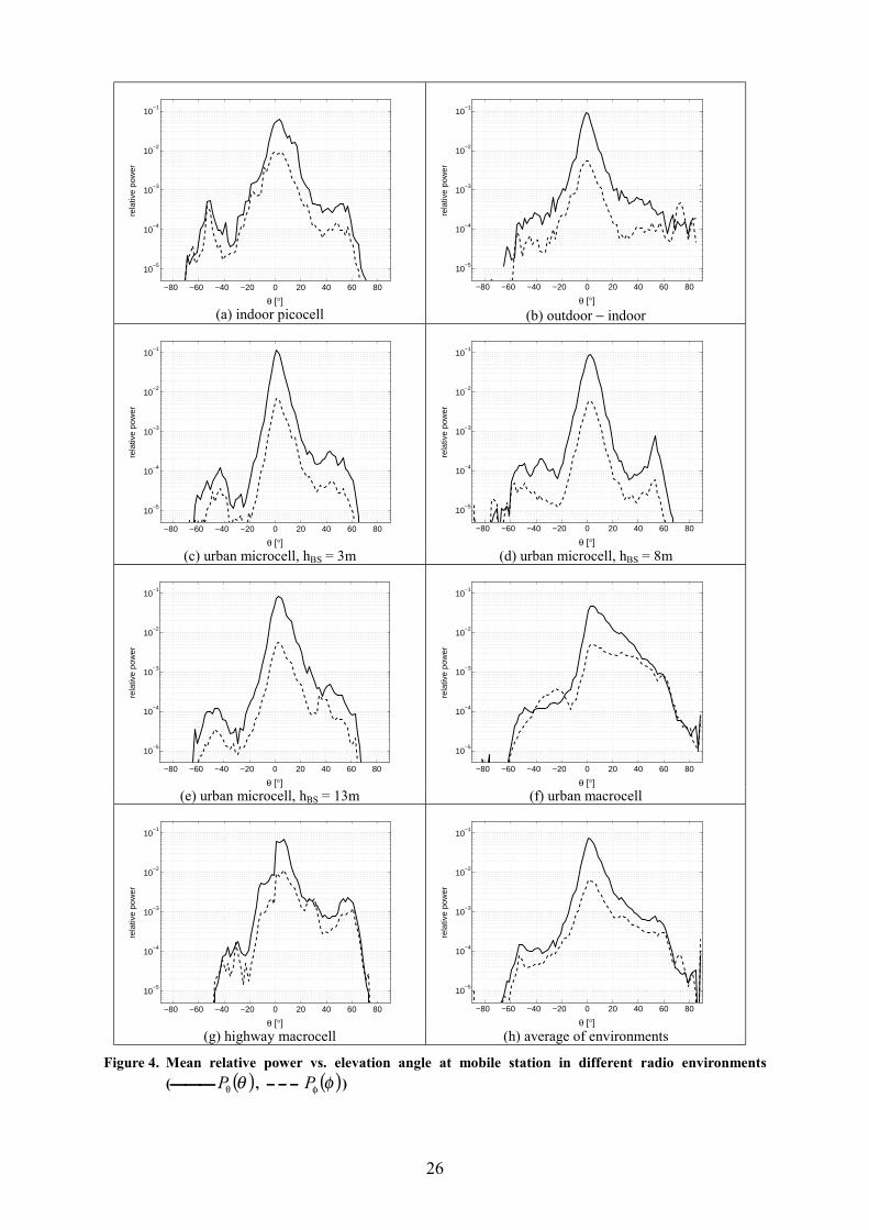
type as well as on the BS antenna height and BS−MS distance. Fig. 4 presents the mean relative power vs.

elevation angle in different environments. Also the average of all distributions is presented. The figure

demonstrates that the EPD depends on the environment and BS antenna height. In all environments dominated

by NLOS channels the shape of the EPD is similar for angles close to horizontal plane: the power decays roughly

exponentially on both sides of the peak of the EPD, until approximately 1 % of the peak power. Both the slope of

the exponential decay and the shape of the EPD outside the main lobe depend on the environment. It should be

noted, though, that in all environments most of the power is concentrated in small positive elevation angles. This

is in agreement with measurements by Lee and Brandt [20], who showed that most of the power is concentrated

in elevation angles lower than 16° above horizontal level.

In the indoor picocell measurements significant portion of the mobile routes contains LOS, which can be seen in

the θ-polarized EPD in Fig. 4(a) as peaks in the angle range of 10° to 20° above horizontal plane. The LOS

components with high elevation angles make the main lobe of the distribution wider also in the highway

macrocell measurements. In the urban outdoor case the EPD becomes asymmetrical and more power is received

at high elevation angles when the BS antenna is raised above the rooftop level. The negative slope of the EPD

changes hardly at all. For large antenna heights also the XPR decreases for increasing elevation angle. In the

urban macrocell case the XPR is approximately 0 dB for elevation angles above 60°. In the indoor picocell and

outdoor−indoor cases the received power outside the main lobe is notably higher than in the outdoor

measurements, most likely due to reflections from the ceiling. Similarly, the effect of the car can be seen as

distortions in the EPD of the highway macrocell.

The elevation power distribution is described by the median elevation angle ( θM ), mean elevation angle (θ ),

rms elevation spread ( θσ ), defined as:

10

( )21cos that so ,

2/

=∫−

θ

πθ θθθ

M

dpM (6)

( ) θθθθθπ

π

dp∫−

=2/

2/

cos (7)

[ ] ( ) θθθθθσπ

πθ dp cos

2/

2/

2

∫−

−= (8)

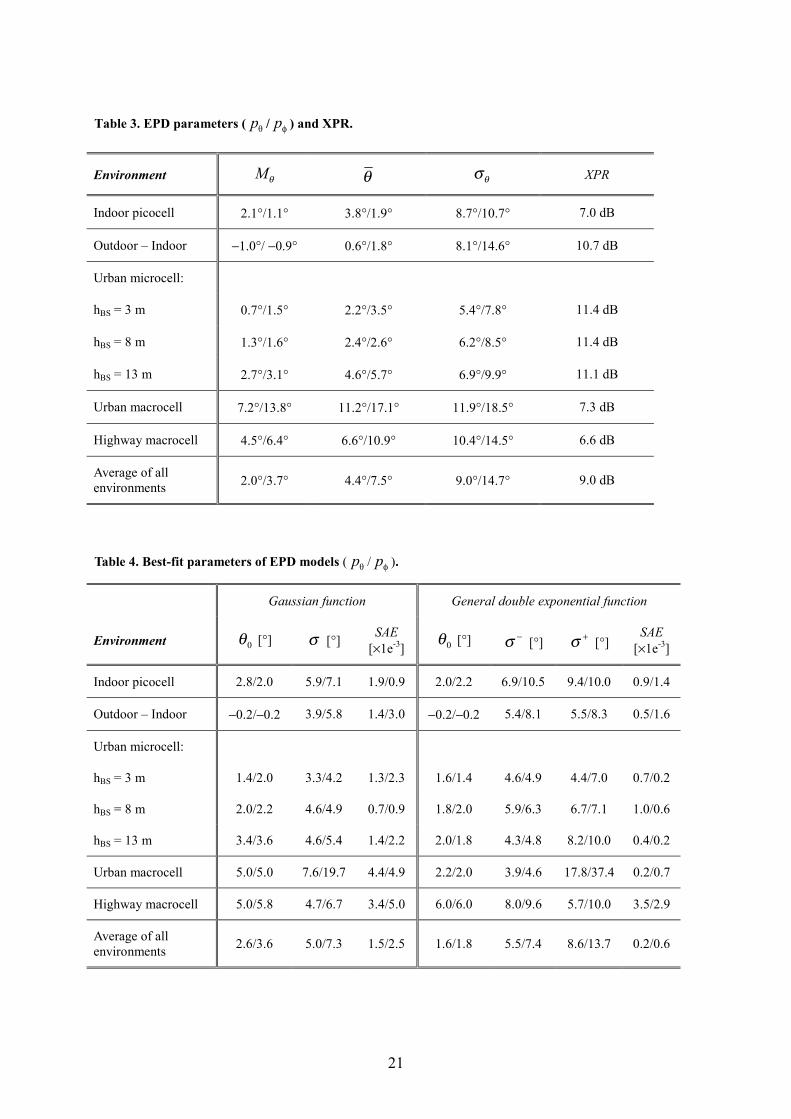
where p(θ) is either pθ(θ) or pφ(θ). The parameters of the measured EPDs of all environments are presented in

Table 3, from which the following observations can be made:

1) The rms elevation angle spread is larger for horizontal polarization in all environments.

2) In all outdoor environments the mean elevation angle is higher for horizontal polarization. In indoor picocell

the situation is the opposite, due to the large portion of LOS measurements.

3) In all environments the mean elevation angle is higher than the median, i.e. the distribution is asymmetrical

so that the spread is larger for high elevation angles than for low angles.

4) In urban environment the mean and median elevation angle, as well as the elevation spread, increase when

the BS antenna height increases. A clear step in mean values can be seen between BS antenna heights 8 and

13 m in the urban microcell case.

C. Model for Elevation Power Distribution

It is proposed in [9] that the EPD has Gaussian shape in urban environment, when no LOS exists between MS

and BS. However, as was observed in the previous section, the distribution is often not symmetrical about its

peak value, but it decreases more rapidly on the negative side. Particularly this seems to be the case for BS

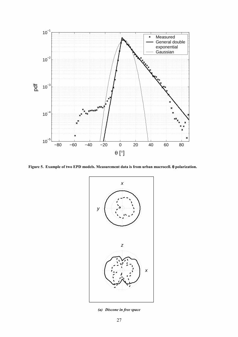
antenna heights larger than 10 m, which is common for outdoor base stations also in urban environments. Fig. 5

presents the measured EPD for θ-polarization in urban macrocell environment together with two best-fit

distribution functions:

11

1) Gaussian function:

( ) ( )

−∈

−−=2

,2

,2

exp 2

20

1ππθ

σθθθ Ap (9)

2) General double exponential function3:

( )

∈

−−

−∈

−−

=

+

−

2, ,

2exp

,2

,2

exp

00

2

00

2

πθθσ

θθ

θπθσ

θθ

θ

A

A

p (10)

In Eqs. (9,10) ( )θp is either ( )θθp or ( )θφp , 0θ is the peak elevation angle, and parameters σ, σ−, and σ+

control the spread of the functions. Coefficients 1A and

2A are set so that (1) is satisfied.

As can be seen in Fig. 5, in the case of an asymmetrical EPD the fitted symmetrical Gaussian function

( °= 0.50θ , °= 6.7σ ) does not give an accurate description of the EPD. Instead, the fitted general double

exponential function ( °= 2.20θ , °=− 9.3σ , °=+ 8.17σ ) gives an accurate match with measured data for values

larger than 0.7 % of the peak value. In order to find a representative statistical model for the elevation power

distribution, and to study the effect of the model on the obtained mean effective gain of a mobile antenna, we

fitted the measured power distributions in each environment to both model functions, by minimizing the squared

approximation error (SAE) of the fitted curves, defined as:

( ) ( )[ ] θθθπ

π

dppSAE measfit∫−

−=2/

2/

2 (11)

where pfit and pmeas are the modeled and measured distributions, respectively. Table 4 presents the best-fit

parameters and approximation error of both functions. It can be seen that for most environments the SAE of the

double exponential function is smaller than that of the Gaussian function, which indicates that the former yields

better match with the experimental data. The difference is clearest for the cases with largest BS antenna heights

(urban macrocell, urban microcell with hBS=13 m).

3If the spread parameters σ− and σ+ are equal the double exponential function is called Laplacian function

12

In [9], Taga reported considerably larger values for the mean elevation angle and standard deviation of the

Gaussian distribution derived from urban macrocell measurements in central Tokyo. However, the urban

environment in Tokyo is quite different from that of Helsinki, which could explain the difference. Also the BS

antenna height in his measurements was significantly larger (87 m) than in our measurements (27 m and 21 m),

increasing the portion of power propagated over building rooftops.

D. Cross Polarization Power Ratio

In the case of vertically polarized transmission, the XPR is defined as the power ratio of θ- and φ-polarized

components of the mean incident field. The XPR was obtained from the measurement data as the ratio of the

integrals of the mean relative incident power vs. elevation angle (see Table 1):

( )( ) θθ

θθ

dP

dPXPR

∫∫

φ

= θ(12)

The resulting XPR in each radio environment is shown in Table 3. The highest XPR values are obtained in the

urban microcell environment; the XPR is approximately 11 dB for all BS antenna heights. XPR is close to 11 dB

also in the outdoor-indoor case. Instead, for the indoor picocell, urban macrocell, and highway macrocell cases

the XPR is close to 7 dB. In the existing literature few measurements of the XPR at the mobile station have been

reported. In measurements presented in [21], the median “cross-polarization coupling”, which is equal to the

reciprocal of the XPR, was found to be as high as –2.5 dB inside and –3.5 dB outside houses in a residential area

at 800 MHz. The values are clearly lower than what we measured at 2.15 GHz. According to measurements by

Lee [22] and Taga [9], the XPR in urban macrocell environment is between 4 dB and 9 dB at 900 MHz. This is

comparable to our measurements at 2.15 GHz, although the BS antenna height and BS−MS distance are

considerably smaller. According to measurements by Lee and Yeh [22], the differences between the two cross

coupling coefficients (VP→HP, HP→VP) are less than 2 dB. This indicates that XPR at the mobile station is

comparable to the XPR at the base station. In [23] the mean XPR at the base station was found to be 7 dB in

urban macrocell at 463 MHz when a vertically polarized antenna was used at the mobile station.

In our urban microcell and outdoor-indoor measurements the range was considerably smaller than in the above

references. This would explain the higher obtained XPR values, under the assumption that the number of

depolarizing reflections and diffractions on the propagation path increases when the separation between the

13

transmitter and receiver increases. In [24], XPR at the base station was found to be close to 10 dB in urban

environment at 1800 MHz, and building penetration had minor influence on the XPR. In the highway macrocell

measurements the close scattering from the bodywork of the car most probably decreases the XPR. Also in the

indoor picocell measurements the low XPR value can be explained by the high number of close-proximity

scatterers around the mobile.

V. MEG COMPARISON OF HANDSET ANTENNAS

A. Evaluated Antenna Configurations

To evaluate MEG as a parameter describing the handset antenna performance we picked three typical handset

antennas: a commercial GSM1800 handset with an external meandered monopole antenna, and simulated

meandered monopole (MEMO) and planar inverted patch (PIFA) antennas attached to a handset model. In

addition, we took an omnidirectional discone antenna for reference. We measured the 3-D gain patterns of the

discone antenna and the GSM1800 handset in an anechoic chamber with a grid of 10° in both elevation and

azimuth. The measurement frequency was 2154 MHz for the discone and 1747 MHz for the GSM1800 handset.

Although the power distributions were obtained from measurements at 2154 MHz carrier frequency, they can be

assumed valid also at 1800 MHz frequency range; the frequency difference is so small that the same propagation

mechanisms are effective for waves at both frequencies. The discone was measured in free space only, while the

GSM1800 handset was measured both in free space and beside a model of human head and shoulders. In free

space the handset was oriented vertically, but when placed beside the model it was tilted 60° degrees from

vertical to correspond to a natural usage position. The handset touched the ear of the model. The used model was

Torso Phantom V2.0 by Schmidt & Partner Engineering AG, and it was filled with brain-simulating liquid.

We simulated the 3-D gain patterns of the MEMO and PIFA by using a commercial FDTD program (XFDTD,

version 5.1 Bio-Pro by Remcom, Inc.). Both antennas were attached to the top of a metallic chassis acting as the

body of a mobile phone. The simulations were performed both in free space and beside a head model. The

simulation frequency was 2154 MHz. In free space the phone chassis were oriented vertically. Beside the head,

they were oriented according to the intended use position specified by CENELEC [25]. The phone was tilted 74°

from vertical and 10° from the ear towards the cheek, as described in [26]. A distance of 5 mm was left between

the head and phone chassis, corresponding to the actual position of the metallic chassis of a mobile phone. The

14

used head model was an FDTD mesh with 2.5 mm voxel resolution remeshed from a standard human head and

shoulders model obtained from the software provider.

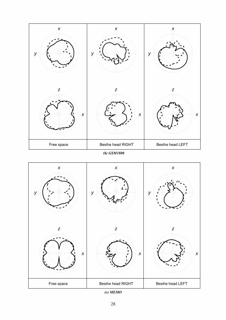
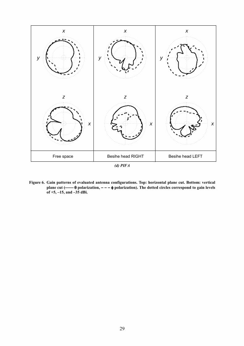
In both the measurements and simulations the head model was in upright position, and the nose pointed towards

positive y-axis (see Fig. 1). The patterns were measured and simulated for the handset placed on both right and

left side of the head, i.e. on the positive and negative x-axis sides, respectively. The horizontal (xy-plane) and

vertical (xz-plane) cuts of the power gain patterns of all antenna configurations are presented in Fig. 6.

B. Mean Effective Gains of Antennas

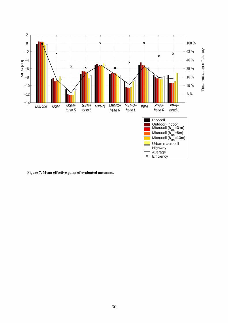
We computed the MEGs of all evaluated antenna configurations using [9, Eq. (6)]. The distribution of the

incident power was assumed uniform in azimuth. As the power distribution in elevation and cross polarization

power ratio we used the data obtained from the experiments and presented in Section IV. Fig. 7 shows the MEG

of each antenna configuration in all radio environments, together with the average MEG and the total antenna

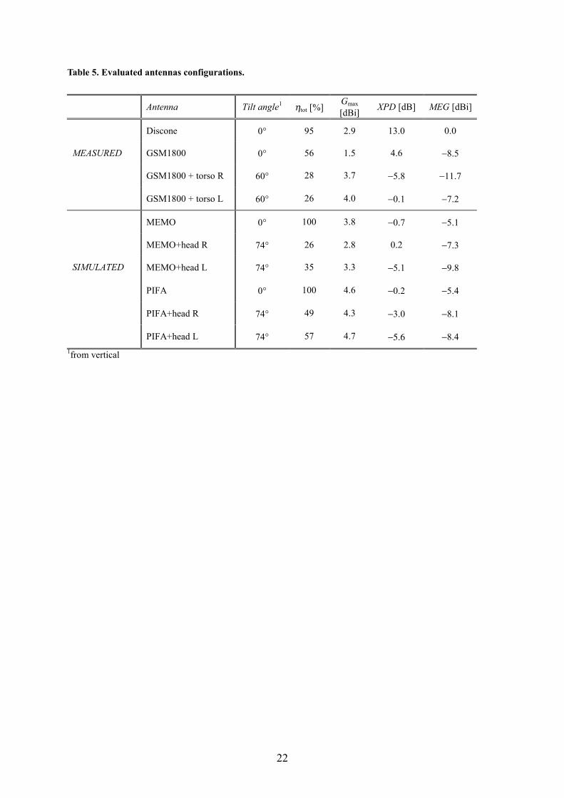
efficiency. Table 5 presents the average MEG, maximum gain, total antenna efficiency, and the cross-

polarization discrimination (XPD) of each configuration. The cross-polarization discrimination is given by:

( )

( ) φθθφθ

φθθφθ

π π

πφ

π π

πθ

ddG

ddGXPD

cos,

cos,

2

0

2/

2/

2

0

2/

2/

∫ ∫

∫ ∫

−

−= (13)

The total antenna efficiency (including the dielectric losses due to the head model) is obtained by:

( ) ( )[ ] φθθφθφθπ

ηπ π

πφθ ddGG cos,,

41 2

0

2/

2/tot ∫ ∫

−

+= (14)

The reference level in the gain measurement of the GSM1800 handset was the nominal maximum transmission

power. Note that the MEG of an antenna in an artificial isotropic environment − i.e. for

( ) ( )π

φθφθ41,,θ == φpp , 1=XPR − is equal to the total antenna efficiency divided by two. Based on Table 5,

no direct connection can be found between the MEG of an antenna configuration and its total efficiency or gain.

Furthermore, it turned out that in most cases the differences in the MEG values could not be predicted directly

15

by analyzing the plane cuts of the radiation pattern. Only clearly negative XPD with dominating φ polarization

predicted low MEG values.

Fig. 7 shows that the differences in MEG are clearly larger between antennas than between radio environments.

This is understandable, since in all environments most of the power is received at small positive elevation angles

(see Fig. 4). In effect, the XPR seems to explain most of the environmental dependence of the MEG, as will be

presented below. The reference discone has by far the highest MEG: close to 0 dBi in all environments. This is

due to its omnidirectional radiation pattern, high efficiency, and high cross-polarization discrimination. It should

be noted that also the MEMO and PIFA have high efficiency in free space, but still their MEGs are significantly

lower: of the order of −5 dBi.

When placed beside the head model, the total efficiency of the MEMO drops by 5.9/4.6 dB, depending on the

side of the head (R/L). At the same time, the average MEG drops by 2.2/4.7 dB. Fig. 6 (c) shows that the θ-

polarized pattern of the MEMO in free space has a minimum in the horizontal plane. Instead, beside the head the

maximum of the θ-polarized pattern is produced at the horizontal plane. On the right side of the head θ

polarization dominates, which partly compensates for the decreased efficiency. For MEMO, the difference in

MEGs on the two sides of the head is 2.5 dB. For PIFA, the total antenna efficiency drops by 3.1/2.4 dB when

placed beside the head, and the MEG drops on average by 2.7/3.0 dB.

The average MEG of the measured GSM1800 handset increases by 1.3 dB when the handset is placed on the left

side of the head of the human body model, although the total efficiency drops by 3.3 dB from the free space

value. On the right side of the head the average MEG is 4.5 dB lower than on the left side, although the total

efficiency is 0.3 dB higher. The maximum gain of the antenna configuration is almost the same on both sides of

the head (note that in free space the gain is lower). The result clearly indicates that maximum gain or total

efficiency of an antenna is not enough to describe its performance in practical environments.

When any of the two simulated antennas is placed on the left side of the head, the highest MEG values are

obtained in environments with lowest XPR (see Fig. 7). The behavior is partly explained by the XPD values of

the antenna configurations, which are lower on the left side than the right (see Table 5). The opposite happens

for the measured GSM1800, which had the antenna located on the opposite corner of the handset. The highest

variation of MEG values between different environments is obtained for antenna configurations with negative

XPDs.

16

It has been observed also previously [27] that the MEG of a handset antenna depends on which side of the head

the user holds the handset. In [27], the average user influence at 1800 MHz frequency was found to be a loss of

10 dB for a helical antenna, and 3 dB for a patch antenna. In our analysis the average decrease in MEG due to

the user was 0.8 dB, 3.3 dB and 2.8 dB for the measured GSM1800 and the simulated MEMO and PIFA,

respectively. However, we only modeled the head of the user (also the shoulders for the measured handset), and

not the hand or full body, which partly explains the difference.

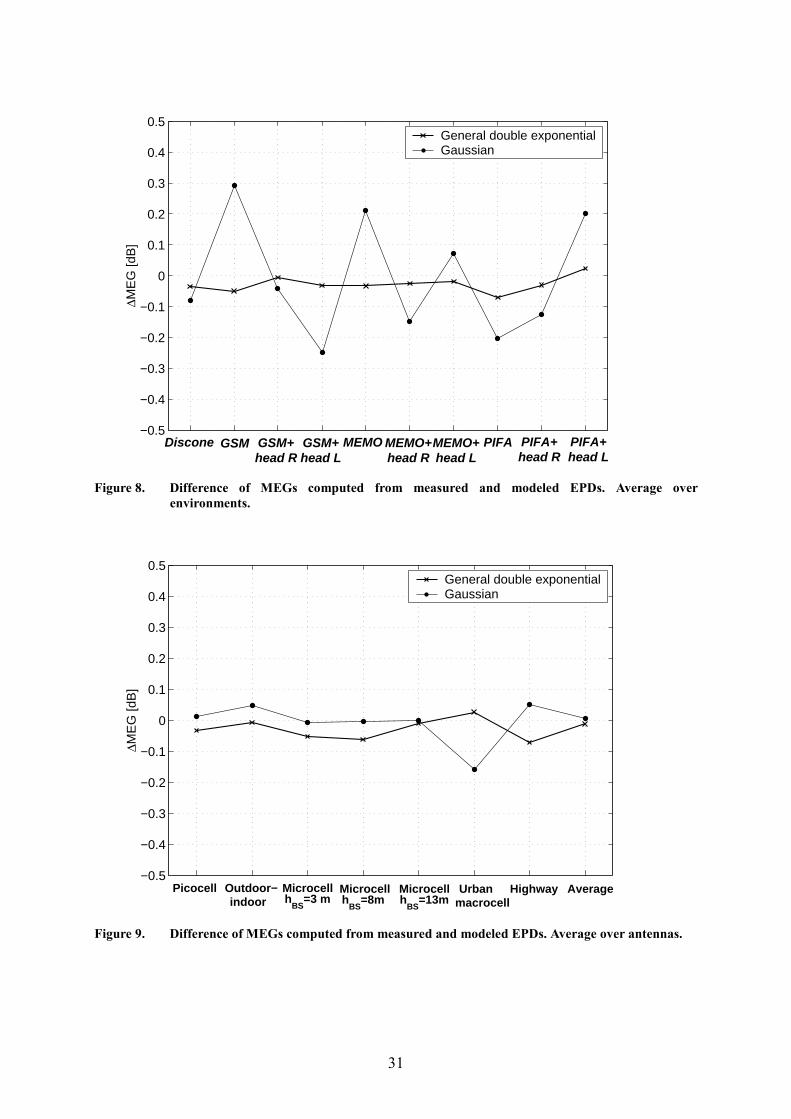
C. Effect of Model Distribution on MEG

In order to evaluate the two models for the elevation power distribution (see Sec. IV.C), we repeated the MEG

computation for the same antennas using the model distributions, fitted separately for each environment using

parameters given in Table 4. For XPR, the values obtained directly from measurements (presented in Table 3)

were used. The average differences between the MEGs obtained for the measured and the two modeled EPDs are

plotted in Figs. 8 and 9. The MEG errors of both models are small, less than 0.5 dB for the Gaussian distribution,

and less than 0.1 dB for the General double exponential distribution. The differences between antennas (Fig. 8)

are larger than the differences between the environments (Fig. 9). This can be understood based on the results

shown in the previous section, showing that the environment type has quite small effect on the obtained MEG.

VI. CONCLUSIONS

We applied a novel technique for measuring the angular distribution and cross-polarization ratio of the incident

power at the mobile station in different types of propagation environments. This information is needed in the

evaluation of mobile handset antenna performance in realistic operating environments. The results show that in

NLOS situations the power distribution in elevation has a shape of a double-sided exponential function, with

different slopes on the negative and positive sides of the peak. The slopes and the peak elevation angle depend

on the environment and base station antenna height. We noticed that the distribution becomes asymmetrical

when the antenna is raised above the rooftop level in urban environment. With lower BS antenna heights the

power is concentrated only slightly above the horizontal plane.

The measured cross-polarization power ratio was smallest in indoor picocell and urban macrocell environments,

of the order of 7 dB. A similar value was obtained also when the mobile antenna was placed inside a person car

17

in measurements on a highway. In urban microcell and outdoor-indoor measurements with relatively short

ranges the XPR was fairly large, approximately 11 dB.

We applied the experimental data for analysis of the mean effective gain of several practical handset antennas.

The MEG values varied from approximately −5 dBi in free space to less than −11 dBi beside the head model.

These values are considerably lower than the 0 dBi typically used in system specifications, e.g. [28]. The result

shows that considering only the maximum gain or total efficiency of the antenna is not enough to describe its

performance in practical operating conditions. In all measured environments the cross polarization coupling was

fairly small, indicating that the polarization of a handset antenna should be matched to that of the BS antenna, to

obtain best performance. However, the polarization of the antenna is sensitive to the usage position of the

handset, which should be considered in antenna design.

For most antennas the environment type has little effect on the MEG, but clear differences exist between

antennas. The MEG also depends on which side of the head the user holds the handset. Errors in MEG values

caused by using any of the two power distribution models instead of the measured power distributions were

small: on average less than 0.5 dB for the Gaussian distribution, and less than 0.1 dB for the General double

exponential distribution.

In this contribution we only considered the mean value of the effective gain of a handset antenna. However, it is

also important to know the probability levels of which a certain portion of the total incident power is received.

The measurements described in this paper allow the analysis of such instantaneous reception efficiency of a

handset, as well as more sophisticated analysis like estimation of polarization diversity gain, which are important

issues for further studies.

VII. ACKNOWLEDGEMENTS

The authors wish to thank Martti Toikka, Lasse Vuokko, Jani Ollikainen, Pasi Suvikunnas, and Eero Rinne for

their help in carrying out the radio channel measurements. The work was partially funded by the National

Technology Agency of Finland (TEKES), and the Graduate School in Electronics, Telecommunications and

Automation (GETA). Financial support from the Finnish Society of Electronics Engineers, HPY Foundation,

Nokia Foundation, and Wihuri Foundation is also gratefully acknowledged.

18

VIII. REFERENCES

[1] J. B. Andersen and F. Hansen, “Antennas for VHF/UHF Personal Radio: A Theoretical and ExperimentalStudy of Characteristics and Performance,” IEEE Transactions on Vehicular Technology, vol. 26, no. 4,pp. 349−357, November 1977.

[2] H. Arai, N. Igi, and H. Hanaoka, “Antenna-Gain Measurement of Handheld Terminals at 900 MHz,”IEEE Transactions on Vehicular Technology, vol. 46, no. 3, pp. 537-543, August 1997.

[3] I. Z. Kovács, P. C. F. Eggers, and K. Olesen, “Comparison of Mean Effective Gains of different DCS1800handset antennas in urban and suburban environments”, Proc. IEEE 48th Vehicular TechnologyConference (VTC98), Ottawa, Ontario, Canada, May 18-21, 1998, pp. 1974-1978.

[4] K. Sulonen, K. Kalliola, and P. Vainikainen, “Comparison of Evaluation Methods for Mobile HandsetAntennas,” Proceedings of Millennium Conference on Antennas & Propagation (AP2000), Davos,Switzerland, April 9-14, 2000, CD-ROM SP-444 (ISBN 92-9092-776-3), paper p0870.pdf.

[5] B. M. Green and M. A. Jensen, “Diversity Performance of Dual-Antenna Handsets Near OperatorTissue,” IEEE Transactions on Vehicular Technology, vol. 48, no. 7, pp. 1017-1024, July 2000.

[6] G. F. Pedersen and J. Bach Andersen, “Handset Antennas for Mobile Communications: Integration,Diversity, and Performance,” Chapter 5 in Review of Radio Science 1996-1999, editor W.R. Stone,Oxford, Oxford University Press, 1999, 970 p.

[7] H. Arai, Measurement of Mobile Antenna Systems, Boston, Artech House, 2001, 214 p.

[8] B. G. H. Olsson, “Simplistic Field Distribution Estimation of a Scattered Field Measurement Room,”Proc. IEEE 51st Vehicular Technology Conference (VTC2000-Spring), Tokyo, Japan, 15-18 May, 2000,vol. 3, pp. 2482-2486.

[9] T. Taga, “Analysis for mean effective gain of mobile antennas in land mobile radio environments,” IEEETransactions on Vehicular Technology, vol. 39, no. 2, pp. 117-131, May 1990.

[10] M. B. Knudsen, G. F. Pedersen, B. G. H. Olsson, K. Olesen, and S.-Å. A. Larsson, “Validation of HandsetAntenna Test Methods,” Proc. IEEE 52nd Vehicular Technology Conference (VTC2000-Fall), Boston,MA, USA, 24-28 September, 2000, vol. 4, pp. 1669-1676.

[11] A. Kuchar, J.-P. Rossi, and E. Bonek, “Directional Macro-Cell Channel Characterization from UrbanMeasurements,” IEEE Transactions on Antennas and Propagation, vol. 48, no. 2, pp. 137-146, February2000.

[12] H. Laitinen, K. Kalliola, and P. Vainikainen, “Angular Signal Distribution and Cross-Polarization PowerRatio Seen by a Mobile Receiver at 2.15 GHz,” Proceedings of Millennium Conference on Antennas &Propagation (AP2000), Davos, Switzerland, April 9-14, 2000, CD-ROM SP-444 (ISBN 92-9092-776-3),paper p1133.pdf.

[13] S. Qu and T. Yeap, “A three-dimensional scattering model for fading channels in land mobileenvironment,” IEEE Transactions on Vehicular Technology, vol. 48, no. 3, May 1999, pp. 765-781.

[14] K. Kalliola, H. Laitinen, L. I. Vaskelainen, and P. Vainikainen, “Real-time 3D Spatial-Temporal Dual-polarized Measurement of Wideband Radio Channel at Mobile Station,” IEEE Transactions onInstrumentation and Measurement, vol. 49, no. 2, pp. 439-448, April 2000.

[15] R. H. Clarke, “3-D Mobile Radio Channel Statistics,” IEEE Transactions on Vehicular Technology,vol. 46, no. 3, August 1997, pp. 798-799.

[16] R. H. Clarke, “A statistical theory of mobile radio reception,” Bell. Syst. Tech. J., vol. 47, July/Aug. 1968,pp. 957-1000.

19

[17] T. Aulin, “A Modified Model for the Fading Signal at a Mobile Radio Channel,” IEEE Transactions onVehicular Technology, vol. 28, no. 3, pp. 182-203, August 1979.

[18] J. Kivinen, T. Korhonen, P. Aikio, R. Gruber, P. Vainikainen, S.-G. Häggman, “Wideband Radio ChannelMeasurement System at 2 GHz”, IEEE Transactions on Instrumentation and Measurement, vol. 48, no. 1,February 1999, pp. 39-44.

[19] J. Laurila, K. Kalliola, M. Toeltsch, K. Hugl, P. Vainikainen, and E. Bonek, “Wideband 3-DCharacterization of Mobile Radio Channels in Urban Environment”, To be Published in IEEETransactions on Antennas and Propagation, 2001.

[20] W. C.-Y. Lee and R. H. Brandt, “The Elevation angle of Mobile Radio Signal Arrival,” IEEETransactions on Communications, vol. COM-21, no. 11, November 1973, pp. 1194−1197.

[21] D. C. Cox, R. R. Murray, H. W. Arnold, A. W. Norris, and M. F. Wazowicz, “Cross-PolarizationCoupling Measured for 800 MHz Radio Transmission In and Around Houses and Large Buildings,” IEEETransactions on Antennas and Propagation, vol. 34, no. 1, January 1986, pp. 83−87.

[22] W. C.-Y. Lee and Y.S. Yeh, “Polarization Diversity System for Mobile Radio,” IEEE Transactions onCommunications, vol. COM-20, no. 5, October 1972, pp. 912−923.

[23] R. Vaughan, “Polarization Diversity in Mobile Communications,” IEEE Transactions on VehicularTechnology, vol. 39, no. 3, August 1990, pp. 177−186.

[24] P. C. F. Eggers, I. Z.Kovács, and K. Olesen, “Penetration effects on XPD with GSM1800 handsetantennas, relevant for BS polarization diversity for indoor coverage,” Proc. IEEE 48th VehicularTechnology Conference (VTC98), Ottawa, Ontario, Canada, May 18-21, 1998, pp. 1959-1963.

[25] European specification (ES 59005), Considerations for the Evaluation of Human Exposure toElectromagnetic Fields (EMFs) from Mobile Telecommunication Equipment (MTE) in the FrequencyRange 30 MHz - 6 GHz, Brussels, Belgium, CENELEC, October 1998, 81 p.

[26] J. T. Rowley and R. B. Waterhouse, “Performance of Shorted Microstrip Patch Antennas for MobileCommunications Handsets at 1800 MHz,” IEEE Transactions on Antennas and Propagation, vol. 47, no.5, May 1999, pp. 815-822.

[27] G. F. Pedersen, J. Ø. Nielsen, K. Olesen, and I. Z. Kovács, “Measured Variation in Performance ofHandheld Antennas for a Large Number of Test Persons,” Proc. IEEE 48th Vehicular TechnologyConference (VTC98), Ottawa, Ontario, Canada, May 18-21, 1998, pp. 505-509.

[28] ETSI Technical Report TR 101 112 V3.2.0 (1998-04), Universal Mobile Telecommunications System(UMTS); Selection procedures for the choice of radio transmission technologies of the UMTS (UMTS30.03 version 3.2.0), European Telecommunications Standards Institute, 1998, 84 p.

20

TABLES

Table 1. Definitions of angular power distributions. Subscripts denote polarizations.

Definition Azimuth Elevation

Instantaneous power asa function of incidenceangle.

( ) ( )

( ) ( )∫ ∫

∫ ∫

φφ

θθ

=

=

τ θ

τ θ

τθθτφθφ

τθθτφθφ

ddhP

ddhP

ii

ii

cos,,

cos,,

2,,

2,, ( ) ( )

( ) ( )∫ ∫

∫ ∫

φ,φ

θ,θ

=

=

τ φ

τ φ

τφτφθθ

τφτφθθ

ddhP

ddhP

ii

ii

2,

2,

,,

,,

Mean relative power asa function of incidenceangle.

( ) ( )( ) ( )[ ]

( ) ( )( ) ( )[ ]∑

∫

∑∫

= φ

φφ

= φ

+=

+=

N

i ii

i

N

i ii

i

dPPP

NP

dPPP

NP

1 ,,θ

,

1 ,,θ

,θθ

1

1

φφφφ

φ

φφφφ

φ ( ) ( )( ) ( )[ ]

( ) ( )( ) ( )[ ]∑

∫

∑∫

= φθ

φφ

= φθ

θθ

+=

+=

N

i ii

i

N

i ii

i

dPPP

NP

dPPP

NP

1 ,,

,

1 ,,

,

cos1

cos1

θθθθθ

θ

θθθθθ

θ

Power distributions inazimuth (APD) andelevation (EPD).

( ) ( )( )

( ) ( )( )∫

∫

φ

φφ =

=

φφφ

φ

φφφφ

dPP

p

dPPpθ

θθ ( ) ( )

( )

( ) ( )( )∫

∫

φ

φφ

θ

θθ

=

=

θθθ

θθ

θθθθθ

dPP

p

dPPp

cos

cos

Table 2. Amount of collected data.

Environment Route length Snapshots LOS NLOS

Indoor picocell (Airport) 260 m N = 9 800 40 % 60 %

Outdoor – Indoor (Office) 220 m N = 8 300 0 % 100 %

Urban microcell

(hBS =3/8/13 m)

3×1200 m

= 3600 m

3×51 000

N=153 00022 % 78 %

Urban macrocell

(hBS = 21/27 m)2560 m N=100 600 4 % 96 %

Highway macrocell 2500 m N = 47 600 25+45* % 30 %

TOTAL 9140 m N=319 300 23 % 77 %*LOS obstructed by trees

21

Table 3. EPD parameters ( θp / φp ) and XPR.

Environment θM θ θσ XPR

Indoor picocell 2.1°/1.1° 3.8°/1.9° 8.7°/10.7° 7.0 dB

Outdoor – Indoor −1.0°/ −0.9° 0.6°/1.8° 8.1°/14.6° 10.7 dB

Urban microcell:

hBS = 3 m 0.7°/1.5° 2.2°/3.5° 5.4°/7.8° 11.4 dB

hBS = 8 m 1.3°/1.6° 2.4°/2.6° 6.2°/8.5° 11.4 dB

hBS = 13 m 2.7°/3.1° 4.6°/5.7° 6.9°/9.9° 11.1 dB

Urban macrocell 7.2°/13.8° 11.2°/17.1° 11.9°/18.5° 7.3 dB

Highway macrocell 4.5°/6.4° 6.6°/10.9° 10.4°/14.5° 6.6 dB

Average of allenvironments 2.0°/3.7° 4.4°/7.5° 9.0°/14.7° 9.0 dB

Table 4. Best-fit parameters of EPD models ( θp / φp ).

Gaussian function General double exponential function

Environment 0θ [°] σ [°] SAE[×1e-3] 0θ [°] −σ [°] +σ [°]

SAE[×1e-3]

Indoor picocell 2.8/2.0 5.9/7.1 1.9/0.9 2.0/2.2 6.9/10.5 9.4/10.0 0.9/1.4

Outdoor – Indoor −0.2/−0.2 3.9/5.8 1.4/3.0 −0.2/−0.2 5.4/8.1 5.5/8.3 0.5/1.6

Urban microcell:

hBS = 3 m 1.4/2.0 3.3/4.2 1.3/2.3 1.6/1.4 4.6/4.9 4.4/7.0 0.7/0.2

hBS = 8 m 2.0/2.2 4.6/4.9 0.7/0.9 1.8/2.0 5.9/6.3 6.7/7.1 1.0/0.6

hBS = 13 m 3.4/3.6 4.6/5.4 1.4/2.2 2.0/1.8 4.3/4.8 8.2/10.0 0.4/0.2

Urban macrocell 5.0/5.0 7.6/19.7 4.4/4.9 2.2/2.0 3.9/4.6 17.8/37.4 0.2/0.7

Highway macrocell 5.0/5.8 4.7/6.7 3.4/5.0 6.0/6.0 8.0/9.6 5.7/10.0 3.5/2.9

Average of allenvironments 2.6/3.6 5.0/7.3 1.5/2.5 1.6/1.8 5.5/7.4 8.6/13.7 0.2/0.6

22

Table 5. Evaluated antennas configurations.

Antenna Tilt angle1 ηtot [%] Gmax

[dBi] XPD [dB] MEG [dBi]

Discone 0° 95 2.9 13.0 0.0

MEASURED GSM1800 0° 56 1.5 4.6 −8.5

GSM1800 + torso R 60° 28 3.7 −5.8 −11.7

GSM1800 + torso L 60° 26 4.0 −0.1 −7.2

MEMO 0° 100 3.8 −0.7 −5.1

MEMO+head R 74° 26 2.8 0.2 −7.3

SIMULATED MEMO+head L 74° 35 3.3 −5.1 −9.8

PIFA 0° 100 4.6 −0.2 −5.4

PIFA+head R 74° 49 4.3 −3.0 −8.1

PIFA+head L 74° 57 4.7 −5.6 −8.41from vertical

23

FIGURES

Figure 1. Spherical coordinate system.

z

x

y

θ = −90°

Antenna

E

θ = 0°φ = 90°

E

θ

φ

θ

φ

θ = 90°

θ = 0°φ = −90°

θ = 0°φ = 0°

Incident wave

antennamovingdirection

24

Figure 2. Measurement routes in the center of Helsinki.

10-20 m21-25 m26-30 m

>30 m

Building height

S

W E

NMS Route macrocellBS Macrocell

MS Route microcellBS Microcell

100 2000 300 400 500 m

25

30

−150

60

−120

90 −90

120

−60

150

−30

180

0

.0025.005

.01.02

.04.08

(a)

30

−150

60

−120

90 −90

120

−60

150

−30

180

0

.0025.005

.01.02

(b)Figure 3. Mean azimuth power distributions. (a) Urban microcell, hBS = 3 m. (b) Urban macrocell. Mobile

moving direction is 0°°°° ( ( )φθp , − − −− − −− − −− − − ( )φφp ).

26

−80 −60 −40 −20 0 20 40 60 80

10−5

10−4

10−3

10−2

10−1

θ [°]

rela

tive

pow

er

−80 −60 −40 −20 0 20 40 60 80

10−5

10−4

10−3

10−2

10−1

θ [°]

rela

tive

pow

er

(a) indoor picocell (b) outdoor − indoor

−80 −60 −40 −20 0 20 40 60 80

10−5

10−4

10−3

10−2

10−1

θ [°]

rela

tive

pow

er

−80 −60 −40 −20 0 20 40 60 80

10−5

10−4

10−3

10−2

10−1

θ [°]

rela

tive

pow

er

(c) urban microcell, hBS = 3m (d) urban microcell, hBS = 8m

−80 −60 −40 −20 0 20 40 60 80

10−5

10−4

10−3

10−2

10−1

θ [°]

rela

tive

pow

er

−80 −60 −40 −20 0 20 40 60 80

10−5

10−4

10−3

10−2

10−1

θ [°]

rela

tive

pow

er

(e) urban microcell, hBS = 13m (f) urban macrocell

−80 −60 −40 −20 0 20 40 60 80

10−5

10−4

10−3

10−2

10−1

θ [°]

rela

tive

pow

er

−80 −60 −40 −20 0 20 40 60 80

10−5

10−4

10−3

10−2

10−1

θ [°]

rela

tive

pow

er

(g) highway macrocell (h) average of environments

Figure 4. Mean relative power vs. elevation angle at mobile station in different radio environments( ( )θθP , −−−− −−−− −−−− ( )φφP )

27

−80 −60 −40 −20 0 20 40 60 8010

−5

10−4

10−3

10−2

10−1

θ [°]

pdf

Measured General doubleexponential Gaussian

Figure 5. Example of two EPD models. Measurement data is from urban macrocell. θθθθ polarization.

x

y

z

x

(a) Discone in free space

28

x

y

z

x

x

y

z

x

x

y

z

x

(b) GSM1800

x

y

z

x

x

y

z

x

x

y

z

x

(c) MEMO

Free space Besihe head RIGHT Besihe head LEFT

Free space Besihe head RIGHT Besihe head LEFT

29

x

y

z

x

x

y

z

x

x

y

z

x

(d) PIFA

Figure 6. Gain patterns of evaluated antenna configurations. Top: horizontal plane cut. Bottom: verticalplane cut ( θθθθ polarization, −−−− −−−− −−−− φφφφ polarization). The dotted circles correspond to gain levelsof +5, –15, and –35 dBi.

Free space Besihe head RIGHT Besihe head LEFT

30

Figure 7. Mean effective gains of evaluated antennas.

−14

−12

−10

−8

−6

−4

−2

0

2

ME

G [

dB

]

100 %

63 %

40 %

25 %

16 %

10 %

To

tal ra

dia

tio

n e

ffic

ien

cy

Discone GSM GSM+torso R

MEMO MEMO+head R

MEMO+head L

PIFA PIFA+head R

PIFA+head L

GSM+torso L

6 %

Picocell Outdoor−indoor Microcell (h

BS=3 m)

Microcell (hBS

=8m) Microcell (h

BS=13m)

Urban macrocell Highway Average Efficiency

31

−0.5

−0.4

−0.3

−0.2

−0.1

0

0.1

0.2

0.3

0.4

0.5∆M

EG

[dB

]General double exponentialGaussian

Discone GSM GSM+head L

MEMO MEMO+head R

MEMO+head L

PIFA PIFA+head R

PIFA+head L

GSM+head R

Figure 8. Difference of MEGs computed from measured and modeled EPDs. Average overenvironments.

−0.5

−0.4

−0.3

−0.2

−0.1

0

0.1

0.2

0.3

0.4

0.5

∆ME

G [d

B]

General double exponentialGaussian

Picocell Outdoor−indoor

Microcellh

BS=3 m

Microcellh

BS=8m

Microcellh

BS=13m

Urban macrocell

Highway Average

Figure 9. Difference of MEGs computed from measured and modeled EPDs. Average over antennas.