Animal Biodiversity and Conservation 27.1 (2004) A …abc.museucienciesjournals.cat/files/ABC-27-1-pp-515-529.pdf · Palabras clave: Datos de censo, Análisis integrado, Filtro de

515Animal Biodiversity and Conservation 27.1 (2004)

© 2004 Museu de Ciències NaturalsISSN: 1578–665X

Brooks, S. P., King, R. & Morgan, B. J. T., 2004. A Bayesian approach to combining animal abundance anddemographic data. Animal Biodiversity and Conservation, 27.1: 515–529.

AbstractA Bayesian approach to combining animal abundance and demographic data.— In studies of wild animals,one frequently encounters both count and mark–recapture–recovery data. Here, we consider an integratedBayesian analysis of ring–recovery and count data using a state–space model. We then impose a Leslie–matrix–based model on the true population counts describing the natural birth–death and age transitionprocesses. We focus upon the analysis of both count and recovery data collected on British lapwings(Vanellus vanellus) combined with records of the number of frost days each winter. We demonstrate how thecombined analysis of these data provides a more robust inferential framework and discuss how theBayesian approach using MCMC allows us to remove the potentially restrictive normality assumptionscommonly assumed for analyses of this sort. It is shown how WinBUGS may be used to perform theBayesian analysis. WinBUGS code is provided and its performance is critically discussed.

Key words: Census data, Integrated analysis, Kalman filter, Logistic regression, Ring–recovery data, State–space model, WinBUGS.

ResumenAproximación bayesiana para combinar abundancia y datos demográficos.— En estudios de animalessalvajes, es frecuente encontrarse tanto con datos de recuento como datos de marcaje–recaptura–recuperación. En el presente estudio consideramos un análisis integrado bayesiano de recuperación deanillas y datos de recuento utilizando un modelo de estado–espacio. Seguidamente aplicamos un modelobasado en las matrices de Leslie en los recuentos de población verdadera para describir los procesosnaturales de nacimiento–muerte y de transición de edades. Nos centramos en el análisis de los datos derecuento y de recuperación recopilados en avefrías europeas (Vanellus vanellus) en combinación con losregistros del número de días de helada de cada invierno. Demostramos cómo el análisis combinado deestos datos proporciona un marco inferencial más sólido, y discutimos cómo el enfoque bayesiano usandoMCMC nos permite eliminar los supuestos de normalidad potencialmente restrictivos que suelen adoptarseen análisis de este tipo. Se demuestra cómo puede utilizarse WinBUGS para realizar el análisis bayesiano.Se facilita el código WinBUGS, y se discute su funcionamiento.

Palabras clave: Datos de censo, Análisis integrado, Filtro de Kalman, Regresión logística, Datos derecuperación de anillas, Modelo de estado–espacio, WinBUGS.

S. P. Brooks, The Statistical Laboratory–CMS, Univ. of Cambridge, Wilberforce Road, Cambridge CB3 0WB,U.K.– R. King, CREEM, Univ. of St. Andrews, Buchanan Gardens, St. Andrews KY16 9LZ, U.K.– B. J. T.Morgan, Inst. of Matemathics, Statistics and Actuarial Science, Univ. of Kent, Canterbury CT2 7NF, U.K.

A Bayesian approach to combininganimal abundance and demographicdata

S. P. Brooks, R. King & B. J. T. Morgan

516 Brooks et al.

in the case of lapwings, the index data do notprovide a formal census of a national population,but may be regarded as estimating the populationsize for the set of sites at which observations takeplace. We also introduce the number of days eachyear that a Central England temperature fell belowzero, as a covariate to help describe the variation insurvival over time. We begin with a description ofthe population index data and associated model.

Population index data

The population index data are derived from theCommon Birds Census (CBC) which has beenthe main source of information on populationlevels for common British birds since it was es-tablished in 1962. More recently it has beenreplaced by the Breeding Bird Survey. Annualcounts are made at a number of sites around theUK and from these an index value is calculatedbased upon a statistical analysis of the datacollected (Ter Braak et al., 1994). The raw dataare not used, but the index provides a measure ofthe population level, taking account of the factthat each year only a small proportion of sites areactually surveyed. We shall consider the analysisof single–site data in Section 4. Here, we analysethe index values collected for adult females from1965 to 1998 inclusive and we omit data fromearlier years of the study during which the indexprotocol was being standardised. The data areplotted in (Besbeas et al., 2002). We denote theindex value for year t by yt and, for consistencywith the ring–recovery data described later, weassociate the year 1963 with the value t = 1, sothat we actually observe the values y3,...,y36.

Since these yt are only estimates, we first try toestimate the true underlying population levels thatwe will subsequently use as input into our systemmodel. Here we shall assume that

yt - N ( Na,t, y2) (1)

where Na,t represents the true underlying numbersof adult females aged $$$$$ 2 years at time t. Here y

2

is taken as a constant variance, although otherassumptions could also be made. For an index, aconstant variance seems reasonable; we do nothave access to the estimated standard errors re-sulting from the separate statistical analysis thathas resulted in the population index. Note that weestimate y

2 from the index data, and not from theraw survey data. This then describes the observa-tion process by which the estimates yt are derivedfrom the true underlying process Na,t.

We next need to describe the underlying systemprocess which provides a model for the evolution ofthe true underlying population size over time. Wefollow the notation of Besbeas et al. (2002), ratherthan Durbin & Koopman (1997). A natural modelwould be to assume that

Na,t - Bin (N1, t–1 + Na,t–1, a,t–1)

Introduction

Studies of wildlife populations often result in differentforms of data being collected from different sources.Useful data comprise capture–recapture data (of liveanimals), ring–recovery data (of dead animals), ra-dio–tagging (where the state of each animal is knownat all times), data on productivity (as in nest–recorddata, for example), location data and/or count data(estimates of total population size). By combiningdata from different sources, we obtain more robust(and self–consistent) parameter estimates that fullyreflect the information available. Previous studies ofcombined data of this sort include the analysis ofjoint capture–recapture and ring–recovery data(Catchpole et al., 1998; King & Brooks, 2002b),multi–site data (King & Brooks, 2002a; King & Brooks,2003) and joint ring–recovery and either census dataor population indices (Besbeas et al., 2002).

In this paper, we shall consider a Bayesian analy-sis of joint ring–recovery and population index data,revisiting the analysis of Besbeas et al., 2002. Wedemonstrate how the state space model used todescribe the index data can be easily fitted usingMarkov chain Monte Carlo (MCMC; Gamerman, 1995;Gilks et al., 1996; Brooks, 1998) and implemented viaWinBUGS (Spiegelhalter et al., 2002b; Gentleman,1997; Link et al., 2002). An appendix provides code toanalyse the dataset described here. MCMC methodsprovide an alternative to the Kalman filter basedapproaches typically applied to problems of this sort.They also permit more general modelling frameworksfor cases where the usual normality and linearityassumptions are not appropriate.

We begin in "Data and modelling" section withan introduction to the data and of the models wewill use here. In "Analysis and results" section wedescribe the Bayesian analysis of these data usingWinBUGS and provide estimates for key param-eters of interest. In "Non–mortality" section weprovide an example where the Bayesian analysis ismore appropriate due to the small count values.Finally, in "Discussion" section we discuss the useof WinBUGS, both for the application of this paper,and more generally.

Data and modelling

The British lapwing (Vanellus vanellus) populationhas been declining over recent years and has beenplaced on the "amber" list of species of conserva-tion concern in Britain. As such, it has received agreat deal of attention over recent years (Tucker etal., 1994) not least because it can be regarded asan "indicator" species in that by understanding thereasons for its decline, we might gain insight intothe dynamics of similar farmland birds. We havetwo distinct sources of data, both of which areprovided by the British Trust for Ornithology (BTO):index data providing annual population size esti-mates and recovery data from birds ringed aschicks and subsequently reported dead. Note that

Animal Biodiversity and Conservation 27.1 (2004) 517

where N1,t denotes the number of females of age 1in year t and a,t denotes the adult survival rate inyear t. We note here that lapwings are consideredadult after year 1 of life. Thus, the number of adultsaged $ 2 years in year t is derived directly from thenumber of adults and birds in their first year of lifein the previous year which survive from t – 1 to t. Ina similar manner, we might model the number of 1–year old females in year t by

N1,t - Po (Na,t–1 t–1 1,t–1)

where 1,t denotes the first–year survival rate in yeart and t denotes the productivity rate in year t i.e., theaverage number of female offspring per adult fe-male. We therefore assume that breeding begins atage 2. Thus, the number of birds aged 1 in year tstems directly from the number of chicks producedthe year before which then survive from t – 1 to t.

Traditionally, this model is difficult to fit classi-cally as it falls beyond the standard normal frame-work (Durbin & Koopman, 1997). Thus, we adoptinstead the common normal approximation in whichwe take

(2)

where the 1,t and a,t are assumed to be independ-ent and Normally distributed, each with mean zeroand variance 2

1,t and 2a,t, respectively. To approxi-

mate the Poisson/Binomial model above, we take

21,t = Na,t–1 t–1 1,t–1

2a,t = (N1,t–1 + Na,t–1) a,t–1(1 – a,t–1)

See Sullivan (1992), Newman (1998) andBesbeas et al. (2002) for example.

It is worth noting here that though the modeldepends upon the survival rates, there is typicallyvery little information in the data with which toestimate them. In order to provide additional infor-mation, we can combine these data with those froma recovery study which provides far greater infor-mation on the survival rates.

Recovery data

To augment the index data, we also have recoverydata from lapwings ringed as chicks between 1963and 1997 and later found dead and reported be-tween 1964 and 1998. Adult birds were also ringedas part of the study, but they make up a very smallproportion of the total dataset and are ignored. Thedata are reproduced in Besbeas et al. (2001).

Here, we denote the observed recovery data by, t1 = 1,...,35, t2 = t1 + 1,...,37, where

denotes the number of animals released at thebeginning of year t1 and subsequently recovered(dead) in the year up to the end of year t2 for t2 [ 36and denotes the number of animals ringed inyear t1 and never subsequently returned. We then

assume that for each t1, the values ,t2 = t1 + 1,...,37 follow a multinomial distributionwith proportions which denote the probabilitythat a chick ringed in year t1 is subsequentlyreturned in year t2.

Here we shall assume, as for the index data,that adults and first years have different time–varying survival rates, but common time–varyingrecovery rate t denoting the probability that abird which dies in year t is recovered. See Besbeaset al. (2002) for further details and assumptionsunderpinning this model. Under this model, wehave that:

t2 = t1 + 2,...,36 (3)

and . Throughout this paper, wefollow the convention that a null sequence has sum0 and product 1. Thus, in the formula (3) for

, the product term is 1 when t2 = t1 + 2.

Incorporating covariates

As well as the index and recovery data, we alsohave a variety of weather covariates that we canuse to try to explain the variation of our modelparameters over time. Of particular relevance arethe number of frost days (i.e., the number of daysduring which a Central England temperature wentbelow freezing) each year. For year t, ft denotes thenumber of days below freezing between April ofyear t and March of year (t + 1), inclusive. Thiscovariate was used by Besbeas et al., 2002. Thesurvival probability of wild birds is likely to be moreaffected by lengthy cold periods rather than by lowaverage temperatures, which might result from rela-tively short cold spells. Thus, we take

logit 1,t = (4)and logit a,t = (5)

We expect to encounter a decline over time ofthe reporting probability of dead animals (see e.g.,Baillie & Green, 1987) and in addition we areinterested in seeing whether productivity mightchange over time. It should be noted that we baseour models on the model selected by Besbeas etal. (2002), and do not carry out a model compari-son. That will be the subject of further work (Kinget al., 2004). Thus, here, we set

logit t = + t (6)

and, since productivity is constrained only to bepositive and not simply to values in [0,1], we have

log t = + t (7)

Thus the model components (index, recoveryand covariates) can then be combined to provide asingle comprehensive analysis.

518 Brooks et al.

The integrated model

The model for the population indices described in"Population index data" section depends uponparameters t, 1,t, a,t,

2y and the underlying

population levels N1 and Na, which we treat asmissing values to be estimated. This model isdescribed as a joint probability density for theobserved data y = (y3,...,y36) in terms of theseparameters as follows.

ƒ(y*N1, Na, , 1, a, 2y)

= ƒ(y*Na, 2y) ƒ(N1, Na, , 1, a)

where ƒ(y*Na, 2y) is the density corresponding to

Equation (1) and ƒ(N1, Na* , 1, a) is derived fromEquation (2).

The recovery model described in "Recovery data"section depends upon parameters t, 1,t and a,tand has corresponding joint density ƒ(m* , 1, a)under the multinomial model with probabilities givenin Equation (3).

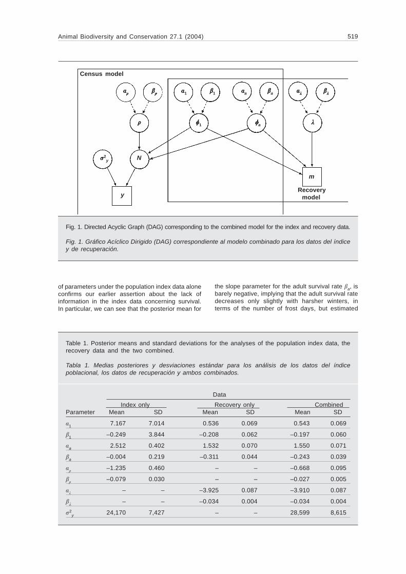
It is clear that both of these models have param-eters in common ( 1 and a). Thus, combining thetwo datasets and analysing them together pools theinformation regarding these parameters and thisfilters into the estimation of the remaining param-eters. The combination of these two models is mostclearly demonstrated in the Directed Acyclic Graph(DAG) given in figure 1.

In the DAG, known quantities (i.e., data) arerepresented by squares and unknown quantities(parameters to be estimated) by circles. Arrowsbetween nodes in the graph represent dependen-cies within the model between the correspondingnodes. Continuous arrows denote stochastic depend-encies such as those given in Equations (1)–(3), whilstdashed arrows denote deterministic dependenciessuch as those described in Equations (4)–(7). Ana-lysing the combined data simply involves mergingthe two individual DAG’s.

Similarly, and under the assumption of inde-pendence between the two data sources, we nowobtain a corresponding joint probability distributionfor the combined data as follows

ƒ (y, m* , , 1, a, Na, N1)

= ƒ(y* , 1, a, Na, N1) ƒ(m* , a, 1)

This is our basis for inference. From the classi-cal perspective, we treat this as a likelihood func-tion for the model parameters given the data andseek to maximise it with respect to those param-eters. The underlying population levels N1 and Naare essentially nuisance parameters which, ideally,we would like to integrate out of the likelihood.Unfortunately, this is impossible to do analyticallyand we need to adopt numerical techniques suchas the Kalman filter in order to obtain classicalestimates. Besbeas et al. (2002) provide a detaileddescription of the classical analysis.

From the Bayesian perspective, we elicit priorsfor the model parameters and combine these withthe joint probability density above to obtain a pos-terior density via Bayes’ theorem. The nuisanceparameters are then integrated out using MCMC.Several recent papers (Brooks et al., 2002; Dupuiset al., 2002; He et al., 2001; McAllister et al., 1994)discuss the application of Bayesian statistical meth-ods to parameter estimation for ecological modelsand many use the WinBUGS package (see e.g.,Link et al., 2002; Meyer & Millar, 1999) to carry outtheir analyses. We provide the correspondingWinBUGS code for our analyses in the appendix.

Analysis and results

We begin by specifying priors for our model param-eters. In some cases we might have prior informa-tion that we want to include e.g., relating to produc-tivity. Others who have analysed census or popula-tion index data alone from a Bayesian perspectivehave used informed priors (see e.g., Millar & Meyer,2000; Thomas et al., 2004). In other cases, forinstance with regard to regression coefficients, wemay know very little about what to expect. In thispaper we choose relatively vague priors to reflectthis uncertainty. Hence we take N(0,100) priors forthe regression parameters and an inverse gammaprior with parameters 0.001 for 2

y. We also need toplace priors on the initial population levels N1,2 andNa,2 (recall that our population index data begins inyear 3, within our parameterisation). Again, we takevague Normal priors with mean 200 and 1,000respectively and variances of 106 in order to avoidinfluencing the posterior with overly restrictive priors.An extensive sensitivity study in which each of theseprior parameter values were increased by severalorders of magnitude, gave essentially identical re-sults, suggesting that the exact choice of prior hadlittle influence on the results obtained.

We ran our MCMC algorithm for one millioniterations, discarding the first 100,000 as burn–inand thinning the remainder to one in every tenthobservation to save storage space. In general, theselection of starting points should have no affect onthe performance of the simulation nor on the finalresults. However, WinBUGS can occasionally getstuck or crash when certain starting point values areused. Posterior means often provide sensible start-ing values, though these would not generally beavailable in practice. MLE’s also provide suitablestarting points for analyses in WinBUGS. The analy-sis of the combined data set took approximately 18hours on a 850 MHz personal computer in WinBUGS,and we return to discuss the topic of computationaloverheads in "Discussion" section of the paper.

Table 1 provides the posterior means and corre-sponding standard deviations for the model param-eters from the analysis of the combined data, to-gether with the same estimates under the analysesof the two data sets individually. The comparativelylarge posterior standard deviations for the majority


Fig. 1. Directed Acyclic Graph (DAG) corresponding to the combined model for the index and recovery data.

Fig. 1. Gráfico Acíclico Dirigido (DAG) correspondiente al modelo combinado para los datos del índicey de recuperación.

Table 1. Posterior means and standard deviations for the analyses of the population index data, therecovery data and the two combined.

Tabla 1. Medias posteriores y desviaciones estándar para los análisis de los datos del índicepoblacional, los datos de recuperación y ambos combinados.

Data

Index only Recovery only Combined Parameter Mean SD Mean SD Mean SD

1 7.167 7.014 0.536 0.069 0.543 0.069

1 –0.249 3.844 –0.208 0.062 –0.197 0.060

a 2.512 0.402 1.532 0.070 1.550 0.071

a –0.004 0.219 –0.311 0.044 –0.243 0.039

–1.235 0.460 – – –0.668 0.095

–0.079 0.030 – – –0.027 0.005

– – –3.925 0.087 –3.910 0.087

– – –0.034 0.004 –0.034 0.004

2y 24,170 7,427 – – 28,599 8,615

of parameters under the population index data aloneconfirms our earlier assertion about the lack ofinformation in the index data concerning survival.In particular, we can see that the posterior mean for

the slope parameter for the adult survival rate a, isbarely negative, implying that the adult survival ratedecreases only slightly with harsher winters, interms of the number of frost days, but estimated

1 1 a a

1 a

2y N

m

y

Census model

Recovery model

520 Brooks et al.

with low precision. The posterior distribution forthe first year survival rate also has a large vari-ance, although the posterior mean for 1 is nega-tive. We note also the similarity in the parameterestimates under the ring–recovery model and thecombined analysis as in this application, it is thering–recovery data that provide most of the infor-mation about survival. Finally, we note that bycombining the two data sources, the posteriorstandard deviations for the productivity param-eters decrease dramatically, because of the addi-tional information about survival provided by therecovery data (table 2).

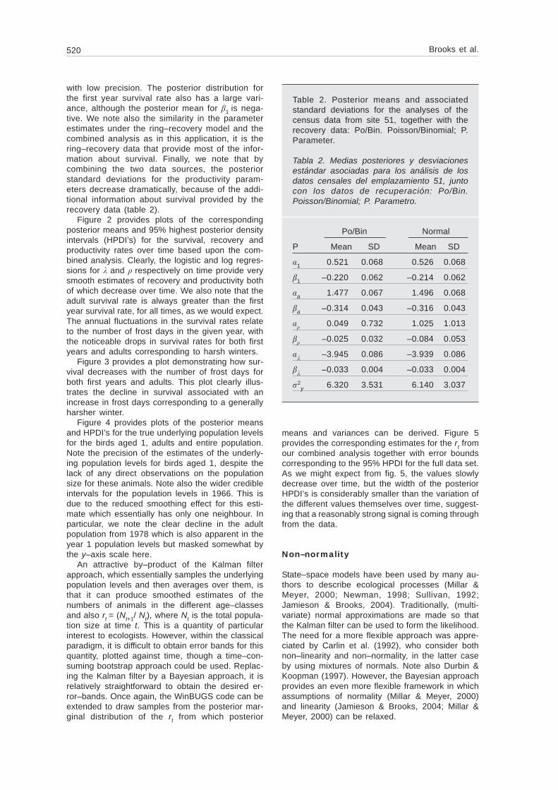
Figure 2 provides plots of the correspondingposterior means and 95% highest posterior densityintervals (HPDI’s) for the survival, recovery andproductivity rates over time based upon the com-bined analysis. Clearly, the logistic and log regres-sions for and respectively on time provide verysmooth estimates of recovery and productivity bothof which decrease over time. We also note that theadult survival rate is always greater than the firstyear survival rate, for all times, as we would expect.The annual fluctuations in the survival rates relateto the number of frost days in the given year, withthe noticeable drops in survival rates for both firstyears and adults corresponding to harsh winters.

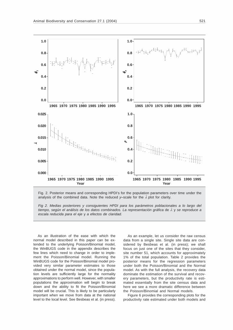
Figure 3 provides a plot demonstrating how sur-vival decreases with the number of frost days forboth first years and adults. This plot clearly illus-trates the decline in survival associated with anincrease in frost days corresponding to a generallyharsher winter.

Figure 4 provides plots of the posterior meansand HPDI’s for the true underlying population levelsfor the birds aged 1, adults and entire population.Note the precision of the estimates of the underly-ing population levels for birds aged 1, despite thelack of any direct observations on the populationsize for these animals. Note also the wider credibleintervals for the population levels in 1966. This isdue to the reduced smoothing effect for this esti-mate which essentially has only one neighbour. Inparticular, we note the clear decline in the adultpopulation from 1978 which is also apparent in theyear 1 population levels but masked somewhat bythe y–axis scale here.

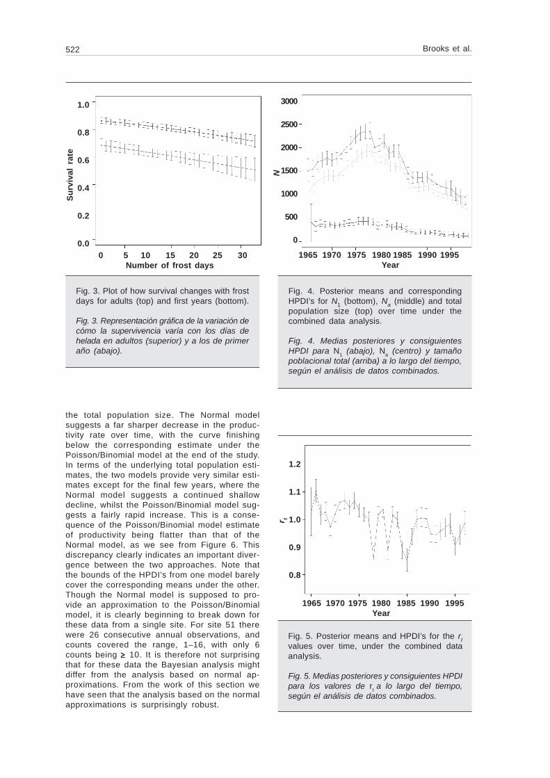
An attractive by–product of the Kalman filterapproach, which essentially samples the underlyingpopulation levels and then averages over them, isthat it can produce smoothed estimates of thenumbers of animals in the different age–classesand also rt = (Nt+1/ Nt), where Nt is the total popula-tion size at time t. This is a quantity of particularinterest to ecologists. However, within the classicalparadigm, it is difficult to obtain error bands for thisquantity, plotted against time, though a time–con-suming bootstrap approach could be used. Replac-ing the Kalman filter by a Bayesian approach, it isrelatively straightforward to obtain the desired er-ror–bands. Once again, the WinBUGS code can beextended to draw samples from the posterior mar-ginal distribution of the rt from which posterior

means and variances can be derived. Figure 5provides the corresponding estimates for the rt fromour combined analysis together with error boundscorresponding to the 95% HPDI for the full data set.As we might expect from fig. 5, the values slowlydecrease over time, but the width of the posteriorHPDI’s is considerably smaller than the variation ofthe different values themselves over time, suggest-ing that a reasonably strong signal is coming throughfrom the data.

Non–normality

State–space models have been used by many au-thors to describe ecological processes (Millar &Meyer, 2000; Newman, 1998; Sullivan, 1992;Jamieson & Brooks, 2004). Traditionally, (multi-variate) normal approximations are made so thatthe Kalman filter can be used to form the likelihood.The need for a more flexible approach was appre-ciated by Carlin et al. (1992), who consider bothnon–linearity and non–normality, in the latter caseby using mixtures of normals. Note also Durbin &Koopman (1997). However, the Bayesian approachprovides an even more flexible framework in whichassumptions of normality (Millar & Meyer, 2000)and linearity (Jamieson & Brooks, 2004; Millar &Meyer, 2000) can be relaxed.

Table 2. Posterior means and associatedstandard deviations for the analyses of thecensus data from site 51, together with therecovery data: Po/Bin. Poisson/Binomial; P.Parameter.

Tabla 2. Medias posteriores y desviacionesestándar asociadas para los análisis de losdatos censales del emplazamiento 51, juntocon los datos de recuperación: Po/Bin.Poisson/Binomial; P. Parametro.

Po/Bin Normal

P Mean SD Mean SD

1 0.521 0.068 0.526 0.068

1 –0.220 0.062 –0.214 0.062

a 1.477 0.067 1.496 0.068

a –0.314 0.043 –0.316 0.043

0.049 0.732 1.025 1.013

–0.025 0.032 –0.084 0.053

–3.945 0.086 –3.939 0.086

–0.033 0.004 –0.033 0.004

2y 6.320 3.531 6.140 3.037


Fig. 2. Posterior means and corresponding HPDI’s for the population parameters over time under theanalysis of the combined data. Note the reduced y–scale for the plot for clarity.

Fig 2. Medias posteriores y consiguientes HPDI para los parámetros poblacionales a lo largo deltiempo, según el análisis de los datos combinados. La representación gráfica de y se reproduce aescala reducida para el eje y a efectos de claridad.

1.0

0.8

0.6

0.4

0.2

0.0

1.0

0.8

0.6

0.4

0.2

0.0

1.0

0.8

0.6

0.4

0.2

0.0

0.025

0.020

0.015

0.010

0.005

0.000

1965 1970 1975 1980 1985 1990 1995 1965 1970 1975 1980 1985 1990 1995

1965 1970 1975 1980 1985 1990 1995 1965 1970 1975 1980 1985 1990 1995Year Year

1 a

As an illustration of the ease with which thenormal model described in this paper can be ex-tended to the underlying Poisson/Binomial model,the WinBUGS code in the appendix describes thefew lines which need to change in order to imple-ment the Poisson/Binomial model. Running theWinBUGS code for the Poisson/Binomial model pro-vided very similar parameter estimates to thoseobtained under the normal model, since the popula-tion levels are sufficiently large for the normalityapproximations to perform well. However, with smallerpopulations the approximation will begin to breakdown and the ability to fit the Poisson/Binomialmodel will be crucial. This is likely to be particularlyimportant when we move from data at the nationallevel to the local level. See Besbeas et al. (in press).

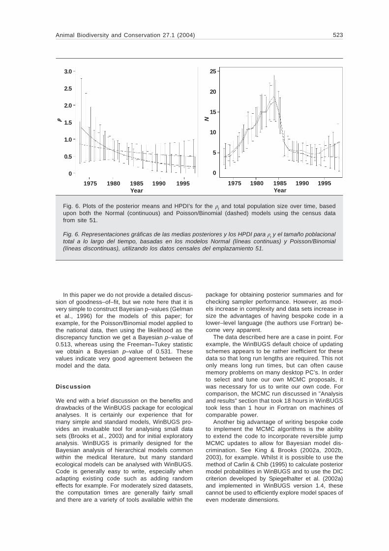
As an example, let us consider the raw censusdata from a single site. Single site data are con-sidered by Besbeas et al. (in press); we shallfocus on just one of the sites that they consider,site number 51, which accounts for approximately1% of the total population. Table 2 provides theposterior means for the regression parametersunder both the Poisson/Binomial and the Normalmodel. As with the full analysis, the recovery datadominate the estimation of the survival and recov-ery parameters, but the productivity rate is esti-mated essentially from the site census data andhere we see a more dramatic difference betweenthe Poisson/Binomial and Normal models.

Figure 6 provides the corresponding plots for theproductivity rate estimated under both models and

522 Brooks et al.

Fig. 5. Posterior means and HPDI’s for the rtvalues over time, under the combined dataanalysis.

Fig. 5. Medias posteriores y consiguientes HPDIpara los valores de rt a lo largo del tiempo,según el análisis de datos combinados.

1.2

1.1

1.0

0.9

0.8

1965 1970 1975 1980 1985 1990 1995Year

r tFig. 3. Plot of how survival changes with frostdays for adults (top) and first years (bottom).

Fig. 3. Representación gráfica de la variación decómo la supervivencia varía con los días dehelada en adultos (superior) y a los de primeraño (abajo).

Fig. 4. Posterior means and correspondingHPDI’s for N1 (bottom), Na (middle) and totalpopulation size (top) over time under thecombined data analysis.

Fig. 4. Medias posteriores y consiguientesHPDI para N1 (abajo), Na (centro) y tamañopoblacional total (arriba) a lo largo del tiempo,según el análisis de datos combinados.

the total population size. The Normal modelsuggests a far sharper decrease in the produc-tivity rate over time, with the curve finishingbelow the corresponding estimate under thePoisson/Binomial model at the end of the study.In terms of the underlying total population esti-mates, the two models provide very similar esti-mates except for the final few years, where theNormal model suggests a continued shallowdecline, whilst the Poisson/Binomial model sug-gests a fairly rapid increase. This is a conse-quence of the Poisson/Binomial model estimateof productivity being flatter than that of theNormal model, as we see from Figure 6. Thisdiscrepancy clearly indicates an important diver-gence between the two approaches. Note thatthe bounds of the HPDI’s from one model barelycover the corresponding means under the other.Though the Normal model is supposed to pro-vide an approximation to the Poisson/Binomialmodel, it is clearly beginning to break down forthese data from a single site. For site 51 therewere 26 consecutive annual observations, andcounts covered the range, 1–16, with only 6counts being $$$$$ 10. It is therefore not surprisingthat for these data the Bayesian analysis mightdiffer from the analysis based on normal ap-proximations. From the work of this section wehave seen that the analysis based on the normalapproximations is surprisingly robust.

1.0

0.8

0.6

0.4

0.2

0.01965 1970 1975 1980 1985 1990 1995

Year

3000

2500

2000

1500

1000

500

0

N

Su

rviv

al r

ate

0 5 10 15 20 25 30Number of frost days


In this paper we do not provide a detailed discus-sion of goodness–of–fit, but we note here that it isvery simple to construct Bayesian p–values (Gelmanet al., 1996) for the models of this paper; forexample, for the Poisson/Binomial model applied tothe national data, then using the likelihood as thediscrepancy function we get a Bayesian p–value of0.513, whereas using the Freeman–Tukey statisticwe obtain a Bayesian p–value of 0.531. Thesevalues indicate very good agreement between themodel and the data.

Discussion

We end with a brief discussion on the benefits anddrawbacks of the WinBUGS package for ecologicalanalyses. It is certainly our experience that formany simple and standard models, WinBUGS pro-vides an invaluable tool for analysing small datasets (Brooks et al., 2003) and for initial exploratoryanalysis. WinBUGS is primarily designed for theBayesian analysis of hierarchical models commonwithin the medical literature, but many standardecological models can be analysed with WinBUGS.Code is generally easy to write, especially whenadapting existing code such as adding randomeffects for example. For moderately sized datasets,the computation times are generally fairly smalland there are a variety of tools available within the

Fig. 6. Plots of the posterior means and HPDI’s for the t and total population size over time, basedupon both the Normal (continuous) and Poisson/Binomial (dashed) models using the census datafrom site 51.

Fig. 6. Representaciones gráficas de las medias posteriores y los HPDI para t y el tamaño poblacionaltotal a lo largo del tiempo, basadas en los modelos Normal (líneas continuas) y Poisson/Binomial(líneas discontinuas), utilizando los datos censales del emplazamiento 51.

1975 1980 1985 1990 1995Year

1975 1980 1985 1990 1995Year

3.0

2.5

2.0

1.5

1.0

0.5

0

N

25

20

15

10

5

0

package for obtaining posterior summaries and forchecking sampler performance. However, as mod-els increase in complexity and data sets increase insize the advantages of having bespoke code in alower–level language (the authors use Fortran) be-come very apparent.

The data described here are a case in point. Forexample, the WinBUGS default choice of updatingschemes appears to be rather inefficient for thesedata so that long run lengths are required. This notonly means long run times, but can often causememory problems on many desktop PC’s. In orderto select and tune our own MCMC proposals, itwas necessary for us to write our own code. Forcomparison, the MCMC run discussed in "Analysisand results" section that took 18 hours in WinBUGStook less than 1 hour in Fortran on machines ofcomparable power.

Another big advantage of writing bespoke codeto implement the MCMC algorithms is the abilityto extend the code to incorporate reversible jumpMCMC updates to allow for Bayesian model dis-crimination. See King & Brooks (2002a, 2002b,2003), for example. Whilst it is possible to use themethod of Carlin & Chib (1995) to calculate posteriormodel probabilities in WinBUGS and to use the DICcriterion developed by Spiegelhalter et al. (2002a)and implemented in WinBUGS version 1.4, thesecannot be used to efficiently explore model spaces ofeven moderate dimensions.

524 Brooks et al.

With any MCMC simulation, it is important tocheck convergence of the sampled values to theirstationary distribution. WinBUGS incorporates theso–called Brooks–Gelman–Rubin Diagnostic(Gelman & Rubin, 1992; Brooks & Gelman, 1998)and also allows for sampler output to be written toa file for analysis outside of the WinBUGS pack-age. The authors’ preferred method is to use stand-ard diagnostic techniques (Brooks & Roberts, 1998)to determine the burn–in length and then discardten times as many iterations as indicated. Severalreplications are run and compared and, if all agree,then convergence is assumed. However, the run–times within the WinBUGS package, coupled withthe inability to improve mixing by controlling pro-posal schemes can mean that this over–cautiousapproach cannot easily be followed in WinBUGS.Indeed the built–in diagnostics in WinBUGS ap-peared to diagnose convergence after just 100,000iterations, for the population index data alone thoughthe answers obtained from the longer run–lengthsadopted in this paper differ considerably from thoseobtained with such a short run (e.g., 1= –5.41; cftable 1). This problem is, of course, somewhatanalogous to the problems encountered in classicaloptimisation routines used to find maximum likeli-hood estimates where it is difficult to check that thetrue maximum has indeed been found. Overall,more experienced MCMC users are likely to benefitfrom developing their own suite of lower–level codesto implement their own MCMC algorithms. How-ever, as a tool for getting started, for performingexploratory analyses on moderately–sized datasetsand for teaching, the WinBUGS package is invalu-able (see the annex).

Acknowledgements

We thank the British Trust for Ornithology forpermission to use and present the population in-dex data for lapwings, and for providing the ring-recovery data. We also thank the BTO for provid-ing access to the individual site census data, andwe also gratefully acknowledge the work of themany BTO volunteers, whose labour results in thedata analysed in this paper. We are grateful toStephen Freeman at the BTO for his discussion ofthe issues involved.

References

Baillie, S. R. & Green, R. E., 1987. The Importanceof Variation in Recovery Rates when EstimatingSurvival Rates from Ringing Recoveries. ActaOrnithologica, 23: 41–60.

Besbeas, P., Freeman, S. N. & Morgan, B. J. T. (inpress). The Potential of Integrated PopulationModelling. Australian and New Zealand Journalof Statistics.

Besbeas, P., Freeman, S. N. & Morgan, B. J. T. &Catchpole, E. A., 2001. Stochastic Models for

Animal Abundance and Demographic Data. Tech-nical report, University of Kent UKC/IMS/01/06.

– 2002. Integrating Mark–Recapture–Recoveryand census Data to Estimate Animal Abun-dance and Demographic Parameters. Biomet-rics, 58: 540–547.

Brooks, S. P., 1998. Markov Chain Monte CarloMethod and its Application. The Statistician, 47:69–100.

Brooks, S. P., Catchpole, E. A., Morgan, B. J. T. &Harris, M., 2002. Bayesian Methods for Analys-ing Ringing Data. Journal of Applied Statistics,29: 187–206.

Brooks, S. P. & Gelman, A., 1998. Alternative Meth-ods for Monitoring Convergence of IterativeSimulations. Journal of Computational andGraphical Statistics, 7: 434–455.

Brooks, S. P., King, R. & Morgan, B. J. T., 2003.Bayesian Computation for Population Ecology.Technical Report 2003–11, Statistical Labora-tory, Univ. of Cambridge.

Brooks, S. P. & Roberts, G. O., 1998. DiagnosingConvergence of Markov Chain Monte Carlo Algo-rithms. Statistics and Computing, 8: 319–335.

Carlin, B. P. & Chib, S., 1995. Bayesian Model choicevia Markov Chain Monte Carlo. Journal of theRoyal Statistical Society, Series B 5: 473–484.

Carlin, B. P., Polson, N. G. & Stoffer, D. S., 1992. AMonte Carlo Approach to Nonnormal andNonlinear State–Space Modelling. Journal of theAmerican Statistical Association, 87: 493–500.

Catchpole, E. A., Freeman, S. N., Morgan, B. J. T.& Harris, M. P., 1998. Integrated recovery/recap-ture data analysis. Biometrics, 54: 33–46.

Dupuis, J., Badia, J., Maublanc, M.–L. & Bon, R.,2002. Survival and Spatial Fidelity of Mouflon(Ovis gmelini): a Bayesian Analysis of an Age–dependent Capture–Recapture Model. Journal ofAgricultural, Biological and Environmental Statis-tics, 7: 277–298.

Durbin, J. & Koopman, S. J., 1997. Monte CarloMaximum Likelihood Estimation for non–Gaussian State Space Models. Biometrika, 84:669–684.

Gamerman, D., 1995. Monte Carlo Markov Chainsfor Dynamic Generalised Linear Models. Techni-cal report. Univ. Federal do Rio de Janeiro,Brazil.

Gelman, A., Meng, X. & Stern, H., 1996. PosteriorPredictive Assessment of Model Fitness via Re-alized Discrepancies – with discussion. StatisticaSinica, 6.

Gelman, A. & Rubin, D. B., 1992. Inference fromIterative Simulation using Multiple Sequences.Statistical Science, 7: 457–511.

Gentleman, R., 1997. A Review of BUGS: BayesianInference Using Gibbs Sampling. Chance, 10:48–51.

Gilks, W. R., Richardson, S. & Spiegelhalter, D. J.,1996. Markov Chain Monte Carlo in Practice.Chapman and Hall.

He, C. Z., Sun, D. & Tra, Y. , 2001. BayesianModelling of Age–specific Survival in Nestling


Studies under Dirichlet Priors. Biometrics, 57:1059–1067.

Jamieson, L. E. & Brooks, S. P., 2004. DensityDependence in North American Ducks. AnimalBiodiversity and Conservation, 27.1: 113–128.

King, R. & Brooks, S. P., 2002a. Bayesian ModelDiscrimination for Multiple Strata Capture–Re-capture Data. Biometrika, 89: 785–806.

– 2002b. Model Selection for Integrated Recovery/Recapture Data. Biometrics, 58: 841–851.

– 2003. Investigating the Effect of Location, Ageand Sex on the Survival and Spatial Fidelity ofMouflon. Journal of Agricultural, Biological andEnvironmental Statistics, 8: 486–513.

King, R., Brooks, S. P., Mazzetta, C. & Freeman, S.N., 2004. Identifying and Diagnosing PopulationDeclines: A Bayesian Assessment of Lapwings inthe U.K. Technical Report, University of St. An-drews.

Link, W. A., Cam, E., Nichols, J. D. & Cooch,E. G., 2002. Of BUGS and Birds: Markov chainMonte Carlo for Hierarchical Modelling in Wild-life Research. Journal of Wildlife Management,66: 277–291.

McAllister, M. K., Pikitch, E. K., Punt, A. E. & Hilborn,R., 1994. A Bayesian Approach to Stock Assess-ment and Harvest Decisions Using the Sam-pling/Importance Resampling Algorithm. Cana-dian Journal of Fisheries and Aquatic Science,51: 2673–2687.

Meyer, R. & Millar, R. B., 1999. BUGS in BayesianStock Assessments. Canadian Journal of Fisher-

ies and Aquatic Science, 56: 1078–1086.Millar, R. B. & Meyer, R., 2000. Non–linear State

Space Modelling of Fisheries Biomass Dynam-ics by Using Metropolis–Hastings within–GibbsSampling. Applied Statistics, 49: 327–342.

Newman, K. B., 1998. State Space Modelling ofAnimal Movement and Mortality with Applica-tions to Salmon. Biometrics, 54: 1290–1314.

Spiegelhalter, D. J., Best, N. G., Carlin, B. P. &Van der Linde, A., 2002a. Bayesian Measures ofModel Complexity and Fit (with discussion). Jour-nal of the Royal Statistical Society, Series B, 64:583–639.

Spiegelhalter, D. J., Thomas, A. & Best, N. G..,2002b. WinBUGS User Manual, Version 1.4.MRC Biostatistics Unit, Cambridge.

Sullivan, P., 1992. A Kalman Filter Approach to Catch–at–Length Analysis. Biometrics, 48: 237–257.

Ter Braak, C. J. F., Van Strein, A. J., Meyer, R. &Verstrael, T. J., 1994. Analysing of MonitoringData with Many Missing Values: Which method?In: Bird Numbers 1992. Distribution, Monitoringand Ecological Aspects: 663–673 (W. Hagemeijer& T. Verstrael, Eds.). Beek–Ubbergeon, Sovon.

Thomas, L., Buckland, S. T., Newman, K. B. &Harwood, J., in press. A Unified Framework forModelling Wildlife Population Dynamics. Austral-ian and New Zealand Journal of Statistics.

Tucker, G. M., Davies, S. M. & Fuller, R. J., 1994. TheEcology and Conservation of Lapwings, Vanellusvanellus. Peterborough, Joint Nature ConservationCommittee (UK Nature Conservation), 9..

526 Brooks et al.

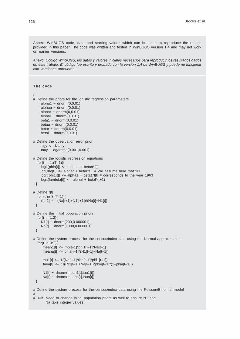
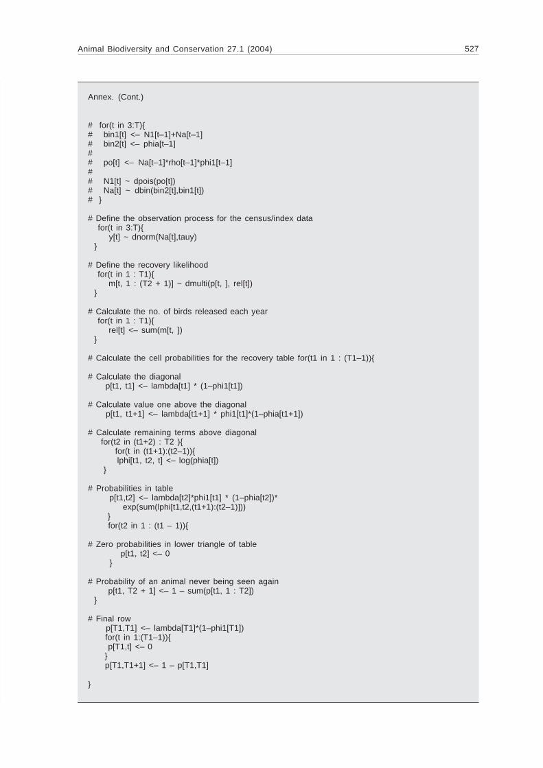
Annex. WinBUGS code, data and starting values which can be used to reproduce the resultsprovided in this paper. The code was written and tested in WinBUGS version 1.4 and may not workon earlier versions.

Anexo. Código WinBUGS, los datos y valores iniciales necesarios para reproducir los resultados dadosen este trabajo. El código fue escrito y probado con la versión 1.4 de WinBUGS y puede no funcionarcon versiones anteriores.

The code

{# Define the priors for the logistic regression parameters

alpha1 ~ dnorm(0,0.01) alphaa ~ dnorm(0,0.01) alphar ~ dnorm(0,0.01) alphal ~ dnorm(0,0.01) beta1 ~ dnorm(0,0.01) betaa ~ dnorm(0,0.01) betar ~ dnorm(0,0.01) betal ~ dnorm(0,0.01)

# Define the observation error prior sigy <– 1/tauy tauy ~ dgamma(0.001,0.001)

# Define the logistic regression equations for(t in 1:(T–1)){

logit(phia[t]) <– alphaa + betaa*f[t] log(rho[t]) <– alphar + betar*t # We assume here that t=1 logit(phi1[t]) <– alpha1 + beta1*f[t] # corresponds to the year 1963 logit(lambda[t]) <– alphal + betal*(t+1)

}

# Define r[t] for (t in 3:(T–1)){

r[t–2] <– (Na[t+1]+N1[t+1])/(Na[t]+N1[t]) }

# Define the initial population priors for(t in 1:2){

N1[t] ~ dnorm(200,0.000001) Na[t] ~ dnorm(1000,0.000001)

}

# Define the system process for the census/index data using the Normal approximation for(t in 3:T){

mean1[t] <– rho[t–1]*phi1[t–1]*Na[t–1] meana[t] <– phia[t–1]*(N1[t–1]+Na[t–1])

tau1[t] <– 1/(Na[t–1]*rho[t–1]*phi1[t–1]) taua[t] <– 1/((N1[t–1]+Na[t–1])*phia[t–1]*(1–phia[t–1]))

N1[t] ~ dnorm(mean1[t],tau1[t]) Na[t] ~ dnorm(meana[t],taua[t])

}

# Define the system process for the census/index data using the Poisson/Binomial model## NB. Need to change initial population priors as well to ensure N1 and Na take integer values


# for(t in 3:T){# bin1[t] <– N1[t–1]+Na[t–1]# bin2[t] <– phia[t–1]## po[t] <– Na[t–1]*rho[t–1]*phi1[t–1]## N1[t] ~ dpois(po[t])# Na[t] ~ dbin(bin2[t],bin1[t])# }

# Define the observation process for the census/index data for(t in 3:T){

y[t] ~ dnorm(Na[t],tauy) }

# Define the recovery likelihood for(t in 1 : T1){

m[t, 1 : (T2 + 1)] ~ dmulti(p[t, ], rel[t]) }

# Calculate the no. of birds released each year for(t in 1 : T1){

rel[t] <– sum(m[t, ]) }

# Calculate the cell probabilities for the recovery table for(t1 in 1 : (T1–1)){

# Calculate the diagonal p[t1, t1] <– lambda[t1] * (1–phi1[t1])

# Calculate value one above the diagonal p[t1, t1+1] <– lambda[t1+1] * phi1[t1]*(1–phia[t1+1])

# Calculate remaining terms above diagonal for(t2 in (t1+2) : T2 ){

for(t in (t1+1):(t2–1)){ lphi[t1, t2, t] <– log(phia[t])}

# Probabilities in table p[t1,t2] <– lambda[t2]*phi1[t1] * (1–phia[t2])* exp(sum(lphi[t1,t2,(t1+1):(t2–1)])) } for(t2 in 1 : (t1 – 1)){

# Zero probabilities in lower triangle of table p[t1, t2] <– 0

}

# Probability of an animal never being seen again p[t1, T2 + 1] <– 1 – sum(p[t1, 1 : T2])

}

# Final row p[T1,T1] <– lambda[T1]*(1–phi1[T1]) for(t in 1:(T1–1)){ p[T1,t] <– 0 } p[T1,T1+1] <– 1 – p[T1,T1]

}

Annex. (Cont.)

528 Brooks et al.

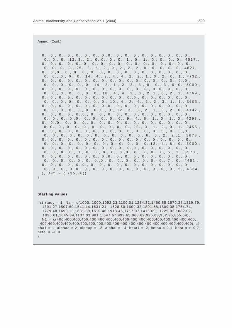
Data

The data here correspond to index records from 1965 to 1998, (normalised) frost days from 1963 to1997 and recovery data from 1963 to 1997. Zeroes are added to make all data run from 1963 until1998.

list (T = 36, y = c (0,0, 1092.23,1 100.01, 1234.32, 1460.85, 1570.38, 1819.79,1391.27,1507.60, 1541.44,1631.21,1628.60,1609.33,1801.68,1809.08,1754.74,1779.48,1699.13, 1681.39,1610.46,1918.45,1717.07,1415.69,1229.02,1082.02,1096.61,1045.84, 11 3 7 . 0 3 , 9 8 1 . 1 , 6 4 7 . 6 7 , 9 9 2 . 6 5 , 9 6 8 . 6 2 , 9 2 6 . 8 3 , 9 5 2 . 9 6 , 8 6 5 . 6 4 ) , f = c (0 .1922 ,0 .3082 ,0 .3082 ,–0 .9676 ,0 .5401 ,0 .3082 ,1 .1995 ,0 .1921 ,–0 .8526 , –1 .0835 ,–0 .6196 ,–1 .1995 ,–0 .5037 ,–0 .1557 ,0 .0762 ,2 .628 ,–0 .3877 ,–0 .968 , 1 . 9318 ,–0 .6196 ,–0 .3877 ,1 .700 , 2 .2797 ,0 .6561 ,–0 .8516 ,–1 .0835 ,–1 .0835 , 0 . 1 9 2 2 , 0 . 1 9 2 2 , – 0 . 1 5 5 7 , – 0 . 5 0 3 7 , – 0 . 8 5 1 6 , 0 . 8 8 8 0 , – 0 . 0 3 9 8 , – 1 . 1 9 9 5 , 0 ) , T1 = 35, T2 = 35, m = structure(. Data = c( 1 3 . , 4 . , 1 . , 2 . , 1 . , 0 . , 0 . , 1 . , 0 . , 0 . , 0 . , 1 . , 0 . , 0 . , 0 . , 0 . , 0 . , 0 . , 0 . , 0 . , 0 . , 0 . , 0 . , 0 . , 0 . , 0 . , 0 . , 0 . , 0 . , 0 . , 0 . , 0 . , 0 . , 0 . , 0 . , 1 1 2 4 . , 0 . , 1 6 . , 4 . , 3 . , 0 . , 1 . , 1 . , 0 . , 0 . , 0 . , 0 . , 0 . , 1 . , 0 . , 0 . , 0 . , 0 . , 0 . , 0 . , 0 . , 0 . , 0 . , 0 . , 0 . , 0 . , 0 . , 0 . , 0 . , 0 . , 0 . , 0 . , 0 . , 0 . , 0 . , 0 . , 1 2 5 9 . , 0 . , 0 . , 1 1 . , 1 . , 1 . , 1 . , 0 . , 2 . , 1 . , 1 . , 1 . , 1 . , 2 . , 0 . , 0 . , 1 . , 0 . , 0 . , 1 . , 0 . , 0 . , 0 . , 0 . , 0 . , 0 . , 0 . , 0 . , 0 . , 0 . , 0 . , 0 . , 0 . , 0 . , 0 . , 0 . , 1 0 8 2 . , 0 . , 0 . , 0 . , 1 0 . , 4 . , 2 . , 1 . , 1 . , 1 . , 0 . , 0 . , 0 . , 0 . , 0 . , 0 . , 0 . , 1 . , 0 . , 0 . , 0 . , 0 . , 0 . , 0 . , 0 . , 0 . , 0 . , 0 . , 0 . , 0 . , 0 . , 0 . , 0 . , 0 . , 0 . , 0 . , 1 5 9 5 . , 0 . , 0 . , 0 . , 0 . , 1 1 . , 1 . , 5 . , 0 . , 0 . , 0 . , 1 . , 1 . , 1 . , 1 . , 1 . , 0 . , 0 . , 0 . , 0 . , 0 . , 0 . , 0 . , 0 . , 0 . , 0 . , 0 . , 0 . , 0 . , 0 . , 0 . , 0 . , 0 . , 0 . , 0 . , 0 . , 1 5 9 6 . , 0 . , 0 . , 0 . , 0 . , 0 . , 9 . , 5 . , 4 . , 0 . , 2 . , 2 . , 2 . , 1 . , 2 . , 0 . , 1 . , 0 . , 0 . , 1 . , 0 . , 0 . , 0 . , 0 . , 0 . , 0 . , 0 . , 0 . , 0 . , 0 . , 0 . , 0 . , 0 . , 0 . , 0 . , 0 . , 2 0 9 1 . , 0 . , 0 . , 0 . , 0 . , 0 . , 0 . , 1 1 . , 9 . , 4 . , 3 . , 1 . , 1 . , 1 . , 3 . , 2 . , 2 . , 1 . , 0 . , 0 . , 0 . , 0 . , 1 . , 0 . , 0 . , 0 . , 0 . , 0 . , 0 . , 0 . , 0 . , 0 . , 0 . , 0 . , 0 . , 0 . , 1 9 6 4 . , 0 . , 0 . , 0 . , 0 . , 0 . , 0 . , 0 . , 8 . , 4 . , 2 . , 0 . , 0 . , 0 . , 1 . , 2 . , 3 . , 0 . , 0 . , 0 . , 0 . , 0 . , 1 . , 0 . , 0 . , 0 . , 0 . , 0 . , 0 . , 0 . , 0 . , 0 . , 0 . , 0 . , 0 . , 0 . , 1 9 4 2 . , 0 . , 0 . , 0 . , 0 . , 0 . , 0 . , 0 . , 0 . , 4 . , 1 . , 1 . , 2 . , 2 . , 1 . , 3 . , 3 . , 0 . , 2 . , 0 . , 0 . , 0 . , 0 . , 0 . , 0 . , 0 . , 0 . , 0 . , 0 . , 0 . , 0 . , 0 . , 0 . , 0 . , 0 . , 0 . , 2 4 4 4 . , 0 . , 0 . , 0 . , 0 . , 0 . , 0 . , 0 . , 0 . , 0 . , 8 . , 2 . , 2 . , 2 . , 6 . , 1 . , 5 . , 2 . , 1 . , 3 . , 1 . , 1 . , 1 . , 2 . , 0 . , 0 . , 0 . , 0 . , 0 . , 0 . , 0 . , 0 . , 0 . , 0 . , 0 . , 0 . , 3 0 5 5 . , 0 . , 0 . , 0 . , 0 . , 0 . , 0 . , 0 . , 0 . , 0 . , 0 . , 1 6 . , 1 . , 1 . , 1 . , 2 . , 3 . , 2 . , 0 . , 1 . , 1 . , 1 . , 1 . , 0 . , 0 . , 0 . , 0 . , 0 . , 0 . , 0 . , 0 . , 0 . , 0 . , 0 . , 0 . , 0 . , 3 4 1 2 . , 0 . , 0 . , 0 . , 0 . , 0 . , 0 . , 0 . , 0 . , 0 . , 0 . , 0 . , 1 3 . , 4 . , 4 . , 7 . , 3 . , 1 . , 1 . , 1 . , 1 . , 0 . , 0 . , 2 . , 1 . , 0 . , 0 . , 0 . , 0 . , 0 . , 0 . , 0 . , 0 . , 0 . , 0 . , 0 . , 3 9 0 7 . , 0 . , 0 . , 0 . , 0 . , 0 . , 0 . , 0 . , 0 . , 0 . , 0 . , 0 . , 0 . , 1 1 . , 4 . , 0 . , 2 . , 1 . , 1 . , 2 . , 2 . , 0 . , 3 . , 0 . , 0 . , 0 . , 0 . , 0 . , 0 . , 0 . , 0 . , 0 . , 0 . , 0 . , 0 . , 0 . , 2 5 3 8 . , 0 . , 0 . , 0 . , 0 . , 0 . , 0 . , 0 . , 0 . , 0 . , 0 . , 0 . , 0 . , 0 . , 1 1 . , 3 . , 5 . , 1 . , 3 . , 3 . , 2 . , 3 . , 0 . , 1 . , 0 . , 1 . , 1 . , 0 . , 0 . , 0 . , 0 . , 0 . , 0 . , 0 . , 0 . , 0 . , 3 2 7 0 . , 0 . , 0 . , 0 . , 0 . , 0 . , 0 . , 0 . , 0 . , 0 . , 0 . , 0 . , 0 . , 0 . , 0 . , 1 2 . , 5 . , 0 . , 5 . , 4 . , 2 . , 1 . , 2 . , 3 . , 0 . , 0 . , 0 . , 1 . , 0 . , 0 . , 0 . , 0 . , 0 . , 0 . , 0 . , 0 . , 3 4 4 3 . , 0 . , 0 . , 0 . , 0 . , 0 . , 0 . , 0 . , 0 . , 0 . , 0 . , 0 . , 0 . , 0 . , 0 . , 0 . , 1 5 . , 5 . , 2 . , 2 . , 0 . , 5 . , 3 . , 0 . , 0 . , 0 . , 1 . , 0 . , 0 . , 0 . , 0 . , 0 . , 0 . , 0 . , 0 . , 0 . , 3 1 3 2 . , 0 . , 0 . , 0 . , 0 . , 0 . , 0 . , 0 . , 0 . , 0 . , 0 . , 0 . , 0 . , 0 . , 0 . , 0 . , 0 . , 7 . , 4 . , 6 . , 1 . , 3 . , 3 . , 2 . , 0 . , 1 . , 0 . , 0 . , 1 . , 0 . , 1 . , 0 . , 0 . , 0 . , 0 . , 0 . , 3 2 7 5 . , 0 . , 0 . , 0 . , 0 . , 0 . , 0 . , 0 . , 0 . , 0 . , 0 . , 0 . , 0 . , 0 . , 0 . , 0 . , 0 . , 0 . , 1 3 . , 8 . , 1 . , 2 . , 4 . , 5 . , 3 . , 0 . , 1 . , 2 . , 0 . , 0 . , 1 . , 0 . , 0 . , 0 . , 0 . , 0 . , 3 4 4 7 . , 0 . , 0 . , 0 . , 0 . , 0 . , 0 . , 0 . , 0 . , 0 . , 0 . , 0 . , 0 . , 0 . , 0 . , 0 . , 0 . , 0 . , 0 . , 2 3 . , 2 . , 2 . , 3 . , 3 . , 3 . , 1 . , 0 . , 0 . , 0 . , 0 . , 0 . , 0 . , 0 . , 0 . , 0 . , 0 . , 3 9 0 2 . , 0 . , 0 . , 0 . , 0 . , 0 . , 0 . , 0 . , 0 . , 0 . , 0 . , 0 . , 0 . , 0 . , 0 . , 0 . , 0 . , 0 . , 0 . , 0 . , 1 0 . , 0 . , 6 . , 2 . , 0 . , 1 . , 1 . , 0 . , 0 . , 1 . , 0 . , 0 . , 0 . , 0 . , 0 . , 0 . , 2 8 6 0 . , 0 . , 0 . , 0 . , 0 . , 0 . , 0 . , 0 . , 0 . , 0 . , 0 . , 0 . , 0 . , 0 . , 0 . , 0 . , 0 . , 0 . , 0 . , 0 . , 0 . , 1 9 . , 7 . , 6 . , 4 . , 0 . , 0 . , 2 . , 0 . , 0 . , 0 . , 1 . , 2 . , 0 . , 0 . , 1 . , 4 0 7 7 . ,

Annex. (Cont.)


0 . , 0 . , 0 . , 0 . , 0 . , 0 . , 0 . , 0 . , 0 . , 0 . , 0 . , 0 . , 0 . , 0 . , 0 . , 0 . , 0 . , 0 . , 0 . , 0 . , 0 . , 1 2 . , 3 . , 2 . , 0 . , 0 . , 0 . , 0 . , 1 . , 0 . , 1 . , 0 . , 0 . , 0 . , 0 . , 4 0 1 7 . , 0 . , 0 . , 0 . , 0 . , 0 . , 0 . , 0 . , 0 . , 0 . , 0 . , 0 . , 0 . , 0 . , 0 . , 0 . , 0 . , 0 . , 0 . , 0 . , 0 . , 0 . , 0 . , 2 5 . , 2 . , 5 . , 2 . , 0 . , 2 . , 2 . , 2 . , 0 . , 0 . , 0 . , 0 . , 0 . , 4 8 2 7 . , 0 . , 0 . , 0 . , 0 . , 0 . , 0 . , 0 . , 0 . , 0 . , 0 . , 0 . , 0 . , 0 . , 0 . , 0 . , 0 . , 0 . , 0 . , 0 . , 0 . , 0 . , 0 . , 0 . , 1 4 . , 4 . , 3 . , 4 . , 4 . , 2 . , 2 . , 1 . , 0 . , 2 . , 0 . , 1 . , 4 7 3 2 . , 0 . , 0 . , 0 . , 0 . , 0 . , 0 . , 0 . , 0 . , 0 . , 0 . , 0 . , 0 . , 0 . , 0 . , 0 . , 0 . , 0 . , 0 . , 0 . , 0 . , 0 . , 0 . , 0 . , 0 . , 1 4 . , 2 . , 1 . , 2 . , 2 . , 3 . , 0 . , 0 . , 3 . , 0 . , 0 . , 5 0 0 0 . , 0 . , 0 . , 0 . , 0 . , 0 . , 0 . , 0 . , 0 . , 0 . , 0 . , 0 . , 0 . , 0 . , 0 . , 0 . , 0 . , 0 . , 0 . , 0 . , 0 . , 0 . , 0 . , 0 . , 0 . , 0 . , 1 8 . , 4 . , 4 . , 3 . , 0 . , 2 . , 1 . , 0 . , 2 . , 1 . , 4 7 6 9 . , 0 . , 0 . , 0 . , 0 . , 0 . , 0 . , 0 . , 0 . , 0 . , 0 . , 0 . , 0 . , 0 . , 0 . , 0 . , 0 . , 0 . , 0 . , 0 . , 0 . , 0 . , 0 . , 0 . , 0 . , 0 . , 0 . , 1 0 . , 4 . , 2 . , 4 . , 2 . , 2 . , 3 . , 1 . , 1 . , 3 6 0 3 . , 0 . , 0 . , 0 . , 0 . , 0 . , 0 . , 0 . , 0 . , 0 . , 0 . , 0 . , 0 . , 0 . , 0 . , 0 . , 0 . , 0 . , 0 . , 0 . , 0 . , 0 . , 0 . , 0 . , 0 . , 0 . , 0 . , 0 . , 1 2 . , 3 . , 3 . , 2 . , 1 . , 0 . , 2 . , 0 . , 4 1 4 7 . , 0 . , 0 . , 0 . , 0 . , 0 . , 0 . , 0 . , 0 . , 0 . , 0 . , 0 . , 0 . , 0 . , 0 . , 0 . , 0 . , 0 . , 0 . , 0 . , 0 . , 0 . , 0 . , 0 . , 0 . , 0 . , 0 . , 0 . , 0 . , 9 . , 4 . , 6 . , 1 . , 0 . , 1 . , 0 . , 4 2 9 3 . , 0 . , 0 . , 0 . , 0 . , 0 . , 0 . , 0 . , 0 . , 0 . , 0 . , 0 . , 0 . , 0 . , 0 . , 0 . , 0 . , 0 . , 0 . , 0 . , 0 . , 0 . , 0 . , 0 . , 0 . , 0 . , 0 . , 0 . , 0 . , 0 . , 1 8 . , 3 . , 1 . , 2 . , 0 . , 1 . , 3 4 5 5 . , 0 . , 0 . , 0 . , 0 . , 0 . , 0 . , 0 . , 0 . , 0 . , 0 . , 0 . , 0 . , 0 . , 0 . , 0 . , 0 . , 0 . , 0 . , 0 . , 0 . , 0 . , 0 . , 0 . , 0 . , 0 . , 0 . , 0 . , 0 . , 0 . , 0 . , 6 . , 5 . , 2 . , 2 . , 1 . , 3 6 7 3 . , 0 . , 0 . , 0 . , 0 . , 0 . , 0 . , 0 . , 0 . , 0 . , 0 . , 0 . , 0 . , 0 . , 0 . , 0 . , 0 . , 0 . , 0 . , 0 . , 0 . , 0 . , 0 . , 0 . , 0 . , 0 . , 0 . , 0 . , 0 . , 0 . , 0 . , 0 . , 1 2 . , 4 . , 6 . , 0 . , 3 9 0 0 . , 0 . , 0 . , 0 . , 0 . , 0 . , 0 . , 0 . , 0 . , 0 . , 0 . , 0 . , 0 . , 0 . , 0 . , 0 . , 0 . , 0 . , 0 . , 0 . , 0 . , 0 . , 0 . , 0 . , 0 . , 0 . , 0 . , 0 . , 0 . , 0 . , 0 . , 0 . , 0 . , 7 . , 5 . , 1 . , 3 5 7 8 . , 0 . , 0 . , 0 . , 0 . , 0 . , 0 . , 0 . , 0 . , 0 . , 0 . , 0 . , 0 . , 0 . , 0 . , 0 . , 0 . , 0 . , 0 . , 0 . , 0 . , 0 . , 0 . , 0 . , 0 . , 0 . , 0 . , 0 . , 0 . , 0 . , 0 . , 0 . , 0 . , 0 . , 7 . , 0 . , 4 4 8 1 . , 0 . , 0 . , 0 . , 0 . , 0 . , 0 . , 0 . , 0 . , 0 . , 0 . , 0 . , 0 . , 0 . , 0 . , 0 . , 0 . , 0 . , 0 . , 0 . , 0 . , 0 . , 0 . , 0 . , 0 . , 0 . , 0 . , 0 . , 0 . , 0 . , 0 . , 0 . , 0 . , 0 . , 0 . , 5 . , 4 3 3 4 . ) , . D i m = c ( 3 5 , 3 6 ) ))

Starting values

l is t ( tauy = 1, Na = c(1000.,1000,1092.23,1100.01,1234.32,1460.85,1570.38,1819.79, 1391.27,1507.60,1541.44,1631.21, 1628.60,1609.33,1801.68,1809.08,1754.74, 1779.48,1699.13,1681.39,1610.46,1918.45,1717.07,1415.69, 1229.02,1082.02, 1096.61,1045.84,1137.03,981.1,647.67,992.65,968.62,926.83,952.96,865.64), N1 = c(400,400,400,400,400,400,400,400,400,400,400,400,400,400,400,400,400, 400,400,400,400,400,400,400,400,400,400,400,400,400,400,400,400,400,400,400), al-pha1 = 1, alphaa = 2, alphap = –2, alphal = –4, beta1 =–2, betaa = 0.1, beta p =–0.7,betal = –0.3)

Annex. (Cont.)

Documents

Animal Biodiversity and Conservation 27.1 (2004) A …abc.museucienciesjournals.cat/files/ABC-27-1-pp-515-529.pdf · Palabras clave: Datos de censo, Análisis integrado, Filtro de