Embed Size (px)
DESCRIPTION
ISSN: 1578-665 X An international journal devoted to the study and conservation of animal biodiversity
Citation preview

Form
erly
Mis
cel·l
ània
Zo
olò
gic
a
2001
AnimalBiodiversity Conservation24.1
an
d
Editor executiu / Editor ejecutivo / Executive EditorJoan Carles SenarJoan Carles SenarJoan Carles SenarJoan Carles SenarJoan Carles Senar
Secretària de Redacció / Secretaria de Redacción /Managing EditorMontserrat FerrerMontserrat FerrerMontserrat FerrerMontserrat FerrerMontserrat Ferrer
Consell Assessor / Consejo asesor / Advisory BoardOleguer EscolàOleguer EscolàOleguer EscolàOleguer EscolàOleguer EscolàEulàlia GarciaEulàlia GarciaEulàlia GarciaEulàlia GarciaEulàlia GarciaAnna OmedesAnna OmedesAnna OmedesAnna OmedesAnna OmedesJosep PiquéJosep PiquéJosep PiquéJosep PiquéJosep PiquéFrancesc UribeFrancesc UribeFrancesc UribeFrancesc UribeFrancesc Uribe
Editors / Editores / EditorsAntonio Barbadilla Antonio Barbadilla Antonio Barbadilla Antonio Barbadilla Antonio Barbadilla Univ. Autònoma de Barcelona, Bellaterra, SpainXavier BellésXavier BellésXavier BellésXavier BellésXavier Bellés Centre d' Investigació i Desenvolupament CSIC, Barcelona, SpainJuan Carranza Juan Carranza Juan Carranza Juan Carranza Juan Carranza Univ. de Extremadura, Cáceres, SpainLuís Mª CarrascalLuís Mª CarrascalLuís Mª CarrascalLuís Mª CarrascalLuís Mª Carrascal Museo Nacional de Ciencias Naturales CSIC, Madrid, SpainAdolfo Cordero Adolfo Cordero Adolfo Cordero Adolfo Cordero Adolfo Cordero Univ. de Vigo, Vigo, SpainMario Díaz Mario Díaz Mario Díaz Mario Díaz Mario Díaz Univ. de Castilla–La Mancha, Toledo, SpainXavier Domingo Xavier Domingo Xavier Domingo Xavier Domingo Xavier Domingo Univ. Pompeu Fabra, Barcelona, SpainFrancisco Palomares Francisco Palomares Francisco Palomares Francisco Palomares Francisco Palomares Estación Biológica de Doñana, Sevilla, SpainFrancesc Piferrer Francesc Piferrer Francesc Piferrer Francesc Piferrer Francesc Piferrer Inst. de Ciències del Mar CSIC, Barcelona, SpainIgnacio Ribera Ignacio Ribera Ignacio Ribera Ignacio Ribera Ignacio Ribera The Natural History Museum, London, United KingdomAlfredo Salvador Alfredo Salvador Alfredo Salvador Alfredo Salvador Alfredo Salvador Museo Nacional de Ciencias Naturales, Madrid, SpainJosé Luís TJosé Luís TJosé Luís TJosé Luís TJosé Luís Tellería ellería ellería ellería ellería Univ. Complutense de Madrid, Madrid, SpainFrancesc Uribe Francesc Uribe Francesc Uribe Francesc Uribe Francesc Uribe Museu de Zoologia de Barcelona, Barcelona, Spain
Consell Editor / Consejo editor / Editorial BoardJosé A. BarrientosJosé A. BarrientosJosé A. BarrientosJosé A. BarrientosJosé A. Barrientos Univ. Autònoma de Barcelona, Bellaterra, SpainJean C. BeaucournuJean C. BeaucournuJean C. BeaucournuJean C. BeaucournuJean C. Beaucournu Univ. de Rennes, Rennes, FranceDavid M. BirdDavid M. BirdDavid M. BirdDavid M. BirdDavid M. Bird McGill Univ., Québec, CanadaMats BjörklundMats BjörklundMats BjörklundMats BjörklundMats Björklund Uppsala Univ., Uppsala, SwedenJean BouillonJean BouillonJean BouillonJean BouillonJean Bouillon Univ. Libre de Bruxelles, Brussels, BelgiumMiguel Delibes Miguel Delibes Miguel Delibes Miguel Delibes Miguel Delibes Estación Biológica de Doñana CSIC, Sevilla, SpainDario J. Díaz CosínDario J. Díaz CosínDario J. Díaz CosínDario J. Díaz CosínDario J. Díaz Cosín Univ. Complutense de Madrid, Madrid, SpainAlain DuboisAlain DuboisAlain DuboisAlain DuboisAlain Dubois Museum national d’Histoire naturelle CNRS, Paris, FranceJohn FaJohn FaJohn FaJohn FaJohn Fa Durrell Wildlife Conservation Trust, Trinity, United KingdomMarco Festa–BianchetMarco Festa–BianchetMarco Festa–BianchetMarco Festa–BianchetMarco Festa–Bianchet Univ. de Sherbrooke, Québec, CanadaRosa FlosRosa FlosRosa FlosRosa FlosRosa Flos Univ. Politècnica de Catalunya, Barcelona, SpainJosep Mª GiliJosep Mª GiliJosep Mª GiliJosep Mª GiliJosep Mª Gili Inst. de Ciències del Mar CMIMA–CSIC, Barcelona, SpainEdmund Gittenberger Edmund Gittenberger Edmund Gittenberger Edmund Gittenberger Edmund Gittenberger Rijksmuseum van Natuurlijke Historie, Leiden, The NetherlandsFernando HiraldoFernando HiraldoFernando HiraldoFernando HiraldoFernando Hiraldo Estación Biológica de Doñana CSIC, Sevilla, SpainPatrick LavellePatrick LavellePatrick LavellePatrick LavellePatrick Lavelle Inst. Français de recherche scient. pour le develop. en cooperation, Bondy, FranceSantiago Mas–ComaSantiago Mas–ComaSantiago Mas–ComaSantiago Mas–ComaSantiago Mas–Coma Univ. de Valencia, Valencia, SpainJoaquín MateuJoaquín MateuJoaquín MateuJoaquín MateuJoaquín Mateu Estación Experimental de Zonas Áridas CSIC, Almería, SpainNeil MetcalfeNeil MetcalfeNeil MetcalfeNeil MetcalfeNeil Metcalfe Univ. of Glasgow, Glasgow, United KingdomJacint NadalJacint NadalJacint NadalJacint NadalJacint Nadal Univ. de Barcelona, Barcelona, SpainStewart B. PeckStewart B. PeckStewart B. PeckStewart B. PeckStewart B. Peck Carleton Univ., Ottawa, CanadaEduard PetitpierreEduard PetitpierreEduard PetitpierreEduard PetitpierreEduard Petitpierre Univ. de les Illes Balears, Palma de Mallorca, SpainTTTTTaylor H. Ricketts aylor H. Ricketts aylor H. Ricketts aylor H. Ricketts aylor H. Ricketts Stanford Univ., Stanford, USAJoandomènec RosJoandomènec RosJoandomènec RosJoandomènec RosJoandomènec Ros Univ. de Barcelona, Barcelona, SpainVVVVValentín Sans–Comaalentín Sans–Comaalentín Sans–Comaalentín Sans–Comaalentín Sans–Coma Univ. de Málaga, Málaga, SpainTTTTTore Slagsvoldore Slagsvoldore Slagsvoldore Slagsvoldore Slagsvold Univ. of Oslo, Oslo, Norway
Secretaria de Redacció / Secretaría de Redacción /Editorial Office
Museu de ZoologiaPasseig Picasso s/n08003 Barcelona, SpainTel. +34–93–3196912Fax +34–93–3104999E–mail [email protected]
"La tortue greque" Oeuvres du Comte de Lacépède comprenant L'Histoire Naturelle des Quadrupèdes Ovipares, desSerpents, des Poissons et des Cétacés; Nouvelle édition avec planches coloriées dirigée par M. A. G. Desmarest;Bruxelles: Th. Lejeuné, Éditeur des oeuvres de Buffon, 1836. Pl. 7
Animal Biodiversity and Conservation 24.1, 2001Animal Biodiversity and Conservation 24.1, 2001Animal Biodiversity and Conservation 24.1, 2001Animal Biodiversity and Conservation 24.1, 2001Animal Biodiversity and Conservation 24.1, 2001© 2001 Museu de Zoologia, Institut de Cultura, Ajuntament de BarcelonaAutoedició: Montserrat FerrerFotomecànica i impressió: Sociedad Cooperativa Librería GeneralISSN: 1578–665XDipòsit legal: B–16.278–58
1Animal Biodiversity and Conservation 24.1 (2001)
© 2001 Museu de ZoologiaISSN: 1578–665X
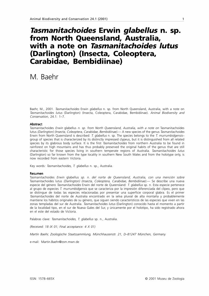
Tasmanitachoides Erwin glabellus n. sp.from North Queensland, Australia,with a note on Tasmanitachoides lutus(Darlington) (Insecta, Coleoptera,Carabidae, Bembidiinae)
M. Baehr
Baehr, M., 2001. Tasmanitachoides Erwin glabellus n. sp. from North Queensland, Australia, with a note onTasmanitachoides lutus (Darlington) (Insecta, Coleoptera, Carabidae, Bembidiinae). Animal Biodiversity andConservation, 24.1: 1–7.
AbstractAbstractAbstractAbstractAbstractTasmanitachoides Erwin glabellus n. sp. from North Queensland, Australia, with a note on Tasmanitachoideslutus (Darlington) (Insecta, Coleoptera, Carabidae, Bembidiinae).— A new species of the genus TasmanitachoidesErwin from North Queensland is described: T. glabellus n. sp. The species belongs to the T. murrumbidgensis–group of species that is characterized by its distinctly impressed clypeus, but it is distinguished from all relatedspecies by its glabrous body surface. It is the first Tasmanitachoides from northern Australia to be found inrainforest on high mountains and has thus probably preserved the original habits of the genus that are stillcharacteristic for those species living in southern temperate regions of Australia. Tasmanitachoides lutus(Darlington) so far known from the type locality in southern New South Wales and from the holotype only, isnow recorded from eastern Victoria.
Key words: Tasmanitachoides, T. glabellus n. sp., Australia.
ResumenResumenResumenResumenResumenTasmanitachoides Erwin glabellus sp. n. del norte de Queensland, Australia, con una mención sobreTasmanitachoides lutus (Darlington) (Insecta, Coleoptera, Carabidae, Bembidiinae).— Se describe una nuevaespecie del género Tasmanitachoides Erwin del norte de Queensland: T. glabellus sp. n. Esta especie perteneceal grupo de especies T. murrumbidgensis que se caracteriza por la impresión diferenciada del clipeo, pero quese distingue de todas las especies relacionadas por presentar una superficie corporal glabra. Es el primerTasmanitachoides del norte de Australia encontrado en la selva pluvial de alta montaña y probablementemantiene los hábitos originales de su género, que siguen siendo característicos de las especies que viven en laszonas templadas del sur de Australia. Tasmanitachoides lutus (Darlington) conocido hasta el momento a partirde la localidad tipo, en el sur de Nueva Gales del Sur, y únicamente por el holotipo, ha sido registrado ahoraen el este del estado de Victoria.
Palabras clave: Tasmanitachoides, T. glabellus sp. n., Australia.
(Received: 18 IX 01; Final acceptance: 4 X 01)
Martin Baehr, Zoologische Staatssammlung, Münchhausenstr. 21, D–81247 München, Germany.
e-mail: [email protected]

2 Baehr
Introduction
While examining the immense bulk of rainforestcarabid beetles collected during the last decadesby staff at Queensland Museum, Brisbane, theauthor recently detected two specimens of thegenus Tasmanitachoides that he was unable toidentify at once. The specimens were quite unusual,because —according to the labels— they werecollected near a small creek at the highest top of arainforest–coated mountain in far northernQueensland, presumably even at or near the sourceof this creek. Careful examination and comparisonwith all related species revealed that the specimensbelong to an undescribed species that is of specialinterest due to its habits.
Methods
Description and measurements follow the styleused in the author’s revision of the genusTasmanitachoides (BAEHR, 1990).
The types are shared with Queensland Museum,Brisbane (QM) and the author’s working collectionin Zoologische Staatssammlung, Munich (CBM).
Studied material
Genus Tasmanitachoides Erwin
Erwin, 1972: 2 (ERWIN, 1972); Moore et al., 1987: 144;(MOORE et al., 1987); Baehr, 1990: 868 (BAEHR, 1990)
Type speciesBembidion hobarti Blackburn, 1901; by subsequentdesignation.
This genus of small, elongate, Perileptus–like,sand– or gravel–inhabiting ground beetles wasfounded by ERWIN (1972) who included those speciesthat were combined by DARLINGTON (1962) to the“hobarti–group” within the genus Tachys s. l. BAEHR
(1990) later included additional species notmentioned by Darlington or Erwin, and describedfurther species. At present, this genus includes 16species which are distributed through the east(including Tasmania) and tropical north of Australiaincluding the Kimberleys in northwestern Australia.A single species (T. arnhemensis Erwin), however,apparently ranges far inland into the west ofWestern Australia and also into central Australia(see BAEHR, 1990: fig. 45).
The genus combines some archaic bembidiinecharacter states as enumerated in ERWIN (1972)with characters comparable with similar states inthe trechine complex. Erwin regarded thesesimilarities as remnants of an archaic pre-bembidiine stock, but analyses using moleculartechniques seem to indicate that Tasmanitachoidesindeed belongs rather to the trechine than tothe bembidiine stock (Maddison, pers. comm.).
Within the genus, according to BAEHR (1990),the dark coloured species of the T. hobarti–subgroup in its restricted sense (T. hobarti, T.leai, T. wattsense) that occur in southeasternAustralia and Tasmania are most basic phylo-genetically, whereas the light–coloured, moredelicate species of the T. fitzroyi–group are mostadvanced. If this is true, then the genus originatedsomewhere in temperate (montane) southeasternAustralia and derivative stocks later spread toopen, sometimes even rather dry lowlands ofthe north, west and centre.
Tasmanitachoides glabellus sp. n. (figs. 1, 2)
TypesHolotype: }, head of Francis Ck 12km WSWMossman, NQ 30 Dec 1989, 1200m ANZSESExpedition (QMT, 93349).
Paratype: 1 }, same data (CBM).
DiagnosisDistinguished by almost glabrous surface of elytrafrom all other species of the T. murrumbidgensis–group that is characterized by anteriorlyimpressed clypeus. Further distinguished frommost similar T. murrumbidgensis (Sloane) ofsouthern New South Wales by larger size; fromT. fitzroyi (Darlington) of tropical Australia bydark colour of surface and dark 2nd–4th
antennomeres; and from T. maior Baehr ofsoutheastern Victoria by smaller size and slightlymore divergent frontal furrows.
DescriptionMeasurements. Length: 2.45–2.50 mm; width:0.95 mm; ratio width/length of pronotum:1.32–1.33.
Colour. Dark piceous, anteriorly almost black,only disk of elytra with faint brownish lustre.Antenna and palpi piceous, only 1st antennomerereddish. Legs piceous, tibiae in middle slightlylighter.
Head. Slightly narrower than pronotum. Surfacenitid, with scattered fine punctures and highlysuperficial isodiametric microreticulation. Labrumanteriorly deeply impressed. Frontal furrows deep,slightly divergent and posteriorly curved outwards.Eyes large, protruding, orbits short. Mandiblesshort. Antenna medium–sized, median anten-nomeres slightly longer than wide.
Pronotum. Wide, though considerably narrowerthan elytra. Heart–shaped, fairly convex, distinctlynarrowed to base. Widest at anterior third, sidesevenly convex, shortly sinuate in front of therectangular basal angles. Base in middle produced,anterior angles slightly projecting. Median lineinconspicuous, no lateral channel developed.Transverse basal sulcus deeply impressed, laterallycoarsely punctate, in middle with a longitudinalfurrow. Disk nitid, sparsely punctate, with highlysuperficial, isodiametric microreticulation.
Elytra. Rather elongate, widest at about middle,
Animal Biodiversity and Conservation 24.1 (2001) 3
surface depressed. Inner five striae at least in basalhalf deeply impressed, 5th stria near base evensulcate. Sixth and 7th striae barely impressed,becoming very weak towards apex. Third stria atposition of anterior discal pore characteristicallyoutturned and shortly interrupted to meet 4th
stria. Discal pores almost foveiform. Recurrent striashort. Striae anteriorly rather coarsely punctate.Inner five intervals very gently convex, sparselyand very faintly punctate, with superficial traces ofmicroreticulation only, surface remarkably nitid.Marginal pores reduced to four behind humerus,two in middle, and two near apex within thedeeply impressed submarginal sulcus that formsthe apical part of 7th stria.
Legs. Anterior tibia barely excised at outer edge.Aedeagus. Unknown.Female stylomeres (fig. 1). Both stylomeres very
slender and elongate. Stylomere 1 dorsoventrallycurved, without any setae at apical margin. Stylomere2 almost straight, with a very elongate and a shorternematiform seta right on apex, and one, respectivelyone or two shorter nematiform setae at internal andexternal margins close to apex.
Variation. Little variation noted.
DistributionFar northeastern Queensland. Known only fromtype locality.
BiologyVery little known. According to the label, bothspecimens were collected at the top of a mountainat the height of 1,200 m, most probably in montanerainforest, at the edge of a creek and perhapseven at or very close to the source of this creek.Probably the habits of this species are similar tothose living in montane regions of temperatesouthern Australia (southern New South Wales,eastern Victoria, Tasmania) where species ofTasmanitachoides likewise occur in sand or gravelof small banks at mountain creeks and small rivers.
EtymologyThe name refers to the rather glabrous elytralsurface as compared with that of similar species.
RecognitionThe determination key in the author’s revisionof Tasmanitachoides (BAEHR, 1990, p. 869–870)has been fully revised.
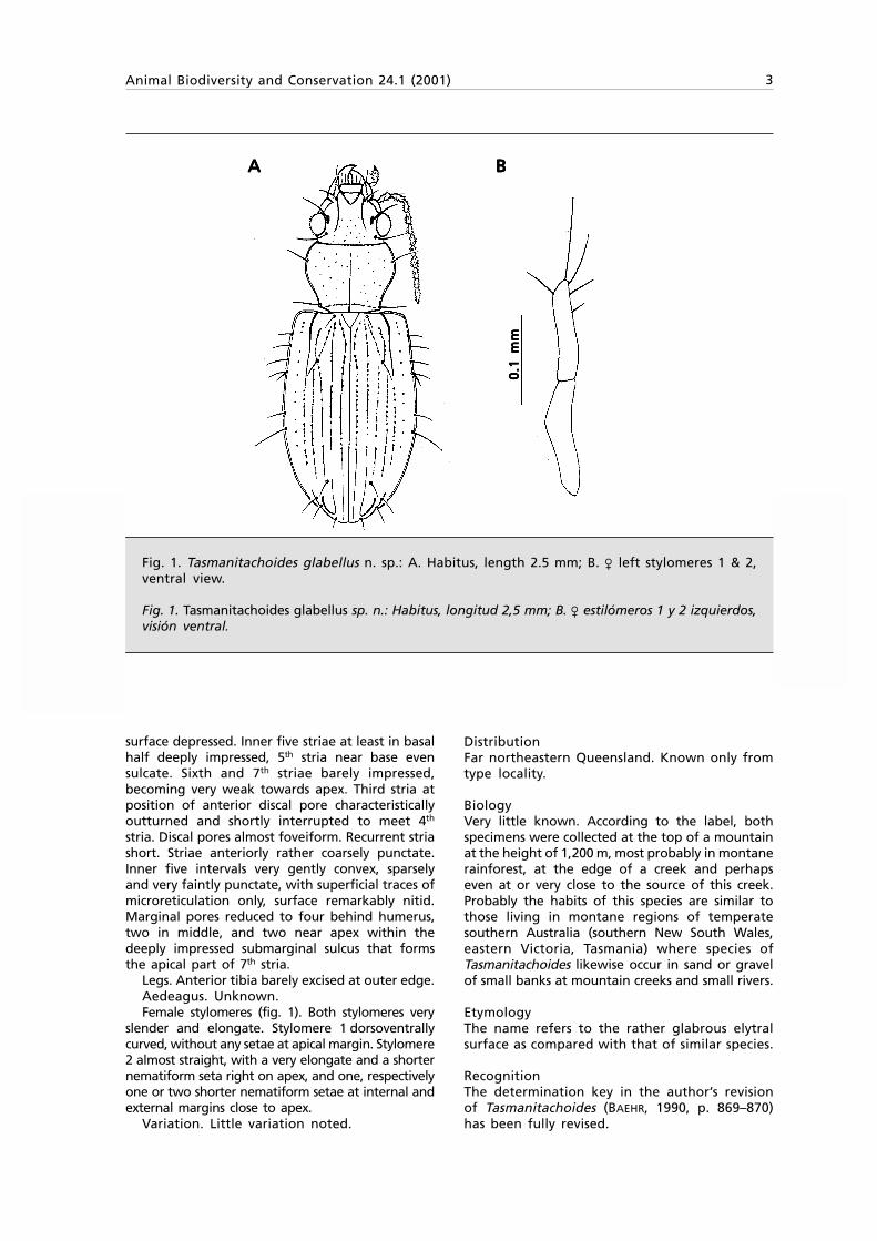
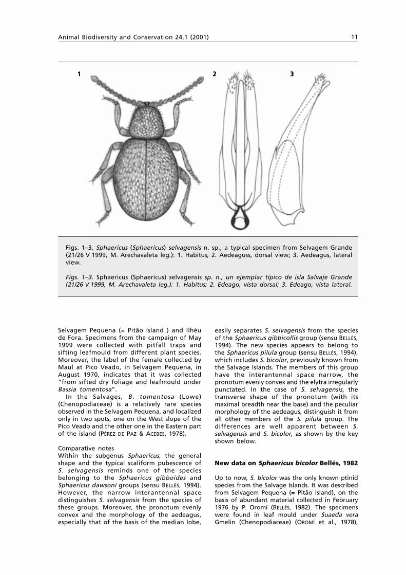
Fig. 1. Tasmanitachoides glabellus n. sp.: A. Habitus, length 2.5 mm; B. } left stylomeres 1 & 2,ventral view.
Fig. 1. Tasmanitachoides glabellus sp. n.: Habitus, longitud 2,5 mm; B. } estilómeros 1 y 2 izquierdos,visión ventral.
AAAAA B B B B B
0.1
mm
0.1
mm
0.1
mm
0.1
mm
0.1
mm
4 Baehr
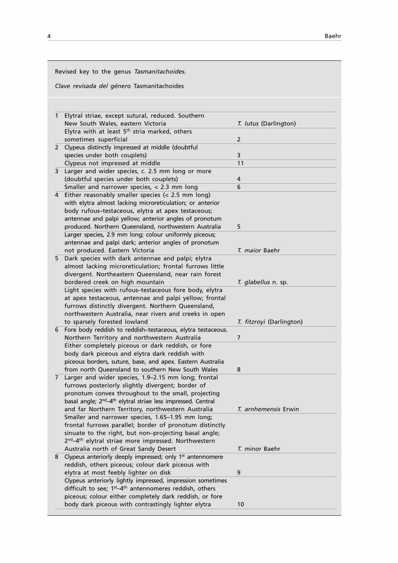
Revised key to the genus Tasmanitachoides.
Clave revisada del género Tasmanitachoides
1 Elytral striae, except sutural, reduced. SouthernNew South Wales, eastern Victoria T. lutus (Darlington)Elytra with at least 5th stria marked, otherssometimes superficial 2
2 Clypeus distinctly impressed at middle (doubtfulspecies under both couplets) 3Clypeus not impressed at middle 11
3 Larger and wider species, c. 2.5 mm long or more(doubtful species under both couplets) 4Smaller and narrower species, < 2.3 mm long 6
4 Either reasonably smaller species (< 2.5 mm long)with elytra almost lacking microreticulation; or anteriorbody rufous–testaceous, elytra at apex testaceous;antennae and palpi yellow; anterior angles of pronotumproduced. Northern Queensland, northwestern Australia 5Larger species, 2.9 mm long; colour uniformly piceous;antennae and palpi dark; anterior angles of pronotumnot produced. Eastern Victoria T. maior Baehr
5 Dark species with dark antennae and palpi; elytraalmost lacking microreticulation; frontal furrows littledivergent. Northeastern Queensland, near rain forestbordered creek on high mountain T. glabellus n. sp.Light species with rufous–testaceous fore body, elytraat apex testaceous, antennae and palpi yellow; frontalfurrows distinctly divergent. Northern Queensland,northwestern Australia, near rivers and creeks in opento sparsely forested lowland T. fitzroyi (Darlington)
6 Fore body reddish to reddish–testaceous, elytra testaceous.Northern Territory and northwestern Australia 7Either completely piceous or dark reddish, or forebody dark piceous and elytra dark reddish withpiceous borders, suture, base, and apex. Eastern Australiafrom north Queensland to southern New South Wales 8
7 Larger and wider species, 1.9–2.15 mm long; frontalfurrows posteriorly slightly divergent; border ofpronotum convex throughout to the small, projectingbasal angle; 2nd–4th elytral striae less impressed. Centraland far Northern Territory, northwestern Australia T. arnhemensis ErwinSmaller and narrower species, 1.65–1.95 mm long;frontal furrows parallel; border of pronotum distinctlysinuate to the right, but non–projecting basal angle;2nd–4th elytral striae more impressed. NorthwesternAustralia north of Great Sandy Desert T. minor Baehr
8 Clypeus anteriorly deeply impressed; only 1st antennomerereddish, others piceous; colour dark piceous withelytra at most feebly lighter on disk 9Clypeus anteriorly lightly impressed, impression sometimesdifficult to see; 1st–4th antennomeres reddish, otherspiceous; colour either completely dark reddish, or forebody dark piceous with contrastingly lighter elytra 10
Animal Biodiversity and Conservation 24.1 (2001) 5
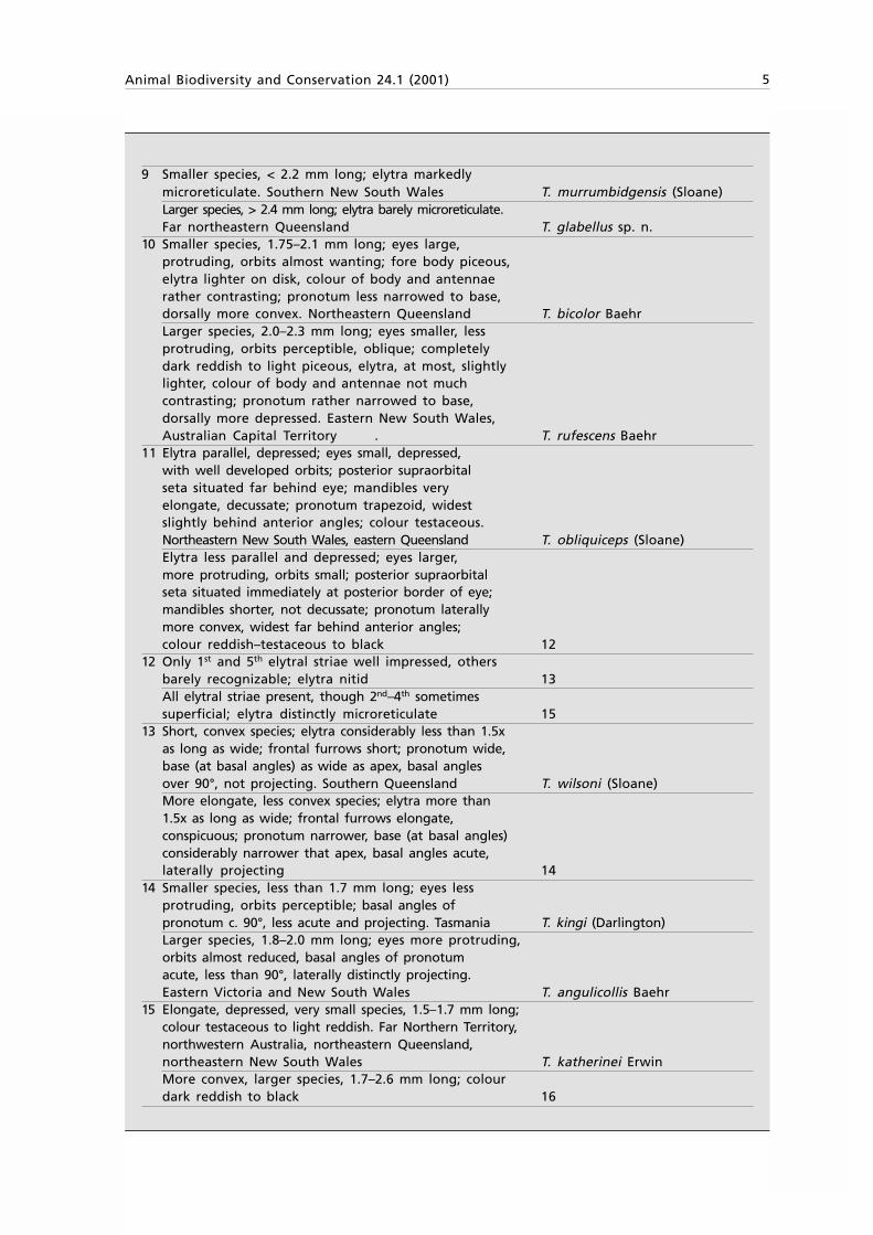
9 Smaller species, < 2.2 mm long; elytra markedlymicroreticulate. Southern New South Wales T. murrumbidgensis (Sloane)Larger species, > 2.4 mm long; elytra barely microreticulate.Far northeastern Queensland T. glabellus sp. n.
10 Smaller species, 1.75–2.1 mm long; eyes large,protruding, orbits almost wanting; fore body piceous,elytra lighter on disk, colour of body and antennaerather contrasting; pronotum less narrowed to base,dorsally more convex. Northeastern Queensland T. bicolor BaehrLarger species, 2.0–2.3 mm long; eyes smaller, lessprotruding, orbits perceptible, oblique; completelydark reddish to light piceous, elytra, at most, slightlylighter, colour of body and antennae not muchcontrasting; pronotum rather narrowed to base,dorsally more depressed. Eastern New South Wales,Australian Capital Territory . T. rufescens Baehr
11 Elytra parallel, depressed; eyes small, depressed,with well developed orbits; posterior supraorbitalseta situated far behind eye; mandibles veryelongate, decussate; pronotum trapezoid, widestslightly behind anterior angles; colour testaceous.Northeastern New South Wales, eastern Queensland T. obliquiceps (Sloane)Elytra less parallel and depressed; eyes larger,more protruding, orbits small; posterior supraorbitalseta situated immediately at posterior border of eye;mandibles shorter, not decussate; pronotum laterallymore convex, widest far behind anterior angles;colour reddish–testaceous to black 12
12 Only 1st and 5th elytral striae well impressed, othersbarely recognizable; elytra nitid 13All elytral striae present, though 2nd–4th sometimessuperficial; elytra distinctly microreticulate 15
13 Short, convex species; elytra considerably less than 1.5xas long as wide; frontal furrows short; pronotum wide,base (at basal angles) as wide as apex, basal anglesover 90°, not projecting. Southern Queensland T. wilsoni (Sloane)More elongate, less convex species; elytra more than1.5x as long as wide; frontal furrows elongate,conspicuous; pronotum narrower, base (at basal angles)considerably narrower that apex, basal angles acute,laterally projecting 14
14 Smaller species, less than 1.7 mm long; eyes lessprotruding, orbits perceptible; basal angles ofpronotum c. 90°, less acute and projecting. Tasmania T. kingi (Darlington)Larger species, 1.8–2.0 mm long; eyes more protruding,orbits almost reduced, basal angles of pronotumacute, less than 90°, laterally distinctly projecting.Eastern Victoria and New South Wales T. angulicollis Baehr
15 Elongate, depressed, very small species, 1.5–1.7 mm long;colour testaceous to light reddish. Far Northern Territory,northwestern Australia, northeastern Queensland,northeastern New South Wales T. katherinei ErwinMore convex, larger species, 1.7–2.6 mm long; colourdark reddish to black 16

6 Baehr
16 On the average smaller species, 1.7–2.3 mm long,rather depressed; clypeus faintly impressed; coloureither rather uniformly dark reddish, or piceouswith disk of each elytron contrastingly lighter 17On the average larger species, 2.1–2.6 mm long,more convex; clypeus not at all impressed; colouruniformly dark piceous to black, or piceous withelytra slightly (not contrastingly) lighter 18
17 Smaller species, 1.75–2.1 mm long; eyes large,protruding, orbits almost wanting; fore body piceous;elytra lighter on disk, colour of body and antennaerather contrasting; pronotum less narrowed to base,dorsally more convex. Northeastern Queensland T. bicolor BaehrLarger species, 2.0–2.3 mm long; eyes smaller, lessprotruding, orbits perceptible, oblique; completelydark reddish to light piceous, elytra, at most, slightlylighter, colour of body and antennae not muchcontrasting; pronotum rather narrowed to base,dorsally more depressed. Eastern New South Wales,Australian Capital Territory T. rufescens Baehr
18 Elytral striae, including 5th, strongly impressed 19Elytral striae, especially 5th, rather superficial.Eastern Victoria, southern New South Wales T. wattsense (Blackburn)
19 Colour uniformly dark piceous to almost black;antennae completely dark. Tasmania T. hobarti (Blackburn)Colour piceous, disk of elytra slightly lighter;basal antennomeres reddish. Northeastern NewSouth Wales T. leai (Sloane)
RemarksWith respect to the distinctly impressed clypeus, T.glabellus clearly belongs to the T. murrumbidgensis–group within the genus Tasmanitachoides. Thecombination of its dark colour and almost glabroussurface, however, at once distinguishes this speciesfrom all known species. Moreover, the dark colouris also unique within all Tasmanitachoides knownso far to occur in northern tropical Australia. Allthose species are either completely reddish ortestaceous (arnhemensis, fitzroyi, katherinei, minor,obliquiceps), or are at least bicolourous with darkfore–body though lighter elytra (bicolor). In contrast,almost all of the southern species are completelydark.
According to ERWIN’s (1972), DARLINGTON’s (1962:“gravel by brooks”), and the authors observations,in temperate Australia Tasmanitachoides arecommonly found at small rivers and mountainbrooks, even in shaded places, and commonly alsoat high altitudes. The species living in tropicalAustralia, however, are generally found in gravelsand sands of lakes, rivers and creeks of openlowlands, commonly even in comparatively arid
regions. Here, while exposed to the bright sun,their reddish or testaceous colour corresponds wellwith the colour of the substratum they live on andin —namely light coloured, at most light reddish—gravels and sands.
It has been postulated that the habits near streamsin temperate montane regions is regarded theoriginal mode of life for the genus Tasmanitachoides,whereas their occurrence in the tropical regions ofnorthern Australia is secondary (BAEHR, 1990). If thisassumption is true, then the occurrence of a darkcoloured species living at shaded rainforest creeksin montane northern Queensland would be quitesurprising, because this would mean a relictoccurrence with an ancient mode of life far northof the roots of this ancient genus that most probablyoriginated somewhere in temperate southeasternAustralia.
This assumption seems rather unlikely at firstglance, though within recent years a number ofexamples of definitely southern groups weredetected that have members far north in thetropics and subtropics well outside of theirrecognized range. Carabid examples for this
Animal Biodiversity and Conservation 24.1 (2001) 7
distribution pattern are two merizodine species ofthe genus Sloaneana Csiki which occur onLamington Plateau of south–eastern Queensland(BAEHR, in press), or the occurrence and remakabletaxonomic radiation of the psydrine generaRaphetis Moore, Sitaphe Moore, and of amblytelinePsydrinae in the wet tropics of North Queensland(unpublished records), or even the discovery of apeculiar (yet undescribed) new genus of thedefinitely “antarctic” subfamily Migadopinae,likewise in tropical North Queensland.
It follows from these examples, which couldbe complemented by certain non–carabidexamples, that remnants of the southerntemperate “Antarctic” faunal element ofAustralia are still present even in tropicalnorthern Queensland, and furthermore that thisdistribution pattern is probably more commonthan was believed to date. If related to thegeographic history of Australia, these examplesdemonstrate that various elements of thesouthern fauna were somehow trapped onmountains and tablelands of eastern and north–eastern Queensland during Australia’s drift tothe north during the Tertiary period. As a result,they can now be found high up in environmentswhich —although allowing them to survivethere— prevent their contact with their southerncounterparts and also prevent any furtherspreading.
When seen in the light of the biogeographicalhistory of north–eastern Australia, the unexpecteddiscovery of the new Tasmanitachoides addsvaluable information towards understanding thecomplexity of the montane fauna of the wettropics of northern Queensland.
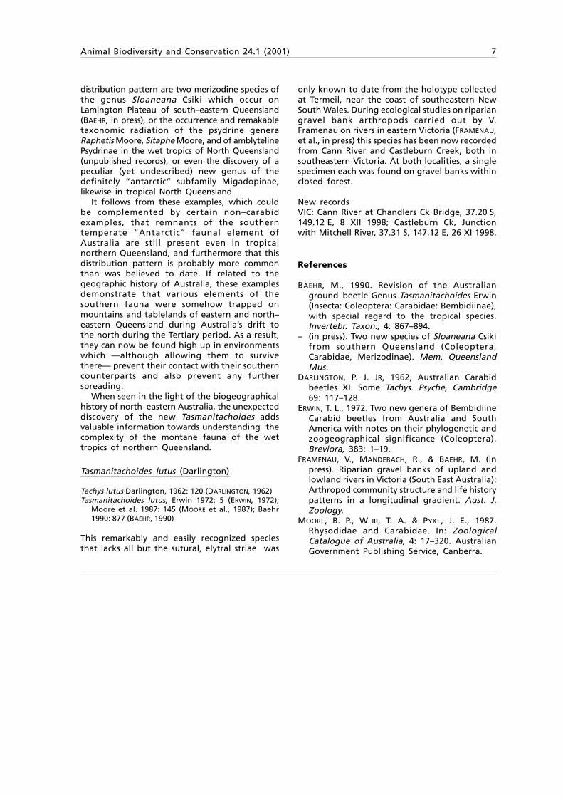
Tasmanitachoides lutus (Darlington)
Tachys lutus Darlington, 1962: 120 (DARLINGTON, 1962)Tasmanitachoides lutus, Erwin 1972: 5 (ERWIN, 1972);
Moore et al. 1987: 145 (MOORE et al., 1987); Baehr1990: 877 (BAEHR, 1990)
This remarkably and easily recognized speciesthat lacks all but the sutural, elytral striae was
only known to date from the holotype collectedat Termeil, near the coast of southeastern NewSouth Wales. During ecological studies on ripariangravel bank arthropods carried out by V.Framenau on rivers in eastern Victoria (FRAMENAU,et al., in press) this species has been now recordedfrom Cann River and Castleburn Creek, both insoutheastern Victoria. At both localities, a singlespecimen each was found on gravel banks withinclosed forest.
New recordsVIC: Cann River at Chandlers Ck Bridge, 37.20 S,149.12 E, 8 XII 1998; Castleburn Ck, Junctionwith Mitchell River, 37.31 S, 147.12 E, 26 XI 1998.
References
BAEHR, M., 1990. Revision of the Australianground–beetle Genus Tasmanitachoides Erwin(Insecta: Coleoptera: Carabidae: Bembidiinae),with special regard to the tropical species.Invertebr. Taxon., 4: 867–894.
– (in press). Two new species of Sloaneana Csikifrom southern Queensland (Coleoptera,Carabidae, Merizodinae). Mem. QueenslandMus.
DARLINGTON, P. J. JR, 1962, Australian Carabidbeetles XI. Some Tachys. Psyche, Cambridge69: 117–128.
ERWIN, T. L., 1972. Two new genera of BembidiineCarabid beetles from Australia and SouthAmerica with notes on their phylogenetic andzoogeographical significance (Coleoptera).Breviora, 383: 1–19.
FRAMENAU, V., MANDEBACH, R., & BAEHR, M. (inpress). Riparian gravel banks of upland andlowland rivers in Victoria (South East Australia):Arthropod community structure and life historypatterns in a longitudinal gradient. Aust. J.Zoology.
MOORE, B. P., WEIR, T. A. & PYKE, J. E., 1987.Rhysodidae and Carabidae. In: ZoologicalCatalogue of Australia, 4: 17–320. AustralianGovernment Publishing Service, Canberra.

9Animal Biodiversity and Conservation 24.1 (2001)
© 2001 Museu de ZoologiaISSN: 1578–665X
Bellés, X., 2001. Description of Sphaericus selvagensis n. sp. from the Salvage Islands, and new data onSphaericus bicolor Bellés (Coleoptera, Ptinidae). Animal Biodiversity and Conservation, 24.1: 9–13.
AbstractAbstractAbstractAbstractAbstractDescription of Sphaericus selvagensis n. sp. from the Salvage Islands, and new data on Sphaericus bicolor Bellés(Coleoptera, Ptinidae).— Sphaericus (Sphaericus) selvagensis n. sp. is described from the Salvage islands. WithSphaericus (Sphaericus) bicolor Bellés, this new species is only the second ptinid beetle reported from theseislands. S. selvagensis belongs to the Sphaericus pilula group, which also includes S. bicolor. However, thetransverse shape of the pronotum (with its maximal breadth near the base) and the peculiar morphology of theaedeagus, distinguish S. selvagensis from all other members of the S. pilula group. S. selvagensis lives in all themajor islands of the Selvagens archipelago: Selvagem Grande, Selvagem Pequena and Ilhéu de Fora.
Key words: Coleoptera, Ptinidae, Sphaericus, Salvage Islands.
ResumenResumenResumenResumenResumenDescripción de Sphaericus selvagensis sp. n. del archipiélago de las Salvajes, y nuevos datos sobre Sphaericusbicolor Bellés (Coleoptera, Ptinidae).— Se describe Sphaericus (Sphaericus) selvagensis sp. n. del archipiélago delas Salvajes. Junto a Sphaericus (Sphaericus) bicolor Bellés, esta nueva especie es el segundo coleóptero ptínidoregistrado en esas islas. S. selvagensis pertenece al grupo de Sphaericus pilula, que también incluye S. bicolor,aunque la forma transversa del pronoto (con anchura máxima cerca de la base) y la peculiar morfología deledeago distinguen a S. selvagensis de los restantes miembros de grupo de S. pilula. S. selvagensis vive en todaslas islas principales del archipiélago de las Salvajes: Salvaje Grande, Salvaje Pequeña (o Pitón Grande) y LaSalvajita (Ilhéu de Fora).
Palabras clave: Coleoptera, Ptinidae, Sphaericus, Islas Salvajes.
(Received: 1 X 01; Conditional acceptance: 10 X 01; Final acceptance: 20 X 01)
Xavier Bellés, Dept. of Physiology and Molecular Biodiversity, Inst. de Biologia Molecular de Barcelona (CID, CSIC),c/ Jordi Girona 18, 08034 Barcelona, Espanya (Spain).
e-mail: [email protected]
Description of Sphaericus selvagensis n. sp.from the Salvage Islands, and new data onSphaericus bicolor Bellés(Coleoptera, Ptinidae)
X. Bellés
10 Bellés
Introduction
The Salvage Islands lie in the Atlantic Oceanbetween the well–known archipelagos ofMadeira and Canaries (BRAVO & COELLO, 1978).Up to now, the only ptinid beetle reportedfrom the Selvagens is Sphaericus (Sphaericus)bicolor Bellés, described from Selvagem Pequena(= Pitão Island) (BELLÉS, 1982) and later recordedby ERBER & WHEATER (1987) from SelvagemGrande and Ilhéu de Fora. However, the studyof the ptinid beetles collected during a campaigncarried out in the Salvages in May 1999, in thecontext of the Project “Macaronesia 2000” ofthe Museo de Ciencias Naturales de Tenerife,has lead to the discovery of a new species ofSphaericus, which is described in the presentpaper. The data on the arthropods collectedduring this expedition of 1999 have beenreported by ARECHAVALETA et al. (2001).
The genus Sphaericus was proposed byWollaston as early as 1854, but has been thesubject of a relatively recent synopsis by BELLÉS
(1994), who divided it into three subgenera:Sphaericus, the members of which are charac-terized by having 11–segmented antennae,5–segmented male metatarsi, the base ofthe pronotum simple and the parameres ofthe aedeagus slender and pubescent only atthe apex; Nitpus Jacquelin du Val, whosetwo species have 9–segmented antennae and4–segmented male metatarsi; and DoramasusBellés, described in the same synopsis (BELLÉS,1994) as similar to Sphaericus s. str. but showingthe base of the pronotum protuberant and theparameres of the aedeagus robust and evenlypubescent.
With the exception of Sphaericus (Sphaericus)gibboides (Boieldieu), which is anthropophilousand nearly cosmopolitan (HINTON, 1941), andSphaericus (Sphaericus) niveus (Boieldieu),Sphaericus (Sphaericus) exiguus (Boieldieu) andSphaericus (Nitpus) ptinoides (Boieldieu), whichare known from sparse localities in theMediterranean area (BOIELDIEU, 1856; PIC, 1912;BELLÉS, 1994), all the other species of thesethree subgenera are endemic to islands ofAtlantic archipelagos.
The island groups include the Canaries(10 species), Madeira (nine species), Cape Verde(two species), Salvages (two species, includingthat described herein), and Açores (one species)(BELLÉS, 1994). More recently, the new subgenusLeasphaericus Bellés (1998) (BELLÉS, 1998) hasbeen proposed for two Australian species. Thesetaxa, in contrast with the Palaearctic Sphaericus,have a triangular scutellum easily visible fromabove.
Due to the morphology of the aedeagus andthe pronotum, the number of the segments inthe antennae and tarsi, and the hidden scutellum,the new species described below falls into thesubgenus Sphaericus Wollaston.
Description
Sphaericus (Sphaericus) selvagensis n. sp.
TypesHolotype: 1{ labelled “Islas Salvajes, SelvagemGrande, 21/26–V–1999, M. Arechavaleta leg.”(Museo de Ciencias Naturales, Santa Cruz deTenerife).
Paratypes: 84 specimens of both sexes with thesame label as the holotype; 6 specimens of bothsexes with the label “Islas Salvajes, SelvagemPequena, 25–V–1999, M. Arechavaleta leg.”; 1}labelled “Selvagem Pequena, Pico Veado, 21–8–70,Maul leg.”; 18 specimens of both sexes with thelabel “I. Selvagens, Pitão, 5–VI–1970, Maul leg.”; 1}labelled “Islas Salvajes, Ilhéu de Fora, 25–V–1999,M. Arechavaleta leg.” (Museo de Ciencias Naturales,Santa Cruz de Tenerife; Departamento de BiologíaAnimal, Universidad de La Laguna; Museo Nacionalde Ciencias Naturales, Madrid; Museu de Zoología,Barcelona; colls. Oromí, Bellés, Arechavaleta andGarcía Becerra).
Description of the male (fig. 1)Length: 1.2–1.8 mm (n = 12)
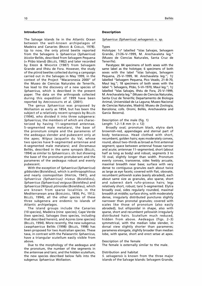
Broadly oval; pronotum black, elytra darkbrownish–red, appendages and sternal part ofbody testaceous. Head clothed with short,recumbent, golden hairs; eyes moderately convex,round, about two–thirds as broad as first antennalsegment; space between antennal fossae narrowand acute; antennae 11–segmented, short (abouthalf as long as body) and robust, segments 3 to10 oval, slightly longer than width. Pronotumevenly convex, transverse, sides feebly arcuate,maximal breadth near base; surface with verydense to contiguous granules each about twiceas large as eye facets; covered with flat, obovate,recumbent yellowish scales (easily abraded), eachabout same size as granules, also sparse, shortand suberect dark rufo–piceous hairs; legsrelatively short, robust; tarsi 5–segmented. Elytrabroadly oval, sides regularly rounded, maximalbreadth at middle; surface shiny, with moderatelydense, irregularly distributed punctures slightlynarrower than pronotal granules; covered withscales like those of pronotum (also easilyabraded), but ellipsoidal in shape, also withsparse, short and recumbent yellowish irregularlydistributed hairs. Scutellum much reduced,hidden from above. Aedeagus (figs. 2–3)symmetrical, with the median lobe slender, indorsal view slightly shorter than parameres;parameres elongate, slightly broader than medianlobe, with sparse, short and erect setae at apex.
Description of the femaleThe female is externally similar to the male.
Distribution and habitatS. selvagensis is known from the three majorislands of the Salvage Islands: Selvagem Grande,
Animal Biodiversity and Conservation 24.1 (2001) 11
Selvagem Pequena (= Pitão Island ) and Ilhéude Fora. Specimens from the campaign of May1999 were collected with pitfall traps andsifting leafmould from different plant species.Moreover, the label of the female collected byMaul at Pico Veado, in Selvagem Pequena, inAugust 1970, indicates that it was collected“from sifted dry foliage and leafmould underBassia tomentosa”.
In the Salvages, B. tomentosa (Lowe)(Chenopodiaceae) is a relatively rare speciesobserved in the Selvagem Pequena, and localizedonly in two spots, one on the West slope of thePico Veado and the other one in the Eastern partof the island (PÉREZ DE PAZ & ACEBES, 1978).
Comparative notesWithin the subgenus Sphaericus, the generalshape and the typical scaliform pubescence ofS. selvagensis reminds one of the speciesbelonging to the Sphaericus gibboides andSphaericus dawsoni groups (sensu BELLÉS, 1994).However, the narrow interantennal spacedistinguishes S. selvagensis from the species ofthese groups. Moreover, the pronotum evenlyconvex and the morphology of the aedeagus,especially that of the basis of the median lobe,
easily separates S. selvagensis from the speciesof the Sphaericus gibbicollis group (sensu BELLÉS,1994). The new species appears to belong tothe Sphaericus pilula group (sensu BELLÉS, 1994),which includes S. bicolor, previously known fromthe Salvage Islands. The members of this grouphave the interantennal space narrow, thepronotum evenly convex and the elytra irregularlypunctated. In the case of S. selvagensis, thetransverse shape of the pronotum (with itsmaximal breadth near the base) and the peculiarmorphology of the aedeagus, distinguish it fromall other members of the S. pilula group. Thedifferences are well apparent between S.selvagensis and S. bicolor, as shown by the keyshown below.
New data on Sphaericus bicolor Bellés, 1982
Up to now, S. bicolor was the only known ptinidspecies from the Salvage Islands. It was describedfrom Selvagem Pequena (= Pitão Island), on thebasis of abundant material collected in February1976 by P. Oromí (BELLÉS, 1982). The specimenswere found in leaf mould under Suaeda veraGmelin (Chenopodiaceae) (OROMÍ et al., 1978),
Figs. 1–3. Sphaericus (Sphaericus) selvagensis n. sp., a typical specimen from Selvagem Grande(21/26 V 1999, M. Arechavaleta leg.): 1. Habitus; 2. Aedeaguss, dorsal view; 3. Aedeagus, lateralview.
Figs. 1–3. Sphaericus (Sphaericus) selvagensis sp. n., un ejemplar típico de isla Salvaje Grande(21/26 V 1999, M. Arechavaleta leg.): 1. Habitus; 2. Edeago, vista dorsal; 3. Edeago, vista lateral.
11111 22222 33333
12 Bellés
which is one of the most abundant and typicalplants of the Salvages, either in the SelvagemGrande or in the Selvagem Pequena (PÉREZ DE PAZ
& ACEBES, 1978). Interestingly, no specimens of S.selvagensis were collected during this 1976campaign. Almost simultaneously, SERRANO (1983)recorded an undetermined species of Sphaericusfrom the Selvagem Grande (1 specimen) andSelvagem Pequena (549 specimens). Seventy–twospecimens were examined by the author fromthis large series and all were S. bicolor. Thespecimen from Selvagem Grande was collectedon S. vera and those from Selvagem Pequena onElytrigia junceiforme A. et D. Löve (Poaceae)(SERRANO, 1983). A. junceiforme is relatively rarein Selvagem Pequena, being found in a singlelocality on the Eastern part of the island. Morerecently, ERBER & WHEATER (1987) have reportedthe identification of 89 specimens of S. bicolorfrom Selvagem Pequena, 4 from Ilhéu de Foraand 1 from Selvagem Grande, which had beencollected by Backhuys in 1968 and deposited inthe Museum of Funchal. Materials from theexpedition in 1999 studied in the present workincluded specimens of S. bicolor mixed with thenew S. selvagensis, and was collected using pitfalltraps and sifting leaf mould from different plants.The number of specimens of both species presentin these and in other samples studied by theauthor is indicated in table 1. These data suggestthat any of the two species may be very abundant
Key to the Sphaericus of the Salvage Islands.
Clave para los Sphaericus de las Islas Salvajes.
1 Antennae long and slender, clearly longer thanhalf the body, with the segments 2–10 subcylindrical,nearly longer than width. Pronotum longer thanwidth, with the maximal breadth near the middle.Legs long and slender. Elytra ellipsoidal (fig. 1from BELLÉS, 1982). Aedeagus in dorsal view withthe median lobe much shorter than the parameres;parameres clearly broader than the median lobe(figs. 3–4 from BELLÉS, 1982) S. bicolor Bellés, 1982Antennae short and robust, about half as long asthe body, with the segments 2–10 oval, slightly longerthan width. Pronotum transverse, with the maximalbreadth near the base. Legs short and robust.Elytra broadly oval (fig. 1, present paper).Aedeagus in dorsal view with the median lobealmost as long as the parameres; parameresslightly broader than the median lobe(figs. 2–3, present paper) S. selvagensis n. sp.
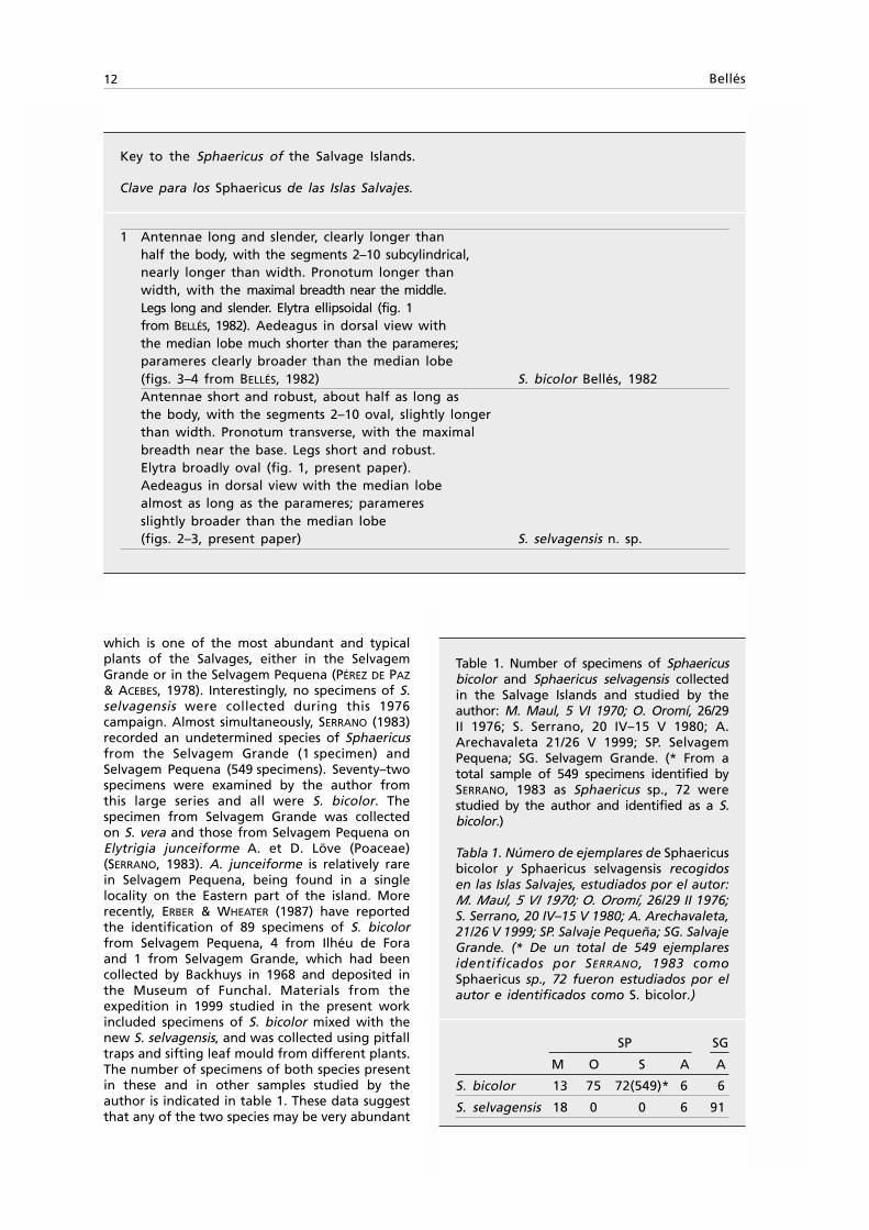
Table 1. Number of specimens of Sphaericusbicolor and Sphaericus selvagensis collectedin the Salvage Islands and studied by theauthor: M. Maul, 5 VI 1970; O. Oromí, 26/29II 1976; S. Serrano, 20 IV–15 V 1980; A.Arechavaleta 21/26 V 1999; SP. SelvagemPequena; SG. Selvagem Grande. (* From atotal sample of 549 specimens identified bySERRANO, 1983 as Sphaericus sp., 72 werestudied by the author and identified as a S.bicolor.)
Tabla 1. Número de ejemplares de Sphaericusbicolor y Sphaericus selvagensis recogidosen las Islas Salvajes, estudiados por el autor:M. Maul, 5 VI 1970; O. Oromí, 26/29 II 1976;S. Serrano, 20 IV–15 V 1980; A. Arechavaleta,21/26 V 1999; SP. Salvaje Pequeña; SG. SalvajeGrande. (* De un total de 549 ejemplaresidentificados por SERRANO, 1983 comoSphaericus sp., 72 fueron estudiados por elautor e identificados como S. bicolor.)
SP SG
M O S A A
S. bicolor 13 75 72(549)* 6 6
S. selvagensis 18 0 0 6 91
Animal Biodiversity and Conservation 24.1 (2001) 13
depending on the time and eventually on theprecise site of collection. All data (BELLÉS, 1982;ERBER & WHEATER, 1987; present results) indicatethat both S. bicolor and S. selvagensis arewidespread in the three main islands of thearchipelago: Selvagem Grande, SelvagemPequena (= Pitão Island) and Ilhéu de Fora.
Acknowledgements
Thanks are due to Pedro Oromí for critical readingof the manuscript and for sending abundantmaterial of Sphaericus from the Salvages,especially those collected by M. Arechavaletaduring the expedition of May 1999, in the contextof the Project “Macaronesia 2000” of the Museode Ciencias Naturales de Tenerife. Keith Philipsalso reviewed the manuscript. Artur R. M. Serranosent a large sample of S. bicolor from SelvagemPequena collected during the ExpediçãoZoológica aos Arquipélagos da Madeira e dasSelvagens (30 de Abril–15 de Maio, 1980).
References
ARECHAVALETA, M., ZURITA, N. & OROMÍ, P., 2001.Nuevos datos sobre la fauna de artrópodos delas Islas Salvajes. Rev. Acad. Canar. Cienc., 12(3–4): 83–99 (2000).
BELLÉS, X., 1982. El primer representante de lafamilia Ptinidae (Col.) de las Islas Salvajes:Sphaericus bicolor n. sp. Vieraea, 11: 103–108.
– 1994. El género Sphaericus Wollaston, 1854(Coleoptera: Ptinidae). Boln. Asoc. esp. Ent.,18: 61–79.
– 1998. A new subgenus and two new species ofSphaericus Wollaston (Coloptera, Ptinidae)from western Australia. Eur. J. Entomol., 95:263–268.
BOIELDIEU, A., 1856. Monographie des Ptiniores. Annls.Soc. ent. Fr., (3)4: 285–315, 487–504, 629–686.
BRAVO, T. & COELLO, J., 1978. Descripcióngeográfica del Archipiélago de las Salvajes. In:Contribución al estudio de la historia naturalde las Islas Salvajes: 9–14. Aula de Cultura deTenerife, Santa Cruz de Tenerife.
ERBER, D. & WHEATER, C. F., 1987. The Coleopteraof the Selvagem Islands, including a catalogueof the pecimens in the Museu Municipal doFunchal. Bol. Mus. Mun. Funchal, 39(193):156–187.
HINTON, H. E., 1941. The Ptinidae of economicimportance. Bull. ent. Res., 31: 331–381.
OROMÍ, P., BAEZ, M. & MACHADO, A., 1978.Contribución al estudio de los artrópodos de lasIslas Salvajes. In: Contribución al estudio de lahistoria natural de las Islas Salvajes: 178–194.Aula de Cultura de Tenerife, Santa Cruz deTenerife.
PÉREZ DE PAZ, P. L. & ACEBES, J. R., 1978. Las IslasSalvajes: Contribución al conocimiento de suflora y vegetación. In: Contribución al estudiode la historia natural de las Islas Salvajes: 79–104. Aula de Cultura de Tenerife, Santa Cruz deTenerife.
PIC, M., 1912. Ptinidae. In: ColeopterorumCatalogus, 41: 1–46 (W. Junk & S. Schenkling,Eds.). W. Junk, Berlin.
SERRANO, A. R. M., 1983. Os coleopteros doArquipélago das Selvagens. In: Act. I Congr. IbéricoEnt., 2: 759–776. Servicio de Publicaciones de laUniversidad de León, León.

15Animal Biodiversity and Conservation 24.1 (2001)
© 2001 Museu de ZoologiaISSN: 1578–665X
Survival of a small translocatedProcolobus kirkii population onPemba Island
A. Camperio Ciani, L. Palentini & E. Finotto
Camperio Ciani, A., Palentini, L. & Finotto, E., 2001. Survival of a small translocated Procolobus kirkii populationon Pemba Island. Animal Biodiversity and Conservation, 24.1: 15–18 .
AbstractAbstractAbstractAbstractAbstractSurvival of a small translocated Procolobus kirkii population on Pemba Island.— A survey to evaluate thedistribution of Procolobus kirkii on Pemba island (Tanzania) was conducted, 20 years after they had beentranslocated from Zanzibar in the Ngezi forest park. A team of both expert and trained observers, guided bythe authors, censused 68.3 linear km of forest, corresponding to an estimated area of 3.5 km2 (63.6%) of theprotected Ngezi forested area of 5.5 km2. Nineteen groups of Cercopithecus aethiops were observed, with atotal of 166 animals and an estimated density of 47.43 individuals per km2, and only one troop of Procolobuskirkii. Supplemented by interviewing the local people we obtained an estimate of 15–30 P. kirkii, including asmall troop outside the protected area. This small population survived but did not increase, possibly due toadverse relations with humans.
Key word: Procolobus kirkii, Translocated population, Density, Conservation, Pemba Island.
ResumenResumenResumenResumenResumenSupervivencia de una pequeña población trasladada de Procolobus kirkii en la isla de Pemba.— Se realizó unestudio para evaluar la distribución de Procolobus kirkii en la isla de Pemba (Tanzania), veinte años después deque fuera trasladada desde Zanzíbar al Parque Ngezi. Un equipo de observadores expertos y entrenados,guiados por los autores, efectuó un censo a lo largo de 68,3 km lineales de bosque, correspondiente a un áreaestimada de 3,5 km2 (63,6%) del área protegida del bosque de Ngezi de 5,5 km2. Se observaron 19 grupos deCercopithecus aethiops, con un total de 166 animales y una densidad estimada de 47,43 individuos/km2, y sóloun grupo de Procolobus kirkii. Complementando los datos con entrevistas a la población local se obtuvo unaestimación de 15–30 ejemplares de P. kirkii, incluyendo un pequeño grupo localizado fuera del área protegida.Este pequeño grupo sobrevivía pero no se incrementaba en número, posiblemente debido a las relacionesadversas con los humanos.
Palabras clave: Procolobus kirkii, Población trasladada, Densidad, Conservación, Isla de Pemba.
(Received: 23 VII 01; Final acceptance: 2 X 01)
Andrea Camperio Ciani(1), Loris Palentini & Enrica Finotto, Dip. di Psicologia Generale, Universita’degli Studi diPadova, 8 via Venezia, 35139 Padova, Italy.
(1)e-mail: [email protected]
16 Camperio Ciani et al.
Introduction
Procolobus kirkii, member of the Colobinae family,represents one of Africa’s most endangeredprimate species.
It is mainly an arboreal and folivorous species,sympatric but not in competition with Cercopitecusaethiops which is mainly frugivorous (SIEX &STRUHSAKER, 1999a). It has been reported that tocontrast the toxins contained in certain fruit P.kirkii eats a small quantity of charcoal which allowa slower, but otherwise impossible, digestion(STRUHSAKER et al., 1997). Its ideal habitats inZanzibar are areas with ground water, swampforest, scrub forest or mangrove swamp.
Troops are numerous and can include morethan 80 individuals. They have a multi–malestructure which is unusual for the Colobinaefamily, with a 1:2 sex ratio with adult females.Fecundity is about 1.5 new–born every 2 yearsand infant care is intense and shared by severalrelated females. Infanticide is common as inmost Colobinae when a new male joins thegroup.
P. kirkii is endemic and confined to the islandof Zanzibar. It is present in 3 different forestswith a total population of about 1,500 individuals(Zanzibar Unpublished Government Census,1981). Two decades ago specimens were movedto new areas, mostly small islands, in order totry to inhibit their decline leading to a rapidextinction. These animals are threatened bymassive deforestation and furthermore arehunted for their meat and for pet markets(STRUHSAKER & SIEX, 1996).
An assessment of the present survival rate andthe diffusion of the small Procolobus population(14 individuals) translocated from Jozani Park andintroduced in the region of Ngezi Forest, in 1974(STRUHSAKER & SIEX, 1998) in the north of PembaIsland is reported in this study.
Methods
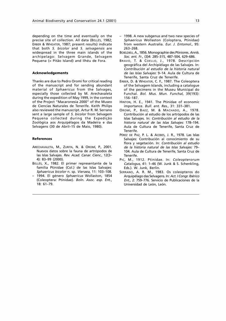
Data were collected from 15th–20th October2000. To census the region as thoroughly aspossible the forest was divided into 14 transects(fig. 1) varying in length from about 2 to 8 km(totally 68.3 km). Each transect segment wasidentified by a 1:50,000 topographical map, andlocated in the field with a GPS and compass.
Teams included volunteers who underwentprior training in the Jozani Forest of Zanzibar toidentify the different species of monkeys untilconsensus with the trainers reached completeagreement.
Transects were walked with a fixed departure,arrival and direction. Each transect was walkedby a rotating team of 3 to 4 people, scaled inexperience in the field, and randomly changedeach day in order to avoid individual bias in datacollection (CAMPERIO CIANI et al., 2001).
Forest quality was classified into five mainhabitat types: gallery forest, mangrove, savannah,swamp and cultivations. To estimate the densityof monkeys in each different habitat wecalculated the width of our transects in eachhabitat. To assess the width, as for the case oftransects of indefinite width (CAUGHLEY, 1977),we used the average distance at first sighting ofthe Cercopithecus aethiops in that habitat.
Field survey was supplemented with interviewsamong the local people living in villages aroundand within the Ngezi Forest in search of witnessesand information about the presence of P. kirkii.
Results and discussion
A distance of approximately 68.3 km was walkedin the five various habitats inside the park.Considering the length and the relative width ofour transects, during the study about 3.5 km2,63.6% of the total forested area of the park wasmonitored (5.5 km2) (table 1).
Sightings almost exclusively regard C. aethiops.A total of 19 troops were located from amongall habitats except swamps. A total of 166 animalswere observed inside the forested region(table 1), mainly sighted in the gallery forest.The estimated total density of C. aethiops in thepark area is 47.43 individuals per km2.
Only an elusive sighting of P. kirkii was noted,this occurring in the gallery forest in the south
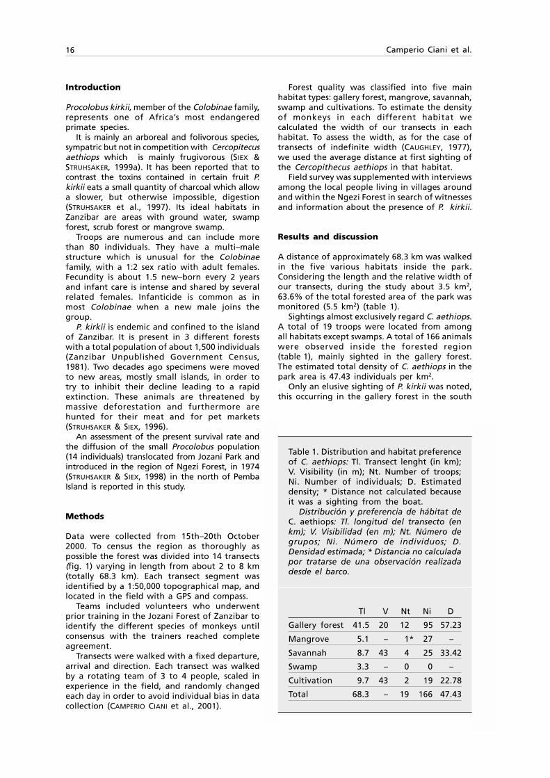
Table 1. Distribution and habitat preferenceof C. aethiops: Tl. Transect lenght (in km);V. Visibility (in m); Nt. Number of troops;Ni. Number of individuals; D. Estimateddensity; * Distance not calculated becauseit was a sighting from the boat.
Distribución y preferencia de hábitat deC. aethiops: Tl. longitud del transecto (enkm); V. Visibilidad (en m); Nt. Número degrupos; Ni. Número de individuos; D.Densidad estimada; * Distancia no calculadapor tratarse de una observación realizadadesde el barco.
Tl V Nt Ni D
Gallery forest 41.5 20 12 95 57.23
Mangrove 5.1 – 1* 27 –
Savannah 8.7 43 4 25 33.42
Swamp 3.3 – 0 0 –
Cultivation 9.7 43 2 19 22.78
Total 68.3 – 19 166 47.43
Animal Biodiversity and Conservation 24.1 (2001) 17
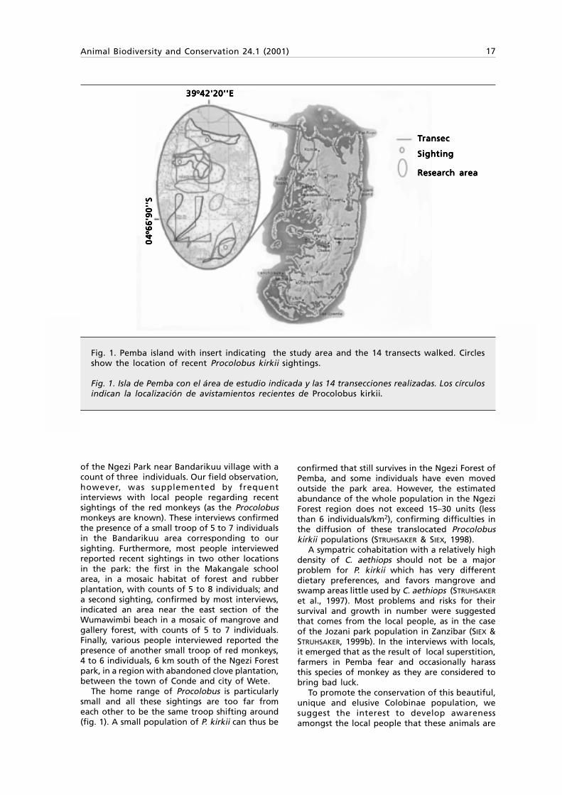
Fig. 1. Pemba island with insert indicating the study area and the 14 transects walked. Circlesshow the location of recent Procolobus kirkii sightings.
Fig. 1. Isla de Pemba con el área de estudio indicada y las 14 transecciones realizadas. Los círculosindican la localización de avistamientos recientes de Procolobus kirkii.
of the Ngezi Park near Bandarikuu village with acount of three individuals. Our field observation,however, was supplemented by frequentinterviews with local people regarding recentsightings of the red monkeys (as the Procolobusmonkeys are known). These interviews confirmedthe presence of a small troop of 5 to 7 individualsin the Bandarikuu area corresponding to oursighting. Furthermore, most people interviewedreported recent sightings in two other locationsin the park: the first in the Makangale schoolarea, in a mosaic habitat of forest and rubberplantation, with counts of 5 to 8 individuals; anda second sighting, confirmed by most interviews,indicated an area near the east section of theWumawimbi beach in a mosaic of mangrove andgallery forest, with counts of 5 to 7 individuals.Finally, various people interviewed reported thepresence of another small troop of red monkeys,4 to 6 individuals, 6 km south of the Ngezi Forestpark, in a region with abandoned clove plantation,between the town of Conde and city of Wete.
The home range of Procolobus is particularlysmall and all these sightings are too far fromeach other to be the same troop shifting around(fig. 1). A small population of P. kirkii can thus be
confirmed that still survives in the Ngezi Forest ofPemba, and some individuals have even movedoutside the park area. However, the estimatedabundance of the whole population in the NgeziForest region does not exceed 15–30 units (lessthan 6 individuals/km2), confirming difficulties inthe diffusion of these translocated Procolobuskirkii populations (STRUHSAKER & SIEX, 1998).
A sympatric cohabitation with a relatively highdensity of C. aethiops should not be a majorproblem for P. kirkii which has very differentdietary preferences, and favors mangrove andswamp areas little used by C. aethiops (STRUHSAKER
et al., 1997). Most problems and risks for theirsurvival and growth in number were suggestedthat comes from the local people, as in the caseof the Jozani park population in Zanzibar (SIEX &STRUHSAKER, 1999b). In the interviews with locals,it emerged that as the result of local superstition,farmers in Pemba fear and occasionally harassthis species of monkey as they are considered tobring bad luck.
To promote the conservation of this beautiful,unique and elusive Colobinae population, wesuggest the interest to develop awarenessamongst the local people that these animals are
3939393939ooooo42'20''E42'20''E42'20''E42'20''E42'20''E
04
04
04
04
04
oooo o6
6'9
0''
S6
6'9
0''
S6
6'9
0''
S6
6'9
0''
S6
6'9
0''
STTTTTransecransecransecransecransec
SightingSightingSightingSightingSighting
Research areaResearch areaResearch areaResearch areaResearch area

18 Camperio Ciani et al.
not only harmless but that their protection andan increase in numbers will eventually bebeneficial in attracting tourists to the NgeziPark, as occurred in Zanzibar.
Acknowledgements
We wish to thank K. Siex for suggesting thisstudy and introducing us to the Jozani Park. Wethank the direction of the Ngezi Forest Park fortheir enthusiastic collaboration in the field.Special thanks to all the members of the GEAPemba expedition who funded and volunteeredin this project.
References
CAMPERIO CIANI, A., MARTINOLI, L., CAPILUPPI, C.,ARAHOU, M. & MOUNA, M., 2001. Effect ofWater Availability and Habitat Quality on Bark-Stripping in Barbary Macaques. ConservationBiology, 15(1): 259–265.
CAUGLEY, G., 1977. Analysis of vertebratepopulations. John Wiley and Sons Ltd., NY.
COONEY, D. O. & STRUHSAKER, T. T., 1997. Adsorptivecapacity of charcoal eaten by Zanzibar redcolobus monkeys: implications for reducingdietary toxins. International Journal ofPrymatology, 18(2): 235–246.
SIEX, K. S. & STRUHSAKER, T. T., 1999a. Colobusmonkeys and coconuts: A study of perceivedhuman–wildlife conflicts. Journal of AppliedEcology, 36(6): 1,009–1,020.
– 1999b. Ecology of the Zanzibar red colobusmonkey: demographic variability and habitatstability. International Journal of Prymatology,20(2): 163–192.
STRUHSAKER, T. T., COONEY, D. O. & SIEX, K. S., 1997.Charcoal consumption by Zanzibar red colobusmonkey: its function and its ecological anddemographic consequences. InternationalJournal of Prymatology, 18(1): 61–72.
STRUHSAKER, T. T. & SIEX, K. S., 1996. The Zanzibarred colobus monkey Procolobus kirkii:conservation status of an endangered islandendemic. African Primates, 2(2): 54–61.
– 1998. Translocation and introduction of theZanzibar red colobus monkey: Success andfailure with an endangered island endemic.Oryx, 32(4): 277–284.
19Animal Biodiversity and Conservation 24.1 (2001)
© 2001 Museu de ZoologiaISSN: 1578–665X
Domingo–Roura, X., Marmi, J., López–Giráldez, J. F. & Garcia–Franquesa, E., 2001. New molecular challengesin animal conservation. Animal Biodiversity and Conservation, 24.1: 19–29.
AbstractAbstractAbstractAbstractAbstractNew molecular challenges in animal conservation.— The contribution of genetics to wildlife conservation hasbeen stressed often forgetting the existing theoretical and empirical limitations in the use of genetic informationto solve ecological and demographic problems. The possibilities of molecular analyses are extensive and theautomation of procedures is increasing the efficiency and reducing the cost of molecular technology. With largeamounts of molecular data already available, the interest is switching towards the analysis of these data andthe interpretation of genetic variability within and across species from a functional perspective. The understandingof the link between genetic variation and fitness or survival is essential in conservation biology and thisunderstanding needs the combination of molecular data with non–molecular (e.g. physiological, behaviouraland ecological) data. Progress in this promising field will depend on the trust and collaboration betweenmolecular and field biologists.
Key words: Review, Molecular techniques, Animal conservation, Fitness, Genetic variation.
ResumenResumenResumenResumenResumenNuevos retos moleculares en la conservación animal.— La contribución de la genética a la conservación de lavida salvaje ha sido enfatizada, olvidándose a menudo que existen limitaciones teóricas y empíricas sobre el usode la información genética para solucionar problemas ecológicos y demográficos. Los análisis molecularesofrecen numerosas posibilidades y la automatización de los procesos está incrementando la eficiencia yreduciendo los costes de la tecnología molecular. Con grandes cantidades de datos moleculares ya disponibles,el interés se está desplazando hacia el análisis de dichos datos y la interpretación de la variabilidad genéticaintraespecífica e interespecífica desde una perspectiva funcional. La comprensión del vínculo entre variabilidadgenética y eficacia biológica o supervivencia es esencial en la biología de la conservación, requiriendo estacomprensión la combinación de datos moleculares con datos no moleculares (por ejemplo fisiológicos, decomportamiento y ecológicos). El progreso en este campo tan prometedor debe basarse en la confianza y lacolaboración entre biólogos moleculares y de campo.
Palabras clave: Revisión, Técnicas moleculares, Conservación animal, Eficacia biológica, Variación genética.
(Received: 17 IX 01; Final acceptance: 10 X 01)
Xavier Domingo–Roura(1), J. Marmi & J. F. López–Giráldez, Unitat de Biologia Evolutiva, Dept. de CiènciesExperimentals i de la Salut, Univ. Pompeu Fabra, Dr. Aiguader 80, 08003 Barcelona, Espanya (Spain).– XavierDomingo–Roura, Wildlife Conservation Research Unit, Dept. of Zoology, Univ. of Oxford, South Parks Road,Oxford OX1 3PS, UK.– Eulàlia Garcia–Franquesa, Museu de Zoologia de Barcelona, Passeig Picasso s/n, 08003Barcelona, Espanya (Spain).
(1) e–mail: [email protected]
New molecular challenges in animalconservation
X. Domingo–Roura, J. Marmi, J. F. López–Giráldez& E. Garcia–Franquesa

20 Domingo–Roura et al.
Rationalising the use of molecular biology
The current diversity of molecular techniquesoffers a wide range of possibilities to supportdecision makers, and genetic studies are becominga primary argument in wildlife conservation. Theimportance of genetic variation in biodiversityevaluation has been recognised (EHRLICH & WILSON,1991). Molecular biology tools have already beenused to guide expensive conservation programs,including risky reintroduction projects (e.g. brownbear Ursus arctos [TABERLET & BOUVET, 1994];bearded vulture Gypaetus barbatus [NEGRO &TORRES, 1999]). The protection of genetic diversityhas been incorporated into national andinternational legislation.
To optimise the use of molecular biology inconservation, a wise rationalisation of thetechniques and a realistic interpretation of thedata produced are needed. Technologicalseduction and the availability of numerousinformative techniques should not interfere withthe recognition of the actual limitations of thesetechniques, both in the theoretical ground andin supporting the real problems that nature isfacing (HEDRICK, 1996). For instance, it is importantto recognise that molecular information mightnot be as critical for the immediate survival of aspecies as improving its habitat (CAUGHLEY, 1994)and reducing the exploitation of natural resourcesin this habitat (BEGON et al., 1999). Currentlimitations are also evident from the recognition,for instance, that no agreement has yet beenreached on how to incorporate genetic diversityinto land–use planning (MORITZ & FAITH, 1998).
It is also important to note that special careneeds to be taken before reaching managementconclusions in endangered species, where in spiteof the urgency implied, erroneous recommendationscould be detrimental to a species and ecosystem.Recommending the separate management ofalready–reduced populations could promoteinbreeding. Proposing population intermixing couldpromote the hybridisation of specific adaptationsto a particular environment (WAYNE et al., 1994).
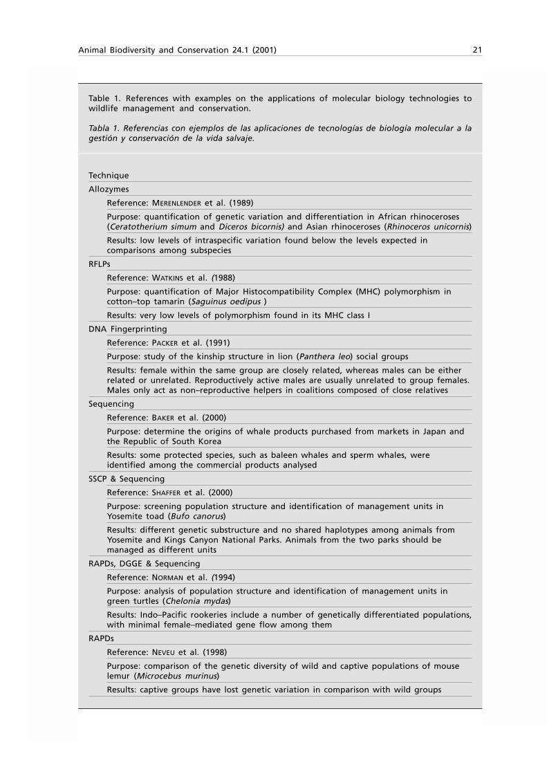
In this work, the wide variety of moleculartechniques available to support wildlifemanagement are reviewed and relevant examplesare provided in order to better understand whenthese techniques are used (table 1). The gap thatexists between technological possibilities andtheir use can thus be recognized to interpret thecomplexity of life is noted. Finally, molecularand non–molecular biologists are appealed tocollaborate in tracing the link between genesand adaptation so as to progress in many fieldsof life sciences including conservation biology.
Information contained in the DNA
Variation at a given DNA region is a consequenceof evolutionary forces such as mutation, selection,
genetic drift or recombination that have actedover the DNA and the species (GRAUR & LI, 2000;BERTRANPETIT, 2000). Within and across populationsand species the coalescense of genomic regionscan be traced back and the time when genes orgenome separated can be infered. Similarityrelationships between DNA segments can alsobe evaluated to infer relationships betweengenes, individuals and groups of individuals. Ifwe compare derivative characters with theirgeographic distribution, we can infer gene flowand colonisation events. In addition, thedistribution of alleles and the structure of thegenetic variation might be used to inferdemographic parameters such as population sizeand subdivisions (LUIKART & ENGLAND, 1999).
A wide variety of polymorphic DNA regionswith different mutation patterns and rates havebeen recognised. The choice of one or anotherregion will depend on the objectives of ourresearch. Most nuclear genome regions arediploid and inherited in an autosomal andcodominant fashion affected by recombination.They can code for RNA or be non–coding regions.In wildlife studies, microsatellites or STRs havebeen widely used (QUELLER et al., 1993; LUIKART &ENGLAND, 1999). They consist of a short string ofone to ten base pairs repeated in tandem andare dispersed throughout the genome. They arehighly polymorphic due to the variation in thenumber of repeat units and most behave asneutral markers. Minisatellites are also tandemlyrepeated strings of longer repeat units (JEFFREYS
et al., 1985). The number of repeats is inheritedand variable among individuals. This variabilitycan be detected with a probe that will attach toa single or several complementary DNA fragmentsamong all DNA fragments distributed throughan electrophoresis gel, providing a pattern ofbands for comparison.
Some microsatellites and minisatellites areassociated with mobile genetic elements, anotherDNA class that is currently gaining support forphylogenetic inference (BUCHANAN et al., 1999).These mobile or interspersed elements ofdifferent families and subfamilies occurthroughout the genome. Short InterspersedElements (SINEs) are excellent markers formolecular phylogeny since their integration at aparticular position in the genome can beconsidered an unambiguous derived homologouscharacter (TAKAHASHI et al., 1998). MitochondrialDNA (mtDNA) sequences include the other majorgroup of markers widely used in wildlife analyses(AVISE, 1994). Mitochondrial DNA is haploid,recombination free and maternally inherited. Ithas a low frequency of insertion, deletion andduplication events and an evolutionary rate 5–10times higher than single copy nuclear genes(BROWN et al., 1979).
Conclusions in animal conservation should besupported by the analyses of several independentdata sets (WAYNE et al., 1994). If we use different
Animal Biodiversity and Conservation 24.1 (2001) 21
Table 1. References with examples on the applications of molecular biology technologies towildlife management and conservation.
Tabla 1. Referencias con ejemplos de las aplicaciones de tecnologías de biología molecular a lagestión y conservación de la vida salvaje.
Technique
Allozymes
Reference: MERENLENDER et al. (1989)
Purpose: quantification of genetic variation and differentiation in African rhinoceroses(Ceratotherium simum and Diceros bicornis) and Asian rhinoceroses (Rhinoceros unicornis)
Results: low levels of intraspecific variation found below the levels expected incomparisons among subspecies
RFLPs
Reference: WATKINS et al. (1988)
Purpose: quantification of Major Histocompatibility Complex (MHC) polymorphism incotton–top tamarin (Saguinus oedipus )
Results: very low levels of polymorphism found in its MHC class I
DNA Fingerprinting
Reference: PACKER et al. (1991)
Purpose: study of the kinship structure in lion (Panthera leo) social groups
Results: female within the same group are closely related, whereas males can be eitherrelated or unrelated. Reproductively active males are usually unrelated to group females.Males only act as non–reproductive helpers in coalitions composed of close relatives
Sequencing
Reference: BAKER et al. (2000)
Purpose: determine the origins of whale products purchased from markets in Japan andthe Republic of South Korea
Results: some protected species, such as baleen whales and sperm whales, wereidentified among the commercial products analysed
SSCP & Sequencing
Reference: SHAFFER et al. (2000)
Purpose: screening population structure and identification of management units inYosemite toad (Bufo canorus)
Results: different genetic substructure and no shared haplotypes among animals fromYosemite and Kings Canyon National Parks. Animals from the two parks should bemanaged as different units
RAPDs, DGGE & Sequencing
Reference: NORMAN et al. (1994)
Purpose: analysis of population structure and identification of management units ingreen turtles (Chelonia mydas)
Results: Indo–Pacific rookeries include a number of genetically differentiated populations,with minimal female–mediated gene flow among them
RAPDs
Reference: NEVEU et al. (1998)
Purpose: comparison of the genetic diversity of wild and captive populations of mouselemur (Microcebus murinus)
Results: captive groups have lost genetic variation in comparison with wild groups
22 Domingo–Roura et al.
types of molecular data with different mutationrates we might be able to separate ancient fromrecent events. Another alternative is the comparisonof male–inherited DNA regions (i.e. non–recombining regions of the Y–chromosome) versusfemale–inherited DNA regions (such as mito-chondrial DNA) to understand the contribution ofeach sex in determining genetic diversity (MELNICK
& HOELZER, 1992; PÉREZ–LEZAUN et al., 1999). Thisanalysis can contribute to understanding how abalance is achieved between the proportion ofindividuals leaving the natal area and theproportion remaining philopatric to minimiseinbreeding and resource competition (GOMPER etal., 1998). To identify individuals, populations orspecies it is often recomended to work with geneticmarkers that are neutral and therefore goodindicators of ancestry or relationship (HEDRICK, 1996).
However, there is some concern regarding howneutral characters obtained from non–codingregions reflect the diversity of functional attributes(WILLIAMS et al., 1994; LYNCH, 1996).
Technology available
The main goal of molecular techniques is todetect the variation in DNA sequences, directlythrough sequencing or indirectly through othermethods sensitive to sequence variations. Thisvariation can be detected using a wide range oftechniques. A first group of techniques includingisozymes and restriction fragment lengthpolymorphisms (RFLP) is based on the differentialmobility of proteins and DNA fragmentsrespectively (due to their different charge or size)
Technique
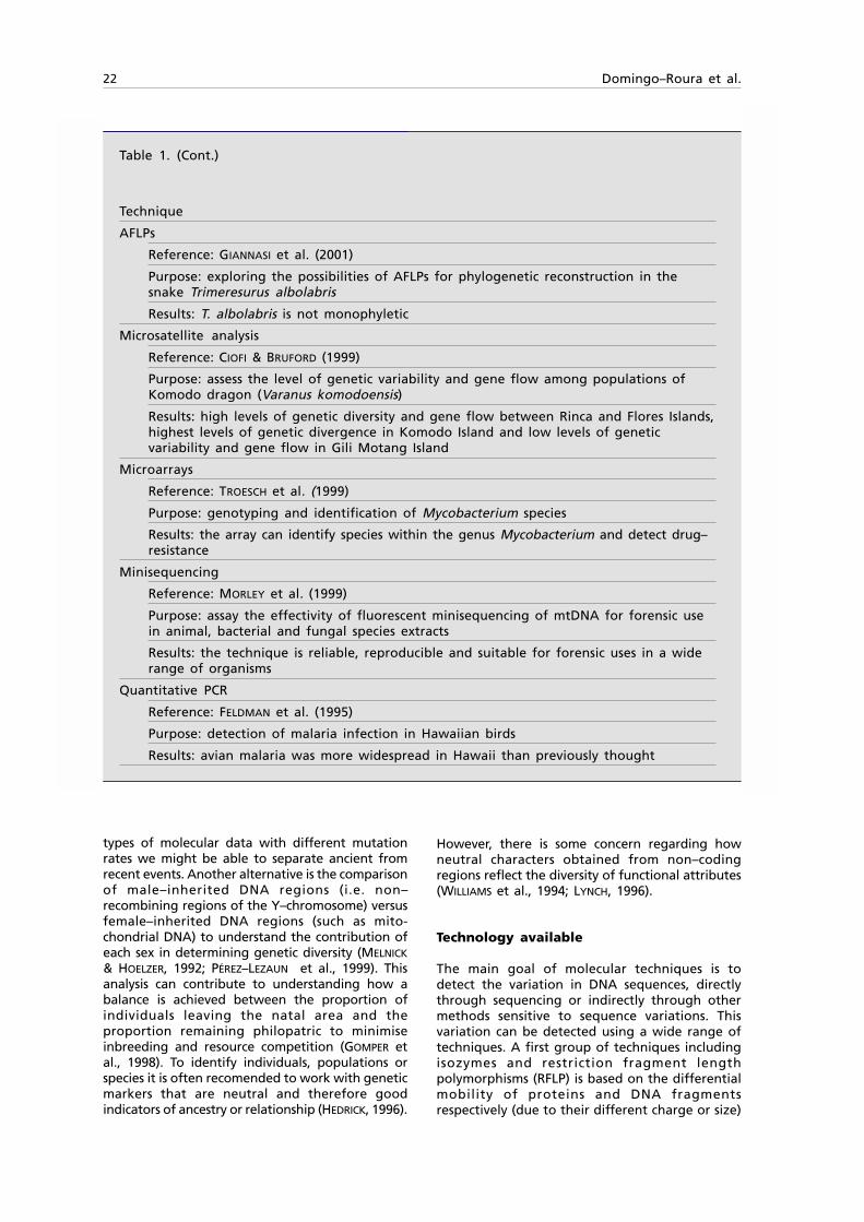
AFLPs
Reference: GIANNASI et al. (2001)
Purpose: exploring the possibilities of AFLPs for phylogenetic reconstruction in thesnake Trimeresurus albolabris
Results: T. albolabris is not monophyletic
Microsatellite analysis
Reference: CIOFI & BRUFORD (1999)
Purpose: assess the level of genetic variability and gene flow among populations ofKomodo dragon (Varanus komodoensis)
Results: high levels of genetic diversity and gene flow between Rinca and Flores Islands,highest levels of genetic divergence in Komodo Island and low levels of geneticvariability and gene flow in Gili Motang Island
Microarrays
Reference: TROESCH et al. (1999)
Purpose: genotyping and identification of Mycobacterium species
Results: the array can identify species within the genus Mycobacterium and detect drug–resistance
Minisequencing
Reference: MORLEY et al. (1999)
Purpose: assay the effectivity of fluorescent minisequencing of mtDNA for forensic usein animal, bacterial and fungal species extracts
Results: the technique is reliable, reproducible and suitable for forensic uses in a widerange of organisms
Quantitative PCR
Reference: FELDMAN et al. (1995)
Purpose: detection of malaria infection in Hawaiian birds
Results: avian malaria was more widespread in Hawaii than previously thought
Table 1. (Cont.)
Animal Biodiversity and Conservation 24.1 (2001) 23
in an electrophoretic field (MÜLLER–STARK, 1998;BRETTSCHNEIDER, 1998). Hybridisation between alabeled DNA fragment or probe and a target DNAis the principle involved in many other techniques(SAMBROOK et al., 1989).
With the discovery of the polymerase chainreaction (PCR) (SAIKI et al., 1988), a new wave ofmolecular techniques appeared. One importantadvantage of the PCR is that a given DNA fragmentcan be isolated and copied millions of timesreliably and quickly using temperature cycles anda thermally stable polymerase. This allows the useof minute amounts of DNA in molecular studies,such as those obtained from biological remnantsobtained non-invasively (WOODRUFF, 1993).
Sequencing
The complete sequencing of the whole genomeis the most detailed method to detect geneticvariability. However, sequencing completegenomes is tedious and expensive and moststudies rely on the sequencing of a minute portionof the genome and the assumption that variationwithin the fragment sequenced represents thevariation along the whole genome. Sequencingof PCR products of up to several hundred basepairs is a widely used methodology in life sciences.During the sequencing reaction of a PCR product,a large number of fragments differing by anucleotide in length and with the last baselabelled with a specific fluorochrome dependingon its identity are obtained (WEAVER & HEDRICK,1992). When these sequencing products ofdifferent length are electrophoresed in a DNAsequencer, the ladder of fluorochrome signalsobtained will indicate the nucleotide sequenceof the PCR product under analysis. It is commonpractice to deposit the sequences obtained inpublic databases, facilitating both the comparisonand complementation of one’s own data withthe data from the same or other species obtainedby other researchers.
Sequencing can be combined with othermethods to reduce its cost. A first group of PCR–based methods (Heteroduplex analysis, SingleStrand Conformation Polymorphisms, DenaturingGradient Gel Electrophoresis and TemperatureGradient Gel Electrophoresis) consists of screeningtechniques for detecting sequence variation in PCRproducts of identical sizes, without the need to gothrough sequencing. These protocols are based onthe physical behaviour of DNA during electro–phoresis in acrylamide gels. The use of thesemethods is adequate when dealing with a largenumber of samples and when alleles are shared bymany individuals (LESSA & APPLEBAUM, 1993).
Heteroduplex analysis
Heteroduplex analysis starts with the denaturingof the PCR product at 95ºC and its subsequentrenaturation before electrophoresis (LESSA &
APPLEBAUM, 1993). Using this technique it ispossible to distinguish between homozygous andheterozygous DNA fragments. If a samplecontains two different alleles, heteroduplexmolecules (hybrids of the two strands belongingto different alleles) are obtained. Since theseheteroduplexes have one or more mismatches intheir double strands, they migrate onto the gelmore slowly than the homoduplex moleculesobtained from the hybridization of strandscontaining the same allele.
Single–Strand Conformation Polymorphism (SSCP)
SSCP is a simple and fast method for screeningDNA fragments for nucleotide sequence poly-morphisms. PCR products that have beendenatured by temperature and/or chemicals areloaded and run onto a non–denaturing polya-crylamide gel. The electrophoretic mobility ofeach single–stranded DNA fragment depends onits secondary structure, which in turn depends onits nucleotide sequence (JORDAN et al., 1998). SSCPcan distinguish DNA fragments that differ only byone base-pair substitution in a fragment of up toseveral hundred nucleotides (ORITA et al., 1989).
Denaturing Gradient Gel Electrophoresis (DGGE) andTemperature Gradient Gel Electrophoresis (TGGE)
DGGE and TGGE work over double stranded DNA.In these methods, PCR products are loaded onto apolyacrylamide gel and run in a linear gradient ofconcentration of denaturing solvents (urea,formamide) or temperature respectively (LESSA &APPLEBAUM, 1993). The point along the gradientwhere the DNA fragment is partially denatured iscalled the melting point. This point depends onthe overall base composition and the interactionsacross the molecule and can be modified by pointmutations that will be reflected in the gel.
Randomly Amplified Polymorphic DNAs (RAPDs) andAmplified Fragment Length Polymorphisms (AFLPs)
The principle of the RAPD technique is thesimultaneous amplification of DNA regions byusing a single randomly chosen primer whichacts as both forward and reverse (GROSBERG et.al., 1996). This primer is able to hybridise withmany sites of target DNA, but amplification onlyoccurs when the primer anneals at two sites onopposite strands separated by a reasonabledistance for the PCR to work (20 to 2000 bp).These fragments are then separated in anelectrophoresis gel and stained with chemicalssuch as ethidium bromide or silver nitrate. Thegels can be scored as the presence or absence ofa band of a specific molecular weight. Bands ofdifferent sizes usually represent independent loci.RAPDs are treated as neutral and anonymousmarkers, can be generated quickly and a largenumber of individuals can be processed in a

24 Domingo–Roura et al.
short time. However, results are difficult torepeat, a band can contain more than oneamplification product that can not be distinguish-ed and it is difficult to estimate allelic frequenciesbecause homozygotes can not be distinguishedfrom heterozygotes. In addition, it is sometimesdifficult to know whether the variation is neutralor whether it follows Mendelian inheritance.
In AFLPs, genomic DNA is digested withrestriction enzymes and the goal is to reduce thecomplexity of the initial mixture of fragments.To achieve this reduction a subset of fragmentsis biotinylated and selected by union tostreptavidin-coated paramagnetic beads (sincebiotine binds covalently to streptavidine)(MATTHES et al., 1998). The unbound fragmentsare washed and discarded. A subset of thebiotinylated fragments is then amplified by PCRto further reduce complexity. Finaly, PCR productsare analysed by denaturing polyacrilamide gelelectrophoresis and revealed by autoradiography.AFLPs are more informative and easier toreproduce than RAPDs.
Automation required
Automation is a key issue in molecular biologyand the machinery used in the automated analysesof humans and model animals is later adapted towildlife research. Automated procedures arecurrently used for standard procedures such asDNA isolation or library construction and spottingbut also for the fast scoring of genetic variabilityamong individuals with technologies such asmicroarrays or quantitative PCR.
Microsatellite multiplexing
Several microsatellite loci can be amplified in asingle PCR reaction containing different primers(GILL et al., 1995). The primers are labeled withdifferent fluorochromes and amplify fragmentsof different lengths. When the multiplex PCRreaction is run in an automated sequencer it ispossible to sequentially detect the length of thedifferent PCR products corresponding to thealleles of the different microsatellite loci.
DNA array technology
A DNA array consists of up to thousands of DNAstrings attached in order over a solid support(SOUTHERN et al., 1999). An unknown sample ispassed over the array and it will hybridize uponthe immobilised probes when finding acomplementary sequence. The reverse is alsopossible when a known probe hybridises uponunknown immobilised fragments. The fullmicroarray equipment consists of a machine toproduce the array and a machine with afluorescence laser scanner to read the signal andtranslate this signal to a computer. The great
advantage of microarray technology is that itallows the fast detection of sequence informationfrom a large number of loci or individuals at thesame time. Paradoxically, one of the mainproblems encountered with microarray technol-ogy is that it generates such a large amount ofinformation that results are often difficult tointerpret. Microarrays are used, for instance, tomonitor RNA expression and gene function (DE
SAIZIEU et al., 1997; WODICKÁ et al., 1997; CHO etal., 1998) or to detect single nucleotidepolymorphisms (SNPs) (CHAKRAVARTI, 1999). Allstudies published used model species and, as faras we know, no study using microarraytechnology has yet been performed in any specieswith a conservation perspective.
Minisequencing
The technique consists of a PCR–based mini-sequencing reaction where the polymerase addsa single nucleotide. Primers finalise just beforethe polymorphic position that needs to beinterrogated. The polymerase extends the firstbase position after the primer with labelled newnucleotides and the identity of the incorporatednucleotide can be determined with an automatedsequencer. Several reactions can be performedsimultaneously with primers of different sizes. Itis also possible to conduct a minisequencingreaction in a DNA array (HACIA, 1999; RAITIO etal., 2001).
Quantitative PCR
Quantitative PCR consists of a reaction thatdetects and quantifies nucleic acid sequenceseither as a final product or while the reaction isbeing produced. The protocol is based on thedetection of fluorescence emitted by thedegradation of an internal labelled oligocomplementary to our sample when the PCRproceeding is being produced. The outcome isthe quantification of a PCR product that can beused in gene expression studies (DE KOK et al.,2000), to evaluate viral load (LIMAYE et al., 2001),and to detect transgenes (FAIRMAN et al., 1999),duplications and deletions (AARSKOG & VEDELER,2000; WILKE et al., 2000) and SNPs (BREEN et al.,2000). Quantitative PCR and minisequencing canbe cheaper alternatives to microarrays for thestudy of SNPs if a moderate number of SNPs andindividuals are to be analysed.
Looking for the link between molecular dataand conservation
Technological resources are available, but theconnection between molecular variability andthe needs of endangered species is notstraightforward. Gene dynamics is complex, mostphenotypic characters are multigenic, and the
Animal Biodiversity and Conservation 24.1 (2001) 25
genetic machinery is loaded with complicatedgene interactions and epistases (HEDRICK, 1996).More than one protein can be translated from asingle gene due to alternative splicing (GRAUR &LI, 2000). Genetic linkage can also mask the roleof important genes. In addition, the relationshipbetween gene and environment is often difficultto discern (FALCONER, 1989). All levels of lifeexpression and population processes are complexand manifold and quick fixes to animalmanagement questions based on simplemolecular biology analyses should be avoided.
Genetic diversity has been linked to speciesrichness and to better chances to cope efficientlywith enviromental change (HEDRICK & MILLER, 1992;O’BRIEN et al., 1985). Consanguineous matingspromote the existence of deleterious genes inhomozygosis, which can be detrimental forsurvival and reproduction. In theory, fitness insmall populations will decline due to theaccumulation of detrimental mutations (LYNCH
et al., 1995a, 1995b). However, the importanceof genetic variability for species survival is notclearly defined. In practice, at least somepopulations can survive in spite of having lowgenetic variability (e.g cheetahs [Acinonyxjubatus] [O´BRIEN et al., 1987], mole–rats[Heterocephalus glaber] [FAULKES et al., 1990;REEVE et al., 1990] and Eurasian badgers [Melesmeles] [DOMINGO–ROURA, 2000]). The empiricalrelationship between genetic distance and fitnessis likely to be species–specific and is unlikely tobe linear (LYNCH, 1991).
In the past, considerable effort has beendevoted to describe key demographic numbersrequired to maintain the necessary geneticvariability needed for species survival (SOULÉ, 1987).However, key numbers are unlikely to beapplicable across populations or habitats. In thelast decade, polemics concerning the existence ofkey numbers for survival have often given way toother discussions, not often based on molecularinformation. Within species, conservationstrategies have been proposed on the basis of theexistence of Evolutionary Significant Units (ESUs)which have been defined as population units thatmerit separate management and have high priorityfor conservation (RYDER, 1986). The use of ESUs inconservation has signified an upgrade fromprevious strategies that only gave importance toindividual numbers without considering dif–ferences among individuals of the same species.However, a compromise has not yet been reachedregarding the relative importance of ecologicaladaptation and genetic variability to determinethese units (MACE et al., 1996). Furthermore, theinadequacies of the dichotomy implied in the ESUconcept in a world ruled by a continuum ofpopulation differentiation have been noted(CRANDALL et al., 2000).
Across species, molecular techniques are alsoat the base of new strategies to support anintegrated approach to conservation, focusing on
the preservation of evolutionary diversity insteadof focusing on species number (MAY, 1990; MACE etal., 1996) or single–species management. In thiscase, molecular data should play a predominantrole in the selection of areas that containevolutionarily distant lineages and areas ofpotential evolutionary novelty, such as multispeciescontact zones (MORITZ & FAITH, 1998). The protectionof these areas is likely to preserve large amountsof evolutionary heritage and will maximise theevolutionary–response potential to perturbations(PETIT et al., 1998). In fact, discussing key numbersand even single–species conservation strategiesmight be naif in the face of the immense complexityof nature.
Looking for the link between gene andfunction
The rapid development of molecular geneticsfor biomedical and industrial purposes facilitatesthe access to molecular technology. Resolution isalso increased with new techniques and a highernumber of markers. The increase in the numberof markers known in any species means greaterprobabilities to detect major loci that influencequantitative traits.
As we learn more about DNA, molecularinformation will be better understood when usedin combination with physiological, demographic,ecological and behavioural data collected in thefield (HAIG, 1998). Data can originate from anyparameter that can group individuals in relation totheir evolutionary origin and/or ecological needs. Inanimal conservation it is not enough to understandand describe molecular variation or even ecologicaland demographic characteristics using moleculartools. We need to find loci that have variants thatare responsible for low fitness and survival.Ecologically relevant heritable traits might need tobe emphasised (CRANDALL et al., 2000).
Nevertheless, fitness measurement might bedifficult in endangered species. Since a selectivedifference smaller than the reciprocal of twicethe effective population size (1/2Ne) is effectivelyneutral (KIMURA, 1979), small selective differencesare unlikely to be of adaptive significance in mostendangered species. A further complication arisesfrom the possible differences between formerand current selection and adaptation processes.The habitat currently used by a rare species canbe marginal and might no longer reflect theenvironmental condition in which the traitsevolved (JOHNSON et al., 2000). This is especiallytrue for carnivores since human expansion hasconsiderably altered their distribution and ecology(GRIFFITHS & THOMAS, 1993).
To unravel the link between gene and functionor adaptation is not a goal exclusive toconservation genetics. For instance, to clarifythe function of genes that are likely to beresponsible for diseases is a major enterprise in
26 Domingo–Roura et al.
current biomedicine. Since the link betweengenotype and phenotype is still widely unknown,the potential of molecular biology in wildlifemanagement and conservation is still at a veryearly stage. At this point, still far from applyingthe functional interpretation of genetic variationto wild species, to advance the understanding ofenhanced fitness and the evolutionary paths ofphysiological systems, several approaches can beconsidered. The genetic structure of a populationcan be examined to identify physiologicalphenotypes with highest fitness. Interindividualvariation can be used to identify physiological,biochemical and molecular characters thatcorrelate with fitness and survival. Comparativestudies to trace the evolution of characters withparticular phylogenies can also be useful tounderstand the role of these characters inradiation and extinction. Other importantapproaches are the experimental manipulationof genes through genetic engineering, and theexperimental manipulation of the environmentthrough controlled laboratory conditions andimposed selection pressures. Even if many wildlifebiologists dislike strategies such as geneticengineering, manipulative experiments andkeeping animals in captivity, scientific progresswill certainly be slower and may be incompletewithout using these more aggressive approaches.Unfortunately, economic progress and habitatdeterioration is unlikely to be slow or incomplete.
More data, new trends
The current trend towards automation androbotisation can create important shifts in thefocus of wildlife research. Highly automatedlaboratories are expensive but open the possibilityof subcontracting services to specialised companieswhich can offer the same protocols than a universityresearcher could conduct in his or her laboratory ina cheaper, faster and often more reliable way.Some biotechnology companies are even taking afurther step and sequencing interesting regions,such as regions responsible for main humandiseases, in a large number of individuals, with noprevious order, and selling the use of the sequencesas a product. Not only this, but since many journalsand common sense require sequence data bedeposited in public databases, the amount ofsequence data is increasing steadily. Laboratorytechnicians can be accurately trained to developprotocols complementary to the services offeredby specialised companies. The trend is switchingfrom young researchers who can run molecularprotocols towards young researchers who cananalyse molecular data generated by others. Evenif this high throughput trend makes better sensewhen considering human molecular biology, theamount of DNA sequences from wild animals thatcan be found in public databases is already amazing.In addition, the dog has been suggested to be a
good model for identifying the genetic control ofmorphologic characteristics in mammals (WAYNE &OSTRANDER, 1999). The sequencing of wholegenomes for conservation purposes has not yetbegun. However the proposal to start sequencingthe genome of chimpanzees or macaques tounderstand genetic and functional differencesbetween humans and other primates (MCCONKEY &VARKI, 2000) is likely to see the light soon.
When we leave molecular dynamics and startdealing with gene–environment interactions andadaptive characters, knowledge in other biologicalsciences such as ecology, zoology and behaviourbecomes essential. Molecular differences have tobe contrasted against non–molecular data in, forinstance, geography, behaviour, morphology, andfunction. Applications in animal conservation onlymake sense when compared to field data, even ifinitially these data are just the species name (notalways easy to determine) and the geographicorigin of a sample. Accurate field data can alsoconsiderably improve the resolution of experiments.As noted by MACE et al. (1996), many studies thatattempt to reconstruct familial relationships frommolecular data are unable to resolve therelationship fully, even if this might have beenfeasible had observations been made on thebreeding population to reduce the set ofuncertainties for analysis.
It would be great for the progress of biologicalsciences and, thus, for animal conservation ifsamples and field data could be as easilyaccessible as DNA sequences to the general public.This lack of availability of samples and datacreates drawbacks such as the need to spendlong periods of time searching for the materialrequired, for instance, to review the phylogenyof a doubtful taxon. This time could be devotedto more fruitful tasks if the material andaccompanying data were readily available frommuseums and other, often public, specializedinstitutions. In this regard, the link betweennon–molecular and molecular databases isbecoming an urgent need.
Successful experiments should be based in thefuture on a justified trust and collaborationbetween field and laboratory biologists. Themolecular trend of research during recent yearsand the ease and speed with which moleculardata can sometimes be published might haveworked against the funding of field projects andof projects in many other areas of biology crucialfor conservation biology. This trend will certainlyneed to be reviewed in the future when we tryto translate molecular data back to nature.
Acknowledgements
We thank Francesc Calafell and Luis Pérez–Juradofor their helpful comments to improve themanuscript. J. Marmi and J. F. López–Giráldezare supported by scholarships from the
Animal Biodiversity and Conservation 24.1 (2001) 27
Departament d’Universitats, Recerca i Societatde la Informació, Generalitat de Catalunya (Refs.2000FI–00698 and 2001FI–00625 respectively).
References
AARSKOG, N. K. & VEDELER, C. A., 2000. Real–timequantitative polymerase chain reaction. A newmethod that detects both the peripheralmyelin protein 22 duplication in Charcot–Marie–Tooth type 1A disease and theperipheral myelin protein 22 deletion inhereditary neuropathy with liability to pressurepalsies. Hum. Genet., 107(5): 494–498.
AVISE, J. C., 1994. Molecular markers, natural historyand evolution. Ed. Chapman and Hall, London.
BAKER, C. S., LENTO, G. M., CIPRIANO, F. & PALUMBI,S. R., 2000. Predicted decline of protectedwhales based on molecular genetic monitoringof Japanese and Korean markets. Proc. R. Soc.Lond. B. Biol. Sci., 267: 1,191–1,199.
BEGON, M., HARPER, J. L. & TOWNSEND, C. R. (Eds.),1999. Ecología. Individuos, poblaciones ycomunidades. Ed. Omega, Barcelona.
BERTRANPETIT, J., 2000. Genome, diversity, andorigins: the Y chromosome as a storyteller.Proc. Natl. Acad. Sci. USA, 97: 6,927–6,929.
BREEN, G., HAROLD, D., RALSTON, S., SHAW, D. & ST
CLAIR, D., 2000. Determining SNP allelefrequencies in DNA pools. Biotechniques, 28:464–466, 468, 470.
BRETTSCHNEIDER, R., 1998. RFLP analysis. In:Molecular tools for screening biodiversity: 83–85 (A. Karp, P. G. Isaac & D. S. Ingram, Eds.).Ed. Chapman & Hall, Cambridge.
BROWN, W. M., GEORGE, M. JR. & WILSON, A. C., 1979.Rapid evolution of animal mitochondrial DNA.Proc. Nat. Acad. Sci. USA, 76: 1,967–1,971.
BUCHANAN, F., CRAWFORD, A., STROBECK, C., PALSBOLL,P. & PLANTE, Y., 1999. Evolutionary applicationsof MIRs and SINEs. Anim. Genet., 30: 47–50.
CAUGHLEY, G., 1994. Directions in conservationbiology. J. Anim. Ecol., 63: 215–244.
CHAKRAVARTI, A., 1999. Population genetics-making sense out of sequences. Nat. Genet.Suppl., 21: 56–60.
CHO, R. J., FROMONT–RACINE, M., WODICKÁ, L.,FEIERBACH, B., STEARN, T., LEGRAIN, P., LOCKHART,D. J. & DAVIS, R. W., 1998. Parallel analysis ofgenetic selections using whole genomeoligonucleotide arrays. Proc. Natl. Acad. Sci.USA, 95: 3,752–3,757.
CIOFI, C. & BRUFORD, M. W., 1999. Genetic structureand gene flow among Komodo dragonpopulations inferred by microsatellite locianalysis. Mol. Ecol., 8: S17–S30.
CRANDALL, K. A., BININDA–EMONDS, O. R. P., MACE,G. M. & WAYNE, R. K., 2000. Consideringevolutionary processes in conservation biology.Trends Ecol. Evol., 15: 290–295.
DE KOK, J. B., RUERS, T. J., VAN MUIJEN, G. N., VAN
BOKHOVEN, A., WILLEMS, H. L. & SWINKELS, D. W.,
2000. Real–time quantification of humantelomerase reverse transcriptase mRNA intumors and healthy tissues. Clin. Chem., 46:313–318.
DE SAIZIEU, A., VANKAN, P., VOCKLER, C. & VAN LOON,A. P., 1997. The trp RNA–binding attenuationprotein (TRAP) regulates the steady–state levelsof transcripts of the Bacillus subtilis folateoperon. Microbiology, 143: 979–989.
DOMINGO–ROURA, X., 2000. Biochemical andmolecular ecology of Eurasian badgers, Melesmeles, and Japanese macaques, Macaca fuscata:Nutritional and reproductive requirements. Ph.D. Thesis, Univ. of Oxford.
EHRLICH, P. R. & WILSON, E. O., 1991. Biodiversitystudies: science and policy. Science, 253: 758–761.
FAIRMAN, J., ROCHE, L., PIESLAK, I., LAY, M., CORSON,S., FOX, E., LUONG, C., KOE, G., LEMOS, B., GROVE,R., FRADKIN, L. & VERNACHIO, J., 1999.Quantitative RT–PCR to evaluate in vivoexpression of multiple transgenes using acommon intron. Biotechniques, 27: 566–570,572–574.
FALCONER, D. S., 1989. Introduction to quantitativegenetics. 3rd Edition. Ed. Longman Scientificand Technical, Hong Kong.
FAULKES, C. G., ABBOTT, D. H. & MELLOR, A. L.,1990. Investigation of genetic diversity in wildcolonies of naked mole–rats (Heterocephalusglaber) by DNA fingerprinting. J. Zool., Lond.,221: 87–97.
FELDMAN, R. A., FREED, L. A. & CANN, R. L., 1995. APCR test for avian malaria in Hawaiian birds.Mol. Ecol., 4: 663–673.
GIANNASI, N., THORPE, R. & MALHOTRA, A., 2001.The use of amplified fragment lengthpolymorphism in determinng species trees atfine taxonomic levels: analysis of a medicallyimportant snake, Trimeresurus albolabris. Mol.Ecol., 10: 419–426.
GILL, P., KIMPTON, C. P., URQUHART, A., OLDROYD, N.,MILLICAN, E. S., WATSON, S. K. & DOWNES, T. J.,1995. Automated short tandem repeat (STR)analysis in forensic casework – a strategy forthe future. Electrophoresis, 16: 1,543–1,552.
GOMPER, M. E., GITTLEMAN, J. L. & WAYNE, R. K.,1998. Dispersal, philopatry, and geneticrelatedness in a social carnivore: comparingmales and females. Mol. Ecol., 7: 157–163.
GRAUR, D. & LI, W. H., 2000. Fundamentals ofmolecular evolution. 2nd ed. Ed. Sinauer,Sunderland, Massachusetts.
GRIFFITHS, H. I. & THOMAS, D. H., 1993. The status ofthe badger Meles meles L., 1758 (Carnivora,Mustelidae) in Europe. Mammal Rev., 23: 17–58.
GROSBERG, R., LEVITAN, D. & CAMERON, B., 1996.Characterization of genetic structure andgenealogies using RAPD–PCR markers: arandom primer for the novice and nervous. In:Molecular zoology: advances, strategies andprotocols: 67–100 (J. D. Ferraris & S. R. PalumbiEds.). Ed. Wiley–Liss, New York.
HACIA, J. G., 1999. Resequencing and mutational

28 Domingo–Roura et al.
analysis using oligonucleotide microarrays. Nat.Genet. Suppl., 21: 42–47.
HAIG, S. M., 1998. Molecular contributions toconservation. Ecology, 79: 413–425.
HEDRICK, P. W., 1996. Conservation genetics andmolecular techniques: a perspective. In:Molecular genetics approaches in conservation:459–477 (T. B. Smith & R. K. Wayne, Eds.).Oxford University Press, Oxford.
HEDRICK, P. W. & MILLER, P. S., 1992. Conservationgenetics: techniques and fundamentals. Ecol.Appl., 2: 30–46.
JEFFREYS, A. J., WILSON, V. & THEIN, S. L., 1985.Hypervariable "minisatellite" regions in humanDNA. Nature, 314: 67–73.
JOHNSON, D. D. P., MACDONALD, D. W. & DICKMAN,A. J., 2000. An analysis and review of modelsof the sociobiology of the Mustelidae. MammalRev., 30: 171–196.
JORDAN, W., FOLEY, K. & BRUFORD, M., 1998.Single–strand conformation polymorphism(SSCP) analysis. In: Molecular tools forscreening biodiversity: 152–156 (A. Karp, P.G. Isaac & D. S. Ingram, Eds.). Ed. Chapman& Hall, Cambridge.
KIMURA, M., 1979. The neutral theory ofmolecular evolution. Sci. Am., 241: 94–104.
LESSA, E. P. & APPLEBAUM, G., 1993. Screeningtechniques for detecting allelic variation inDNA sequences. Mol. Ecol., 2: 119–129.
LIMAYE, A. P., JEROME, K. R., KUHR, C. S., FERRENBERG,J., HUANG, M. L., DAVIS, C. L., COREY, L. & MARSH,C. L., 2001. Quantitation of BK virus load inserum for the diagnosis of BK virus–associatednephropathy in renal transplant recipients. J.Infect. Dis., 183: 1,669–1,672.
LUIKART, G. & ENGLAND, P. R., 1999. Statisticalanalysis of microsatellite DNA data. TrendsEcol. Evol., 14: 253–256.
LYNCH, M., 1991. The genetic interpretation ofinbreeding and outbreeding depression.Evolution, 45: 622–629.
– 1996. A quantitative genetic perspective onconservation issues. In: Conservation genetics:case histories from nature: 471–501 (J. C. Avise& J. L. Hamrick, Eds.). Ed. Chapman and Hall,New York.
LYNCH, M., CONERY, J. & BURGER, R., 1995a.Mutational meltdowns in sexual populations.Evolution, 49: 1,067–1,080.
– 1995b. Mutational accumulation and theextinction of small populations. Am. Nat., 146:489–518.
MACE, G. M., SMITH, T. B., BRUFORD, M. W. & WAYNE,R. K., 1996. An overview of the issues. In:Molecular genetic approaches in conservation:3–21 (T. B. Smith & R. K. Wayne, Eds.). OxfordUniversity Press, New York.
MATTHES, M. C., DALY, A. & EDWARDS, K., 1998.Amplified fragment lenght polymorphism(AFLP). In: Molecular tools for screeningbiodiversity: 183–190 (A. Karp, P. G. Isaac & D. S.Ingram, Eds.). Ed. Chapman & Hall, Cambridge.
MAY, R., 1990. Taxonomy as destiny. Nature, 347:129–130.
MCCONKEY, E. H. & VARKI, A., 2000. A primategenome project deserves high priority. Science,289: 1,295–1,296.
MELNICK, D. J. & HOELZER, G. A., 1992. Differencesin male and female macaque dispersal leadsto contrasting distributions of nuclear andmitochondrial DNA variation. Int. J. Primatol.,13: 379–393.
MERENLENDER, A. M., WOODRUFF, D. S., RYDER, O.A., KOCK, R. & VAHALA, J., 1989. Allozymevariation and differentiation in African andIndian rhinoceroses. J. Hered., 80: 377–382.
MORITZ, C. & FAITH, D. P., 1998. Comparativephylogeography and the identification ofgenetically divergent areas for conservation.Mol. Ecol., 7: 419–429.
MORLEY, J. M., BARK, J. E., EVANS, C. E., PERRY, J. G.,HEWITT, C. A. & TULLY, G., 1999. Validation ofmitochondrial DNA minisequencing for forensiccasework. Int. J. Legal Med., 112: 241–248.
MÜLLER–STARCK, G., 1998. Isozymes. In: Moleculartools for screening biodiversity: 73–82 (A. Karp,P. G. Isaac & D. S. Ingram, Eds.). Ed. Chapman& Hall, Cambridge.
NEGRO, J. J. & TORRES, M. J., 1999. Geneticvariability and differentiation of two beardedvulture Gypaetus barbatus and implicationsfor reintroduction projects. Biol. Conserv., 87:249–254.
NEVEU, H., HAFEN, T., ZIMMERMANN, E. & RUMPLER, Y.,1998. Comparison of the genetic diversity ofwild and captive groups of Microcebus murinususing the random amplified polymorphic DNAmethod. Folia Primatol., 69: 127–135.
NORMAN, J. A., MORITZ, C. & LIMPUS, C. J., 1994.Mitochondrial DNA control region poly-morphisms: genetic markers for ecologicalstudies of marine turtles. Mol. Ecol., 4: 363–373.
O´BRIEN, S. J., ROELKE, M. E., MARKER, L., NEWMAN,A., WINKLER, C. A., MELTZER, D., COLLY, L.,EVERMANN, J. F., BUSH, M. & WILDT, D. E., 1985.Genetic basis for species vulnerability in thecheetah. Science, 227: 1,428–1,434.
O´BRIEN, S. J., WILDT, D. E., BUSH, M., CARO, T. M.,FITZGIBBON, C., AGGUNDEY, I. & LEAKEY, R. E.,1987. East African cheetahs: evidence for twopopulation bottlenecks? Proc. Natl. Acad. Sci.USA, 84: 508–511.
ORITA, M., IWAHANA, H., KANAZAWA, H., HAYASHI, K.& SEKIYA, T., 1989. Detection of polymorphismsof human DNA by gel electrophoresis andsingle–strand conformation polymorphisms.Proc. Natl. Acad. Sci. USA, 86: 2,766–2,770.
PACKER, C., GILBERT, D. A., PUSEY, A. E. & O´BRIEN, S.J., 1991. A molecular genetic analysis of kinshipand cooperation in African lions. Nature, 351:562–565.
PÉREZ–LEZAUN, A., CALAFELL, F., COMAS, D., MATEU,E., BOSCH, E., MARTÍNEZ–ARIAS, R., CLARIMÓN, J.,FIORI, G., LUISELLI, D., FACCHINI, F., PETTENER, D. &BERTRANPETIT, J., 1999. Sex–specific migration

Animal Biodiversity and Conservation 24.1 (2001) 29
patterns in Central Asian populations revealedby the analysis of Y–chromosome STRs andmtDNA. Am. J. Hum. Genet., 65: 208–219.
PETIT, R. J., EL MOUSADIC, A. & PONS, O., 1998.Identifying populations for conservation onthe basis of genetic markers. Conserv. Biol.,12: 844–855.
QUELLER, D. C., STRASSMANN, J. E. & HUGHES, C. R.,1993. Microsatellites and kinship. Trends Ecol.Evol., 8: 285–288.
RAITIO, M., LINDROOS, K., LAUKKANEN, M., PASTINEN, T.,SISTONEN, P., SAJANTILA, A. & SYVANEN, A. C., 2001.Y–chromosomal SNPs in finno–ugric–speakingpopulations analyzed by minisequencing onmicroarrays. Genome Res., 11: 471–482.
REEVE, H. K., WESTNEAT, D. F., NOON, W. A., SHERMAN,P. W. & AQUADRO, C. F., 1990. DNA "finger–printing" reveals high levels of inbreeding incolonies of the eusocial nacked mole–rat. Proc.Natl. Acad. Sci. USA, 87: 2,496–2,500.
RYDER, O. A., 1986. Species conservation andsystematics: the dilemma of subspecies. TrendsEcol. Evol., 1: 9–10.
SAIKI, R. K., GELFAND, D. H., STOFFEL, S., SCHARF, S.J., HIGUCHI, R., HORN, G. T., MULLIS, K. B. &ERLICH, H. A., 1988. Primer–directed enzymaticamplification of DNA with a thermostableDNA polymerase. Science, 239: 487–491.
SAMBROOK, J., FRITSCH, E. F. & MANIATIS, T., 1989.Molecular cloning. A laboratory manual, 2nd
edition. Ed. Cold Spring Harbor LaboratoryPress, New York.
SHAFFER, H. B., FELLERS, G. M., MAGEE, A. & VOSS, S.R., 2000. The genetics of amphibian declines:population substructure and moleculardifferentiation in the yosemite toad, Bufocanorus (Anura, Bufonidae) based on single–strand conformation polymorphism analysis(SSCP) and mitochondrial DNA sequence data.Mol. Ecol., 3: 245–257.
SOULÉ, M. E. (Ed.), 1987. Viable populations forconservation. Ed. Cambridge University Press,Cambridge.
SOUTHERN, E., MIR, K. & SHCHEPINOV, M., 1999.Molecular interactions on microarrays. Nat.Genet., 21: 5–9.
TABERLET, P. & BOUVET, J., 1994. Mitochondrial
DNA polymorphism, phylogeography, andconservation genetics of the brown bearUrsus arctos in Europe. Proc. R. Soc. Lond.,255: 195–200.
TAKAHASHI, K., TERAI, Y., NISHIDA, M. & OKADA, N.,1998. A novel family of short interspersedrepetitive elements (SINEs) from cichlids: thepatterns of insertion of SINEs at orthologousloci support the proposed monophyly of fourmajor groups of cichlid fishes in LakeTanganika. Mol. Biol. Evol., 15: 391–407.
TROESCH, A., NGUYEN, H., MIYADA, C. G, DESVARENNE,S., GINGERAS, T. R, KAPLAN, P. M., CROS, P. &MABILAT, C., 1999. Mycobacterium speciesidentification and rifampin resistance testingwith high–density DNA probe arrays. J. Clin.Microbiol. 37: 49–55.
WATKINS, D. I., HODI, F. S. & LETVIN, N. L., 1988. Aprimate species with limited major histo-compatibility complex class I polymorphism. Proc.Natl. Acad. Sci. USA, 85: 7,714–7,718.
WAYNE, R. K., BRUFORD, M. W., GIRMAN, D., REBHOLZ,W. E. E., SUNNUCKS, P. & TAYLOR, A. C., 1994.Molecular genetics of endangered species. In:Creative conservation. Interactive managementof wild and captive animals: 92–117 (P. J. S.Olney, G. M. Mace & A. T. C. Feistner, Eds.). Ed.Chapman & Hall, London,.
WAYNE, R. K. & OSTRANDER, E. A., 1999. Origin,genetic diversity, and genome structure of thedomestic dog. BioEssays, 21: 247–257.
WEAVER, R. F. & HEDRICK, P. W., 1992. Genetics. 2nd
ed. Wm. C. Brown, Dubuque, Iowa.WILKE, K., DUMAN, B. & HORST, J., 2000. Diagnosis of
haploidy and triploidy based on measurementof gene copy number by real–time PCR. Hum.Mutat., 16: 431–436.
WILLIAMS, P. H., GASTON, K. J. & HUMPHRIES, C. J.,1994. Do conservationists and molecularbiologists value differences between organismsin the same way. Biodiversity Letters, 2: 67–78.
WOODRUFF, D. S., 1993. Non–invasive genotypingof primates. Primates, 34: 333–346.
WODICKÁ, L., DONG, H., MITTMANN, M., HO, M. H. &LOCKHART, D. J., 1997. Genome–wide expressionmonitoring in Saccharomyces cerevisiae. Nat.Biotechnol., 15: 1,359–1,367.

Editor executiu / Editor ejecutivo / Executive Editor Joan Carles Senar
Secretària de Redacció / Secretaria de Redacción / Managing EditorMontserrat Ferrer
Consell Assessor / Consejo asesor / Advisory BoardOleguer EscolàEulàlia GarciaAnna OmedesJosep PiquéFrancesc Uribe
Editors / Editores / Editors Antonio Barbadilla Univ. Autònoma de Barcelona, Bellaterra, SpainXavier Bellés Centre d' Investigació i Desenvolupament CSIC, Barcelona, SpainJuan Carranza Univ. de Extremadura, Cáceres, SpainLuís Mª Carrascal Museo Nacional de Ciencias Naturales CSIC, Madrid, SpainAdolfo Cordero Univ. de Vigo, Vigo, SpainMario Díaz Univ. de Castilla–La Mancha, Toledo, SpainXavier Domingo Univ. Pompeu Fabra, Barcelona, SpainFrancisco Palomares Estación Biológica de Doñana, Sevilla, SpainFrancesc Piferrer Inst. de Ciències del Mar CSIC, Barcelona, SpainIgnacio Ribera The Natural History Museum, London, United KingdomAlfredo Salvador Museo Nacional de Ciencias Naturales, Madrid, SpainJosé Luís Tellería Univ. Complutense de Madrid, Madrid, SpainFrancesc Uribe Museu de Zoologia de Barcelona, Barcelona, Spain
Consell Editor / Consejo editor / Editorial BoardJosé A. Barrientos Univ. Autònoma de Barcelona, Bellaterra, SpainJean C. Beaucournu Univ. de Rennes, Rennes, FranceDavid M. Bird McGill Univ., Québec, CanadaMats Björklund Uppsala Univ., Uppsala, SwedenJean Bouillon Univ. Libre de Bruxelles, Brussels, BelgiumMiguel Delibes Estación Biológica de Doñana CSIC, Sevilla, SpainDario J. Díaz Cosín Univ. Complutense de Madrid, Madrid, SpainAlain Dubois Museum national d’Histoire naturelle CNRS, Paris, FranceJohn Fa Durrell Wildlife Conservation Trust, Trinity, United KingdomMarco Festa–Bianchet Univ. de Sherbrooke, Québec, CanadaRosa Flos Univ. Politècnica de Catalunya, Barcelona, SpainJosep Mª Gili Inst. de Ciències del Mar CMIMA–CSIC, Barcelona, SpainEdmund Gittenberger Rijksmuseum van Natuurlijke Historie, Leiden, The NetherlandsFernando Hiraldo Estación Biológica de Doñana CSIC, Sevilla, SpainPatrick Lavelle Inst. Français de recherche scient. pour le develop. en cooperation, Bondy, FranceSantiago Mas–Coma Univ. de Valencia, Valencia, SpainJoaquín Mateu Estación Experimental de Zonas Áridas CSIC, Almería, SpainNeil Metcalfe Univ. of Glasgow, Glasgow, United KingdomJacint Nadal Univ. de Barcelona, Barcelona, SpainStewart B. Peck Carleton Univ., Ottawa, Canada Eduard Petitpierre Univ. de les Illes Balears, Palma de Mallorca, SpainTaylor H. Ricketts Stanford Univ., Stanford, USAJoandomènec Ros Univ. de Barcelona, Barcelona, SpainValentín Sans–Coma Univ. de Málaga, Málaga, SpainTore Slagsvold Univ. of Oslo, Oslo, Norway
Secretaria de Redacció / Secretaría de Redacción / Editorial Office
Museu de ZoologiaPasseig Picasso s/n08003 Barcelona, SpainTel. +34–93–3196912Fax +34–93–3104999E–mail [email protected]
"La tortue greque" Oeuvres du Comte de Lacépède comprenant L'Histoire Naturelle des Quadrupèdes Ovipares, des Serpents, des Poissons et des Cétacés; Nouvelle édition avec planches coloriées dirigée par M. A. G. Desmarest; Brux-elles: Th. Lejeuné, Éditeur des oeuvres de Buffon, 1836. Pl. 7
Animal Biodiversity and Conservation 24.1, 2001© 2001 Museu de Zoologia, Institut de Cultura, Ajuntament de BarcelonaAutoedició: Montserrat FerrerFotomecànica i impressió: Sociedad Cooperativa Librería GeneralISSN: 1578–665XDipòsit legal: B–16.278–58

31Animal Biodiversity and Conservation 24.1 (2001)
© 2001 Museu de ZoologiaISSN: 1578–665X
Fa, J. E. & Gracía Yuste, J. E. Commercial bushmeat hunting in the Monte Mitra forests, Equatorial Guinea:extent and impact. Animal Biodiversity and Conservation, 24.1: 31–52.
AbstractAbstractAbstractAbstractAbstractCommercial bushmeat hunting in the Monte Mitra forests, Equatorial Guinea: extent and impact.—Understanding the exploitation of bushmeat by commercial hunters is fundamental to resolving huntingsustainability issues in African rainforests. The objective of this study was to examine the impact of huntersoperating from the village of Sendje in the Monte Mitra region, Republic of Equatorial Guinea. Offtakepatterns of 42 hunters were studied over a period of 16 months. A total of 3,053 animals of 58 species werehunted during 1,914 hunting days. This represented around 11,376 kg of bushmeat or 2,219 animalsextracted per annum. Most captures were mammals (43 species, 79%), constituting 90% of the biomasshunted, of these 30% were ungulates and 27% were rodents. Hunters used 17 hunt camps within the1,010 km2 total study area. Hunting activity fell from the start to the end of the study, with fewer huntingdays, biomass and captures being recorded per month. Captures fell from 700 animals in the first month toless than 100 during the last month. Per hunter, returns diminished from 21 in the first month to around13 animals from the third month. Average body mass of prey also declined throughout the study period. Theprincipal hunting method was cable snaring —over 100 million snare nights were estimated. An averagehunter extracted around 50 animals or 271 kg of bushmeat per annum. Hunter and camp differences weresignificant. Most carcasses were sold for the city market or to villagers, and the proportion of carcasses soldto market was positively correlated with the species body mass. Capture rates and vulnerability weredependent on prey size since medium–sized animals were more vulnerable to be caught than small or large–bodied animals. Harvest sustainability was calculated for 14 mammals and it was seen that the situation wasunsustainably for 5 species due to the extent and impact of hunting. The bay duiker (Cephalophus dorsalis)was by far the most heavily exploited species. Conservation of the Monte Mitra region is impossible unlessthe hunting for profit issue is resolved in Sendje and adjoining villages.
Key words: : : : : Bushmeat hunting, Hunters, Sustainability, Monte Mitra, Equatorial Guinea.
ResumenResumenResumenResumenResumenCaza comercial en los bosques de Monte Mitra, Guinea Ecuatorial: alcance e impacto.— Entender laexplotación de la carne de selva por parte de cazadores comerciales es fundamental para resolver lascuestiones de sostenibilidad referentes a la caza en los bosques húmedos de África. El objetivo de esteestudio fue examinar el impacto de la actividad de los cazadores de la aldea de Sendje, en la región del MonteMitra, República de Guinea Ecuatorial. Se estudiaron los patrones de caza de 42 cazadores durante unperiodo de 16 meses. Se cazaron un total de 3.053 animales de 58 especies en 1.914 jornadas de caza, loque representa aproximadamente 11.376 kg de carne de selva o 2.219 animales extraídos por año. Lamayoría de capturas fueron mamíferos (43 especies, 79%), que constituyeron el 90% de la biomasa cazada,y entre ellos un 30% de ungulados y un 27% de roedores. Los cazadores utilizaron 17 campos de caza dentrode un área de estudio con una extensión total de 1.010 m2. La actividad de caza fue disminuyendo desde elinicio del estudio hasta al final del mismo, con menos días de caza, biomasa y capturas registradas por mes.Las capturas disminuyeron desde 700 animales durante el primer mes a menos de 100 en el último. Porcazador, el rendimiento diminuyó de 21 animales en el primer mes a 13 en el tercero. La media de masacorporal de las presas también disminuyó a lo largo del periodo de estudio. El método de caza más utilizado
Commercial bushmeat hunting in theMonte Mitra forests, Equatorial Guinea:extent and impact
J. E. Fa & J. E. García Yuste
32Animal Biodiversity and Conservation 24.1 (2001)
fue el cepo (se estimó la existencia de alrededor de 100 millones de cepos noche). En promedio, cada cazadorextrajo alrededor de 50 animales o 271 kg de carne de selva por año. Las diferencias entre campos de cazay cazadores fueron significativas. La mayoría de piezas fueron vendidas al mercado de la ciudad o a losaldeanos, y la proporción de piezas vendidas al mercado estuvo correlacionada positivamente con la masacorporal de las mismas. Los índices de captura y vulnerabilidad dependieron del tamaño de las presas ya quelos animales de tamaño medio resultaron más vulnerables que los pequeños o grandes. Se calculó lasostenibilidad de la caza para 14 mamíferos en los bosques de Monte Mitra, Guinea Ecuatorial, resultandoinsostenible para cinco especies por su extensión e impacto. Cephalophus dorsalis fue la especie explotadacon mayor intensidad. La conservación de la región del monte Mitra es imposible a no ser que el problemade la caza de carne de selva para su comercialización se resuelva en Sendje y pueblos vecinos.
Palabras clave: Caza de carne de selva, Cazadores, Monte Mitra, Guinea Ecuatorial.
(Received: 18 IX 01; Final acceptance: 16 X 01)
John E. Fa(1), Durrell Wildlife Conservation Trust, Les Augrès Manor, Trinity, Jersey JE3 5BP, Channel Islands, UK.–Juan E. Gracía Yuste(2), Agencia Española de Cooperación Internacional (AECI), Proyecto Araucaria AmazonasNauta, Loreto 442, Iquitos, Peru.
(1) e–mail: [email protected](2) e–mail: [email protected]
Animal Biodiversity and Conservation 24.1 (2001) 33
Introduction
In tropical areas world–wide the meat of wildanimals has long been part of the staple diet offorest–dwelling peoples. However, in recent years,there has been an important transition fromsubsistence to commercial hunting and trading ofwildlife because of accelerating populationgrowth, modernisation of hunting techniques,and greater accessibility to remote forest areas(APE ALLIANCE, 1998; WILKIE & CARPENTER, 1999).
In Africa, bushmeat is sold for publicconsumption either fresh or smoked. Bushmeatremains the primary source of animal protein forthe majority of forest families, and can alsoconstitute a significant source of revenue (JUSTE
et al. 1995). The high demand for bushmeat andthe lucrative trade associated with it is the mainreason for the high extraction rates estimated formany West and Central African countries (FA &PERES, 2001). Although changes from subsistenceto commercial hunting have been occurring forsome time (see HART, 2000), many more hunterscurrently supplement their incomes with the saleof meat. Such commerce increases the amount ofhunting and reduces the sustainability of numerouswildlife species largely because it enlarges theeffective human population density of consumerseating meat from an area of forest (BENNETT &ROBINSON, 2000).
Commercial hunters and traders supply urbanmarkets for profit to meet the increasing demandfor animal protein in urban centres. Markets intowns and cities are the main sales–point forspecies extracted from natural areas (FA, 2000; FA
et al., 1995). Interest in markets, for estimatinggame extraction rates from the surrounding areasis growing (FA et al., 2000). Investigations at thesupplier end are also necessary to understand theextent and limits of the commercial hunting(ROBINSON et al., 1999). From this informedperspective, it may be possible to propose soundmanagement policies. However, despite theimportance of commercial hunting in African moistforests, few studies have documented temporaland spatial activities of multiple hunters operatingin a known area. Here, the extent and impact ofcommercial hunters in the Monte Mitra forests isexamined, Rio Muni, Republic of EquatorialGuinea. Wildlife harvests were documented for atotal of 42 hunters over a period of 16 months.Destination of the bushmeat, whether consumedlocally or sold is also assessed. By estimating huntcatchments for a selection of hunt camps we thendescribe the overall impact of such huntingpressure on densities and biomass of selectedmammal species in the area.
Study Area
Río Muni (26,000 km2), located just north of theequator, is part of the Republic of Equatorial Guinea
(fig. 1). The city of Bata (population 55,000) is themajor urban centre in the region. From the coast,elevation rises to 1,200 m at the highest peakMonte (Mount) Mitra. The Monte Mitra region(44 km2), is now part of the Monte Alén NationalPark (FA, 1991; GARCÍA YUSTE & ENEME, 2000), withinthe Niefang mountains (fig. 1). Elevations of justover 1,000 m are typical. Relief is abrupt with someflat areas along river valleys. Climate is typically hothumid equatorial (average temperature 25°C but 2–5°C lower in the highlands), with 3,000–3,500 mmannual rainfall. Most precipitation occurs fromSeptember to December and from March to May;less rain falls from June through August.
The region’s vegetation forms part of theGuineo–Congolian forest (SAYER et al., 1992). TheMonte Mitra forests are dominated by Xylopia,Anthocleista, Barteria, Morinda, and Uapaca(BEUDELS, 1998). In flooded areas along river valleys,Mitragina ciliata, Anthostema aubreyanum andRaphia spp. are typical, with oil palm (Elaeisguineensis) being commonest. Secondary form-ations of Aframomum spp., bushes of the Rubiaceaefamily, and some lianas especially Tetracera andCissus, predominate in the more disturbed areas.Intact dense tropical rainforest covers most of thestudy area. This forest has a closed upper canopyof Gilbertiodendron dewevrei, Brachystegia,Piptadeniastrum, Pterocarpus, Coula edulis, Santiria,Staudtia, Strephonema pseudocola, Berlinia,Dialium, and Desbordesia. Around 400 m,Olacaceae, Irvingiaceae, Myristicaceae andEuphorbiaceae are common plant families. Thereare some small seasonal swamps and lakesdominated by Nitragina ciliata, Pandanuscandelabrum and Anthocleista. Between 400 and700 m, the vegetation changes and Lovoatrichilioides, Guarea cedrata, members of theMeliaceae, as well as some Cesalpinaceae(Tetraberlinia bifoliata, Anthonotha cladantha andAnthonotha ferruginea) are common. Begonias,diverse species of Canthium, Acanthonema andTrachystigma are likewise characteristic. Above700 m, one of the most abundant species isTetraberlinia bifoliata in association with Irvingiarubur, Garcinia couriana, Staudtia sp, Pentadesmabutyracea.
The human population, around 1,500 inhabitants,is concentrated along the Senye–Cogo road in thevillages of Sendje, Binguru, Miton and Emangos tothe north and Ncoho, Basilé and Mitong in thesouth (fig. 1). In the past, there were humansettlements within the forest interior, but theseare nowadays abandoned although some are usedas hunt camps, e.g. Bisun. Until recently most ofthe population was employed in cocoa and coffeeplantations, as well as in the logging businesses inthe zone. With the abandonment of plantationsand cessation of logging operations due to politicalinstability and economic decline, the populationhas had to turn to hunting and subsistenceagriculture. Villages in the south also fish alongthe headwaters of the Muni River Estuary.
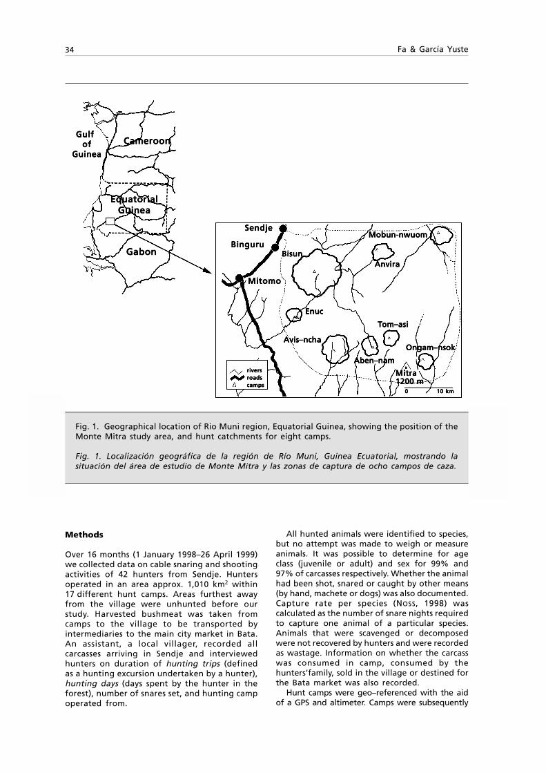
34 Fa & García Yuste
Methods
Over 16 months (1 January 1998–26 April 1999)we collected data on cable snaring and shootingactivities of 42 hunters from Sendje. Huntersoperated in an area approx. 1,010 km2 within17 different hunt camps. Areas furthest awayfrom the village were unhunted before ourstudy. Harvested bushmeat was taken fromcamps to the village to be transported byintermediaries to the main city market in Bata.An assistant, a local villager, recorded allcarcasses arriving in Sendje and interviewedhunters on duration of hunting trips (definedas a hunting excursion undertaken by a hunter),hunting days (days spent by the hunter in theforest), number of snares set, and hunting campoperated from.
All hunted animals were identified to species,but no attempt was made to weigh or measureanimals. It was possible to determine for ageclass (juvenile or adult) and sex for 99% and97% of carcasses respectively. Whether the animalhad been shot, snared or caught by other means(by hand, machete or dogs) was also documented.Capture rate per species (NOSS, 1998) wascalculated as the number of snare nights requiredto capture one animal of a particular species.Animals that were scavenged or decomposedwere not recovered by hunters and were recordedas wastage. Information on whether the carcasswas consumed in camp, consumed by thehunters’family, sold in the village or destined forthe Bata market was also recorded.
Hunt camps were geo–referenced with the aidof a GPS and altimeter. Camps were subsequently
Fig. 1. Geographical location of Rio Muni region, Equatorial Guinea, showing the position of theMonte Mitra study area, and hunt catchments for eight camps.
Fig. 1. Localización geográfica de la región de Río Muni, Guinea Ecuatorial, mostrando lasituación del área de estudio de Monte Mitra y las zonas de captura de ocho campos de caza.
Mobun-nwuomMobun-nwuomMobun-nwuomMobun-nwuomMobun-nwuom
AnviraAnviraAnviraAnviraAnviraBisunBisunBisunBisunBisun
EnucEnucEnucEnucEnuc
Avis–nchaAvis–nchaAvis–nchaAvis–nchaAvis–ncha
TTTTTom–asiom–asiom–asiom–asiom–asi
Ongam–nsokOngam–nsokOngam–nsokOngam–nsokOngam–nsok
Aben–namAben–namAben–namAben–namAben–nam
00000 10 km 10 km 10 km 10 km 10 km
MitraMitraMitraMitraMitra1200 m1200 m1200 m1200 m1200 m
riversriversriversriversriversroadsroadsroadsroadsroadscampscampscampscampscamps
MitomoMitomoMitomoMitomoMitomo
BinguruBinguruBinguruBinguruBinguru
SendjeSendjeSendjeSendjeSendje
CameroonCameroonCameroonCameroonCameroon
GabonGabonGabonGabonGabon
GulfGulfGulfGulfGulf of of of of of
Guinea Guinea Guinea Guinea Guinea
EquatorialEquatorialEquatorialEquatorialEquatorialGuineaGuineaGuineaGuineaGuinea

Animal Biodiversity and Conservation 24.1 (2001) 35
mapped onto a 1/100,000 land use map from theCUREF Project ("Conservación y Utilización Racionalde los Ecosistemas Forestales de Guinea Ecuatorial",http://www.internetafrica.com/curef/) based inBata. CUREF maps are based on radar, Spot XS andLandsat TM (1988–1995) images. Hunt catchments,defined as the area (in km2) operated by huntersduring the study, were estimated for only eightcamps (Aben–nam, Anvira, Avis–ncha, Bisun,Mobun–nwuom, Enuc, Ongam–nsok, Tom–asi). Thiswas undertaken by accompanying hunters forperiods of 2 to 20 hunting days and geo-referencingthe limits of their hunting territories (fig. 1).
Species names follow KINGDON (1997). Biomassextracted per species was calculated by multiplyingthe recorded number of carcasses of a species bythe mass of an "average" individual. Body masseswere taken from FA & PURVIS (1997) for adults,and halved for juveniles. By using productivityand population density data in FA et al. (1995) forthe same region, it was possible to evaluatesustainability of hunting for 14 mammal species(2 rodents, 6 ungulates, 5 primates, 1 pangolin)for the estimated hunt catchments. Harvest rateswere calculated by FA et al. (1995) using themethod of ROBINSON & REDFORD (1991).
Statistical analyses were carried out using S–plus (VENABLES & RIPLEY, 1999). All means arereported with one standard deviation (±1 SD).
Results
Prey Species
During the study period, hunters caught3,053 individuals of 58 species (43 mammals,8 birds, 6 reptiles, 1 snail) or 15,169.1kg. Mammalsaccounted for 79% of total captures, reptiles16%, birds 5% and snails 0.03%. By weight, 90.0%of the hunted biomass consisted of mammals,9.2% reptiles, 0.86% birds and 0.03% of snails.
Over 30% of captures were made up ofungulates (884 carcasses, 12 species), followedby rodents (27%, 826 carcasses, 7 species),reptiles (16%, 490 carcasses, 6 species) andprimates (11%, 329 carcasses, 11 species).Pangolins (2 species) were represented by224 carcasses (7%), birds by 142 (5%, 8 species),carnivores by 112 (10 species, 4%), andTubulidentates by one animal of a single species.Nine species (2 species each of rodents,ungulates, and primates, and one species ofreptile, bird and pangolin) were represented by>100 captures, but 33 species (56.89%) had lessthan 10 carcasses each. The most–capturedspecies was the blue duiker, Cephalophusmonticola, which represented 21.6% (658carcasses) of all captures and 15.3% by weight.The brush–tailed porcupine, Atherurus africanus
Fig. 2. Relationship between the body mass (kg) of the hunted bushmeat species, the number ofanimals captured and the total biomass (kg) of each species extracted.
Fig. 2. Relación entre la masa corporal (kg) de las especies de carne de selva cazadas, el númerode animales capturados y la biomasa total (kg) de cada especie extraída.
NumbersNumbersNumbersNumbersNumbers
BiomasBiomasBiomasBiomasBiomassssss
77777
66666
55555
44444
33333
22222
11111
00000
-1-1-1-1-1
-1-1-1-1-1 00000 11111 2 2 2 2 2 3 3 3 3 3 44444
Log body mass (kg)Log body mass (kg)Log body mass (kg)Log body mass (kg)Log body mass (kg)
L
og
. n
um
be
rs/b
iom
ass
(k
g)
L
og
. n
um
be
rs/b
iom
ass
(k
g)
L
og
. n
um
be
rs/b
iom
ass
(k
g)
L
og
. n
um
be
rs/b
iom
ass
(k
g)
L
og
. n
um
be
rs/b
iom
ass
(k
g)
y = 1.1659x + 0.9195y = 1.1659x + 0.9195y = 1.1659x + 0.9195y = 1.1659x + 0.9195y = 1.1659x + 0.9195RRRRR22222 = 0.6014 = 0.6014 = 0.6014 = 0.6014 = 0.6014
y = 1.1659x + 0.9195y = 1.1659x + 0.9195y = 1.1659x + 0.9195y = 1.1659x + 0.9195y = 1.1659x + 0.9195RRRRR22222 = 0.0296 = 0.0296 = 0.0296 = 0.0296 = 0.0296
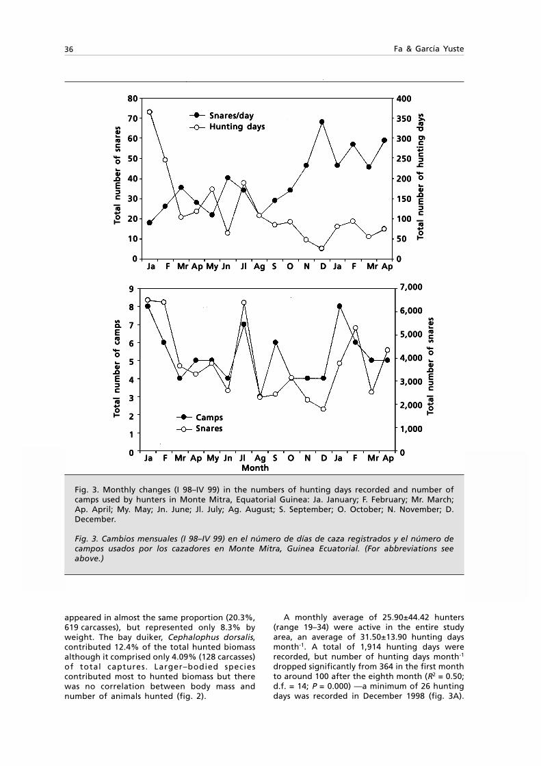
36 Fa & García Yuste
appeared in almost the same proportion (20.3%,619 carcasses), but represented only 8.3% byweight. The bay duiker, Cephalophus dorsalis,contributed 12.4% of the total hunted biomassalthough it comprised only 4.09% (128 carcasses)of total captures. Larger–bodied speciescontributed most to hunted biomass but therewas no correlation between body mass andnumber of animals hunted (fig. 2).
A monthly average of 25.90±44.42 hunters(range 19–34) were active in the entire studyarea, an average of 31.50±13.90 hunting daysmonth-1. A total of 1,914 hunting days wererecorded, but number of hunting days month-1
dropped significantly from 364 in the first monthto around 100 after the eighth month (R2 = 0.50;d.f. = 14; P = 0.000) —a minimum of 26 huntingdays was recorded in December 1998 (fig. 3A).
Fig. 3. Monthly changes (I 98–IV 99) in the numbers of hunting days recorded and number ofcamps used by hunters in Monte Mitra, Equatorial Guinea: Ja. January; F. February; Mr. March;Ap. April; My. May; Jn. June; Jl. July; Ag. August; S. September; O. October; N. November; D.December.
Fig. 3. Cambios mensuales (I 98–IV 99) en el número de días de caza registrados y el número decampos usados por los cazadores en Monte Mitra, Guinea Ecuatorial. (For abbreviations seeabove.)
Snares/daySnares/daySnares/daySnares/daySnares/dayHunting daysHunting daysHunting daysHunting daysHunting days
8080808080
7070707070
6060606060
5050505050
4040404040
3030303030
2020202020
1010101010
00000
TTTT T ota
l n
um
be
r o
f sn
are
so
tal
nu
mb
er
of
sna
res
ota
l n
um
be
r o
f sn
are
so
tal
nu
mb
er
of
sna
res
ota
l n
um
be
r o
f sn
are
sTTTT T o
tal
nu
mb
er
of
cam
ps
ota
l n
um
be
r o
f ca
mp
so
tal
nu
mb
er
of
cam
ps
ota
l n
um
be
r o
f ca
mp
so
tal
nu
mb
er
of
cam
ps
99999
88888
77777
66666
55555
44444
33333
22222
11111
00000
Ja F Mr Ja F Mr Ja F Mr Ja F Mr Ja F Mr ApApApApAp My Jn Jl Ag S O N D Ja F Mr ApMy Jn Jl Ag S O N D Ja F Mr ApMy Jn Jl Ag S O N D Ja F Mr ApMy Jn Jl Ag S O N D Ja F Mr ApMy Jn Jl Ag S O N D Ja F Mr Ap
Ja F MrJa F MrJa F MrJa F MrJa F Mr ApApApApAp MyMyMyMyMy Jn JlJn JlJn JlJn JlJn Jl Ag S O N D Ja F Mr ApAg S O N D Ja F Mr ApAg S O N D Ja F Mr ApAg S O N D Ja F Mr ApAg S O N D Ja F Mr Ap Month Month Month Month Month
400400400400400
350350350350350
300300300300300
250250250250250
200200200200200
150150150150150
100100100100100
5050505050
00000
TTTT T ota
l n
um
be
r o
f h
un
tin
g d
ays
ota
l n
um
be
r o
f h
un
tin
g d
ays
ota
l n
um
be
r o
f h
un
tin
g d
ays
ota
l n
um
be
r o
f h
un
tin
g d
ays
ota
l n
um
be
r o
f h
un
tin
g d
ays
TTTT T ota
l n
um
be
r o
f sn
are
so
tal
nu
mb
er
of
sna
res
ota
l n
um
be
r o
f sn
are
so
tal
nu
mb
er
of
sna
res
ota
l n
um
be
r o
f sn
are
s
CampsCampsCampsCampsCampsSnareSnareSnareSnareSnaresssss
7,0007,0007,0007,0007,000
6,0006,0006,0006,0006,000
5,0005,0005,0005,0005,000
4,0004,0004,0004,0004,000
3,0003,0003,0003,0003,000
2,0002,0002,0002,0002,000
1,0001,0001,0001,0001,000
00000
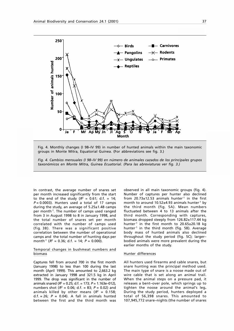
Animal Biodiversity and Conservation 24.1 (2001) 37
In contrast, the average number of snares setper month increased significantly from the startto the end of the study (R2 = 0.61; d.f. = 14;P = 0.0003). Hunters used a total of 17 campsduring the study, an average of 5.25±1.48 campsper month-1. The number of camps used rangedfrom 3 in August 1998 to 8 in January 1998, andthe total number of snares set per monthcorrelated with the number of camps used(fig. 3B). There was a significant positivecorrelation between the number of operationalcamps and the total number of hunting days permonth-1 (R2 = 0.36; d.f. = 14; P = 0.000).
Temporal changes in bushmeat numbers andbiomass
Captures fell from around 700 in the first month(January 1998) to less than 100 during the lastmonth (April 1999). This amounted to 2,663.2 kgextracted in January 1998 and 321.5 kg in April1999. The drop was significant in the number ofanimals snared (R2 = 0.25; d.f. = 173; P = 1.163e–012),numbers shot (R2 = 0.06; d.f. = 83; P = 0.02) andanimals killed by other means (R2 = 0.158;d.f. = 26; P = 0.04). A fall in animals huntedbetween the first and the third month was
observed in all main taxonomic groups (fig. 4).Number of captures per hunter also declinedfrom 20.73±12.53 animals hunter-1 in the firstmonth to around 10.52±4.93 animals hunter-1 bythe third month (fig. 5A). Mean numbersfluctuated between 4 to 13 animals after thethird month. Corresponding with captures,biomass dropped steeply from 126.82±117.44 kghunter-1 in the first month to 20.65±20.18 kghunter-1 in the third month (fig. 5B). Averagebody mass of hunted animals also declinedthroughout the study period (fig. 5C); larger–bodied animals were more prevalent during theearlier months of the study.
Hunter differences
All hunters used firearms and cable snares, butsnare hunting was the principal method used.The main type of snare is a noose made out ofwire cable that is set along an animal trail.When the animal steps on a pressure pad, itreleases a bent–over pole, which springs up totighten the noose around the animal’s leg.....During the study period, hunters deployed atotal of 56,398 snares. This amounted to107,945,772 snare–nights (the number of snares
Fig. 4. Monthly changes (I 98–IV 99) in number of hunted animals within the main taxonomicgroups in Monte Mitra, Equatorial Guinea. (For abbreviations see fig. 3.)
Fig. 4. Cambios mensuales (I 98–IV 99) en número de animales cazados de los principales grupostaxonómicos en Monte Mitra, Guinea Ecuatorial. (Para las abreviaturas ver fig. 3.)
Ja F Mr Ja F Mr Ja F Mr Ja F Mr Ja F Mr Ap Ap Ap Ap Ap My Jn Jl Ag S O N D Ja F Mr ApMy Jn Jl Ag S O N D Ja F Mr ApMy Jn Jl Ag S O N D Ja F Mr ApMy Jn Jl Ag S O N D Ja F Mr ApMy Jn Jl Ag S O N D Ja F Mr Ap Month Month Month Month Month
250250250250250
200200200200200
150150150150150
100100100100100
5050505050
00000
BirdsBirdsBirdsBirdsBirds
PangolinsPangolinsPangolinsPangolinsPangolins
UngulatesUngulatesUngulatesUngulatesUngulates
ReptilesReptilesReptilesReptilesReptiles
CarnivoresCarnivoresCarnivoresCarnivoresCarnivores
RodentsRodentsRodentsRodentsRodents
PrimatesPrimatesPrimatesPrimatesPrimates
Nu
mb
er
of
an
ima
ls h
un
ted
Nu
mb
er
of
an
ima
ls h
un
ted
Nu
mb
er
of
an
ima
ls h
un
ted
Nu
mb
er
of
an
ima
ls h
un
ted
Nu
mb
er
of
an
ima
ls h
un
ted
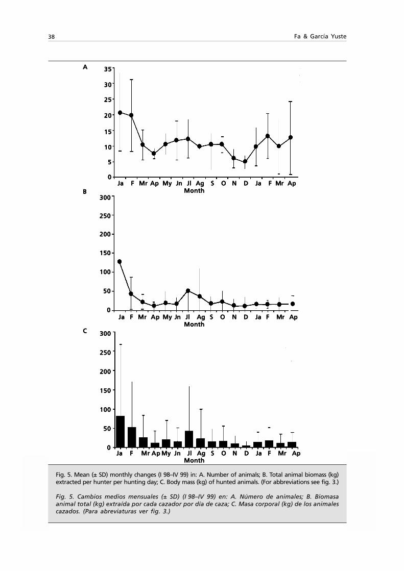
38 Fa & García Yuste
Fig. 5. Mean (± SD) monthly changes (I 98–IV 99) in: A. Number of animals; B. Total animal biomass (kg)extracted per hunter per hunting day; C. Body mass (kg) of hunted animals. (For abbreviations see fig. 3.)
Fig. 5. Cambios medios mensuales (± SD) (I 98–IV 99) en: A. Número de animales; B. Biomasaanimal total (kg) extraída por cada cazador por día de caza; C. Masa corporal (kg) de los animalescazados. (Para abreviaturas ver fig. 3.)
Ja Ja Ja Ja Ja F F F F F MrMrMrMrMr ApApApApAp MyMyMyMyMy JnJnJnJnJn JlJlJlJlJl Ag Ag Ag Ag Ag S O S O S O S O S O N N N N N D Ja D Ja D Ja D Ja D Ja F MrF MrF MrF MrF Mr ApApApApAp Month Month Month Month Month
Ja Ja Ja Ja Ja F F F F F Mr Ap Mr Ap Mr Ap Mr Ap Mr Ap MyMyMyMyMy Jn JlJn JlJn JlJn JlJn Jl Ag Ag Ag Ag Ag S O S O S O S O S O N N N N N D D D D D Ja F Ja F Ja F Ja F Ja F Mr Mr Mr Mr Mr ApApApApAp Month Month Month Month Month
JaJaJaJaJa F F F F F Mr Mr Mr Mr Mr ApApApApAp My My My My My Jn Jl Jn Jl Jn Jl Jn Jl Jn Jl Ag S O N Ag S O N Ag S O N Ag S O N Ag S O N D D D D D Ja F Mr ApJa F Mr ApJa F Mr ApJa F Mr ApJa F Mr Ap Month Month Month Month Month
AAAAA
BBBBB
CCCCC
3535353535
3030303030
2525252525
2020202020
1515151515
1010101010
55555
00000
300300300300300
250250250250250
200200200200200
150150150150150
100100100100100
5050505050
00000
300300300300300
250250250250250
200200200200200
150150150150150
100100100100100
5050505050
00000

Animal Biodiversity and Conservation 24.1 (2001) 39
times the number of nights set), an average of1,927,603 snare–nights per hunter. An averageof 112.06±57.34 snares (136,358.31±118,441.48snare nights ranging from 28,303 snare nights inJune 1998 to 408,192 snare nights in July 1998)were operational every month throughout thestudy area, with no significant monthly variationbeing detected. However, number of snares setin each camp differed significantly, from50.0±70.7 snares hunting trip-1 in Sendje to222.4±106.9 snares hunting trip-1 in Aben–nam(Goodness of fit test, R2 = 286.35; d.f. = 15;P = 1.7e–51). Per camp, the number of snares setwas not correlated with the number of huntersoperating in the area (R2 = 0.002; d.f. = 40; NS)or with the size of the hunt catchment area(R2 = 0.0002; d.f. = 6; NS).
A total of 563 hunting trips was recorded forthe 42 hunters in the area. Each hunter undertook13.73±13.96 (range 1–52) hunting trips duringthe study period, and spent an average of46.27±54.49 (range 1–233 days) total huntingdays (table 1). Hunting trips lasted 3.81±3.21days per hunter (range 1.00±0.00–9.43±4.34 days)during which 1,484.16±1723.92 snares wereoperated per hunter (range 80–5,459 snares).The hunting trip duration did not differsignificantly among hunters (R2 = 12.11; d.f. = 40;P = 0.74). However, the number of snaresoperated per hunter varied significantly(R2 = 80025.98; d.f. = 40; P = 0.000).
Number of animals hunted and biomassextracted per hunter were positively correlatedwith total number of hunting days (fig. 6). Biomassextracted and captures per hunter were alsopositively correlated with number of snares set(R2 = 0.48; d.f. = 40; P = 0.000). However, the totalnumber of camps used was not correlated withnumber of hunting trips completed by each hunter.
Hunters extracted 66.29±66.51 animals or270.87±219.35 kg of animal biomass hunter-1
during the study period or a mean of 50 animalsor 203.18 kg hunter-1 annum-1. Number ofanimals hunted (R2= 2736.22; d.f. = 40; P = 0.000)and biomass extracted (R2= 7282.53; d.f. = 40;P = 0.000) varied significantly among hunters.The most productive hunter was Hunter 8, whocaptured a total of 276 animals on 52 huntingtrips whilst Hunter 42, the least prolific, caught asingle animal on any one hunting trip. Mostanimals were caught by snares (60.83±67.23animals hunter-1), and significantly fewer animalswere shot (5.45±10.27 animals hunter-1). Numberof animals extracted per hunting day by eachhunter averaged 0.83±1.72 for the study period.The lowest monthly extraction figure was forApril 1998 (0.53±0.41 animals hunter-1 huntingday-1) whilst the highest (1.78±1.82 animalshunter-1 hunting day-1) was in January 1999.There was no significant inter–monthlydifference in number of animals extracted byhunters (R2= 3.74; d.f. = 14; P = 0.999).
Hunters used from one to six camps, 2.29±1.50
camps per hunter (median 2 camps). Most(n = 19 hunters; 45.24% of all hunters) usedonly one camp, eight (19.05%) used two camps,14 (33.33%) from three to five camps, but asingle hunter (2.38%) operated in six differentcamps. Only one hunter used Esua–asas andEto–mbeng, but a maximum of 20 huntersentered Bisun (table 2). Number of snares setper trip in each camp varied from 50.0±57.74 inSendje to 222.35±106.85 in Aben–nam. Anaverage of 112.96±54.25 snares per huntcatchment was set during each hunting trip.
Camp differences
For the camps surveyed, regular hunt catchmentswere an average of 28.3±±±±±8.9 km from the village,,,,,ranging from 11.7 km (Bisun) to 41.7 km (Ongam–nsok) (table 2). Hunt catchments varied signifi-cantly in size from 6.2 km2 in Ongam–nsok to314.2 km2 in Bisun, with the larger areas beingfound closer to the village (R2 = 0.63; d.f. = 6; P =0.019). The size of the hunted areas was correlatedwith the number of hunters operating withinthem (R2 = 0.59; d.f. = 6; P = 0.020).
Per camp, annual harvests varied from5 animals (4.77 kg) in Esua–asas to 764 animals(4,413.53 kg) in Bisun. Biomass extracted perhunter differed significantly between camps(R2 = 957.5; d.f. = 15; P = 1.4e–193). Biomassextracted per camp per hunting day also variedsignificantly (R2 = 29.7; d.f. = 15; P = 0.013). Forthose camps for which hunt catchment area wasmeasured, number of animals and biomassextracted per km2 differed significantly betweencamps (table 3). Ongam–nsok was by far the mostproductive with 224.47 kg of bushmeat km-2,whereas Bisun, which was also the most huntedcamp, produced 14.05 kg bushmeat km-2
(R2 = 667.5; d.f. = 15; P = 1.6e132).
Proportion of species sold and consumed
Although some meat is for home consumption(22.87%), the largest proportion of animalshunted (67.77%) was either sold in Sendje(34.05%) or in the Bata market (33.72%).Bushmeat consumed by the hunters’families was16.26%, and hunters themselves would consume6.61% in forest. Only 9.35% of the total numberof recorded animals was unsuitable forconsumption. The number of animals sold(R2 = 0.02; d.f. = 56; NS) or consumed (R2 = 0.02;d.f. = 56; NS) was not correlated with the numberof carcasses per species hunted. Similarly, biomasswas not correlated with proportion sold(R2 = 0.02; d.f. = 56; NS) or consumed (R2 = 0.03;d.f. = 56; NS). Per hunter, an average of39.02±26.98% of the animals hunted were soldto the Bata market.
For the subsample of species with >100carcasses (7 mammals, 2 reptiles, 1 bird), theproportion of animals sold to the Bata market
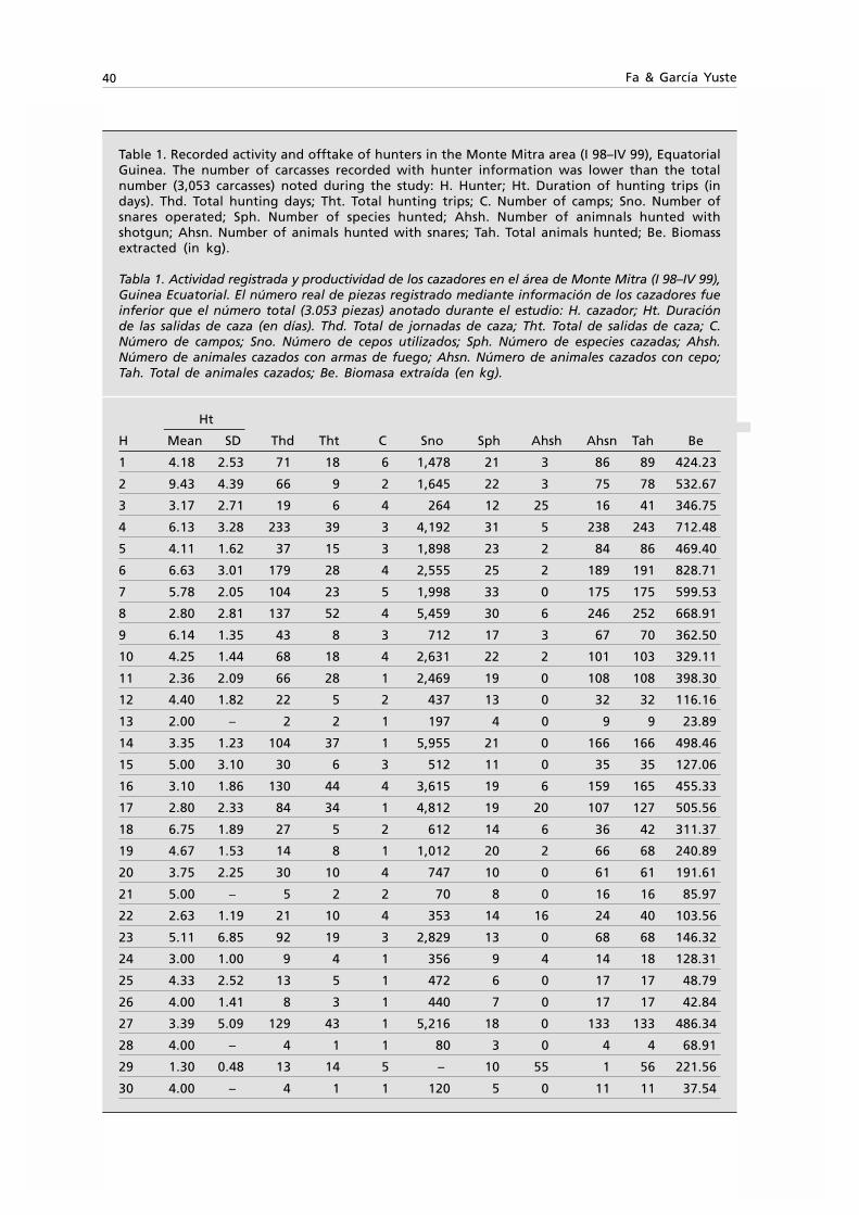
40 Fa & García Yuste
Table 1. Recorded activity and offtake of hunters in the Monte Mitra area (I 98–IV 99), EquatorialGuinea. The number of carcasses recorded with hunter information was lower than the totalnumber (3,053 carcasses) noted during the study: H. Hunter; Ht. Duration of hunting trips (indays). Thd. Total hunting days; Tht. Total hunting trips; C. Number of camps; Sno. Number ofsnares operated; Sph. Number of species hunted; Ahsh. Number of animnals hunted withshotgun; Ahsn. Number of animals hunted with snares; Tah. Total animals hunted; Be. Biomassextracted (in kg).
Tabla 1. Actividad registrada y productividad de los cazadores en el área de Monte Mitra (I 98–IV 99),Guinea Ecuatorial. El número real de piezas registrado mediante información de los cazadores fueinferior que el número total (3.053 piezas) anotado durante el estudio: H. cazador; Ht. Duraciónde las salidas de caza (en días). Thd. Total de jornadas de caza; Tht. Total de salidas de caza; C.Número de campos; Sno. Número de cepos utilizados; Sph. Número de especies cazadas; Ahsh.Número de animales cazados con armas de fuego; Ahsn. Número de animales cazados con cepo;Tah. Total de animales cazados; Be. Biomasa extraída (en kg).
Ht
H Mean SD Thd Tht C Sno Sph Ahsh Ahsn Tah Be
1 4.18 2.53 71 18 6 1,478 21 3 86 89 424.23
2 9.43 4.39 66 9 2 1,645 22 3 75 78 532.67
3 3.17 2.71 19 6 4 264 12 25 16 41 346.75
4 6.13 3.28 233 39 3 4,192 31 5 238 243 712.48
5 4.11 1.62 37 15 3 1,898 23 2 84 86 469.40
6 6.63 3.01 179 28 4 2,555 25 2 189 191 828.71
7 5.78 2.05 104 23 5 1,998 33 0 175 175 599.53
8 2.80 2.81 137 52 4 5,459 30 6 246 252 668.91
9 6.14 1.35 43 8 3 712 17 3 67 70 362.50
10 4.25 1.44 68 18 4 2,631 22 2 101 103 329.11
11 2.36 2.09 66 28 1 2,469 19 0 108 108 398.30
12 4.40 1.82 22 5 2 437 13 0 32 32 116.16
13 2.00 – 2 2 1 197 4 0 9 9 23.89
14 3.35 1.23 104 37 1 5,955 21 0 166 166 498.46
15 5.00 3.10 30 6 3 512 11 0 35 35 127.06
16 3.10 1.86 130 44 4 3,615 19 6 159 165 455.33
17 2.80 2.33 84 34 1 4,812 19 20 107 127 505.56
18 6.75 1.89 27 5 2 612 14 6 36 42 311.37
19 4.67 1.53 14 8 1 1,012 20 2 66 68 240.89
20 3.75 2.25 30 10 4 747 10 0 61 61 191.61
21 5.00 – 5 2 2 70 8 0 16 16 85.97
22 2.63 1.19 21 10 4 353 14 16 24 40 103.56
23 5.11 6.85 92 19 3 2,829 13 0 68 68 146.32
24 3.00 1.00 9 4 1 356 9 4 14 18 128.31
25 4.33 2.52 13 5 1 472 6 0 17 17 48.79
26 4.00 1.41 8 3 1 440 7 0 17 17 42.84
27 3.39 5.09 129 43 1 5,216 18 0 133 133 486.34
28 4.00 – 4 1 1 80 3 0 4 4 68.91
29 1.30 0.48 13 14 5 – 10 55 1 56 221.56
30 4.00 – 4 1 1 120 5 0 11 11 37.54
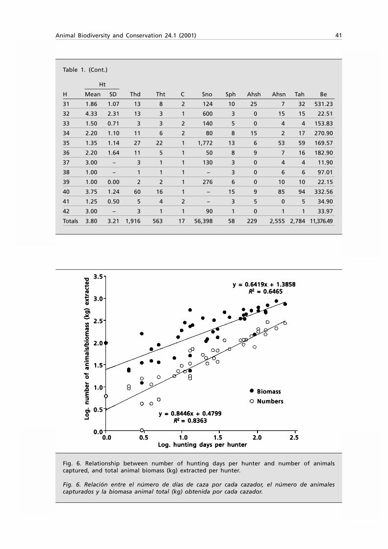
Animal Biodiversity and Conservation 24.1 (2001) 41
Fig. 6. Relationship between number of hunting days per hunter and number of animalscaptured, and total animal biomass (kg) extracted per hunter.
Fig. 6. Relación entre el número de días de caza por cada cazador, el número de animalescapturados y la biomasa animal total (kg) obtenida por cada cazador.
31 1.86 1.07 13 8 2 124 10 25 7 32 531.23
32 4.33 2.31 13 3 1 600 3 0 15 15 22.51
33 1.50 0.71 3 3 2 140 5 0 4 4 153.83
34 2.20 1.10 11 6 2 80 8 15 2 17 270.90
35 1.35 1.14 27 22 1 1,772 13 6 53 59 169.57
36 2.20 1.64 11 5 1 50 8 9 7 16 182.90
37 3.00 – 3 1 1 130 3 0 4 4 11.90
38 1.00 – 1 1 1 – 3 0 6 6 97.01
39 1.00 0.00 2 2 1 276 6 0 10 10 22.15
40 3.75 1.24 60 16 1 – 15 9 85 94 332.56
41 1.25 0.50 5 4 2 – 3 5 0 5 34.90
42 3.00 – 3 1 1 90 1 0 1 1 33.97
Totals 3.80 3.21 1,916 563 17 56,398 58 229 2,555 2,784 11,376.49
Table 1. (Cont.)
3.53.53.53.53.5
3.03.03.03.03.0
2.52.52.52.52.5
2.02.02.02.02.0
1.51.51.51.51.5
1.01.01.01.01.0
0.50.50.50.50.5
0.00.00.00.00.0
Log
. n
um
be
r o
f a
nim
als
/bio
ma
ss (
kg
) e
xtra
cte
dLo
g.
nu
mb
er
of
an
ima
ls/b
iom
ass
(k
g)
ext
ract
ed
Log
. n
um
be
r o
f a
nim
als
/bio
ma
ss (
kg
) e
xtra
cte
dLo
g.
nu
mb
er
of
an
ima
ls/b
iom
ass
(k
g)
ext
ract
ed
Log
. n
um
be
r o
f a
nim
als
/bio
ma
ss (
kg
) e
xtra
cte
d
0.0 0.0 0.0 0.0 0.0 0.5 0.5 0.5 0.5 0.5 1.0 1.0 1.0 1.0 1.0 1.5 1.5 1.5 1.5 1.5 2.0 2.0 2.0 2.0 2.0 2.5 2.5 2.5 2.5 2.5Log. hunting days per hunterLog. hunting days per hunterLog. hunting days per hunterLog. hunting days per hunterLog. hunting days per hunter
y = 0.8446x + 0.4799y = 0.8446x + 0.4799y = 0.8446x + 0.4799y = 0.8446x + 0.4799y = 0.8446x + 0.4799RRRRR2 2 2 2 2 = 0.8363= 0.8363= 0.8363= 0.8363= 0.8363
BiomassBiomassBiomassBiomassBiomass
NumbersNumbersNumbersNumbersNumbers
y = 0.6419x + 1.3858y = 0.6419x + 1.3858y = 0.6419x + 1.3858y = 0.6419x + 1.3858y = 0.6419x + 1.3858 R R R R R22222 = 0.6465 = 0.6465 = 0.6465 = 0.6465 = 0.6465
Ht
H Mean SD Thd Tht C Sno Sph Ahsh Ahsn Tah Be
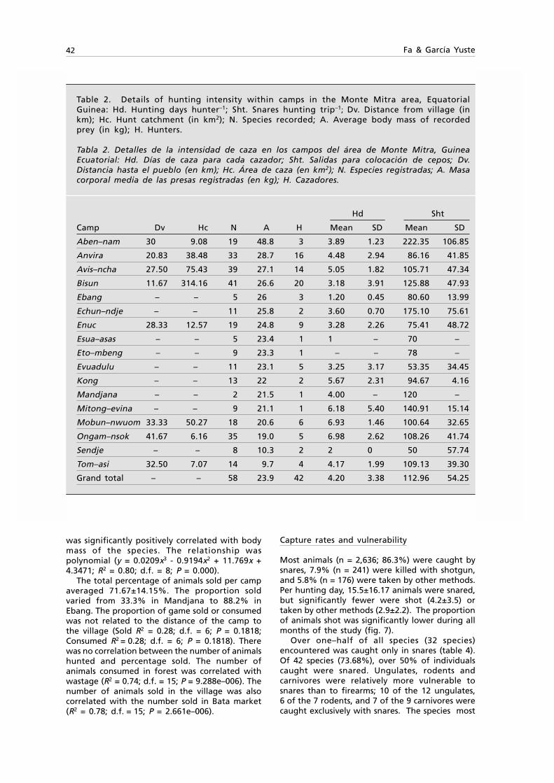
42 Fa & García Yuste
Table 2. Details of hunting intensity within camps in the Monte Mitra area, EquatorialGuinea: Hd. Hunting days hunter–1; Sht. Snares hunting trip–1; Dv. Distance from village (inkm); Hc. Hunt catchment (in km2); N. Species recorded; A. Average body mass of recordedprey (in kg); H. Hunters.
Tabla 2. Detalles de la intensidad de caza en los campos del área de Monte Mitra, GuineaEcuatorial: Hd. Días de caza para cada cazador; Sht. Salidas para colocación de cepos; Dv.Distancia hasta el pueblo (en km); Hc. Área de caza (en km2); N. Especies registradas; A. Masacorporal media de las presas registradas (en kg); H. Cazadores.
Hd Sht
Camp Dv Hc N A H Mean SD Mean SD
Aben–nam 30 9.08 19 48.8 3 3.89 1.23 222.35 106.85
Anvira 20.83 38.48 33 28.7 16 4.48 2.94 86.16 41.85
Avis–ncha 27.50 75.43 39 27.1 14 5.05 1.82 105.71 47.34
Bisun 11.67 314.16 41 26.6 20 3.18 3.91 125.88 47.93
Ebang – – 5 26 3 1.20 0.45 80.60 13.99
Echun–ndje – – 11 25.8 2 3.60 0.70 175.10 75.61
Enuc 28.33 12.57 19 24.8 9 3.28 2.26 75.41 48.72
Esua–asas – – 5 23.4 1 1 – 70 –
Eto–mbeng – – 9 23.3 1 – – 78 –
Evuadulu – – 11 23.1 5 3.25 3.17 53.35 34.45
Kong – – 13 22 2 5.67 2.31 94.67 4.16
Mandjana – – 2 21.5 1 4.00 – 120 –
Mitong–evina – – 9 21.1 1 6.18 5.40 140.91 15.14
Mobun–nwuom 33.33 50.27 18 20.6 6 6.93 1.46 100.64 32.65
Ongam–nsok 41.67 6.16 35 19.0 5 6.98 2.62 108.26 41.74
Sendje – – 8 10.3 2 2 0 50 57.74
Tom–asi 32.50 7.07 14 9.7 4 4.17 1.99 109.13 39.30
Grand total – – 58 23.9 42 4.20 3.38 112.96 54.25
was significantly positively correlated with bodymass of the species. The relationship waspolynomial (y = 0.0209x3 - 0.9194x2 + 11.769x +4.3471; R2 = 0.80; d.f. = 8; P = 0.000).
The total percentage of animals sold per campaveraged 71.67±14.15%. The proportion soldvaried from 33.3% in Mandjana to 88.2% inEbang. The proportion of game sold or consumedwas not related to the distance of the camp tothe village (Sold R2 = 0.28; d.f. = 6; P = 0.1818;Consumed R2 = 0.28; d.f. = 6; P = 0.1818). Therewas no correlation between the number of animalshunted and percentage sold. The number ofanimals consumed in forest was correlated withwastage (R2 = 0.74; d.f. = 15; P = 9.288e–006). Thenumber of animals sold in the village was alsocorrelated with the number sold in Bata market(R2 = 0.78; d.f. = 15; P = 2.661e–006).
Capture rates and vulnerability
Most animals (n = 2,636; 86.3%) were caught bysnares, 7.9% (n = 241) were killed with shotgun,and 5.8% (n = 176) were taken by other methods.Per hunting day, 15.5±16.17 animals were snared,but significantly fewer were shot (4.2±3.5) ortaken by other methods (2.9±2.2). The proportionof animals shot was significantly lower during allmonths of the study (fig. 7).
Over one–half of all species (32 species)encountered was caught only in snares (table 4).Of 42 species (73.68%), over 50% of individualscaught were snared. Ungulates, rodents andcarnivores were relatively more vulnerable tosnares than to firearms; 10 of the 12 ungulates,6 of the 7 rodents, and 7 of the 9 carnivores werecaught exclusively with snares. The species most

Animal Biodiversity and Conservation 24.1 (2001) 43
Table 3. Captures, wastage and hunting method for bushmeat species in Monte Mitra, EquatorialGuinea: Hm. Hunting method (%); C. Captures; Sn. Snares; Sh. Shotgun.
Tabla 3. Capturas, piezas desaprovechadas y métodos de caza para carne de selva en MonteMitra, Guinea Ecuatorial: Hm. Método de caza (%); C. Capturas; Sn. Cepos; Sh. Armas de fuego.
Groups Capture rate Wastage Hm (%)
Species Mean SD C N % Sn Sh Other
Snails
Achatina spp. – – 1 0 0 0 0 100
Reptiles
Bitis gabonica 2,991.25 2,292.82 6 0 0 100 0 0
Chamaleo cristatus 4,333 2,907.62 3 0 0 33.3 0 66.7
Kynixis erosa 211.92 219.63 337 0 0 60.2 0 39.8
Osteolaemus tetraspis 1,095.93 1,367.91 45 3 6.7 50 50 0
Python sebae 7,272.83 3,845.01 4 0 0 100 0 0
Varanus niloticus 1,028.78 994.66 92 3 3.3 95.7 0 4.3
Group total 2,822.29 2,650.63 487 6 1.2 66.6 4.6 28.8
Birds
Ceratogymna atrata 2,209.67 3,619.46 3 0 0 33.3 66.7 0
Francolinus lathanmi 3,562.75 2,026.69 9 2 22.2 100 0 0
Gypohierax angolensis – – 1 0 0 0 100 0
Haliaetus vocifer – – 1 0 0 0 100 0
Numida meleagris 908.47 1,117.57 118 17 14.4 97.5 2.5 0
Obom (unidentified bird) 29,975 – 1 0 0 100 0 0
Psittacus erithacus 551.93 714.55 8 0 0 100 0 0
Stephanoaetus coronatus 29,975 – 1 0 0 100 0 0
Group total 11,197.14 14,583.91 143 19 13.3 94.4 4.9 0.7
Carnivores
Bdeogale nigripes 3,375.67 2,738.74 3 0 0 100 0 0
Civicttis civetta 3,667.58 6,331.87 26 4 15.4 100 0 0
Crossarchus obscurus 5,452.19 6,419.79 10 1 10 100 0 0
Felis aurata 4,744.46 6,009.13 11 1 9.1 100 0 0
Genetta tigrina/servalina 1,822.29 790.6 26 2 7.7 100 0 0
Herpestes sanguinea 7,394.83 6,644.5 7 1 14.3 100 0 0
Lutra maculicolis 5,837.50 779.94 2 0 0 100 0 0
Panthera pardus 9,091 8,338.91 4 1 25 66.7 33.3 0
Poiana richardsoni 2,555.46 2,438.79 23 6 26.1 90.9 9.1 0
Group total 4,882.33 2,340.02 112 16 14.3 96.9 3.1 0
Hyrax
Dendrohyrax dorsalis 4,150.44 570.72 9 1 11.1 100 0 0
Group total 4,150.44 570.72 9 1 11.1 100 0 0
Pangolins
Phataginus tricuspis 276.13 302.86 222 32 14.4 100 0 0
Smutsia gigantea – – 2 0 0 0 100 0
Group total – – 224 32 – 99.1 0.9 0
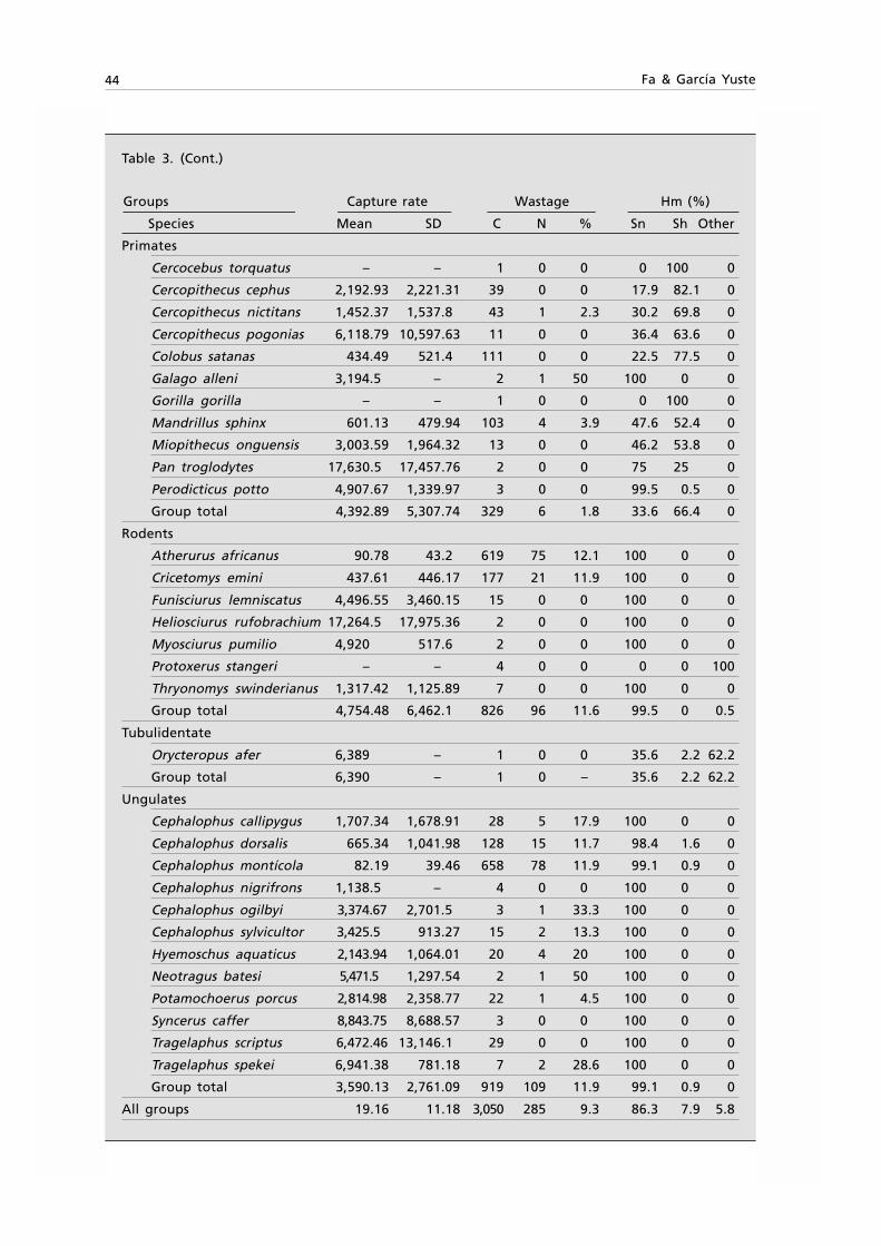
44 Fa & García Yuste
Primates
Cercocebus torquatus – – 1 0 0 0 100 0
Cercopithecus cephus 2,192.93 2,221.31 39 0 0 17.9 82.1 0
Cercopithecus nictitans 1,452.37 1,537.8 43 1 2.3 30.2 69.8 0
Cercopithecus pogonias 6,118.79 10,597.63 11 0 0 36.4 63.6 0
Colobus satanas 434.49 521.4 111 0 0 22.5 77.5 0
Galago alleni 3,194.5 – 2 1 50 100 0 0
Gorilla gorilla – – 1 0 0 0 100 0
Mandrillus sphinx 601.13 479.94 103 4 3.9 47.6 52.4 0
Miopithecus onguensis 3,003.59 1,964.32 13 0 0 46.2 53.8 0
Pan troglodytes 17,630.5 17,457.76 2 0 0 75 25 0
Perodicticus potto 4,907.67 1,339.97 3 0 0 99.5 0.5 0
Group total 4,392.89 5,307.74 329 6 1.8 33.6 66.4 0
Rodents
Atherurus africanus 90.78 43.2 619 75 12.1 100 0 0
Cricetomys emini 437.61 446.17 177 21 11.9 100 0 0
Funisciurus lemniscatus 4,496.55 3,460.15 15 0 0 100 0 0
Heliosciurus rufobrachium 17,264.5 17,975.36 2 0 0 100 0 0
Myosciurus pumilio 4,920 517.6 2 0 0 100 0 0
Protoxerus stangeri – – 4 0 0 0 0 100
Thryonomys swinderianus 1,317.42 1,125.89 7 0 0 100 0 0
Group total 4,754.48 6,462.1 826 96 11.6 99.5 0 0.5
Tubulidentate
Orycteropus afer 6,389 – 1 0 0 35.6 2.2 62.2
Group total 6,390 – 1 0 – 35.6 2.2 62.2
Ungulates
Cephalophus callipygus 1,707.34 1,678.91 28 5 17.9 100 0 0
Cephalophus dorsalis 665.34 1,041.98 128 15 11.7 98.4 1.6 0
Cephalophus montícola 82.19 39.46 658 78 11.9 99.1 0.9 0
Cephalophus nigrifrons 1,138.5 – 4 0 0 100 0 0
Cephalophus ogilbyi 3,374.67 2,701.5 3 1 33.3 100 0 0
Cephalophus sylvicultor 3,425.5 913.27 15 2 13.3 100 0 0
Hyemoschus aquaticus 2,143.94 1,064.01 20 4 20 100 0 0
Neotragus batesi 5,471.5 1,297.54 2 1 50 100 0 0
Potamochoerus porcus 2,814.98 2,358.77 22 1 4.5 100 0 0
Syncerus caffer 8,843.75 8,688.57 3 0 0 100 0 0
Tragelaphus scriptus 6,472.46 13,146.1 29 0 0 100 0 0
Tragelaphus spekei 6,941.38 781.18 7 2 28.6 100 0 0
Group total 3,590.13 2,761.09 919 109 11.9 99.1 0.9 0
All groups 19.16 11.18 3,050 285 9.3 86.3 7.9 5.8
Table 3. (Cont.)
Groups Capture rate Wastage Hm (%)
Species Mean SD C N % Sn Sh Other
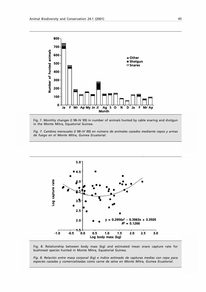
Animal Biodiversity and Conservation 24.1 (2001) 45
Fig. 8. Relationship between body mass (kg) and estimated mean snare capture rate forbushmeat species hunted in Monte Mitra, Equatorial Guinea.
Fig. 8. Relación entre masa corporal (kg) e índice estimado de capturas medias con cepo paraespecies cazadas y comercializadas como carne de selva en Monte Mitra, Guinea Ecuatorial.
Fig. 7. Monthly changes (I 98–IV 99) in number of animals hunted by cable snaring and shotgunin the Monte Mitra, Equatorial Guinea.
Fig. 7. Cambios mensuales (I 98–IV 99) en número de animales cazados mediante cepos y armasde fuego en el Monte Mitra, Guinea Ecuatorial.
OtherOtherOtherOtherOtherShotgunShotgunShotgunShotgunShotgunSnaresSnaresSnaresSnaresSnares
800800800800800
700700700700700
600600600600600
500500500500500
400400400400400
300300300300300
200200200200200
100100100100100
00000
Nu
mb
er
of
hu
nte
d a
nim
als
Nu
mb
er
of
hu
nte
d a
nim
als
Nu
mb
er
of
hu
nte
d a
nim
als
Nu
mb
er
of
hu
nte
d a
nim
als
Nu
mb
er
of
hu
nte
d a
nim
als
Ja F Mr Ja F Mr Ja F Mr Ja F Mr Ja F Mr Ap Ap Ap Ap Ap My Jn Jl Ag S O N D Ja F Mr ApMy Jn Jl Ag S O N D Ja F Mr ApMy Jn Jl Ag S O N D Ja F Mr ApMy Jn Jl Ag S O N D Ja F Mr ApMy Jn Jl Ag S O N D Ja F Mr Ap Month Month Month Month Month
5.05.05.05.05.0
4.54.54.54.54.5
4.04.04.04.04.0
3.53.53.53.53.5
3.03.03.03.03.0
2.52.52.52.52.5
2.02.02.02.02.0
1.51.51.51.51.5 -1.0 -0.5 0.0 -1.0 -0.5 0.0 -1.0 -0.5 0.0 -1.0 -0.5 0.0 -1.0 -0.5 0.0 0.5 0.5 0.5 0.5 0.5 1.0 1.5 2.0 2.5 3.0 1.0 1.5 2.0 2.5 3.0 1.0 1.5 2.0 2.5 3.0 1.0 1.5 2.0 2.5 3.0 1.0 1.5 2.0 2.5 3.0
Log body mass (kg)Log body mass (kg)Log body mass (kg)Log body mass (kg)Log body mass (kg)
Log
ca
ptu
re r
ate
Log
ca
ptu
re r
ate
Log
ca
ptu
re r
ate
Log
ca
ptu
re r
ate
Log
ca
ptu
re r
ate
y = 0.2956xy = 0.2956xy = 0.2956xy = 0.2956xy = 0.2956x22222 – 0.3963x + 3.3505 – 0.3963x + 3.3505 – 0.3963x + 3.3505 – 0.3963x + 3.3505 – 0.3963x + 3.3505RRRRR22222 = 0.1266 = 0.1266 = 0.1266 = 0.1266 = 0.1266
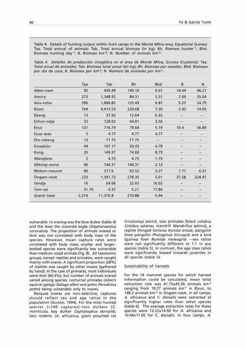
46 Fa & García Yuste
Table 4. Details of hunting output within hunt camps in the Monte Mitra area, Equatorial Guinea:Taa. Total annual of animals; Tab. Total annual biomass (in kg); Bh. Biomass hunter–1; Bhd.Biomass hunting day–1; B. Biomass km–2; N. Number of animals km–2.
Tabla 4. Detalles de producción cinegética en el área de Monte Mitra, Guinea Ecuatorial: Taa.Total anual de animales; Tab. Biomasa total anual (en kg); Bh. Biomasa por cazador; Bhd. Biomasapor día de caza; B. Biomasa por km-2; N. Número de animales por km-2.
Taa Tab Bh Bhd B N
Aben–nam 95 420.49 140.16 6.01 10.44 46.21
Anvira 273 1,348.92 84.31 5.31 7.09 35.04
Avis–ncha 396 1,868.85 133.49 6.87 5.25 24.79
Bisun 764 4,413.53 220.68 7.30 2.43 14.05
Ebang 13 37.92 12.64 6.32 – –
Echun–ndje 32 128.02 64.01 3.56 – –
Enuc 131 716.79 79.64 5.19 10.4 56.89
Esua–asas 5 4.77 4.77 4.77 – –
Eto–mbeng 13 71.75 71.75 – – –
Evuadulu 44 167.17 33.43 4.78 – –
Kong 35 149.37 74.69 8.79 – –
Mandjana 2 4.75 4.75 1.19 – –
Mitong–evina 46 144.31 144.31 2.12 – –
Mobun–nwuom 86 317.6 63.52 3.27 1.71 6.31
Ongam–nsok 233 1,391.73 278.35 5.01 37.58 224.47
Sendje 16 64.06 32.03 16.02 – –
Tom–asi 31.70 4.37 5.21 17.86 – –
Grand total 2,219 11,376.8 270.88 5.94 – –
vulnerable to snaring was the blue duiker (table 4)and the least the crowned eagle (Stephanaeotuscoronatus). The proportion of animals snared orshot was not correlated with body mass of thespecies. However, mean capture rates werecorrelated with body mass; smaller and larger–bodied species were significantly less vulnerablethan medium–sized animals (fig. 8). All taxonomicgroups, except reptiles and primates, were caughtmainly with snares. A significant proportion (28%)of reptiles was caught by other means (gatheredby hand). In the case of primates, most individualswere shot (66.4%), but number of animals snaredvaried among species; nocturnal primates (Allen’ssquirrel galago Galago alleni and potto Perodictuspotto) being vulnerable only to snares.
Because snares are non–selective, capturesshould reflect sex and age ratios in thepopulation (ALVARD, 1994). For the most huntedspecies (>100 captures)–two duikers (C.montícola, bay duiker Cephalophus dorsalis),two rodents (A. africanus, giant pouched rat
Cricetomys emini), two primates (black colobusColobus satanas, mandrill Mandrillus sphinx), areptile (hinged tortoise Kynixis erosa), pangolin(tree pangolin Phataginus tricuspis) and a bird(guinea fowl Numida meleagris) —sex ratioswere not significantly different to 1:1 in anyspecies (table 5). In contrast, the age class ratioswere significantly biased towards juveniles inall species (table 5).
Sustainability of harvests
For the 14 mammal species for which harvestinformation could be calculated, mean totalextraction rate was 41.75±45.56 animals km-2
ranging from 10.27 animals km-2 in Bisun, to148.2 animals km-2 in Ongam–nsok. In all camps,A. africanus and C. dorsalis were extracted atsignificantly higher rates than other species(table 6). The average extraction rates for thesespecies were 12.22±14.50 for A. africanus and10.44±11.05 for C. dorsalis. In four camps, A.
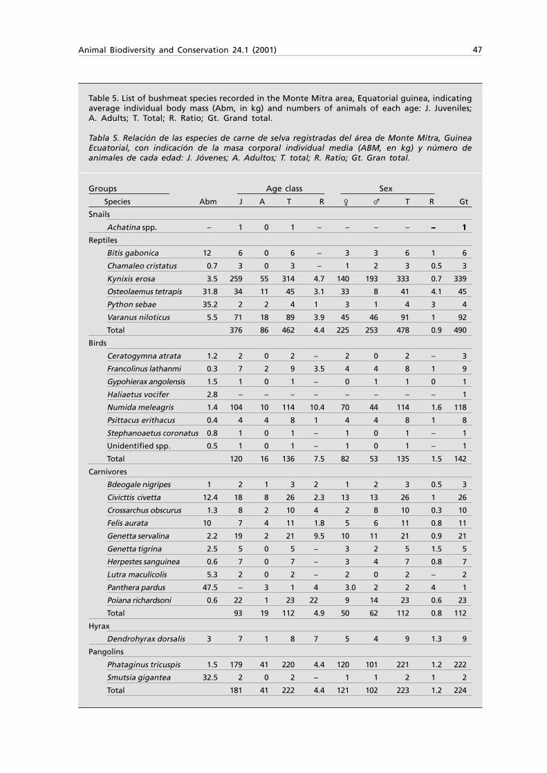
Animal Biodiversity and Conservation 24.1 (2001) 47
Table 5. List of bushmeat species recorded in the Monte Mitra area, Equatorial guinea, indicatingaverage individual body mass (Abm, in kg) and numbers of animals of each age: J. Juveniles;A. Adults; T. Total; R. Ratio; Gt. Grand total.
Tabla 5. Relación de las especies de carne de selva registradas del área de Monte Mitra, GuineaEcuatorial, con indicación de la masa corporal individual media (ABM, en kg) y número deanimales de cada edad: J. Jóvenes; A. Adultos; T. total; R. Ratio; Gt. Gran total.
Groups Age class Sex
Species Abm J A T R } { T R Gt
Snails
Achatina spp. – 1 0 1 – – – – ––––– 11111
Reptiles
Bitis gabonica 12 6 0 6 – 3 3 6 1 6
Chamaleo cristatus 0.7 3 0 3 – 1 2 3 0.5 3
Kynixis erosa 3.5 259 55 314 4.7 140 193 333 0.7 339
Osteolaemus tetrapis 31.8 34 11 45 3.1 33 8 41 4.1 45
Python sebae 35.2 2 2 4 1 3 1 4 3 4
Varanus niloticus 5.5 71 18 89 3.9 45 46 91 1 92
Total 376 86 462 4.4 225 253 478 0.9 490
Birds
Ceratogymna atrata 1.2 2 0 2 – 2 0 2 – 3
Francolinus lathanmi 0.3 7 2 9 3.5 4 4 8 1 9
Gypohierax angolensis 1.5 1 0 1 – 0 1 1 0 1
Haliaetus vocifer 2.8 – – – – – – – – 1
Numida meleagris 1.4 104 10 114 10.4 70 44 114 1.6 118
Psittacus erithacus 0.4 4 4 8 1 4 4 8 1 8
Stephanoaetus coronatus 0.8 1 0 1 – 1 0 1 – 1
Unidentified spp. 0.5 1 0 1 – 1 0 1 – 1
Total 120 16 136 7.5 82 53 135 1.5 142
Carnivores
Bdeogale nigripes 1 2 1 3 2 1 2 3 0.5 3
Civicttis civetta 12.4 18 8 26 2.3 13 13 26 1 26
Crossarchus obscurus 1.3 8 2 10 4 2 8 10 0.3 10
Felis aurata 10 7 4 11 1.8 5 6 11 0.8 11
Genetta servalina 2.2 19 2 21 9.5 10 11 21 0.9 21
Genetta tigrina 2.5 5 0 5 – 3 2 5 1.5 5
Herpestes sanguinea 0.6 7 0 7 – 3 4 7 0.8 7
Lutra maculicolis 5.3 2 0 2 – 2 0 2 – 2
Panthera pardus 47.5 – 3 1 4 3.0 2 2 4 1
Poiana richardsoni 0.6 22 1 23 22 9 14 23 0.6 23
Total 93 19 112 4.9 50 62 112 0.8 112
Hyrax
Dendrohyrax dorsalis 3 7 1 8 7 5 4 9 1.3 9
Pangolins
Phataginus tricuspis 1.5 179 41 220 4.4 120 101 221 1.2 222
Smutsia gigantea 32.5 2 0 2 – 1 1 2 1 2
Total 181 41 222 4.4 121 102 223 1.2 224

48 Fa & García Yuste
Primates
Cercocebus torquatus 7.8 1 0 1 – 0 1 1 0 1
Cercopithecus cephus 3.5 36 3 39 12 22 20 42 1.1 39
Cercopithecus nictitans 5 33 5 38 6.6 18 22 40 0.8 43
Cercopithecus pogonias 3.8 9 2 11 4.5 6 5 11 1.2 11
Colobus satanas 12.5 84 26 110 3.2 57 53 110 1.1 111
Galago alleni 0.3 2 0 2 – 0 2 2 0 2
Gorilla gorilla 133 0 1 1 0 0 1 1 0 1
Mandrillus sphinx 17.4 26 75 101 0.3 48 53 101 0.9 103
Miopithecus onguensis 1.3 8 5 13 1.6 6 7 13 0.9 13
Pan troglodytes 45 1 1 2 1 1 1 2 1 2
Perodicticus potto 1.2 3 0 3 – 1 2 3 0.5 3
Total 203 118 321 1.7 159 167 326 1 329
Rodents
Atherurus africanus 2.8 501 100 601 5 326 285 611 1.1 619
Cricetomys emini 1.1 129 45 174 2.9 94 79 173 1.2 177
Funisciurus isabella 0.2 15 0 15 – 9 6 15 1.5 15
Heliosciurus rufobrachium 0.3 2 0 2 – 0 2 2 0 2
Myosciurus pumilio 0.2 0 2 2 0 2 0 2 – 2
Protoxerus stangeri 0.8 4 0 4 2 2 4 1 4
Thryonomys swinderianus 5.1 6 1 7 6 7 0 7 – 7
Total 657 148 805 4.4 440 374 814 1.2 826
Tubulidentate
Orycteropus afer 61.0 1 0 1 – 1 0 1 – 1
Ungulates
Cephalophus callipygus 20.1 20 8 28 2.5 14 14 28 1 28
Cephalophus dorsalis 20.4 100 20 120 5 66 62 128 1.1 128
Cephalophus montícola 4.9 558 85 643 6.6 337 320 657 1.1 658
Cephalophus nigrifrons 13.9 2 2 4 1 2 2 4 1 4
Cephalophus ogilbyi 19.5 2 1 3 2 1 2 3 0.5 3
Cephalophus sylvicultor 52.5 13 2 15 6.5 9 6 15 1.5 15
Hyemoschus aquaticus 15 18 2 20 9 14 6 20 2.3 20
Neotragus batesi 2.7 2 0 2 – 2 0 2 – 2
Potamochoerus porcus 67.5 14 8 22 1.8 13 9 22 1.4 22
Syncerus caffer 285 1 2 3 0.5 1 2 3 0.5 3
Tragelaphus scriptus 43 23 5 28 4.6 17 12 29 1.4 29
Tragelaphus spekei 100 4 3 7 1.3 2 5 7 0.4 7
Total 757 138 895 5.5 478 440 918 1.1 919
All groups
Grand total 2,395 567 2,962 4.2 1,562 1,455 3.17 1.1 3,052
Table 5. (Cont.)
Group Age class Sex
Species Abm J A T R } { T R Gt
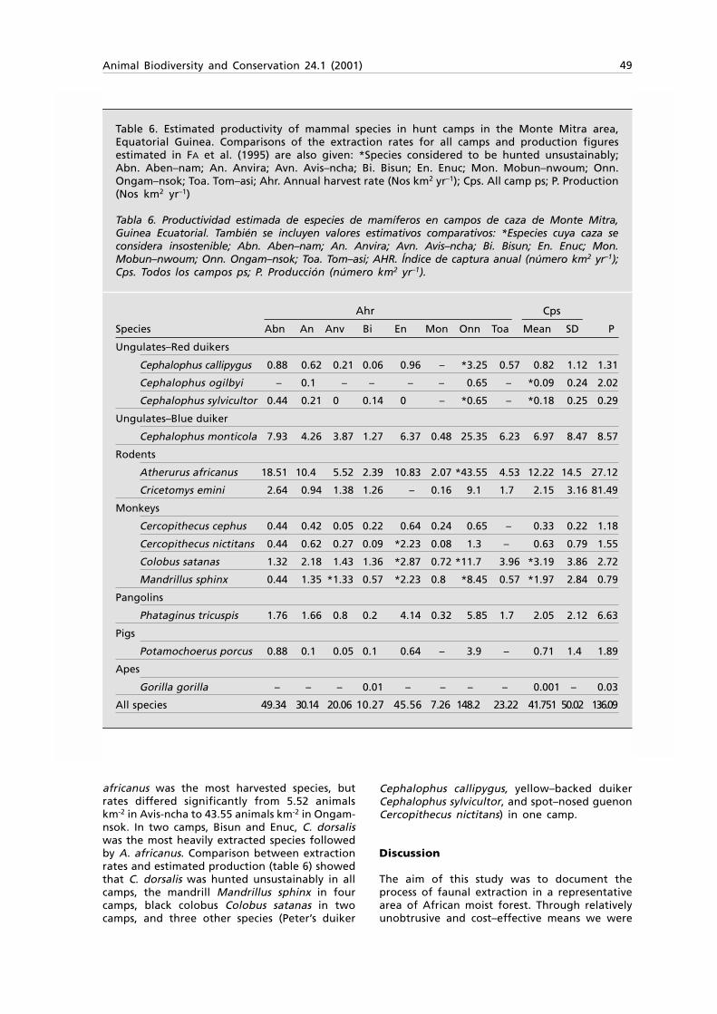
Animal Biodiversity and Conservation 24.1 (2001) 49
Table 6. Estimated productivity of mammal species in hunt camps in the Monte Mitra area,Equatorial Guinea. Comparisons of the extraction rates for all camps and production figuresestimated in FA et al. (1995) are also given: *Species considered to be hunted unsustainably;Abn. Aben–nam; An. Anvira; Avn. Avis–ncha; Bi. Bisun; En. Enuc; Mon. Mobun–nwoum; Onn.Ongam–nsok; Toa. Tom–asi; Ahr. Annual harvest rate (Nos km2 yr–1); Cps. All camp ps; P. Production(Nos km2 yr–1)
Tabla 6. Productividad estimada de especies de mamíferos en campos de caza de Monte Mitra,Guinea Ecuatorial. También se incluyen valores estimativos comparativos: *Especies cuya caza seconsidera insostenible; Abn. Aben–nam; An. Anvira; Avn. Avis–ncha; Bi. Bisun; En. Enuc; Mon.Mobun–nwoum; Onn. Ongam–nsok; Toa. Tom–asi; AHR. Índice de captura anual (número km2 yr–1);Cps. Todos los campos ps; P. Producción (número km2 yr–1).
Ahr Cps
Species Abn An Anv Bi En Mon Onn Toa Mean SD P
Ungulates–Red duikers
Cephalophus callipygus 0.88 0.62 0.21 0.06 0.96 – *3.25 0.57 0.82 1.12 1.31
Cephalophus ogilbyi – 0.1 – – – – 0.65 – *0.09 0.24 2.02
Cephalophus sylvicultor 0.44 0.21 0 0.14 0 – *0.65 – *0.18 0.25 0.29
Ungulates–Blue duiker
Cephalophus monticola 7.93 4.26 3.87 1.27 6.37 0.48 25.35 6.23 6.97 8.47 8.57
Rodents
Atherurus africanus 18.51 10.4 5.52 2.39 10.83 2.07 *43.55 4.53 12.22 14.5 27.12
Cricetomys emini 2.64 0.94 1.38 1.26 – 0.16 9.1 1.7 2.15 3.16 81.49
Monkeys
Cercopithecus cephus 0.44 0.42 0.05 0.22 0.64 0.24 0.65 – 0.33 0.22 1.18
Cercopithecus nictitans 0.44 0.62 0.27 0.09 *2.23 0.08 1.3 – 0.63 0.79 1.55
Colobus satanas 1.32 2.18 1.43 1.36 *2.87 0.72 *11.7 3.96 *3.19 3.86 2.72
Mandrillus sphinx 0.44 1.35 *1.33 0.57 *2.23 0.8 *8.45 0.57 *1.97 2.84 0.79
Pangolins
Phataginus tricuspis 1.76 1.66 0.8 0.2 4.14 0.32 5.85 1.7 2.05 2.12 6.63
Pigs
Potamochoerus porcus 0.88 0.1 0.05 0.1 0.64 – 3.9 – 0.71 1.4 1.89
Apes
Gorilla gorilla – – – 0.01 – – – – 0.001 – 0.03
All species 49.34 30.14 20.06 10.27 45.56 7.26 148.2 23.22 41.751 50.02 136.09
africanus was the most harvested species, butrates differed significantly from 5.52 animalskm-2 in Avis-ncha to 43.55 animals km-2 in Ongam-nsok. In two camps, Bisun and Enuc, C. dorsaliswas the most heavily extracted species followedby A. africanus. Comparison between extractionrates and estimated production (table 6) showedthat C. dorsalis was hunted unsustainably in allcamps, the mandrill Mandrillus sphinx in fourcamps, black colobus Colobus satanas in twocamps, and three other species (Peter’s duiker
Cephalophus callipygus, yellow–backed duikerCephalophus sylvicultor, and spot–nosed guenonCercopithecus nictitans) in one camp.
Discussion
The aim of this study was to document theprocess of faunal extraction in a representativearea of African moist forest. Through relativelyunobtrusive and cost–effective means we were
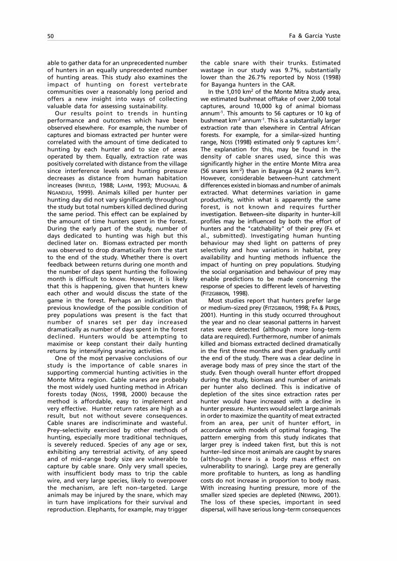
50 Fa & García Yuste
able to gather data for an unprecedented numberof hunters in an equally unprecedented numberof hunting areas. This study also examines theimpact of hunting on forest vertebratecommunities over a reasonably long period andoffers a new insight into ways of collectingvaluable data for assessing sustainability.
Our results point to trends in huntingperformance and outcomes which have beenobserved elsewhere. For example, the number ofcaptures and biomass extracted per hunter werecorrelated with the amount of time dedicated tohunting by each hunter and to size of areasoperated by them. Equally, extraction rate waspositively correlated with distance from the villagesince interference levels and hunting pressuredecreases as distance from human habitationincreases (INFIELD, 1988; LAHM, 1993; MUCHAAL &NGANDJUI, 1999). Animals killed per hunter perhunting day did not vary significantly throughoutthe study but total numbers killed declined duringthe same period. This effect can be explained bythe amount of time hunters spent in the forest.During the early part of the study, number ofdays dedicated to hunting was high but thisdeclined later on. Biomass extracted per monthwas observed to drop dramatically from the startto the end of the study. Whether there is overtfeedback between returns during one month andthe number of days spent hunting the followingmonth is difficult to know. However, it is likelythat this is happening, given that hunters kneweach other and would discuss the state of thegame in the forest. Perhaps an indication thatprevious knowledge of the possible condition ofprey populations was present is the fact thatnumber of snares set per day increaseddramatically as number of days spent in the forestdeclined. Hunters would be attempting tomaximise or keep constant their daily huntingreturns by intensifying snaring activities.
One of the most pervasive conclusions of ourstudy is the importance of cable snares insupporting commercial hunting activities in theMonte Mitra region. Cable snares are probablythe most widely used hunting method in Africanforests today (NOSS, 1998, 2000) because themethod is affordable, easy to implement andvery effective. Hunter return rates are high as aresult, but not without severe consequences.Cable snares are indiscriminate and wasteful.Prey–selectivity exercised by other methods ofhunting, especially more traditional techniques,is severely reduced. Species of any age or sex,exhibiting any terrestrial activity, of any speedand of mid–range body size are vulnerable tocapture by cable snare. Only very small species,with insufficient body mass to trip the cablewire, and very large species, likely to overpowerthe mechanism, are left non–targeted. Largeanimals may be injured by the snare, which mayin turn have implications for their survival andreproduction. Elephants, for example, may trigger
the cable snare with their trunks. Estimatedwastage in our study was 9.7%, substantiallylower than the 26.7% reported by NOSS (1998)for Bayanga hunters in the CAR.
In the 1,010 km2 of the Monte Mitra study area,we estimated bushmeat offtake of over 2,000 totalcaptures, around 10,000 kg of animal biomassannum-1. This amounts to 56 captures or 10 kg ofbushmeat km-2 annum-1. This is a substantially largerextraction rate than elsewhere in Central Africanforests. For example, for a similar–sized huntingrange, NOSS (1998) estimated only 9 captures km-2.The explanation for this, may be found in thedensity of cable snares used, since this wassignificantly higher in the entire Monte Mitra area(56 snares km-2) than in Bayanga (4.2 snares km-2).However, considerable between–hunt catchmentdifferences existed in biomass and number of animalsextracted. What determines variation in gameproductivity, within what is apparently the sameforest, is not known and requires furtherinvestigation. Between–site disparity in hunter–killprofiles may be influenced by both the effort ofhunters and the "catchability" of their prey (FA etal., submitted). Investigating human huntingbehaviour may shed light on patterns of preyselectivity and how variations in habitat, preyavailability and hunting methods influence theimpact of hunting on prey populations. Studyingthe social organisation and behaviour of prey mayenable predictions to be made concerning theresponse of species to different levels of harvesting(FITZGIBBON, 1998).
Most studies report that hunters prefer largeor medium–sized prey (FITZGIBBON, 1998; FA & PERES,2001). Hunting in this study occurred throughoutthe year and no clear seasonal patterns in harvestrates were detected (although more long–termdata are required). Furthermore, number of animalskilled and biomass extracted declined dramaticallyin the first three months and then gradually untilthe end of the study. There was a clear decline inaverage body mass of prey since the start of thestudy. Even though overall hunter effort droppedduring the study, biomass and number of animalsper hunter also declined. This is indicative ofdepletion of the sites since extraction rates perhunter would have increased with a decline inhunter pressure. Hunters would select large animalsin order to maximize the quantity of meat extractedfrom an area, per unit of hunter effort, inaccordance with models of optimal foraging. Thepattern emerging from this study indicates thatlarger prey is indeed taken first, but this is nothunter–led since most animals are caught by snares(although there is a body mass effect onvulnerability to snaring). Large prey are generallymore profitable to hunters, as long as handlingcosts do not increase in proportion to body mass.With increasing hunting pressure, more of thesmaller sized species are depleted (NEWING, 2001).The loss of these species, important in seeddispersal, will have serious long–term consequences

Animal Biodiversity and Conservation 24.1 (2001) 51
on the forest ecosystem (WRIGHT et al., 2000;MOORE, 2001).
Inter–hunter variation in number of animalshunted was considerable in the Monte Mitra area.Essentially, extraction of game was directlyproportional to the amount of time dedicated tohunting. All hunters in the study hunted game forprofit and were dedicated full–time to this activity.An average of around 70% of all game huntedwas sold by the hunter. Because of the detrimentaleffects of cable snares on wildlife, most CentralAfrican nations have banned this method. In thecase of Equatorial Guinea this is not the case, butif cable snares had not been used in Monte Mitraduring this study, only less than 9% of thedocumented prey would have been taken. Theimportance of snare hunting in increasingprofitability for the hunter is then clear.
Wildlife populations in Monte Mitra declinedunder the heavy hunting pressure during thestudy period. If they stabilised at new and lowerlevels, then current hunting may be sustainable,although this is unlikely given the emphasis onselling the meat to the Bata market. Alternatively,if hunting pressure of a site is not too intense,adjacent large tracts of undisturbed forest canbuffer and replenish hunted areas, restockinggame populations and therefore contributing tothe sustainability of hunting in an area (FA &PERES, 2001). However, heavy hunting pressure,deforestation and habitat fragmentation of manyareas disrupt the source-sink dynamics (NOVARO etal., 2000), leading to potential over–exploitationof populations. Our estimates of sustainability ofa number of game species indicate that currentlymost species are overharvested.
Conservation of the Monte Mitra region isimpossible unless the hunting for profit issue inSendje and adjoining villages is resolved.Conservationists will need to work with localresidents, who have few alternative methods forfinding food and earning an income, to find asolution to game exploitation. Bans on cablesnares may be totally unenforceable by thereduced number of park guards operating in theMonte Alén national park, and equally suchmeasures will generate considerable antagonism.Firearms may be permissible but are not a goodalternative because of the costs involved andbecause of the much lower returns. The challengeis to reduce current levels of hunting andintegrate human needs and expectations withinconservation objectives for the region (NOSS, 1997;EVES & RUGGIERO, 2001).
Acknowledgements
The fieldwork reported in this study wasundertaken as part of the Proyecto CUREF in RioMuni. We are most grateful to staff at the MonteAlén National Park, especially wardens JoséNdong and Julián Nsihi, for field assistance. We
would also like to acknowledge the help andsupport of Adolfo Ncogo in mapping huntcatchments, and in providing us with invaluablelogistic support during our visits. Manuelcollected offtake data during the entire studyperiod. We would also like to thank the hunterswho contributed information to the study. Wethank Guy Cowlishaw, John Oates and HelenNewing for comments on the manuscript.
References
ALVARD, M. S., 1994. Conservation by nativepeoples: prey choice in a depleted habitat.Human Nature, 55555: 127–154.
APE ALLIANCE, 1998. Bushmeat: A recipe forextinction. Fauna and Flora International,Cambridge.
BENNETT, E. L. & ROBINSON, J. G., 2000. Hunting forsustainability: The start of a synthesis. In:Hunting for sustainability in tropical forests:499–519 (J. G. Robinson & E. L. Bennett, Eds.).Columbia University Press, New York.
BEUDELS, R., 1998. Appui au développement d’unetypologie de habitats et pour le rassemblementdes donées faunistiques. Rapport de Synthèse,Informe Técnico CUREF–SUC.26, Bata, EquatorialGuinea.
EVES, H. E. & RUGGIERO, R. G., 2000. Socioeconomicsand the sustainability of hunting in the forestsof northern Congo (Brazzaville). In: Huntingfor sustainability in tropical forests: 427–454.(J. G. Robinson & E. L. Bennett, Eds.) ColumbiaUniversity Press, Columbia.
FA, J. E., 1991. Conservación de los ecosistemasforestales de Guinea Ecuatorial. IUCN,Cambridge and Gland.
– 2000. Hunted animals in Bioko Island, WestAfrica: sustainability and future. In: Huntingfor sustainability in tropical forests: 165–195.(J. G. Robinson & E. L. Bennett, Eds.) ColumbiaUniversity Press, Columbia.
FA, J. E., GARCÍA YUSTE, J. E. & CASTELO, R., 2000.Bushmeat markets in Bioko Island as a measure ofhunting pressure. Conserv. Biol., 14: 1,602–1,613.
FA, J. E., JUSTE, J., PEREZ DEL VAL, J. & CASTROVIEJO,J., 1995. Impact of market hunting on mammalspecies in Equatorial Guinea. Conserv. Biol., 9:1,107–1,115.
FA, J. E. & PERES, C. A., 2001. Game vertebrateextraction in African and Neotropical forests: anintercontinental comparison. In: Conservationof exploited species: 203–241 (J. D. Reynolds, G.M. Mace, J. G. Robinson, & K. H. Redford, Eds.).Cambridge University Press, Cambridge.
FA, J. E. & PURVIS, A., 1997. Body size, diet andpopulation density in Afrotropical forestmammals: a comparison with Neotropicalspecies. J. Anim. Ecol., 66: 98–112.
FA, J. E., RYAN, S. & BELL, D. J. (submitted). Generalpatterns and inter–sote variation in bushmeathunting in Afrotropical Forests. Conserv. Biol.
52 Fa & García Yuste
FITZGIBBON, C., 1998. The management of subsistenceharvesting: behavioural ecology of hunters andtheir mammalian prey. In: Behavioral ecologyand conservation biology: 449–473 (T. Caro, Ed.).Oxford University Press, Oxford.
GARCIA YUSTE, J. E. & ENEME, F., 1997. Diagnósticode las áreas críticas para la conservación.CUREF–SUC.2, Bata: Equatorial Guinea.
HART, J., 2000. Impact of sustainability ofindigenous hunting in the Ituri forest, Congo-Zaire: A comparison of unhunted and huntedduiker populations In: Hunting for sustainabilityin tropical forests: 106–153 (J. G. Robinson & E.L. Bennett, Eds.). Columbia University Press,Columbia.
INFIELD, M., 1988. Hunting, trapping and fishingin villages within and on the periphery of theKorup National Park. WWF Publication 3206/A9.6, Goldaming, UK.
JUSTE, J., FA, J. E., PEREZ DEL VAL, J., & CASTROVIEJO, J.,1995. Market dynamics of bushmeat species inEquatorial Guinea. J. Appl. Ecol., 32: 454–467.
KINGDON, J., 1997. The Kingdon field guide ofAfrican mammals. Academic Press, London.
LAHM, S. A., 1993. Ecology and economics ofhuman/wildlife interaction in northeasternGabon. Ph. D. Thesis, Univ. of New York.
MOORE, P. D., 2001. The rising cost of bushmeat.Nature, 409: 775–777.
MUCHAAL, P. K. & NGANDJUI, G., 1999. Impact ofvillage hunting on wildlife populations in thewestern Dja Reserve, Cameroon. Conserv. Biol.,13: 385–396.
NEWING, H., 2001. Bushmeat hunting andmanagement: implications of duiker ecologyand interspecific competition. Biodivers. andConserv., 10: 99–118.
NOSS, A. J., 1997. Challenges to nature conservationwith community development in central Africanforests. Oryx, 31: 180–188.
– 1998. The impacts of cable snare hunting onwildlife populations in the forests of theCentral African Republic. Conserv. Biol., 12:390–398.
– 2000. Cable snares and nets in the CentralAfrican Republic. In: Hunting for sustainabilityin tropical forests: 106–153 (J. G. Robinson &E. L. Bennett, Eds.). Columbia University Press,Columbia.
NOVARO, A. J., REDFORD, K. H. & BODMER, R. E.,2000. Effect of hunting in source–sink systemsin the Neotropics. Conserv. Biol., 14: 713–721.
ROBINSON, J. G. & REDFORD, K. H., 1991. Sustainableharvest of Neotropical forest animals. In:Neotropical wildlife use and conservation:415–429 (J. G. Robinson & K. H. Redford,Eds.). Chicago University Press, Chicago.
ROBINSON, J. G., REDFORD, K. H. & BENNETT, E. L.,1999. Wildlife harvest in logged tropicalforests. Science, 284: 595–596.
SAYER, J. A., HARCOURT, C. S. & COLINS, N. M., 1992.The conservation atlas of tropical forests:Africa. Macmillan Publishers, Basingstoke.
VENABLES, W. N. & RIPLEY, B. D., 1999. Modern appliedstatistics with S–Plus. Springer–Verlag, Berlin.
WILKIE, D. S. & CARPENTER, J. F., 1999. Bushmeathunting in the Congo Basin: an assessment ofimpacts and options for mitigation. Biodiv.and Conserv., 8: 927–955.
WRIGHT, S. J., ZEBALLOS, H., DOMÍNGUEZ, I., GALLARDO,M. M., MORENO, M. C. & IBAÑEZ, R., 2000.Poachers alter mammal abundance, seeddispersal, and seed predation in a Neotropicalforest. Conserv. Biol., 14: 227–239.

53Animal Biodiversity and Conservation 24.1 (2001)
© 2001 Museu de ZoologiaISSN: 1578–665X
Composición y calidad de la dietadel ciervo (Cervus elaphus L.)en el norte de la península ibérica
I. Garin, A. Aldezabal, R. García–González &J. R. Aihartza
Garin, I, Aldezabal, A., García–González, R. & Aihartza, J. R., 2001. Composición y calidad de la dieta del ciervo(Cervus elaphus L.) en el norte de la península ibérica. Animal Biodiversity and Conservation, 24.1: 53–63.
AbstractAbstractAbstractAbstractAbstractPlant composition and quality of the red deer (Cervus elaphus L.) diet in the northern Iberian peninsula.—Thefeeding pattern of red deer varies greatly among the different European populations. The aim of our study wasto elucidate the plant composition and the quality of the red deer diet in the Pyrenees (Northern Iberianpeninsula). Over a one–year period, the red deer fed mainly on browse, pines being the main food. However,unlike other populations on the Iberian peninsula, consumption of herbaceous plants was higher than browsein the spring–summer period. Nevertheless, the diet of Pyrenean red deer shared some features with theMediterranean populations such as browsing on woody legumes. Fecal nitrogen content, as an index of dietquality, showed low annual values with a marked decrease in winter. The overall feeding pattern was similar tothat of other Central European populations. The large size of the surveyed population probably affected its highlevel of browse consumption and poor quality diet.
Key words: Diet, Red deer, Plant composition, Quality.
ResumenResumenResumenResumenResumenComposición vegetal y calidad de la dieta del ciervo (Cervus elaphus L.) en el norte de la península Ibérica.—El patrón de alimentación del ciervo es muy variable entre las diferentes poblaciones europeas. El objetivo denuestro estudio fue determinar la composición vegetal y la calidad de la dieta del ciervo en los Pirineos (nortede la península Ibérica). Durante un periodo de un año, el ciervo se alimentó principalmente de plantas leñosas,siendo los pinos su principal alimento. Sin embargo a diferencia de otras poblaciones de la península Ibérica, elconsumo de plantas herbáceas fue superior al de leñosas en primavera y verano. No obstante, la dieta del ciervodel Pirineo comparte algunas características con la de las poblaciones mediterráneas, como el consumo deplantas leguminosas leñosas. El contenido en nitrógeno fecal, como índice de calidad de la dieta, presentavalores anuales bajos con una marcada disminución en invierno. El patrón de alimentación global fue similar alde otras poblaciones centroeuropeas. El gran tamaño de la población estudiada influye probablemente en elalto nivel de consumo de leñosas y la baja calidad de su dieta.
Palabras clave: Dieta, Ciervo, Composición vegetal, Calidad.
(Received: 31 I 01; Conditional acceptance: 13 VI 01; Final acceptance: 3 VII 01)
I. Garin & J. R. Aihartza, Zoologia eta Animali Zelulen Dinamika Saila, UPV/EHU, 644 PK, 48080 Bilbo, BasqueCountry, España (Spain).– A. Aldezabal, Landare–Biologia eta Ekologia Saila, UPV/EHU, 644 PK, 48080 Bilbo,Basque Country, España (Spain).– R. García–González, Instituto Pirenaico de Ecología (CSIC), Apdo. 64, 22700Jaca, España (Spain).
54 Garin et al.
Introducción
La valoración del impacto del ciervo (Cervuselaphus) sobre los ecosistemas ha dado lugar anumerosos trabajos sobre sus hábitos alimen-tarios. Las primeras revisiones constataron laenorme variabilidad en la preferencia por lasdistintas especies vegetales, a partir de las cua-les se intentó generalizar una clasificación deespecies preferidas por el ciervo (KAY & STAINES,1981). Así, algunos autores han constatado queel alimento más importante en la dieta delciervo a lo largo del año son las especies leño-sas de hoja caduca (DZIECIOLOWSKI, 1969); porotra parte, otros autores han enumerado unaserie de especies clave para la dieta del ciervo(GOFFIN & DE CROMBRUGGHE, 1976). Probablemen-te, la plasticidad en el comportamientoalimentario del ciervo, definido como pastador–ramoneador (HOFMANN, 1989), le permita ade-cuar fácilmente el consumo de las diferentescategorías vegetales a los cambios tanto tem-porales como espaciales o geográficos de ladisponibilidad de los recursos alimentarios.
Las herbáceas son generalmente más abun-dantes en la dieta primaveral, mientras que laimportancia de las leñosas aumenta a medidaque nos adentramos en el otoño y el invierno(MITCHELL et al., 1977). Los diferentes regíme-nes de precipitación y temperatura en Europadan lugar a variados patrones fenológicos delos grupos de plantas consumidas: por ejem-plo, el comienzo tardío del periodo vegetativode las latitudes más septentrionales condicionaque las herbáceas alcancen su máximo en lacomposición de la dieta durante el verano(MITCHELL et al., 1977); mientras que en regionesmediterráneas el máximo puede ser a finales deinvierno o comienzos de primavera (RODRÍGUEZ–BERROCAL, 1978). La nieve llega a hacer anecdóticala presencia de herbáceas en la dieta invernal(DZIECIOLOWSKI, 1969), mientras que en zonas deinfluencia oceánica o mediterránea, de inviernosmás templados, la proporción de herbáceas du-rante la época llamada desfavorable supera el20% y puede alcanzar el 50% de la dieta (JENSEN,1968; RODRÍGUEZ–BERROCAL, 1978; VENERO, 1984;GROOT–BRUINDERINK & HAZEBROEK, 1995). En laszonas deforestadas de Escocia su dieta esmayoritariamente herbácea (MITCHELL et al., 1977)y en las poblaciones polacas más forestales, lahierba es cuantitativamente poco importante enla dieta media anual (DZIECIOLOWSKI, 1969).
La mencionada plasticidad permite a la especiemantenerse en un mismo lugar a pesar de que ladisponibilidad de alimento varíe notablementede una época a otra del año y habitar ambientesvegetales radicalmente opuestos. La variaciónestacional en la alimentación está acompañadaademás de cambios en la función ruminal, queayudan a reducir el impacto de la variación de lacalidad de la dieta en la efectividad de la diges-tión (JIANG & HUDSON, 1996; LENTLE et al., 1996).
En los ungulados domésticos el descenso de lacalidad de la ingesta coincide con la reducción delas ganancias corporales de los individuos (LENG,1990; VOGEL et al., 1993). Si la calidad de la dietadel ciervo desciende por debajo de un umbral, elindividuo no satisface sus requerimientos, comen-zando a movilizar sus reservas y a perder peso(GATES & HUDSON, 1981). Por ello, la monitorizaciónde la calidad de la dieta puede ofrecer un diag-nóstico poblacional. En condiciones naturales ycon animales salvajes, los índices de calidadnutricional utilizados de forma habitual se esti-man a partir de las características químicas de lasheces (PUTMAN, 1984). Los altos requerimientos deproteína (Nx6,25) en los animales en relación a sudisponibilidad en las plantas, convierte al nitró-geno ingerido en un indicador importante de lacalidad de la dieta de los herbívoros (MATTSON,1980). La posibilidad de que el contenido denitrógeno en las heces pueda estar a su vezrelacionado con el contenido en nitrógeno de ladieta y la facilidad en la obtención de muestrasfecales, han convertido el nitrógeno fecal en uníndice muy utilizado (GOGAN & BARRET, 1994; MASSEI
et al., 1994; MERRILL et al., 1995).El patrón de variación temporal del nitrógeno
fecal está determinado principalmente por eldesarrollo fenológico de las plantas consumidas,ya que el contenido de nitrógeno en las plantasdepende de dicho factor. Así, cuando el materialvegetal se encuentra en las primeras etapas deldesarrollo, contiene el pico máximo de nitróge-no, y decae a medida que nos acercamos alinvierno (MATTSON, 1980). La misma tendenciatemporal ha sido observada en el nitrógeno fe-cal (VAN SOEST, 1994).
Al igual que otras muchas especies de cérvidos,el ciervo ha sido objeto durante los últimossiglos de numerosas reintroducciones y trasladosa lo largo del mundo, y hoy en día podemosencontrarlo fuera de su área natural de distribu-ción, como por ejemplo en Argentina, NuevaZelanda o Australia (WHITEHEAD, 1972; PUTMAN,1988). Como en otros macizos montañosos deEuropa, el ciervo también ha sido reintroducidoen ambas vertientes de los Pirineos (TEILLAUD etal., 1991). Las poblaciones de Euskal Herria,Aragón y Cataluña proceden de animales prove-nientes del sur de España y reintroducidos en losaños 50 y 60.
Aunque la alimentación del ciervo en laspoblaciones de la región mediterránea ha sidoampliamente estudiada (MARTÍNEZ 1996; ÁLVAREZ
& RAMOS, 1991; SORIGUER et al., 1994; GARCÍA–GONZÁLEZ & CUARTAS, 1992), la dieta en el nortede la península ibérica es prácticamentedesconocida.
El objetivo del presente estudio ha sido cubrirese vacío en el conocimiento del ciervo, investi-gando su dieta y calidad en una población pire-naica. Por otro lado, se pretende determinar elmodelo trófico (centroeuropeo o Mediterráneo)al que pertenece el ciervo en el, Pirineo dado
Animal Biodiversity and Conservation 24.1 (2001) 55
que las características geográficas de ambas re-giones confluyen en este área. Asímismo, se havalorado y discutido sus hábitos alimentariosestacionales en relación a las características nu-tritivas de la vegetación.
Área de estudio
El presente trabajo se ha realizado en los vallesde La Garcipollera y Cenarbe (norte de Huesca),que conforman la Reserva de Caza de LaGarcipollera de 55,8 km2 de extensión. La preci-pitación anual es 1.051 mm y la temperaturamedia anual 9,7°C. Los meses de verano son losmás secos y las temperaturas medias de los me-ses invernales superiores a los 0°C. La zona seencuentra entre los 850 m y los 2.200 m dealtitud y está prácticamente deshabitada en laactualidad. La vegetación está constituida princi-palmente por repoblaciones de negral de Austria(Pinus nigra subsp. nigra) y de pino albar (P.sylvestris), abetares (Abies alba) de reducida exten-sión, quejigares (Quercus humilis), algunos pradosy los pastos supraforestales. La población de cier-vos procede de reintroducciones realizadas en losaños 60 con 37 individuos procedentes de losMontes de Toledo. A mediados de los años 90 seestimó que la densidad era de 35 ind./km2, la sex–ratio de tres hembras por macho y la fertilidaddel 51% (MARCO et al., 1996; GARIN, 1997). No sehan observado corzos (Capreolus capreolus) enla reserva y los jabalíes (Sus scrofa) son probable-mente abundantes debido a la ausencia de caza(GARIN, 1997).
Material y métodos
Dieta
La composición de la dieta del ciervo se determi-nó mediante el análisis microhistológico de lasheces (SPARKS & MALECHEK, 1968; HOLECHEK et al.,1982; CUARTAS & GARCÍA–GONZÁLEZ, 1996). Estemétodo permite estudiar la dieta de una especieanimal sin causar ninguna molestia a los indivi-duos y es apto para medios con escasa visibili-dad, donde existen dificultades para observardirectamente los hábitos alimentarios de la es-pecie. La aparición de fragmentos vegetales enlas heces depende de su resistencia a ladegradabilidad durante los procesos digestivosdel herbívoro. Por ello, las epidermis de las espe-cies menos resistentes se ven subestimadas res-pecto a otras con mayor grado de resistencia.Aquellas partes de la planta que por carecer decaracterísticas específicas son difícilmenteidentificables en las heces (p.e. las partes leño-sas), se subestiman igualmente (HOLECHEK &VALDEZ, 1985). En consecuencia, este método norefleja de forma precisa la cantidad relativa decada especie o grupo de especies consumida porel animal (PUTMAN, 1984). La técnica micro-
histológica permite, sin embargo, clasificar lasplantas consumidas por el herbívoro según suorden de importancia en la dieta y seguir suvariación temporal y su diversidad (CUARTAS &GARCÍA–GONZÁLEZ, 1996).
Desde mayo de 1993 hasta abril de 1994 serecogieron mensualmente en 4 estaciones demuestreo un mínimo de 9 deposiciones fecalesfrescas por estación, correspondiente a indivi-duos adultos (según ÁLVAREZ, 1994). En una delas estaciones no pudieron recogerse excremen-tos en mayo y tampoco pudieron recolectarse enninguna de ellas durante junio. La localizaciónde las estaciones de recogida reflejó la diversi-dad de ambientes altitudinales y vegetales delárea de estudio.
Los excrementos se guardaron en bolsas deplástico, que se congelaron a –20°C hasta suprocesamiento. Tras la homogeneización de lasdeposiciones, se separaron 5cc de cada deposi-ción que se mezclaron de acuerdo a su estacióny mes de muestreo. La contribución de materialfecal de cada deposición a la mezcla fue similar.Las mezclas se prepararon siguiendo el protoco-lo de CUARTAS (1992) y se guardaron enacetoformol antes de la identificación de lasepidermis vegetales. Para el conteo de cutículasse prepararon cinco portaobjetos por mezcla ymes, y en la medida que fue posible, se identi-ficaron hasta el nivel de especie todas las epi-dermis interceptadas a lo largo de tres transectosdispuestos regularmente en el porta (SEBER &PEMBERTON, 1979).
Las epidermis se clasificaron en tres grupos:1. Graminoides, en las que se incluyen lasgramíneas, las ciperáceas y las juncáceas; 2. Dico-tiledóneas, en las que se incluyen todas las plan-tas herbáceas correspondientes a este grupo máslas monocotiledóneas no gramínoides (es decir,liliaceas, iridáceas, orquídeas,…); 3. Leñosas, tan-to de porte arbustivo como arbóreo.
Debido a que la determinación de forma unifi-cada de la disponibilidad del estrato herbáceo ydel estrato leñoso no estuvo al alcance del equipode trabajo, no se ha podido realizar un análisiscuantitativo de la selección de la dieta.
Nitrógeno fecal
Hemos valorado la calidad de la dieta del ciervoa través del nitrógeno de las heces asumiendoque el nitrógeno fecal y el nitrógeno de la dietaestán relacionados (LESLIE & STARKEY, 1985;PUTMAN & HEMMINGS, 1986; IRWIN et al., 1993). Elnitrógeno fecal tendría una respuesta sigmoidala las variaciones del nitrógeno de la dieta:cuando el contenido del nitrógeno de la dietaes alto el nitrógeno puede ser tóxico y por ellose excretaría relativamente más; por el contra-rio, cuando el nitrógeno de la dieta es muy bajose incrementa la capacidad de retención. Entramos cortos de variación del nitrógeno en ladieta la relación entre el nitrógeno de la dieta

56 Garin et al.
y nitrógeno fecal sería lineal (PUTMAN, 1984).Esta relación lineal depende, sin embargo, devarios factores, como el contenido en taninos,la digestibilidad del alimento o el estado fisio-lógico del animal (HOBBS, 1987; ROBBINS et al.,1987; HOWERY & PFISTER, 1990). Sin embargo, suefecto sobre la relación entre el nitrógenofecal y el nitrógeno de la dieta en ambientenatural puede no ser tan importante (MOULD &ROBBINS, 1981; HANLEY et al., 1992; CAUGHLEY &SINCLAIR, 1994) lo que permite el uso del nitró-geno fecal como valor indicativo de la calidadde la dieta.
Debido a que las inclemencias meteorológi-cas y el lavado del nitrógeno de la muestrafecal previo a su recolección afecta el valor delnitrógeno fecal, la recolección de heces deberealizarse antes de 24 días a partir de su depo-sición (JENKS et al., 1990). En nuestro caso, laapariencia de las muestras (color, brillo y muco-sidad) aseguró su recolección en menos de unasemana desde su deposición.
Parte de las deposiciones se secaron en estu-fa a 90°C, se molieron hasta obtener partículasmenores a 1 mm, y se guardaron en bolsa deplástico previo a su análisis, según el procedi-miento de Kjeldahl.
ResultadosResultadosResultadosResultadosResultados
Composición florística de la dieta
En total se recogieron 791 deposiciones y seidentificaron 18.093 fragmentos vegetales, esdecir, una media de 421 por mes y estación demuestreo.
En el total anual, el 51% de los fragmen-tos vegetales corresponde a la fracción leño-sa (Intérvalo de Confianza, IC = 57%÷45%),siendo el grupo de plantas más consumido,seguido de las graminoides (x = 36%,IC = 40%÷32%) y por último las dicotiledóneasfueron las menos representadas en la dieta(x = 10%, IC = 13%÷7%)
La variación mensual de los tres tipos deplantas consumidos se ha representado en lafigura 1. El alimento leñoso tiene un pesoimportante a lo largo de todo el año, conmáximo invernal —durante enero y febrero lasplantas de origen leñoso sobrepasaron las trescuartas partes de las epidermis determinada—y mínimo entre abril y septiembre —únicamen-te una cuarta parte en julio— que correspondea la época en la que las herbáceas cobranmayor importancia en la dieta del ciervo de La
Graminoides Dicotiledóneas Leñosas Graminoides Dicotiledóneas Leñosas Graminoides Dicotiledóneas Leñosas Graminoides Dicotiledóneas Leñosas Graminoides Dicotiledóneas Leñosas
100100100100100
8080808080
6060606060
4040404040
2020202020
00000 5 7 8 9 10 11 12 1 2 3 4
Mes Mes Mes Mes Mes
% % % % %
Fig. 1. Variación mensual del porcentaje de los grupos de plantas en los excrementos de ciervode La Garcipollera.
Fig. 1. Monthly variation of the percentage of plant groups in the fecal pellets of red deer fromLa Garcipollera.
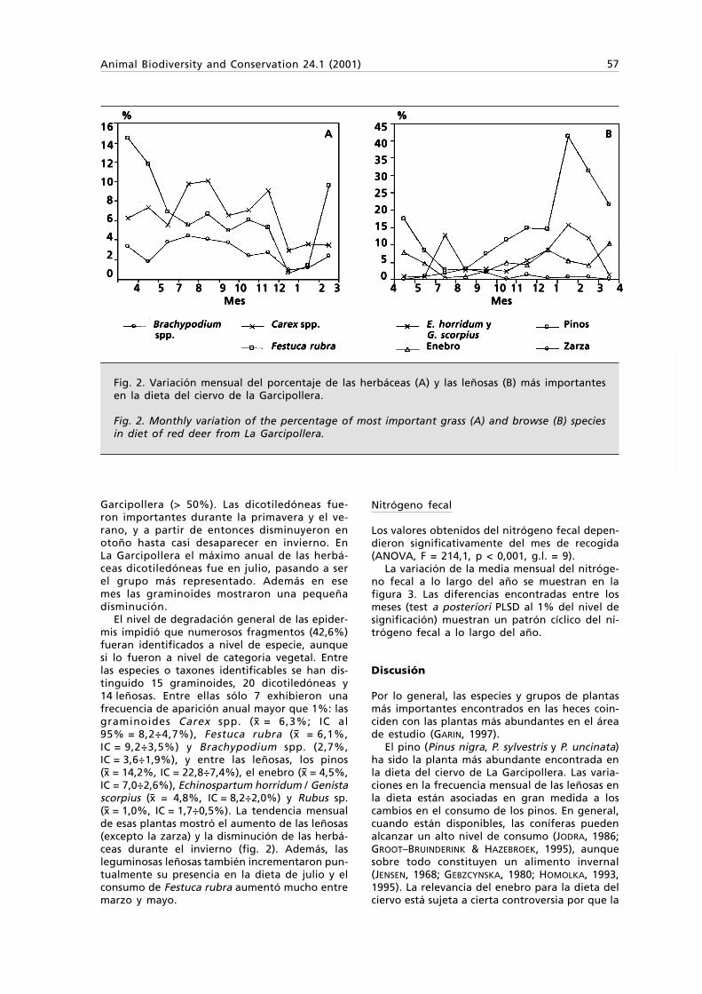
Animal Biodiversity and Conservation 24.1 (2001) 57
Garcipollera (> 50%). Las dicotiledóneas fue-ron importantes durante la primavera y el ve-rano, y a partir de entonces disminuyeron enotoño hasta casi desaparecer en invierno. EnLa Garcipollera el máximo anual de las herbá-ceas dicotiledóneas fue en julio, pasando a serel grupo más representado. Además en esemes las graminoides mostraron una pequeñadisminución.
El nivel de degradación general de las epider-mis impidió que numerosos fragmentos (42,6%)fueran identificados a nivel de especie, aunquesi lo fueron a nivel de categoria vegetal. Entrelas especies o taxones identificables se han dis-tinguido 15 graminoides, 20 dicotiledóneas y14 leñosas. Entre ellas sólo 7 exhibieron unafrecuencia de aparición anual mayor que 1%: lasgraminoides Carex spp. (x = 6,3%; IC al95% = 8,2÷4,7%), Festuca rubra (x = 6,1%,IC = 9,2÷3,5%) y Brachypodium spp. (2,7%,IC = 3,6÷1,9%), y entre las leñosas, los pinos(x = 14,2%, IC = 22,8÷7,4%), el enebro (x = 4,5%,IC = 7,0÷2,6%), Echinospartum horridum / Genistascorpius (x = 4,8%, IC = 8,2÷2,0%) y Rubus sp.(x = 1,0%, IC = 1,7÷0,5%). La tendencia mensualde esas plantas mostró el aumento de las leñosas(excepto la zarza) y la disminución de las herbá-ceas durante el invierno (fig. 2). Además, lasleguminosas leñosas también incrementaron pun-tualmente su presencia en la dieta de julio y elconsumo de Festuca rubra aumentó mucho entremarzo y mayo.
Nitrógeno fecal
Los valores obtenidos del nitrógeno fecal depen-dieron significativamente del mes de recogida(ANOVA, F = 214,1, p < 0,001, g.l. = 9).
La variación de la media mensual del nitróge-no fecal a lo largo del año se muestran en lafigura 3. Las diferencias encontradas entre losmeses (test a posteriori PLSD al 1% del nivel designificación) muestran un patrón cíclico del ni-trógeno fecal a lo largo del año.
Discusión
Por lo general, las especies y grupos de plantasmás importantes encontrados en las heces coin-ciden con las plantas más abundantes en el áreade estudio (GARIN, 1997).
El pino (Pinus nigra, P. sylvestris y P. uncinata)ha sido la planta más abundante encontrada enla dieta del ciervo de La Garcipollera. Las varia-ciones en la frecuencia mensual de las leñosas enla dieta están asociadas en gran medida a loscambios en el consumo de los pinos. En general,cuando están disponibles, las coníferas puedenalcanzar un alto nivel de consumo (JODRA, 1986;GROOT–BRUINDERINK & HAZEBROEK, 1995), aunquesobre todo constituyen un alimento invernal(JENSEN, 1968; GEBZCYNSKA, 1980; HOMOLKA, 1993,1995). La relevancia del enebro para la dieta delciervo está sujeta a cierta controversia por que la
Fig. 2. Variación mensual del porcentaje de las herbáceas (A) y las leñosas (B) más importantesen la dieta del ciervo de la Garcipollera.
Fig. 2. Monthly variation of the percentage of most important grass (A) and browse (B) speciesin diet of red deer from La Garcipollera.
AAAAA B B B B B1616161616
1414141414
1212121212
1010101010
88888
66666
44444
22222
00000
4545454545
4040404040
3535353535
3030303030
2525252525
2020202020
1515151515
1010101010
55555
000004 54 54 54 54 5 7 8 9 7 8 9 7 8 9 7 8 9 7 8 9 10 11 12 10 11 12 10 11 12 10 11 12 10 11 12 11111 2 3 2 3 2 3 2 3 2 3 4 4 4 4 4 5 5 5 5 5 7 8 9 7 8 9 7 8 9 7 8 9 7 8 9 10 11 12 10 11 12 10 11 12 10 11 12 10 11 12 1 2 3 41 2 3 41 2 3 41 2 3 41 2 3 4
Mes Mes Mes Mes Mes Mes Mes Mes Mes Mes
BrachypodiumBrachypodiumBrachypodiumBrachypodiumBrachypodium Carex Carex Carex Carex Carex spp. spp. spp. spp. spp. E. horridum E. horridum E. horridum E. horridum E. horridum yyyyy PinosPinosPinosPinosPinos spp. spp. spp. spp. spp. G. scorpiusG. scorpiusG. scorpiusG. scorpiusG. scorpius
Festuca rubraFestuca rubraFestuca rubraFestuca rubraFestuca rubra EnebroEnebroEnebroEnebroEnebro Zarza Zarza Zarza Zarza Zarza
% % % % % % % % % %
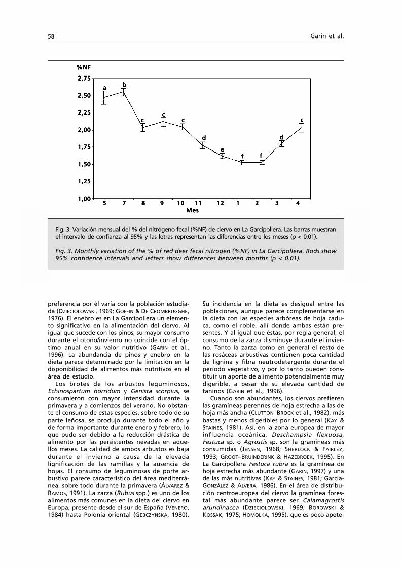
58 Garin et al.
preferencia por él varía con la población estudia-da (DZIECIOLOWSKI, 1969; GOFFIN & DE CROMBRUGGHE,1976). El enebro es en La Garcipollera un elemen-to significativo en la alimentación del ciervo. Aligual que sucede con los pinos, su mayor consumodurante el otoño/invierno no coincide con el óp-timo anual en su valor nutritivo (GARIN et al.,1996). La abundancia de pinos y enebro en ladieta parece determinado por la limitación en ladisponibilidad de alimentos más nutritivos en elárea de estudio.
Los brotes de los arbustos leguminosos,Echinospartum horridum y Genista scorpius, seconsumieron con mayor intensidad durante laprimavera y a comienzos del verano. No obstan-te el consumo de estas especies, sobre todo de suparte leñosa, se produjo durante todo el año yde forma importante durante enero y febrero, loque pudo ser debido a la reducción drástica dealimento por las persistentes nevadas en aque-llos meses. La calidad de ambos arbustos es bajadurante el invierno a causa de la elevadalignificación de las ramillas y la ausencia dehojas. El consumo de leguminosas de porte ar-bustivo parece característico del área mediterrá-nea, sobre todo durante la primavera (ÁLVAREZ &RAMOS, 1991). La zarza (Rubus spp.) es uno de losalimentos más comunes en la dieta del ciervo enEuropa, presente desde el sur de España (VENERO,1984) hasta Polonia oriental (GEBCZYNSKA, 1980).
Su incidencia en la dieta es desigual entre laspoblaciones, aunque parece complementarse enla dieta con las especies arbóreas de hoja cadu-ca, como el roble, allí donde ambas están pre-sentes. Y al igual que éstas, por regla general, elconsumo de la zarza disminuye durante el invier-no. Tanto la zarza como en general el resto delas rosáceas arbustivas contienen poca cantidadde lignina y fibra neutrodetergente durante elperiodo vegetativo, y por lo tanto pueden cons-tituir un aporte de alimento potencialmente muydigerible, a pesar de su elevada cantidad detaninos (GARIN et al., 1996).
Cuando son abundantes, los ciervos prefierenlas gramíneas perennes de hoja estrecha a las dehoja más ancha (CLUTTON–BROCK et al., 1982), másbastas y menos digeribles por lo general (KAY &STAINES, 1981). Así, en la zona europea de mayorinfluencia oceánica, Deschampsia flexuosa,Festuca sp. o Agrostis sp. son la gramíneas másconsumidas (JENSEN, 1968; SHERLOCK & FAIRLEY,1993; GROOT–BRUINDERINK & HAZEBROEK, 1995). EnLa Garcipollera Festuca rubra es la gramínea dehoja estrecha más abundante (GARIN, 1997) y unade las más nutritivas (KAY & STAINES, 1981; García-GONZÁLEZ & ALVERA, 1986). En el área de distribu-ción centroeuropea del ciervo la gramínea fores-tal más abundante parece ser Calamagrostisarundinacea (DZIECIOLOWSKI, 1969; BOROWSKI &KOSSAK, 1975; HOMOLKA, 1995), que es poco apete-
Fig. 3. Variación mensual del % del nitrógeno fecal (%NF) de ciervo en La Garcipollera. Las barras muestranel intervalo de confianza al 95% y las letras representan las diferencias entre los meses (p < 0,01).
Fig. 3. Monthly variation of the % of red deer fecal nitrogen (%NF) in La Garcipollera. Rods show95% confidence intervals and letters show differences between months (p < 0.01).
55555 77777 88888 99999 1010101010 1111111111 1212121212 11111 22222 33333 44444MesMesMesMesMes
2,752,752,752,752,75
2,502,502,502,502,50
2,252,252,252,252,25
2,002,002,002,002,00
1,751,751,751,751,75
1,501,501,501,501,50
1,251,251,251,251,25
1,001,001,001,001,00
%NF%NF%NF%NF%NF
aaaaa bbbbb
cccccccccc
ccccc
ddddd
eeeeefffff fffff
ddddd
ccccc
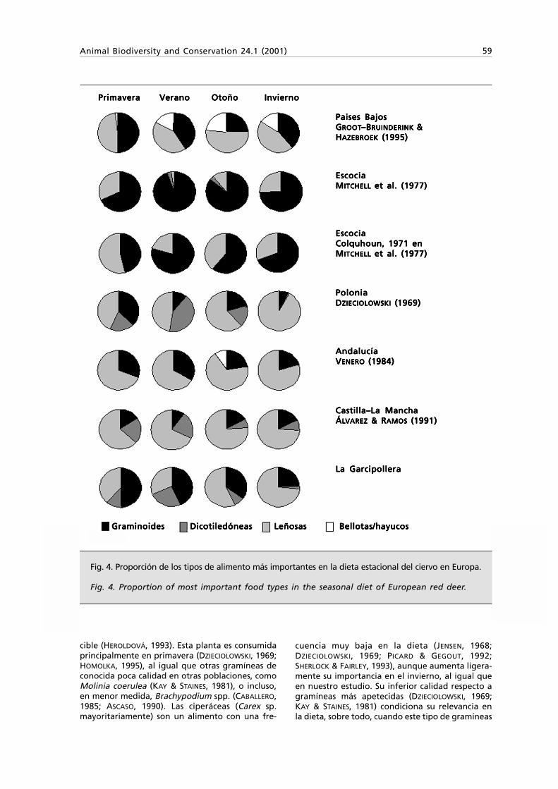
Animal Biodiversity and Conservation 24.1 (2001) 59
Fig. 4. Proporción de los tipos de alimento más importantes en la dieta estacional del ciervo en Europa.
Fig. 4. Proportion of most important food types in the seasonal diet of European red deer.
Graminoides Dicotiledóneas Leñosas Bellotas/hayucosGraminoides Dicotiledóneas Leñosas Bellotas/hayucosGraminoides Dicotiledóneas Leñosas Bellotas/hayucosGraminoides Dicotiledóneas Leñosas Bellotas/hayucosGraminoides Dicotiledóneas Leñosas Bellotas/hayucos
Primavera Primavera Primavera Primavera Primavera VVVVVerano Otoñoerano Otoñoerano Otoñoerano Otoñoerano Otoño Invierno Invierno Invierno Invierno Invierno
Paises BajosPaises BajosPaises BajosPaises BajosPaises BajosGGGGGROOTROOTROOTROOTROOT–B–B–B–B–BRUINDERINKRUINDERINKRUINDERINKRUINDERINKRUINDERINK & & & & &HHHHHAZEBROEKAZEBROEKAZEBROEKAZEBROEKAZEBROEK ( ( ( ( (1995)1995)1995)1995)1995)
EscociaEscociaEscociaEscociaEscociaMMMMMITCHELLITCHELLITCHELLITCHELLITCHELL et al. (1977) et al. (1977) et al. (1977) et al. (1977) et al. (1977)
EscociaEscociaEscociaEscociaEscociaColquhoun, 1971 enColquhoun, 1971 enColquhoun, 1971 enColquhoun, 1971 enColquhoun, 1971 enMMMMMITCHELLITCHELLITCHELLITCHELLITCHELL et al. (1977) et al. (1977) et al. (1977) et al. (1977) et al. (1977)
PoloniaPoloniaPoloniaPoloniaPoloniaDDDDDZIECIOLOWSKIZIECIOLOWSKIZIECIOLOWSKIZIECIOLOWSKIZIECIOLOWSKI ( ( ( ( (1969)1969)1969)1969)1969)
AAAAAndalucíandalucíandalucíandalucíandalucíaVVVVVENEROENEROENEROENEROENERO (1 (1 (1 (1 (1984)984)984)984)984)
Castilla–La ManchaCastilla–La ManchaCastilla–La ManchaCastilla–La ManchaCastilla–La ManchaÁÁÁÁÁLLLLLVVVVVAREZAREZAREZAREZAREZ & R & R & R & R & RAMOSAMOSAMOSAMOSAMOS ( ( ( ( (1991)1991)1991)1991)1991)
La GarcipolleraLa GarcipolleraLa GarcipolleraLa GarcipolleraLa Garcipollera
cible (HEROLDOVÁ, 1993). Esta planta es consumidaprincipalmente en primavera (DZIECIOLOWSKI, 1969;HOMOLKA, 1995), al igual que otras gramíneas deconocida poca calidad en otras poblaciones, comoMolinia coerulea (KAY & STAINES, 1981), o incluso,en menor medida, Brachypodium spp. (CABALLERO,1985; ASCASO, 1990). Las ciperáceas (Carex sp.mayoritariamente) son un alimento con una fre-
cuencia muy baja en la dieta (JENSEN, 1968;DZIECIOLOWSKI, 1969; PICARD & GEGOUT, 1992;SHERLOCK & FAIRLEY, 1993), aunque aumenta ligera-mente su importancia en el invierno, al igual queen nuestro estudio. Su inferior calidad respecto agramíneas más apetecidas (DZIECIOLOWSKI, 1969;KAY & STAINES, 1981) condiciona su relevancia enla dieta, sobre todo, cuando este tipo de gramíneas

60 Garin et al.
abundan (p. e. D. flexuosa o F. rubra). La persis-tencia vegetativa de los cárices durante el invier-no favorece probablemente su consumo, sobretodo cuando otras graminoides están secas. Porotro lado, la aparición de la nieve en LaGarcipollera a finales de diciembre de 1993 y supersistencia durante los meses de enero y febrerode 1994 estuvo ligado a un descenso brusco en lafrecuencia de los alimentos herbáceos. En laszonas más continentales, cuando la nieve cuaja ycubre el suelo las especies herbáceas disminuyenen la dieta (DZIECIOLOWSKI, 1969; JODRA, 1986; PICARD
& GEGOUT, 1992).La aparición de las quercíneas en las heces ha
sido reducida. A pesar de que la extensión de losbosques formados por el quejigo no es pequeña(399 Ha), el ramoneo en los años previos a esteestudio puede ser la causa de su baja disponibi-lidad actual, tal y como se ha sugerido para lasespecies arbóreas más preferidas en otras pobla-ciones de ciervos (DZIECIOLOWSKI, 1969; SORIGUER
et al., 1994). En la región mediterránea, cuandolos ciervos habitan bosques naturales maduros,el alimento leñoso más consumido proviene delas quercíneas (ÁLVAREZ & RAMOS, 1991; CUARTAS,1992; MARTÍNEZ, 1996). En la Europa continentaltambién el roble pedunculado (Quercus robur)es consumido todo el año cuando está presente(BOBEK et al., 1972), incluso durante el invierno(GEBCZYNSKA, 1980; MÁTRAI & KABAI, 1989; PICARD
& GEGOUT, 1992).Además de los tipos de alimento utilizados en
este estudio, algunas poblaciones aprovechantambién los frutos (de fagáceas) sobre todo enotoño e invierno (VENERO, 1984; PALACIOS et al.,1989; PICARD & GEGOUT, 1992; GROOT–BRUINDERINK
& HAZEBROEK, 1995). La diferencias en la disponi-bilidad de ese alimento pueden explicar la des-igual incidencia de la montanera en la dieta delciervo en Europa (fig. 4), aunque la coexistenciadel ciervo con alguna(s) de las muchas especiesque también utilizan los frutos forestales puedeser en parte responsable de esas diferencias. Laausencia de bellotas en la dieta del ciervo en LaGarcipollera puede deberse a que su producciónfalló en el otoño de 1993 (obs. pers.). Aunque,por otro lado, hay que considerar que la técnicade determinación microhistológica de la dietapuede no detectar los frutos de las fagáceas(ÁLVAREZ & RAMOS, 1991). El consumo otoñal delos frutos de quercíneas, que es un alimento dealta digestibilidad y contenido energético(ROBBINS, 1993; FOCARDI et al., 1995), puede ayu-dar a mejorar la condición corporal de los indivi-duos al comienzo del invierno (JACKSON, 1974). Esmás que probable que la población de LaGarcipollera recurra a las bellotas como alimen-to otoñal en los años de buena fructificación.
El valor anual del nitrógeno fecal observadoen La Garcipollera es bajo en relación a otraspoblaciones de ciervos (GOGAN & BARRET, 1994;LESLIE & STARKEY, 1985). La reducida calidad de lasleñosas consumidas por el ciervo en La
Garcipollera (GARIN et al., 1996) mantendría losniveles anuales de nitrógeno ingerido relativa-mente bajos. La relación entre las leñosas y unnitrógeno fecal reducido ya ha sido sugerida porotros autores (HODGMAN & BOWYER, 1986).
En general, la dieta del ciervo en LaGarcipollera se caracteriza por un elevado con-sumo de leñosas en el otoño/invierno y de lasherbáceas en primavera/verano. El tipo de ali-mento varía entre poblaciones de ciervos, lo cuales debido a variaciones en la disponibilidad delos recursos (MARTÍNEZ, 1996). Asímismo, el pa-trón estacional de la dieta varía enormementeentre las distintas poblaciones de ciervos (fig. 4).Es posible distinguir tres patrones en la alimen-tación estacional del ciervo en Europa. El oceáni-co, situado en las Islas Británicas y en toda lafranja costera de la Europa Occidental, con pre-ponderancia de las herbáceas, y los brezos (fami-lia Ericaceae) como representantes principalesde las leñosas (JENSEN, 1968; MITCHEL et al., 1977;GROOT–BRUINDERINK & HAZEBROEK, 1995). Elcentroeuropeo, que se extiende por el interiordel continente y que en las poblaciones foresta-les alterna la preponderancia de herbáceas yleñosas (Sablina, 1955 en BOROWSKI & KOSSAK,1975; DZIECIOLOWSKI, 1969). Por último, el tipomediterráneo, distribuido en el área del mismonombre, con preponderancia de especies leñosastodo el año (VENERO, 1984; ÁLVAREZ & RAMOS,1991; GARCÍA–GONZÁLEZ & CUARTAS, 1992).
El patrón alimentario general observado en elpresente estudio sugiere que la dieta del ciervoen La Garcipollera está encuadrada en el modelocentroeuropeo (fig. 4). Además, la inversión enla relación entre dicotiledóneas y graminoidesobservada en la dieta de La Garcipollera tam-bién se repite en otras poblaciones forestalescentroeuropeas (DZIECIOLOWSKI, 1969; HOMOLKA,1995). La mayor calidad de las dicotiledóneasdurante el verano, coetánea a la maduración yreducción en la calidad de las gramíneas (HANLEY
& MCKENDRICK, 1983; FILLAT et al., 1989), puedeexplicar su alternancia en la dieta durante pri-mavera y verano. Por otro lado, el patrón men-sual del nitrógeno fecal observado en LaGarcipollera es similar al encontrado en los gran-des ungulados de regiones templadas (GATES &HUDSON, 1981; LESLIE & STARKEY, 1985): disminu-ción en el otoño/invierno y incremento durantela primavera/verano. Por el contrario, en lasregiones mediterráneas, las concentraciones mí-nimas se adelantan al verano/otoño y las máxi-mas al invierno/primavera (GOGAN & BARRET, 1994;MASSEI et al., 1994).
Sin entrar en consideraciones sobre la inciden-cia que la disponibilidad de alimento puedeejercer sobre la calidad de la dieta en las pobla-ciones de ciervos, parece evidente una tendenciageneral: el descenso del componente herbáceoen la dieta durante el o los periodos desfavora-bles. En ese sentido, el periodo desfavorable enla alimentación del ciervo en La Garcipollera se

Animal Biodiversity and Conservation 24.1 (2001) 61
produce durante el invierno, aunque la inges-tión ininterrumpida de alimentos de poca cali-dad (pinos y enebro principalmente) a lo largodel año indica una situación no óptima, motiva-da probablemente por la elevada densidad.
Agradecimientos
El Gobierno Vasco subvencionó este trabajo me-diante una beca predoctoral al primer autor y elInstituto Pirenaico de Ecología (CSIC) aportó suinfraestructura y personal. El Dr. J. Carranzaaportó interesantes comentarios al manuscritooriginal.
Referencias
ÁLVAREZ, G., 1994. Morphological variability andidentification of deer pellets in central Spain.Folia Zoologica, 43: 25–37.
ÁLVAREZ, G. & RAMOS, J., 1991. Estrategiasalimentarias del ciervo (Cervus elaphus L.) enMontes de Toledo. Doñana, Acta Vertebrata,18: 63–99.
ASCASO, J., 1990. Estudio fitocenológico y valoraciónde los recursos pastorales de las zonas forestalesy arbustivas del Prepirineo aragonés. InstituciónFernando el Católico, Zaragoza.
BOBEK, B., WEINER, J. & ZIELINSKI, J., 1972. Foodsupply and its consumption by deer in adecidous forest of southern Poland. ActaTheriologica, 17: 187–202.
BOROWSKI, S. & KOSSAK, S., 1975. The food habitsof deer in the Bialowieza Primeval Forest.Acta Theriologica, 20: 463–506.
CABALLERO, R., 1985. Hábitat y alimentación delciervo en ambiente mediterráneo. ICONA,Madrid.
CAUGHLEY, G. & SINCLAIR, A. R. E., 1994. Wildlifeecology and management. Blackwell Science,London (UK).
CLUTTON–BROCK, T. H., GUINNESS, F. E. & ALBON, S.D., 1982. Red deer: behaviour and ecology ofthe two sexes. University of Chicago Press,Chicago.
CUARTAS, P., 1992. Herbivorismo de grandesmamíferos en un ecosistema de montañamediterránea. Tesis doctoral, Universidad deOviedo.
CUARTAS, P. & GARCÍA–GONZÁLEZ, R., 1996. Reviewof available techniques for determining thediet of large herbivores from their faeces.Oecologia Montana, 5: 47–50.
DZIECIOLOWSKI, R., 1969. The quantity, quality andseasonal variation of food resources availableto red deer in various environmental conditionsof forest management. Forest ReseachInstitute, Warsaw.
FILLAT, F., VILLAR, L., CHOCARRO, C., FERNÁNDEZ DE
PINEDO, M. C., GONZÁLEZ, E. & IRIGOYEN, M. T.,1989. Estudio sobre el estado y evolución de
cinco pastizales en la Zona Media de Navarra.Gobierno de Navarra, Iruña.
FOCARDI, S., POLI, B. M. & TINELLI, A., 1995. The nutritionalcarrying capacity of four mediterranean habitatsfor fallow deer (Dama dama). Revue d’Ecologie.La Terre et la Vie, 50: 97–107.
GARCÍA–GONZÁLEZ, R. & ALVERA, B., 1986. Relacio-nes entre la composición mineral de plantasabundantes en pastos supraforestales pirenai-cos y su utlización por los rumiantes. In: XXVIReunión Científica de la SEEP: 249–265.Consejería de Agricultura y Pesca, Principadode Asturias, Oviedo.
GARCÍA–GONZÁLEZ, R. & CUARTAS, P., 1992. Foodhabits of Capra pyrenaica, Cervus elaphus andDama dama in the Cazorla Sierra (Spain).Mammalia, 56: 195–202.
GARIN, I., 1997. Ecología del ciervo (Cervus elaphus)en la Reserva de Caza de la Garcipollera(Huesca). Tesis doctoral, UPV/EHU, Leioa.
GARIN, I., AZORÍN, J., ALDEZABAL, A. & GARCÍA–GONZÁLEZ, R., 1996. Implicaciones nutritivasdel contenido en taninos de varias especiesleñosas. In: Actas XXXVI Reunión Científica dela SEEP: 292–297. Consejería de Agricultura,Ganadería y Desarrollo Rural, Gobierno de LaRioja, Logroño.
GATES, C. C. & HUDSON, R. J., 1981. Weightdynamics of wapiti in boreal forest. ActaTheriologica, 26: 407–418.
GEBCZYNSKA, Z., 1980. Food of the roe deer andred deer in the Bialowieza Primeval Forest.Acta Theriologica, 25: 487–500.
GOFFIN, R. A. & DE CROMBRUGGHE, S. A., 1976.Régime alimentaire du cerf (Cervus elaphus)et du chevreuil (Capreolus capreolus) et critèresde capacité stationnelle de leurs habitats.Mammalia, 40: 355–376.
GOGAN, P. J. P. & BARRETT, R. H., 1994. Roosevelt elkdietary quality in northern coastal California.California Fish and Game, 80: 80–83.
GROOT–BRUINDERINK, G. W. T. A. & HAZEBROEK, E.,1995. Ingestion and diet composition of reddeer (Cervus elaphus L.) in the Netherlandsfrom 1954 till 1992. Mammalia, 59: 187–195.
HANLEY, T. A. & MCKENDRICK, D. J., 1983. Seasonalchanges in chemical composition and nutritivevalue of native forages in a Spruce–HemlockForest, Southeastern Alaska. United StatesDepartment of Agriculture, Anchorage (USA).
HANLEY, T. A., ROBBINS, C. T., HAGERMAN, A. E. &MCARTHUR, C., 1992. Predicting digestibleprotein and digestible dry matter in tannin–containing forrages consumed by ruminants.Ecology, 73: 537–541.
HEROLDOVÁ, M., 1993. The food of red deer (Cervuselaphus) in a part of the Krusné HoryMountains affected by emission. FoliaZoologica, 42: 381–382.
HOBBS, N. T., 1987. Fecal indices to dietary quality:a critique. Journal of Wildlife Management,51: 317–320.
HODGMAN, T. P. & BOWYER, R. T., 1986. Fecal crude
62 Garin et al.
protein relative to browsing intensity by white-tailed deer on wintering areas in Maine. ActaTheriologica, 31: 347–353.
HOFMANN, R. R., 1989. Evolutionary steps ofecophysiological adaptation and diversificationof ruminants: comparative view of theirdigestive system. Oecologia, 78: 443–457.
HOLECHEK, J. L. & VALDEZ, R., 1985. Magnificationand shrub stemmy material influences on fecalanalysis accuracy. Journal of Range Manage-ment, 38: 350–352.
HOLECHEK, J. L., VAVRA, M. & PIEPER, R. D., 1982.Botanical composition determination of rangeherbivore diet: a review. Journal of RangeManagement, 35: 309–315.
HOMOLKA, M., 1993. The Food Niches of 3Ungulate Species in a Woodland Complex.Folia Zoologica, 42: 193–203.
– 1995. The diet of Cervus elaphus and Capreoluscapreolus in deforested areas of the Moravs-kolezske Beskydy Mountains. Folia Zoologica,44: 227–236.
HOWERY, L. D. & PFISTER, J. A., 1990. Dietary and fecalconcentrations of nitrogen and phosphorous inpenned white–tailed deer does. Journal ofWildlife Management, 54: 383–389.
IRWIN, L. L., COOK, J. G., MCWHIRTER, D. E., SMITH, S.C. & ARNETT, E. B., 1993. Assessing winter dietaryquality in Bighorn sheep via fecal nitrogen.Journal of Wildlife Management, 57: 413–421.
JACKSON, J. E., 1974. Feeding habits of deer.Mammalian Review, 4: 93–101.
JENKS, J. A., SOPER, R. B., LOCHMILLER, R. L. & LESLIE, D.M., 1990. Effect of exposure on nitrogen andfiber characteristics of white–tailed deer feces.Journal of Wildlife Management, 54: 389–391.
JENSEN, P. V., 1968. Food selection of danish reddeer (Cervus elaphus L.) as determined byexamination of the rumen content. DanishReview of Game Biology, 5: 1–44.
JIANG, Z. & HUDSON, R. J., 1996. Digestive responsesof wapiti Cervus elaphus canadensis to seasonalforages. Acta Theriologica, 41: 415–423.
JODRA, P. J., 1986. Censo de la población de ciervo(Cervus elaphus L.) y estudio de su alimenta-ción en los terrenos de la Reserva Nacional deCaza de los Montes Universales (Teruel). Dipu-tación General de Aragón, Zaragoza.
KAY, R. N. B. & STAINES, B. W., 1981. The nutritionof the red deer (Cervus elaphus). NutritionAbstracts and Reviews., 51: 601–622.
LENG, R. A., 1990. Factors affecting the utilization of“poor–quality” forages by ruminants particularlyunder tropical conditions. Nutrition ResearchReviews, 3: 277–303.
LENTLE, R. G., HENDERSON, I. M. & STAFFORD, K. J.,1996. A multivariate analysis of rumen papillarysize in red deer (Cervus elaphus). CanadianJournal of Zoology, 74: 2.089–2.094.
LESLIE, D. M. & STARKEY, E. E., 1985. Fecal indicesto dietary quality of cervids in old–growthforests. Journal of Wildlife Management, 49:142–146.
MARCO, J., GORTÁZAR, C., FERRERES, J. & MARTÍN, M.,1996. Parámetros poblacionales y distribuciónde la población de ciervo (Cervus elaphus) enla Reserva de Caza de La Garcipollera. Diputa-ción General de Aragón, Zaragoza.
MARTÍNEZ, T., 1996. Estrategia alimentaria delciervo (Cervus elaphus) en la Sierra de Cazorla.In: Actas XXXVI Reunión Científica de la SEEP:319–322. Consejería de Agricultura, Ganaderíay Desarrollo Rural, Gobierno de La Rioja,Logroño.
MASSEI, G., RANDI, E. & GENOV, P., 1994. Thedynamics of the horn growth in Bulgarianchamois Rupicapra rupicapra balcanica. ActaTheriologica, 39: 195–199.
MÁTRAI, K. & KABAI, P., 1989. Winter plant selectionby red and roe deer in a forest habitat inHungary. Acta Theriologica, 34: 227–234.
MATTSON, W. J. J., 1980. Herbivory in relation toplant nitrogen content. Ann. Rev. Ecol. Syst., 11:119–161.
MERRILL, E. H., CALLAHAN–OLSON, A., RAEDEKE, K. J.,TABER, R. D. & ANDERSON, R. J., 1995. Elk (Cervuselaphus roosevelti) dietary composition andquality in the Mount St. Helene blast zone.Northwest Science, 69: 9–18.
MITCHELL, B., STAINES, B. W. & WELCH, D., 1977.Ecology of red deer: a research review relevantto their management in Scotland. Institute ofTerrestrial Ecology, NERC, Banchory (Scotland).
MOULD, E. D. & ROBBINS, C. T., 1981. Nitrogenmetabolism in elk. Journal of WildlifeManagement, 45: 323–334.
PALACIOS, F., MARTÍNEZ, T. & GARZÓN–HEYDT, P., 1989.Data on the autumn diet of the red deer (Cervuselaphus L. 1758) in the Montes de Toledo (CentralSpain). Doñana, Acta Vertebrata, 16: 157–163.
PICARD, J. F. & GEGOUT, J. C., 1992. L’alimentationdu cerf (Cervus elaphus) en hiver dans uneforêt feuillue de plaine. Gibier Faune Sauvage,9: 127–136.
PUTMAN, R. J., 1984. Facts from faeces. MammalReview, 14: 79–97.
– 1988. The natural history of deer. ChristopherHelm, London (UK).
PUTMAN, R. J. & HEMMINGS, G. J., 1986. Can dietaryquality of free–ranging ungulates be simplydetermined from faecal chemistry. ActaTheriologica, 31: 257–270.
ROBBINS, C. T., 1993. Wildlife feeding and nutrition.Academic Press, New York (USA).
ROBBINS, C. T., HANLEY, T. A., HAGERMAN, A. E.,HJELJORD, O., BAKER, D. L., SCHWARTZ, C. C. &MAUTZ, W. W., 1987. Role of tannins indefending plants against ruminants: reductionin protein availability. Ecology, 68: 98–107.
RODRÍGUEZ–BERROCAL, J., 1978. Introducción al es-tudio y valoración de recursos forestales yarbustivos para el ciervo en el área ecológicade Sierra Morena: I. Estudio de la dieta delciervo. Archivos de Zootecnia, 27: 73–82.
SEBER, G. A. F. & PEMBERTON, J. R., 1979. The lineintercept method for studying plant cuticles
Animal Biodiversity and Conservation 24.1 (2001) 63
from rumen and fecal samples. J. WildlifeManagement, 43: 916–925.
SHERLOCK, M. G. & FAIRLEY, J. S., 1993. Seasonalchanges in the diet of red deer Cervus elaphusin the Connemara National Park. In: Biologyand Environment: 85–90. Irish Royal Academy,Galway (Ireland).
SORIGUER, R. C., FANDÓS, P., BERNÁLDEZ, E. & DELIBES,J. R., 1994. El ciervo en Andalucía. Junta deAndalucía, Sevilla.
SPARKS, D. R. & MALECHEK, J. C., 1968. Estimatingpercentage dry weight in diets using amicroscopic technique. J. Range Management,21: 264–265.
TEILLAUD, P., BON, R., GONZÁLEZ, G., SCHAAL, A.,
BALLON, P. & CAMPAN, R., 1991. The cerf. Revued’Écologie, Supplement 6: 185–217.
VAN SOEST, P. J., 1994. Nutritional ecology of theruminant. Cornell Univerity Press, New York.
VENERO, J. L., 1984. Dieta de los grandes fitófagossilvestres del Parque Nacional de Doñana–España. Doñana, Acta Vertebrata, 11: 93–112.
VOGEL, K. P., GABRIELSEN, B. C., WARD, J. K.,ANDERSON, B. E., MAYLAND, H. F. & MASTERS, R.A., 1993. Forage quality, mineral constituents,and performance of beef yearlings grazingtwo crested wheatgrasses. Agronomy Journal,85: 584–590.
WHITEHEAD, G. K., 1972. Deer of the world.Constable & Co, London (UK).

Editor executiu / Editor ejecutivo / Executive Editor Joan Carles Senar
Secretària de Redacció / Secretaria de Redacción / Managing EditorMontserrat Ferrer
Consell Assessor / Consejo asesor / Advisory BoardOleguer EscolàEulàlia GarciaAnna OmedesJosep PiquéFrancesc Uribe
Editors / Editores / Editors Antonio Barbadilla Univ. Autònoma de Barcelona, Bellaterra, SpainXavier Bellés Centre d' Investigació i Desenvolupament CSIC, Barcelona, SpainJuan Carranza Univ. de Extremadura, Cáceres, SpainLuís Mª Carrascal Museo Nacional de Ciencias Naturales CSIC, Madrid, SpainAdolfo Cordero Univ. de Vigo, Vigo, SpainMario Díaz Univ. de Castilla–La Mancha, Toledo, SpainXavier Domingo Univ. Pompeu Fabra, Barcelona, SpainFrancisco Palomares Estación Biológica de Doñana, Sevilla, SpainFrancesc Piferrer Inst. de Ciències del Mar CSIC, Barcelona, SpainIgnacio Ribera The Natural History Museum, London, United KingdomAlfredo Salvador Museo Nacional de Ciencias Naturales, Madrid, SpainJosé Luís Tellería Univ. Complutense de Madrid, Madrid, SpainFrancesc Uribe Museu de Zoologia de Barcelona, Barcelona, Spain
Consell Editor / Consejo editor / Editorial BoardJosé A. Barrientos Univ. Autònoma de Barcelona, Bellaterra, SpainJean C. Beaucournu Univ. de Rennes, Rennes, FranceDavid M. Bird McGill Univ., Québec, CanadaMats Björklund Uppsala Univ., Uppsala, SwedenJean Bouillon Univ. Libre de Bruxelles, Brussels, BelgiumMiguel Delibes Estación Biológica de Doñana CSIC, Sevilla, SpainDario J. Díaz Cosín Univ. Complutense de Madrid, Madrid, SpainAlain Dubois Museum national d’Histoire naturelle CNRS, Paris, FranceJohn Fa Durrell Wildlife Conservation Trust, Trinity, United KingdomMarco Festa–Bianchet Univ. de Sherbrooke, Québec, CanadaRosa Flos Univ. Politècnica de Catalunya, Barcelona, SpainJosep Mª Gili Inst. de Ciències del Mar CMIMA–CSIC, Barcelona, SpainEdmund Gittenberger Rijksmuseum van Natuurlijke Historie, Leiden, The NetherlandsFernando Hiraldo Estación Biológica de Doñana CSIC, Sevilla, SpainPatrick Lavelle Inst. Français de recherche scient. pour le develop. en cooperation, Bondy, FranceSantiago Mas–Coma Univ. de Valencia, Valencia, SpainJoaquín Mateu Estación Experimental de Zonas Áridas CSIC, Almería, SpainNeil Metcalfe Univ. of Glasgow, Glasgow, United KingdomJacint Nadal Univ. de Barcelona, Barcelona, SpainStewart B. Peck Carleton Univ., Ottawa, Canada Eduard Petitpierre Univ. de les Illes Balears, Palma de Mallorca, SpainTaylor H. Ricketts Stanford Univ., Stanford, USAJoandomènec Ros Univ. de Barcelona, Barcelona, SpainValentín Sans–Coma Univ. de Málaga, Málaga, SpainTore Slagsvold Univ. of Oslo, Oslo, Norway
Secretaria de Redacció / Secretaría de Redacción / Editorial Office
Museu de ZoologiaPasseig Picasso s/n08003 Barcelona, SpainTel. +34–93–3196912Fax +34–93–3104999E–mail [email protected]
"La tortue greque" Oeuvres du Comte de Lacépède comprenant L'Histoire Naturelle des Quadrupèdes Ovipares, des Serpents, des Poissons et des Cétacés; Nouvelle édition avec planches coloriées dirigée par M. A. G. Desmarest; Brux-elles: Th. Lejeuné, Éditeur des oeuvres de Buffon, 1836. Pl. 7
Animal Biodiversity and Conservation 24.1, 2001© 2001 Museu de Zoologia, Institut de Cultura, Ajuntament de BarcelonaAutoedició: Montserrat FerrerFotomecànica i impressió: Sociedad Cooperativa Librería GeneralISSN: 1578–665XDipòsit legal: B–16.278–58

65Animal Biodiversity and Conservation 24.1 (2001)
© 2001 Museu de ZoologiaISSN: 1578–665X
Oliveira, P. A. P., Simões, P. C. & Quartau, J. A., 2001. Calling songs of certain orthopteran species (Insecta,Orthoptera) in southern Portugal. Animal Biodiversity and Conservation, 24.1: 65–79.
AbstractAbstractAbstractAbstractAbstractCalling songs of certain orthopteran species (Insecta, Orthoptera) in southern Portugal.— The calling songsproduced by males of the Orthoptera occurring at the field station “Herdade da Ribeira Abaixo” (Centre forEnvironmental Biology), in Grândola (southern Portugal), are described. The songs were recorded in the fieldwith a portable professional DAT recorder and were analysed in the form of oscillograms and sonagrams. Exceptfor the interesting Gryllotalpa vineae Bennet–Clark, these are the 12 first descriptions of the acousticparameters and behaviour of the Portuguese populations of the 13 species occurring at the field station andwhich belong to the following genera: Conocephalus Thunberg, Tettigonia Linnaeus, Platycleis Fieber, ThyreonotusServille and Uromenus Bolívar (Tettigoniidae), Gryllus Linnaeus, Nemobius Serville and Oecanthus Serville(Gryllidae), Gryllotalpa Latreille (Gryllotalpidae), and Omocestus Bolívar and Euchorthippus Tarbinskii (Acrididae).All species, including pairs and closely related groups, can be readily separated by temporal and frequencyparameters of the calling songs through oscillogram and sonagram analyses. Platycleis sabulosa Azam is a newrecord for Portugal.
Key words::::: Orthoptera, Calling songs, Oscillograms, Sonagrams, New record, Portugal.
ResumenResumenResumenResumenResumenCantos de llamada en algunas especies de ortópteros (Insecta, Orthoptera) del sur de Portugal.— Se describenlos cantos de llamada producidos por machos de ortópteros en el centro de observación “Herdade da RibeiraAbaixo” (Centro de Biología Ambiental), de Grândola (sur de Portugal). Los cantos fueron registrados medianteuna grabadora portátil profesional DAT, analizándose en forma de oscilogramas y sonogramas. A excepción delinteresante Gryllotalpa vineae Bennet–Clark, se dan las 12 primeras descripciones de los parámetros acústicosy de comportamiento de las poblaciones portuguesas de las 13 especies presentes en el centro de observacióny que pertenecen a los siguientes géneros: Conocephalus Thunberg, Tettigonia Linnaeus, Platycleis Fieber,Thyreonotus Serville y Uromenus Bolívar (Tettigoniidae), Gryllus Linnaeus, Nemobius Serville y Oecanthus Serville(Gryllidae), Gryllotalpa Latreille (Gryllotalpidae), Omocestus Bolívar y Euchorthippus Tarbinskii (Acrididae). Todaslas especies, incluidas parejas y grupos de especies muy próximas, pueden ser fácilmente identificadas a travésdel análisis de sus oscilogramas y sonogramas. El registro de Platycleis sabulosa es nuevo en Portugal.
Palabras clave: Orthoptera, Cantos de llamada, Oscilogramas, Sonogramas, Nuevo registro, Portugal.
(Received: 12 VI 01; Final acceptance: 17 IX 01)
P. A. P. Oliveira, C. Simões & J. A. Quartau(1), Centro de Biologia Ambiental, Depto. de Zoologia e Antropologia,Fac. de Ciências, C2, Campo Grande, 1700 Lisboa, Portugal.
(1) e–mail: [email protected]
Calling songs of certain orthopteranspecies (Insecta, Orthoptera)in southern Portugal
P. A. P. Oliveira, P. C. Simões & J. A. Quartau

66 Oliveira et al.
Introduction
Airborne vibrations are used for communicationpurposes by many insects, such as the majority ofOrthoptera which use these signals as the mostwidespread method of intraspecific com-munication (ALEXANDER, 1968; OTTE, 1977; ELSNER,1983; EWING, 1984; RAGGE & REYNOLDS, 1998).
Acoustic signals in Orthoptera are producedthrough stridulation, a process whereby vibrationor sound results from the friction of one bodystructure against another. This may be achievedby two main methods: a tegminal mechanism, inwhich the sound is mainly produced during theclosing stroke of the tegmina (suborder Ensiferasuch as Tettigoniidae, Gryllidae and Gryllotal-pidae); or a femoro–tegminal mechanism, wheresounds may be produced on both the up anddown strokes of both hind femora against thetegmina (suborder Caelifera such as Acrididae) (e.g., RAGGE & REYNOLDS, 1998; CHAPMAN, 2000). Ingeneral, each species can produce different songpatterns depending upon behavioural context(DUMORTIER, 1963; HASKELL, 1974).
In the present study only the most commonlyproduced sound, the “calling song”, is described.Typically this acoustic signal is produced by malesin order to attract conspecific females. In theGryllidae and most Tettigoniidae the females aresilent and if receptive they are induced to performphonotaxis towards the singing conspecific male,so that individuals are brought together formating. In other cases, both sexes may walktowards each other until visual contact isestablished (RAGGE & REYNOLDS, 1998). Thus, thecalling song functions as a premating isolationmechanism and its structure is an importantcomponent of the specific mate recognition system(PERDECK, 1957; PATERSON, 1985). Therefore, theanalysis of the calling songs may provide importanttaxonomic information at a specific level, namelyfor deciding on the status of allopatric populationsshowing small morphological differences or incases of sibling species, i.e. species which havediverged without showing clear–cut externalmorphological differences (CLARIDGE, 1985; RAGGE
& REYNOLDS, 1998).Calling songs are species specific and since
they provide the basis for a mate recognitionsystem they are a particularly reliable indicationof the species limits. RAGGE & REYNOLDS´s (1998)comprehensive account of the songs of Europeanorthopterans, for example, puts emphasis on thetaxonomy indicated by the song, for which theauthors proposed the term phonotaxonomy.
Despite some previous knowledge on theacoustic behaviour of some Portuguese insects suchas leafhoppers and cicadas (e.g., QUARTAU et al.,1992; QUARTAU & REBELO, 1994; QUARTAU, 1995;QUARTAU & BOULARD, 1995; QUARTAU et al., 1999c),the Orthoptera have been a neglected group inthis respect. The present study gives the firstdescriptions of the calling songs of Portuguese
populations of certain species of Orthopteraoccurring in southern Portugal, Platycleis sabulosaAzam being a new record for Portugal. It representspart of a larger project covering the faunistics ofthe Homoptera and Orthoptera (Auchenorrhyncha)occurring at the field station of the Centre forEnvironmental Biology, in the area of Grândola(Alentejo) (QUARTAU et al., 1999a, 1999b).
Material and methods
Sound recordings were made at the field stationof the Centre for Environmental Biology“Herdade da Ribeira Abaixo” near Grândola, inAlentejo (southern Portugal) from June toOctober of 1997 and during March of 1998.
The acoustic recordings were made in thefield using digital techniques in the sonic rangebetween 50 Hz and 18 kHz with a SONY DATrecorder TCD-D10 Pro II (tape speed: 0.85 cm/s;unidirectional microphone SONY C76). Some ofthe recordings were also made through a ReportMonitor UHER 4200 (tape speed: mostly 19 cm/s,but also 9.5 cm/s; dynamic microphone AKGD202). The ambient air temperature at the timeof the recording was always taken and is referredto in the song descriptions. Recordings andcollected specimens are kept in the Departmentof Zoology and Anthropology with one of theauthors (J. A. Quartau).
Sound recordings were analysed at theDepartment of Zoology and Anthropology, inLisbon, using the PC software Cool EditTM V96and Avisoft–SAS Lab Light 97. The songs werevisualized as oscillograms with 1 min., 10 s and1 s and, where necessary, other time expansions.Moreover, for a more thorough description ofthe calling songs, sonagrams were also produced.
The terminology as well as its interpretationin connection with the leg– or wing–movementsof the singer (i.e., the functioning of thestridulatory apparatus) follow RAGGE & REYNOLDS
(1998): (i) calling song, the song produced by anisolated male; (ii) syllable, the sound producedby the opening stroke followed by the closingstroke of the tegmina (Ensifera) or the upstrokefollowed by the downstroke of the hind femur(Gomphocerinae grasshoppers); (iii) someTettigoniidae produce two contrasting kinds ofsyllable, the longer ones are termed macro-syllables and the shorter ones, which usually lastless than 10 ms, are the microsyllables; (iv) inGomphocerinae grasshoppers there are momen-tary breaks in the sound during the louder partof the syllable, of at least 1.25 ms duration,which are called gaps; (v) diplosyllable, a syllablein which sound is generated by both directionalmovements of the stridulatory apparatus; (vi)hemisyllable, the sound produced by oneunidirectional movement of the elytra or hindfemora; (vii) echeme, a first–order assemblage ofsyllables; (viii) echeme–sequence, a first–order
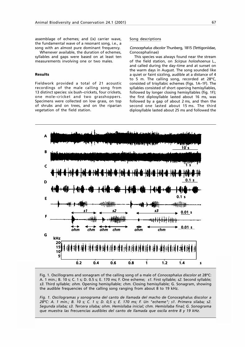
Animal Biodiversity and Conservation 24.1 (2001) 67
assemblage of echemes; and (ix) carrier wave,the fundamental wave of a resonant song, i.e., asong with an almost pure dominant frequency.
Whenever available, the duration of echemes,syllables and gaps were based on at least tenmeasurements involving one or two males.
Results
Fieldwork provided a total of 21 acousticrecordings of the male calling song from13 distinct species: six bush–crickets, four crickets,one mole–cricket and two grasshoppers.Specimens were collected on low grass, on topof shrubs and on trees, and on the riparianvegetation of the field station.
Song descriptions
Conocephalus discolor Thunberg, 1815 (Tettigoniidae,Conocephalinae)
This species was always found near the streamof the field station, on Scirpus holoshoenus L.,and called during the day–time and at sunset onthe warm days in August. The song sounded likea quiet or faint sizzling, audible at a distance of 4to 5 m. The calling song, recorded at 28ºC,consisted of trisyllabic echemes (figs. 1A–1F). Thesyllables consisted of short opening hemisyllables,followed by longer closing hemisyllables (fig. 1F);the first diplosyllable lasted about 16 ms, wasfollowed by a gap of about 2 ms, and then thesecond one lasted about 15 ms. The thirddiplosyllable lasted about 25 ms and followed the
Fig. 1. Oscillograms and sonagram of the calling song of a male of Conocephalus discolor at 28ºC:A. 1 min.; B. 10 s; C. 1 s; D. 0.5 s; E. 170 ms; F. One echeme; s1. First syllable; s2. Second syllable;s3. Third syllable; ohm. Opening hemisyllable; chm. Closing hemisyllable; G. Sonagram, showingthe audible frequencies of the calling song ranging from about 8 to 19 kHz.
Fig. 1. Oscilogramas y sonograma del canto de llamada del macho de Conocephalus discolor a28ºC: A. 1 min.; B. 10 s; C. 1 s; D. 0,5 s; E. 170 ms; F. Un "echeme"; s1. Primera sílaba; s2.Segunda sílaba; s3. Tercera sílaba; ohm. Hemisílaba inicial; chm. Hemisílaba final; G. Sonogramaque muestra las frecuencias audibles del canto de llamada que oscila entre 8 y 19 kHz.
AAAAA
BBBBB
CCCCC
DDDDD
EEEEE
FFFFF
GGGGG
1 s1 s1 s1 s1 s
0.01 s0.01 s0.01 s0.01 s0.01 s s1 s1 s1 s1 s1 s2 s2 s2 s2 s2 s3 s3 s3 s3 s3
ohm chm ohm chmohm chm ohm chmohm chm ohm chmohm chm ohm chmohm chm ohm chm ohm ohm ohm ohm ohm chm chm chm chm chm0.01 s0.01 s0.01 s0.01 s0.01 s
kHzkHzkHzkHzkHz202020202015151515151010101010
55555
0.2 0.2 0.2 0.2 0.2 0.4 0.4 0.4 0.4 0.4 0.6 0.6 0.6 0.6 0.6 0.8 0.8 0.8 0.8 0.8 1 1 1 1 1 1.2 1.2 1.2 1.2 1.2 1.4 1.4 1.4 1.4 1.4 s s s s s
10 s10 s10 s10 s10 s
0.1 s0.1 s0.1 s0.1 s0.1 s
0.1 s0.1 s0.1 s0.1 s0.1 s
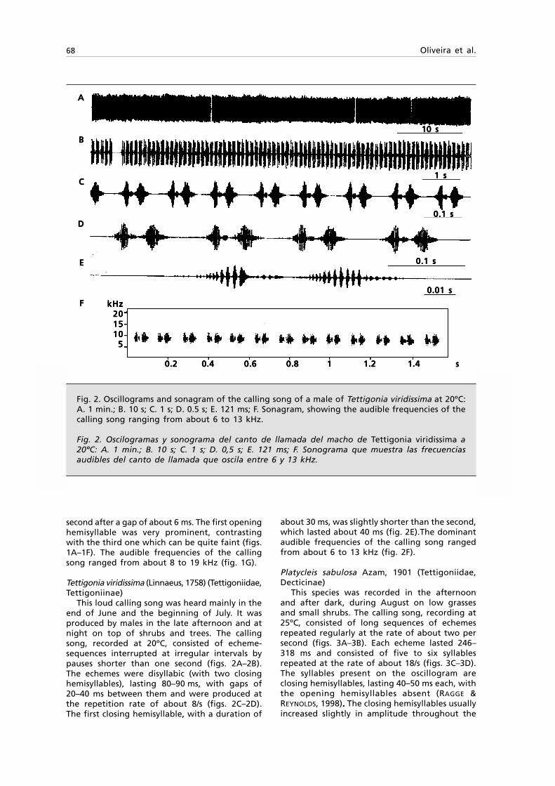
68 Oliveira et al.
Fig. 2. Oscillograms and sonagram of the calling song of a male of Tettigonia viridissima at 20ºC:A. 1 min.; B. 10 s; C. 1 s; D. 0.5 s; E. 121 ms; F. Sonagram, showing the audible frequencies of thecalling song ranging from about 6 to 13 kHz.
Fig. 2. Oscilogramas y sonograma del canto de llamada del macho de Tettigonia viridissima a20ºC: A. 1 min.; B. 10 s; C. 1 s; D. 0,5 s; E. 121 ms; F. Sonograma que muestra las frecuenciasaudibles del canto de llamada que oscila entre 6 y 13 kHz.
second after a gap of about 6 ms. The first openinghemisyllable was very prominent, contrastingwith the third one which can be quite faint (figs.1A–1F). The audible frequencies of the callingsong ranged from about 8 to 19 kHz (fig. 1G).
Tettigonia viridissima (Linnaeus, 1758) (Tettigoniidae,Tettigoniinae)
This loud calling song was heard mainly in theend of June and the beginning of July. It wasproduced by males in the late afternoon and atnight on top of shrubs and trees. The callingsong, recorded at 20ºC, consisted of echeme-sequences interrupted at irregular intervals bypauses shorter than one second (figs. 2A–2B).The echemes were disyllabic (with two closinghemisyllables), lasting 80–90 ms, with gaps of20–40 ms between them and were produced atthe repetition rate of about 8/s (figs. 2C–2D).The first closing hemisyllable, with a duration of
about 30 ms, was slightly shorter than the second,which lasted about 40 ms (fig. 2E).The dominantaudible frequencies of the calling song rangedfrom about 6 to 13 kHz (fig. 2F).
Platycleis sabulosa Azam, 1901 (Tettigoniidae,Decticinae)
This species was recorded in the afternoonand after dark, during August on low grassesand small shrubs. The calling song, recording at25ºC, consisted of long sequences of echemesrepeated regularly at the rate of about two persecond (figs. 3A–3B). Each echeme lasted 246–318 ms and consisted of five to six syllablesrepeated at the rate of about 18/s (figs. 3C–3D).The syllables present on the oscillogram areclosing hemisyllables, lasting 40–50 ms each, withthe opening hemisyllables absent (RAGGE &REYNOLDS, 1998)..... The closing hemisyllables usuallyincreased slightly in amplitude throughout the
AAAAA
BBBBB
CCCCC
DDDDD
EEEEE
FFFFF kHzkHzkHzkHzkHz202020202015151515151010101010
55555
0.2 0.2 0.2 0.2 0.2 0.4 0.4 0.4 0.4 0.4 0.6 0.6 0.6 0.6 0.6 0.8 1 1.2 1.40.8 1 1.2 1.40.8 1 1.2 1.40.8 1 1.2 1.40.8 1 1.2 1.4 s s s s s
10 s10 s10 s10 s10 s
1 s1 s1 s1 s1 s
0.1 s0.1 s0.1 s0.1 s0.1 s
0.1 s0.1 s0.1 s0.1 s0.1 s
0.01 s0.01 s0.01 s0.01 s0.01 s

Animal Biodiversity and Conservation 24.1 (2001) 69
Fig. 3. Oscillograms and sonagram of the calling song of a male of Platycleis sabulosa at 25ºC:A. 1 min.; B. 10 s; C. 2.3 s; D. 1 s; E. Sonagram, showing the audible frequencies of the callingsong ranging from about 6 to 19 kHz.
Fig. 3. Oscilogramas y sonograma del canto de llamada del macho de Platycleis sabulosa a 25ºC:A. 1 min.; B. 10 s; C. 2,3 s; D. 1 s; E. Sonograma que muestra las frecuencias audibles del cantode llamada que oscila entre 6 y 19 kHz.
echeme (figs. 3A–3D), appearing slightly longerthan those given by RAGGE & REYNOLDS (1998).The audible frequencies of the calling songranged from about 6 to 19 kHz (fig. 3E).This is anew record for Portugal.
Platycleis affinis Fieber, 1853 (Tettigoniidae,Decticinae)
This species was found on low grass, in theevening and early at night in August. The callingsong, recorded at 28ºC, consisted of a typical mixtureof short echemes (figs. 4C–4F), lasting less than onesecond and usually composed of three to fourmacrosyllables, and longer echemes (figs. 4C–4D)lasting from four to eight seconds and composed of33–53 macrosyllables; these latter, therefore, slightlylonger than those given by RAGGE & REYNOLDS (1998).Each echeme usually ends with a series of 7–10microsyllables. The echemes are often grouped intotwo to five short ones followed by a long one (fig.4A–4B). Macrosyllables are repeated at the rate of
about eight per second and microsyllables at about21/s. Similarly to P. sabulosa, the audible frequenciesof the calling song ranged from about 7 to 19 kHz(fig. 4G).
Platycleis intermedia (Serville, 1838) (Tettigoniidae,Decticinae)
This bush–cricket called on low grasses and onsmall shrubs mostly in the late evening and atnight in August and September. The calling song,recorded at 28ºC, consisted of long sequences ofdisyllabic echemes, consisting of two closinghemisyllables, and repeated at the rate of aboutthree per second (figs. 5A–5B); the duration ofeach echeme varied between 150 and 160 ms andthe gap between consecutive echemes variedbetween 160 and 180 ms. The second closinghemisyllable of each pair was slightly longer andlouder than the first (figs. 5C–5D). As with the twoprevious species, the audible frequencies of the callingsong ranged from about 6 to 19 kHz (fig. 5E).
AAAAA
BBBBB
CCCCC
DDDDD
EEEEEkHzkHzkHzkHzkHz
202020202015151515151010101010
55555
0.2 0.2 0.2 0.2 0.2 0.4 0.4 0.4 0.4 0.4 0.6 0.6 0.6 0.6 0.6 0.80.80.80.80.8 1 1 1 1 1 1.2 1.4 1.2 1.4 1.2 1.4 1.2 1.4 1.2 1.4 1.6 1.6 1.6 1.6 1.6 1.8 2 1.8 2 1.8 2 1.8 2 1.8 2 s s s s s
10 s10 s10 s10 s10 s
1 s1 s1 s1 s1 s
0.5 s0.5 s0.5 s0.5 s0.5 s
0.1 s0.1 s0.1 s0.1 s0.1 s
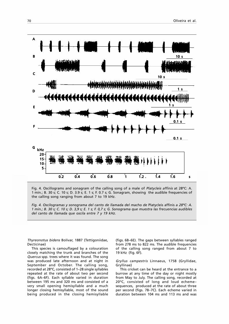
70 Oliveira et al.
Fig. 4. Oscillograms and sonagram of the calling song of a male of Platycleis affinis at 28ºC: A.1 min.; B. 30 s; C. 10 s; D. 3.9 s; E. 1 s; F. 0.7 s; G. Sonagram, showing the audible frequencies ofthe calling song ranging from about 7 to 19 kHz.
Fig. 4. Oscilogramas y sonograma del canto de llamada del macho de Platycleis affinis a 28ºC: A.1 min.; B. 30 s; C. 10 s; D. 3,9 s; E. 1 s; F. 0,7 s; G. Sonograma que muestra las frecuencias audiblesdel canto de llamada que oscila entre 7 y 19 kHz.
Thyreonotus bidens Bolívar, 1887 (Tettigoniidae,Decticinae)
This species is camouflaged by a colourationclosely matching the trunk and branches of theQuercus spp. trees where it was found. The songwas produced late afternoon and at night inSeptember and October. The calling song,recorded at 28ºC, consisted of 1–28 single syllablesrepeated at the rate of about two per second(figs. 6A–6F). Each syllable varied in durationbetween 195 ms and 320 ms and consisted of avery small opening hemisyllable and a muchlonger closing hemisyllable, most of the soundbeing produced in the closing hemisyllable
(figs. 6B–6E). The gaps between syllables rangedfrom 278 ms to 822 ms. The audible frequenciesof the calling song ranged from about 7 to19 kHz (fig. 6F).
Gryllus campestris Linnaeus, 1758 (Gryllidae,Gryllinae)
This cricket can be heard at the entrance to aburrow at any time of the day or night mostlyfrom May to July. The calling song, recorded at20ºC, consisted of long and loud echeme–sequences, produced at the rate of about threeper second (figs. 7B–7C). Each echeme varied induration between 104 ms and 113 ms and was
AAAAA
BBBBB
CCCCC
DDDDD
EEEEE
FFFFF
GGGGGkHzkHzkHzkHzkHz
202020202015151515151010101010
55555
0.2 0.2 0.2 0.2 0.2 0.4 0.4 0.4 0.4 0.4 0.60.60.60.60.6 0.8 0.8 0.8 0.8 0.8 1 1 1 1 1 1.2 1.2 1.2 1.2 1.2 . 1.4. 1.4. 1.4. 1.4. 1.4 1.6 1.6 1.6 1.6 1.6 sssss
10 s10 s10 s10 s10 s
10 s10 s10 s10 s10 s
1 s1 s1 s1 s1 s
0.1 s0.1 s0.1 s0.1 s0.1 s
0.1 s0.1 s0.1 s0.1 s0.1 s
1 s1 s1 s1 s1 s
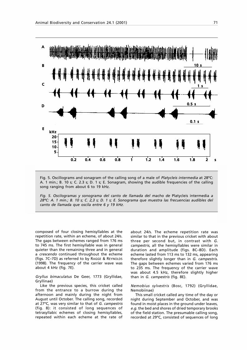
Animal Biodiversity and Conservation 24.1 (2001) 71
Fig. 5. Oscillograms and sonagram of the calling song of a male of Platycleis intermedia at 28ºC:A. 1 min.; B. 10 s; C. 2.3 s; D. 1 s; E. Sonagram, showing the audible frequencies of the callingsong ranging from about 6 to 19 kHz.
Fig. 5. Oscilogramas y sonograma del canto de llamada del macho de Platycleis intermedia a28ºC: A. 1 min.; B. 10 s; C. 2,3 s; D. 1 s; E. Sonograma que muestra las frecuencias audibles delcanto de llamada que oscila entre 6 y 19 kHz.
composed of four closing hemisyllables at therepetition rate, within an echeme, of about 24/s.The gaps between echemes ranged from 176 msto 745 ms. The first hemisyllable was in generalquieter than the remaining three and in generala crescendo continued throughout the echeme(figs. 7C–7D) as referred to by RAGGE & REYNOLDS
(1998). The frequency of the carrier wave wasabout 4 kHz (fig. 7E).
Gryllus bimaculatus De Geer, 1773 (Gryllidae,Gryllinae)
Like the previous species, this cricket calledfrom the entrance to a burrow during theafternoon and mainly during the night fromAugust until October. The calling song, recordedat 27ºC, was very similar to that of G. campestris(fig. 8): it consisted of long sequences oftetrasyllabic echemes of closing hemisyllables,repeated within each echeme at the rate of
about 24/s. The echeme repetition rate wassimilar to that in the previous cricket with aboutthree per second but, in contrast with G.campestris, all the hemisyllables were similar induration and amplitude (figs. 8C–8D). Eachecheme lasted from 113 ms to 132 ms, appearingtherefore slightly longer than in G. campestris.The gaps between echemes varied from 176 msto 235 ms. The frequency of the carrier wavewas about 4.5 kHz, therefore slightly higherthan in G. campestris (fig. 8E).
Nemobius sylvestris (Bosc, 1792) (Gryllidae,Nemobiinae)
This small cricket called any time of the day ornight during September and October, and wasfound in moist places in the ground under leaves,e.g. the bed and shores of dried temporary brooksof the field station. The presumable calling song,recorded at 29ºC, consisted of sequences of long
AAAAA
BBBBB
CCCCC
DDDDD
EEEEEkHzkHzkHzkHzkHz
202020202015151515151010101010
55555
0.2 0.2 0.2 0.2 0.2 0.4 0.4 0.4 0.4 0.4 0.6 0.8 0.6 0.8 0.6 0.8 0.6 0.8 0.6 0.8 1 1 1 1 1 1.2 1.2 1.2 1.2 1.2 1.4 1.6 1.4 1.6 1.4 1.6 1.4 1.6 1.4 1.6 1.8 1.8 1.8 1.8 1.8 2 2 2 2 2 s s s s s
10 s10 s10 s10 s10 s
1 s1 s1 s1 s1 s
0.5 s0.5 s0.5 s0.5 s0.5 s
0.1 s0.1 s0.1 s0.1 s0.1 s

72 Oliveira et al.
Fig. 6. Oscillograms and sonagram of the calling song of a male of Thyreonotus bidens at 28ºC:A. 1 min.; B. 10 s; C. 2.3 s; D. 1 s; E. 0.5 s; F. Sonagram, showing the audible frequencies of thecalling song ranging from about 7 to 19 kHz.
Fig. 6. Oscilogramas y sonograma del canto de llamada del macho de Thyreonotus bidens a 28ºC:A. 1 min.; B. 10 s; C. 2,3 s; D. 1 s; E. 0,5 s; F. Sonograma que muestra las frecuencias audibles delcanto de llamada que oscila entre 7 y 19 kHz.
echemes repeated at the rate of about 0.5/s(figs. 9A–9B). The duration of each echemedepended on the number of syllables, whichwere between 12 and 62 (fig. 9C), thereforeconsiderably longer than those described byRAGGE & REYNOLDS (1998). It is possible that thisatypical sound might represent instead acourtship sound. The syllables were repeated atthe rate of about 32/s, lasting about 9 ms eachand with a gap of 15 to 20 ms between them.The first 8–12 syllables showed an increase inamplitude (figs. 9C–9D). The frequency of thecarrier wave was about 3.8 kHz (fig. 9E).
Oecanthus pellucens (Scopoli, 1763) (Gryllidae,Oecanthinae)
This slender and yellowish cricket called on topof low grass or on small bushes in July and August.
The calling song, recorded at 22ºC, consisted oflong echemesequences (figs. 10A–10B). Theduration of each echeme varied between 800 and1300 ms, at a repetition rate of about 0.6/s, andthe gap between consecutive echemes varied from400 to 500 ms. Each echeme was composed of 18–29 syllables at the repetition rate of about 22/s(figs. 10C–10D). Each syllable lasted about 32 msand the gap between successive syllables wasabout 10 ms. The frequency of the carrier wavewas about 2.3 kHz (fig. 10E).
Gryllotalpa vineae Bennet–Clark, 1970 (Gryllotalpidae,Gryllotalpinae)
Like most mole–crickets, this species producesits song from a specially made singing burrow,with a pair of short horn–shaped passages,leading to two entrance holes. The song is very
AAAAA
BBBBB
CCCCC
DDDDD
EEEEE
FFFFF
10 s10 s10 s10 s10 s
1 s1 s1 s1 s1 s
0.5 s0.5 s0.5 s0.5 s0.5 s
0.1 s0.1 s0.1 s0.1 s0.1 s
0.1 s0.1 s0.1 s0.1 s0.1 s
kHzkHzkHzkHzkHz
2020202020
1515151515
1010101010
55555
0.2 0.2 0.2 0.2 0.2 0.4 0.4 0.4 0.4 0.4 0.6 0.6 0.6 0.6 0.6 0.80.80.80.80.8 1 1 1 1 1 1.2 1.4 1.2 1.4 1.2 1.4 1.2 1.4 1.2 1.4 1.61.61.61.61.6 1.8 1.8 1.8 1.8 1.8 2 2 2 2 2 s s s s s
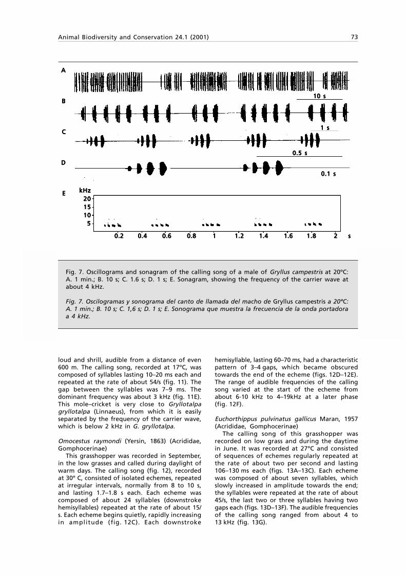
Animal Biodiversity and Conservation 24.1 (2001) 73
Fig. 7. Oscillograms and sonagram of the calling song of a male of Gryllus campestris at 20ºC:A. 1 min.; B. 10 s; C. 1.6 s; D. 1 s; E. Sonagram, showing the frequency of the carrier wave atabout 4 kHz.
Fig. 7. Oscilogramas y sonograma del canto de llamada del macho de Gryllus campestris a 20ºC:A. 1 min.; B. 10 s; C. 1,6 s; D. 1 s; E. Sonograma que muestra la frecuencia de la onda portadoraa 4 kHz.
loud and shrill, audible from a distance of even600 m. The calling song, recorded at 17ºC, wascomposed of syllables lasting 10–20 ms each andrepeated at the rate of about 54/s (fig. 11). Thegap between the syllables was 7–9 ms. Thedominant frequency was about 3 kHz (fig. 11E).This mole–cricket is very close to Gryllotalpagryllotalpa (Linnaeus), from which it is easilyseparated by the frequency of the carrier wave,which is below 2 kHz in G. gryllotalpa.
Omocestus raymondi (Yersin, 1863) (Acrididae,Gomphocerinae)
This grasshopper was recorded in September,in the low grasses and called during daylight ofwarm days. The calling song (fig. 12), recordedat 30º C, consisted of isolated echemes, repeatedat irregular intervals, normally from 8 to 10 s,and lasting 1.7–1.8 s each. Each echeme wascomposed of about 24 syllables (downstrokehemisyllables) repeated at the rate of about 15/s. Each echeme begins quietly, rapidly increasingin amplitude (fig. 12C). Each downstroke
hemisyllable, lasting 60–70 ms, had a characteristicpattern of 3–4 gaps, which became obscuredtowards the end of the echeme (figs. 12D–12E).The range of audible frequencies of the callingsong varied at the start of the echeme fromabout 6-10 kHz to 4–19kHz at a later phase(fig. 12F).
Euchorthippus pulvinatus gallicus Maran, 1957(Acrididae, Gomphocerinae)
The calling song of this grasshopper wasrecorded on low grass and during the daytimein June. It was recorded at 27ºC and consistedof sequences of echemes regularly repeated atthe rate of about two per second and lasting106–130 ms each (figs. 13A–13C). Each echemewas composed of about seven syllables, whichslowly increased in amplitude towards the end;the syllables were repeated at the rate of about45/s, the last two or three syllables having twogaps each (figs. 13D–13F). The audible frequenciesof the calling song ranged from about 4 to13 kHz (fig. 13G).
AAAAA
BBBBB
CCCCC
DDDDD
EEEEE kHzkHzkHzkHzkHz202020202015151515151010101010
55555
0.2 0.2 0.2 0.2 0.2 0.4 0.4 0.4 0.4 0.4 0.6 0.8 0.6 0.8 0.6 0.8 0.6 0.8 0.6 0.8 1 1 1 1 1 1.2 1.2 1.2 1.2 1.2 1.4 1.6 1.4 1.6 1.4 1.6 1.4 1.6 1.4 1.6 1.81.81.81.81.8 2 2 2 2 2 s s s s s
10 s10 s10 s10 s10 s
1 s1 s1 s1 s1 s
0.5 s0.5 s0.5 s0.5 s0.5 s
0.1 s0.1 s0.1 s0.1 s0.1 s

74 Oliveira et al.
Fig. 8. Oscillograms and sonagram of the calling song of a male of Gryllus bimaculatus at 27ºC: A.1 min; B. 10 s; C. 1.6 s; D. 1 s; E. Sonagram, showing the frequency of the carrier wave at about 4.5 kHz.
Fig. 8. Oscilogramas y sonograma del canto de llamada del macho de Gryllus bimaculatus a 27ºC: A.1 min; B. 10 s; C. 1,6 s; D. 1 s; E. Sonograma que muestra la frecuencia de la onda portadora a 4,5 kHz.
Fig. 9. Oscillograms and sonagram of the calling song of a male of Nemobius sylvestris at 29ºC: A.1 min.; B. 10 s; C. 2.4 s; D. 1 s; E. Sonagram, showing the frequency of the carrier wave at about 3.8 kHz.
Fig. 9. Oscilogramas y sonograma del canto de llamada del macho de Nemobius sylvestris a 29ºC: A.1 min.; B. 10 s; C. 2,4 s; D. 1 s; E. Sonograma que muestra la frecuencia de la onda portadora a 3,8 kHz.
AAAAA
BBBBB
CCCCC
DDDDD
EEEEE
AAAAA
BBBBB
CCCCC
DDDDD
EEEEE
1 s1 s1 s1 s1 s
1 s1 s1 s1 s1 s
10 s10 s10 s10 s10 s
10 s10 s10 s10 s10 s
0.5 s0.5 s0.5 s0.5 s0.5 s
0.1 s0.1 s0.1 s0.1 s0.1 s
kHzkHzkHzkHzkHz202020202015151515151010101010
55555
0.2 0.4 0.6 0.2 0.4 0.6 0.2 0.4 0.6 0.2 0.4 0.6 0.2 0.4 0.6 0.8 0.8 0.8 0.8 0.8 1 1 1 1 1 1.2 1.2 1.2 1.2 1.2 1.4 1.4 1.4 1.4 1.4 1.6 1.6 1.6 1.6 1.6 1.8 2 1.8 2 1.8 2 1.8 2 1.8 2 s s s s s
0.5 s0.5 s0.5 s0.5 s0.5 s
kHzkHzkHzkHzkHz202020202015151515151010101010
55555
0.2 0.4 0.6 0.8 1 0.2 0.4 0.6 0.8 1 0.2 0.4 0.6 0.8 1 0.2 0.4 0.6 0.8 1 0.2 0.4 0.6 0.8 1 1.2 1.2 1.2 1.2 1.2 1.4 1.4 1.4 1.4 1.4 1.6 1.6 1.6 1.6 1.6 1.8 1.8 1.8 1.8 1.8 2 2 2 2 2 s s s s s
0.1 s0.1 s0.1 s0.1 s0.1 s
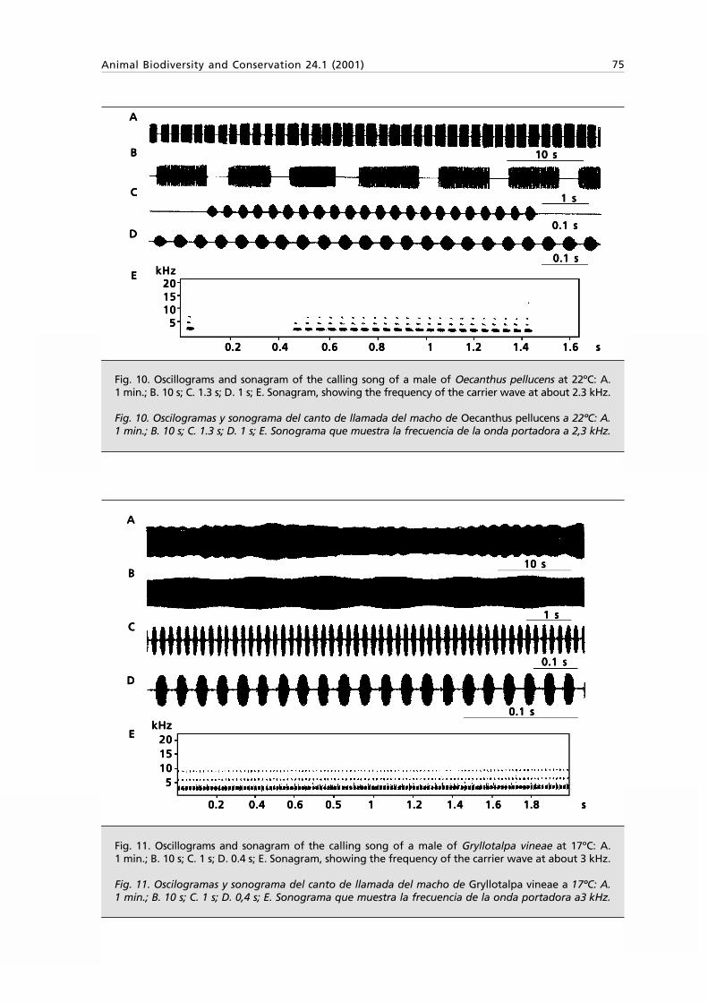
Animal Biodiversity and Conservation 24.1 (2001) 75
Fig. 10. Oscillograms and sonagram of the calling song of a male of Oecanthus pellucens at 22ºC: A.1 min.; B. 10 s; C. 1.3 s; D. 1 s; E. Sonagram, showing the frequency of the carrier wave at about 2.3 kHz.
Fig. 10. Oscilogramas y sonograma del canto de llamada del macho de Oecanthus pellucens a 22ºC: A.1 min.; B. 10 s; C. 1.3 s; D. 1 s; E. Sonograma que muestra la frecuencia de la onda portadora a 2,3 kHz.
Fig. 11. Oscillograms and sonagram of the calling song of a male of Gryllotalpa vineae at 17ºC: A.1 min.; B. 10 s; C. 1 s; D. 0.4 s; E. Sonagram, showing the frequency of the carrier wave at about 3 kHz.
Fig. 11. Oscilogramas y sonograma del canto de llamada del macho de Gryllotalpa vineae a 17ºC: A.1 min.; B. 10 s; C. 1 s; D. 0,4 s; E. Sonograma que muestra la frecuencia de la onda portadora a3 kHz.
AAAAA
BBBBB
CCCCC
DDDDD
EEEEE
AAAAA
BBBBB
CCCCC
DDDDD
EEEEE
10 s10 s10 s10 s10 s
10 s10 s10 s10 s10 s
1 s1 s1 s1 s1 s
0.1 s0.1 s0.1 s0.1 s0.1 s
1 s1 s1 s1 s1 s
0.1 s0.1 s0.1 s0.1 s0.1 s
0.1 s0.1 s0.1 s0.1 s0.1 skHzkHzkHzkHzkHz
202020202015151515151010101010
55555
0.2 0.2 0.2 0.2 0.2 0.4 0.4 0.4 0.4 0.4 0.6 0.6 0.6 0.6 0.6 0.5 0.5 0.5 0.5 0.5 1 1 1 1 1 1.2 1.2 1.2 1.2 1.2 1.41.41.41.41.4 1.6 1.6 1.6 1.6 1.6 1.8 1.8 1.8 1.8 1.8 sssss
0.1 s0.1 s0.1 s0.1 s0.1 s
kHzkHzkHzkHzkHz202020202015151515151010101010
55555
0.2 0.2 0.2 0.2 0.2 0.4 0.4 0.4 0.4 0.4 0.6 0.6 0.6 0.6 0.6 0.8 0.8 0.8 0.8 0.8 1 1 1 1 1 1.2 1.2 1.2 1.2 1.2 1.4 1.4 1.4 1.4 1.4 1.6 1.6 1.6 1.6 1.6 s s s s s
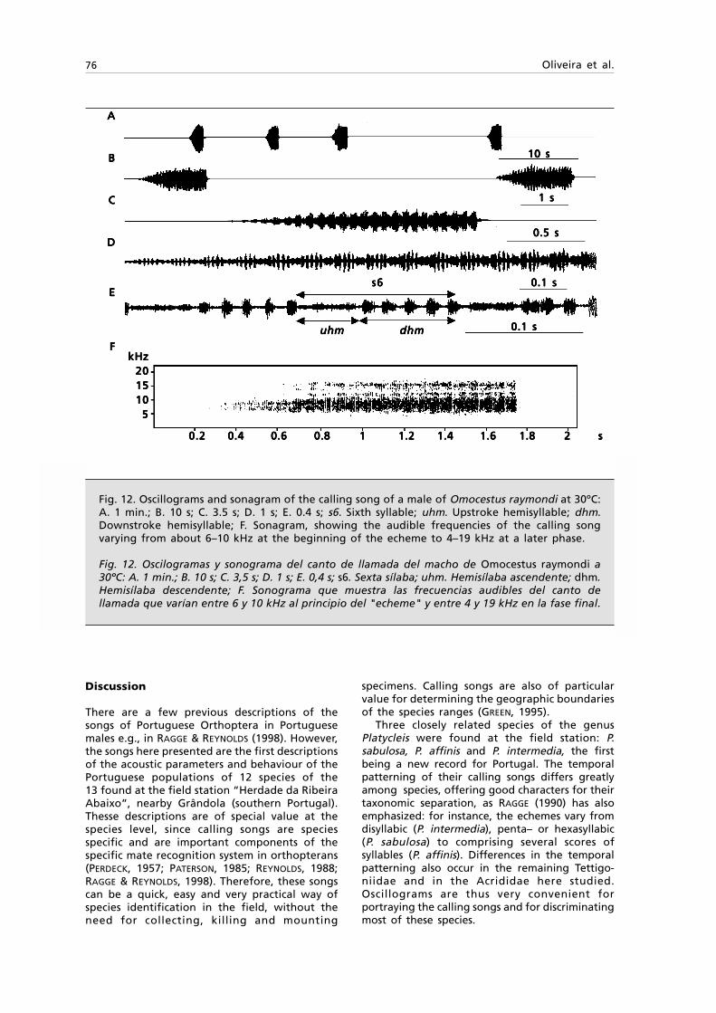
76 Oliveira et al.
Discussion
There are a few previous descriptions of thesongs of Portuguese Orthoptera in Portuguesemales e.g., in RAGGE & REYNOLDS (1998). However,the songs here presented are the first descriptionsof the acoustic parameters and behaviour of thePortuguese populations of 12 species of the13 found at the field station “Herdade da RibeiraAbaixo”, nearby Grândola (southern Portugal).Thesse descriptions are of special value at thespecies level, since calling songs are speciesspecific and are important components of thespecific mate recognition system in orthopterans(PERDECK, 1957; PATERSON, 1985; REYNOLDS, 1988;RAGGE & REYNOLDS, 1998). Therefore, these songscan be a quick, easy and very practical way ofspecies identification in the field, without theneed for collecting, killing and mounting
specimens. Calling songs are also of particularvalue for determining the geographic boundariesof the species ranges (GREEN, 1995).
Three closely related species of the genusPlatycleis were found at the field station: P.sabulosa, P. affinis and P. intermedia, the firstbeing a new record for Portugal. The temporalpatterning of their calling songs differs greatlyamong species, offering good characters for theirtaxonomic separation, as RAGGE (1990) has alsoemphasized: for instance, the echemes vary fromdisyllabic (P. intermedia), penta– or hexasyllabic(P. sabulosa) to comprising several scores ofsyllables (P. affinis). Differences in the temporalpatterning also occur in the remaining Tettigo-niidae and in the Acrididae here studied.Oscillograms are thus very convenient forportraying the calling songs and for discriminatingmost of these species.
Fig. 12. Oscillograms and sonagram of the calling song of a male of Omocestus raymondi at 30ºC:A. 1 min.; B. 10 s; C. 3.5 s; D. 1 s; E. 0.4 s; s6. Sixth syllable; uhm. Upstroke hemisyllable; dhm.Downstroke hemisyllable; F. Sonagram, showing the audible frequencies of the calling songvarying from about 6–10 kHz at the beginning of the echeme to 4–19 kHz at a later phase.
Fig. 12. Oscilogramas y sonograma del canto de llamada del macho de Omocestus raymondi a30ºC: A. 1 min.; B. 10 s; C. 3,5 s; D. 1 s; E. 0,4 s; s6. Sexta sílaba; uhm. Hemisílaba ascendente; dhm.Hemisílaba descendente; F. Sonograma que muestra las frecuencias audibles del canto dellamada que varían entre 6 y 10 kHz al principio del "echeme" y entre 4 y 19 kHz en la fase final.
AAAAA
BBBBB
CCCCC
DDDDD
EEEEE
FFFFF
10 s10 s10 s10 s10 s
1 s1 s1 s1 s1 s
0.1 s0.1 s0.1 s0.1 s0.1 s
uhmuhmuhmuhmuhm dhmdhmdhmdhmdhm
s6s6s6s6s6
0.1 s0.1 s0.1 s0.1 s0.1 s
kHzkHzkHzkHzkHz202020202015151515151010101010
55555
0.20.20.20.20.2 0.4 0.4 0.4 0.4 0.4 0.6 0.6 0.6 0.6 0.6 0.8 0.8 0.8 0.8 0.8 11111 1.2 1.2 1.2 1.2 1.2 1.4 1.4 1.4 1.4 1.4 1.6 1.8 1.6 1.8 1.6 1.8 1.6 1.8 1.6 1.8 22222 sssss
0.5 s0.5 s0.5 s0.5 s0.5 s
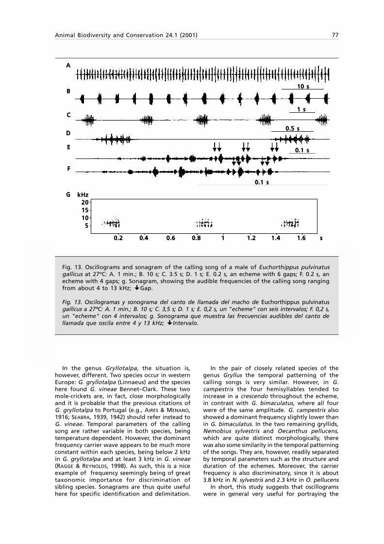
Animal Biodiversity and Conservation 24.1 (2001) 77
In the genus Gryllotalpa, the situation is,however, different. Two species occur in westernEurope: G. gryllotalpa (Linnaeus) and the specieshere found G. vineae Bennet–Clark. These twomole-crickets are, in fact, close morphologicallyand it is probable that the previous citations ofG. gryllotalpa to Portugal (e.g., AIRES & MENANO,1916; SEABRA, 1939, 1942) should refer instead toG. vineae. Temporal parameters of the callingsong are rather variable in both species, beingtemperature dependent. However, the dominantfrequency carrier wave appears to be much moreconstant within each species, being below 2 kHzin G. gryllotalpa and at least 3 kHz in G. vineae(RAGGE & REYNOLDS, 1998). As such, this is a niceexample of frequency seemingly being of greattaxonomic importance for discrimination ofsibling species. Sonagrams are thus quite usefulhere for specific identification and delimitation.
In the pair of closely related species of thegenus Gryllus the temporal patterning of thecalling songs is very similar. However, in G.campestris the four hemisyllables tended toincrease in a crescendo throughout the echeme,in contrast with G. bimaculatus, where all fourwere of the same amplitude. G. campestris alsoshowed a dominant frequency slightly lower thanin G. bimaculatus. In the two remaining gryllids,Nemobius sylvestris and Oecanthus pellucens,which are quite distinct morphologically, therewas also some similarity in the temporal patterningof the songs. They are, however, readily separatedby temporal parameters such as the structure andduration of the echemes. Moreover, the carrierfrequency is also discriminatory, since it is about3.8 kHz in N. sylvestris and 2.3 kHz in O. pellucens
In short, this study suggests that oscillogramswere in general very useful for portraying the
Fig. 13. Oscillograms and sonagram of the calling song of a male of Euchorthippus pulvinatusgallicus at 27ºC: A. 1 min.; B. 10 s; C. 3.5 s; D. 1 s; E. 0.2 s, an echeme with 6 gaps; F. 0.2 s, anecheme with 4 gaps; g. Sonagram, showing the audible frequencies of the calling song rangingfrom about 4 to 13 kHz; �Gap.
Fig. 13. Oscilogramas y sonograma del canto de llamada del macho de Euchorthippus pulvinatusgallicus a 27ºC: A. 1 min.; B. 10 s; C. 3,5 s; D. 1 s; E. 0,2 s, un "echeme" con seis intervalos; F. 0,2 s,un "echeme" con 4 intervalos; g. Sonograma que muestra las frecuencias audibles del canto dellamada que oscila entre 4 y 13 kHz; �Intervalo.
1 s1 s1 s1 s1 s
10 s10 s10 s10 s10 s
AAAAA
BBBBB
CCCCC
DDDDD
EEEEE
FFFFF
GGGGG kHzkHzkHzkHzkHz202020202015151515151010101010
55555
0.2 0.2 0.2 0.2 0.2 0.4 0.4 0.4 0.4 0.4 0.6 0.6 0.6 0.6 0.6 0.8 0.8 0.8 0.8 0.8 1 1 1 1 1 1.2 1.2 1.2 1.2 1.2 1.41.41.41.41.4 1.6 1.6 1.6 1.6 1.6 s s s s s
0.5 s0.5 s0.5 s0.5 s0.5 s
0.1 s0.1 s0.1 s0.1 s0.1 s
0.1 s0.1 s0.1 s0.1 s0.1 s
78 Oliveira et al.
calling songs of the species here studied. On theother hand, except for Gryllidae and Gryllotal-pidae, sonagrams from audio recordings may givea misleading impression of the frequency spectrumof the song, which in Acrididae and Tettigoniidaeextends well into the ultrasonic range, and insome Tettigonniidae is mainly ultrasonic. ForGryllidae and Gryllotalpidae, the carrier frequencycan be measured more accurately from fastoscillograms than from sonagrams (D. R. Ragge,pers. comm.). Nevertheless, sonagrams are a usefuladdition to song analysis, especially if they includethe full frequency spectrum of the song. Therefore,the simultaneous use of both oscillograms andsonagrams is encouraged.
Finally, as previously mentioned, one speciesfound at the field station —Platycleis sabulosaAzam—, is here recorded for the first time fromPortugal. Moreover, considering the smallgeographic area investigated many more newrecords are yet to be found in this country andhence further studies dealing with these insectsshould be encouraged.
Acknowledgements
For their help in the field work, as well as forother support the authors would like to expresstheir sincere thanks to Dr. Arabolaza (EscolaSuperior Agrária, Bragança), Dr. Bívar de Sousa(Sociedade Portuguesa de Entomologia, Lisboa),and Mr. Genage André (Departamento deZoologia e Antropologia, Faculdade de Ciências,Universidade de Lisboa). Finally, the authorsgreatly appreciate the comments of Dr. D. R.Ragge, who kindly accepted to critically readingthe manuscript.
References
AIRES, B. & MENANO, H. P., 1916. Catálogo sinópticodos ortópteros de Portugal. Univ. de Coimbra,Coimbra.
ALEXANDER, R. D., 1968. Arthropods. In: AnimalCommunication: Techniques of Study andResults of Research: 167–216 (T. A. Sebeok,Ed.). Indiana University Press, Bloomington.
CHAPMAN, R. F., 2000. The Insects. Structure andFunction, 4th edition. Cambridge UniversityPress, Cambridge.
CLARIDGE, M. F., 1985. Acoustic signals in theHomoptera: behaviour, taxonomy and evolution.Annual Review of Entomology, 30: 297–317.
DUMORTIER, B., 1963. Ethological and physiologicalstudy of sound emission in Arthropods. In:Acoustic Behaviour of Animals: 583–684 (R. G.Busnel, Ed.). Elsevier Pub. Co., Amsterdam.
ELSNER, N., 1983. Insect stridulation and itsneurophysiological basis. In: Bioacoustics, acomparative approach: 69–92 (B. Lewis, Ed.).Academic Press, London.
EWING, A. W., 1984. Acoustic signals in insectsexual behaviour. In: Insect communication:223–240 (T. Lewis, Ed.). Academic Press, London.
GREEN, S. V., 1995. Song characteristics of certainNamibian grasshoppers (Orthoptera: Acrididae:Gomphocerinae). African Entomology, 33333(1): 1–6.
HASKELL, P. T., 1974. Sound Production. In: Thephysiology of Insecta., vol. 2: 354–410 (M.Rockstein, Ed.). Academic Press, New York andLondon.
OTTE, D., 1977. Communication in Orthoptera.In: How Animals Communicate, Part. I: 334–361 (T. A. Sebeok, Ed.). Indiana UniversityPress, Bloomington and London.
PATERSON, H. E. H., 1985. The recognition conceptsof species. In: Species and Speciation: 21–29(E. S. Vrba, Ed.). Transval Museum, Pretoria.
PERDECK, A. C., 1957. The isolating value of specificsongs patterns in two sibling species ofgrasshoppers (Chorthippus brunneus Thunb.and C. biguttulus L.). Behaviour, 12: 1–75.
QUARTAU, J. A., 1995. Cigarras esses insectos quasedesconhecidos. Correio da Natureza, 19: 33–38.
QUARTAU, J. A. & BOULARD, M., 1995. Tettigettamariae n. sp., nouvelle Cigale lusitanienne(Homoptera, Cicadoidea, Tibicinidae). EPHE,Biologie et Évolution des Insectes, 7/8: 105–110.
QUARTAU, J. A, CLARIDGE, M., MORGAN, J., & REBELO,T., 1992. Os sinais acústicos de Jacobiasca lybica(Homoptera; Cicadellidae). Boletim daSociedade Portuguesa de Entomologia, supl.no. 3, 1: 247–252.
QUARTAU, J. A., PICCIOCHI DE OLIVEIRA, P. A., REBELO,M. T. & SIMÕES, P. C., 1999a. Ortópteros(Insectos). In: Caracterização da Flora e daFauna do Montado da Herdade da RibeiraAbaixo (Grândola–Baixo Alentejo): 61–68 (M.Santos–Reis & A. I. Correia, Eds.). Centro deBiologia Ambiental, Lisboa.
QUARTAU, J. A. & REBELO, M. T., 1994. Sinaisacústicos em Cicadidae e Cicadellidae(Homoptera, Auchenorrhyncha) que ocorremem Portugal. In: Actas do I Congresso Nacionalde Etologia: 137–142 (V. Almada & R. Oliveira,Eds.). Instituto Superior de Psicologia Aplicada,Lisboa.
QUARTAU, J. A., REBELO, M. T. & SIMÕES, P., 1999b.Cicadídeos (Insectos, Homópteros). In:Caracterização da Flora e da Fauna doMontado da Herdade da Ribeira Abaixo(Grândola–Baixo Alentejo): 69–74 (M. Santos–Reis & A. I. Correia, Eds.). Centro de BiologiaAmbiental, Lisboa.
QUARTAU, J. A., REBELO, M. T., SIMÕES, P. C., FERNANDES,T. M., CLARIDGE, M. F., DROSOPOULOS, S. & MORGAN,J. C., 1999c. Acoustic signals of populations ofCicada orni L. in Portugal and Greece (Hemiptera:Auchenorrhyncha: Cicadomorpha: Cicadidae).Reichenbachia, Staatliches Museum fuerTierkunde Dresden, 33(9): 71–80.
RAGGE, D. R., 1990. The songs of the westernEuropean bush–crickets of the genus Platycleisin relation to their taxonomy (Orthoptera:

Animal Biodiversity and Conservation 24.1 (2001) 79
Tettigoniidae). Bulletin of the British Museumof Natural History (Entomology), 59(1): 1–35.
RAGGE, D. R. & REYNOLDS, W. J., 1998. The songs ofthe grasshoppers and crickets of WesternEurope. Harley Books, London.
REYNOLDS, W. J., 1988. The use of insect sounds intaxonomy. British Journal of Entomology andNatural History, 1: 147–152.
SEABRA, A. F., 1939. Contribuição para a história
da Entomologia em Portugal. Catálogo dascolecções entomológicas do Laboratório deBiologia Florestal em 1937. Direção Geral dosServiços Florestais e Aquícolas, 6(2): 155–304.
SEABRA, A. F., 1942. Contribuições para o inventárioda fauna lusitânica: Insecta, Orthoptera (Saltatoria,Phasmida, Dermaptera, Blattaria e Mantodea).Memórias e Estudos do Museu de Zoologia daUniversidade de Coimbra, 127: 1–13.

Editor executiu / Editor ejecutivo / Executive Editor Joan Carles Senar
Secretària de Redacció / Secretaria de Redacción / Managing EditorMontserrat Ferrer
Consell Assessor / Consejo asesor / Advisory BoardOleguer EscolàEulàlia GarciaAnna OmedesJosep PiquéFrancesc Uribe
Editors / Editores / Editors Antonio Barbadilla Univ. Autònoma de Barcelona, Bellaterra, SpainXavier Bellés Centre d' Investigació i Desenvolupament CSIC, Barcelona, SpainJuan Carranza Univ. de Extremadura, Cáceres, SpainLuís Mª Carrascal Museo Nacional de Ciencias Naturales CSIC, Madrid, SpainAdolfo Cordero Univ. de Vigo, Vigo, SpainMario Díaz Univ. de Castilla–La Mancha, Toledo, SpainXavier Domingo Univ. Pompeu Fabra, Barcelona, SpainFrancisco Palomares Estación Biológica de Doñana, Sevilla, SpainFrancesc Piferrer Inst. de Ciències del Mar CSIC, Barcelona, SpainIgnacio Ribera The Natural History Museum, London, United KingdomAlfredo Salvador Museo Nacional de Ciencias Naturales, Madrid, SpainJosé Luís Tellería Univ. Complutense de Madrid, Madrid, SpainFrancesc Uribe Museu de Zoologia de Barcelona, Barcelona, Spain
Consell Editor / Consejo editor / Editorial BoardJosé A. Barrientos Univ. Autònoma de Barcelona, Bellaterra, SpainJean C. Beaucournu Univ. de Rennes, Rennes, FranceDavid M. Bird McGill Univ., Québec, CanadaMats Björklund Uppsala Univ., Uppsala, SwedenJean Bouillon Univ. Libre de Bruxelles, Brussels, BelgiumMiguel Delibes Estación Biológica de Doñana CSIC, Sevilla, SpainDario J. Díaz Cosín Univ. Complutense de Madrid, Madrid, SpainAlain Dubois Museum national d’Histoire naturelle CNRS, Paris, FranceJohn Fa Durrell Wildlife Conservation Trust, Trinity, United KingdomMarco Festa–Bianchet Univ. de Sherbrooke, Québec, CanadaRosa Flos Univ. Politècnica de Catalunya, Barcelona, SpainJosep Mª Gili Inst. de Ciències del Mar CMIMA–CSIC, Barcelona, SpainEdmund Gittenberger Rijksmuseum van Natuurlijke Historie, Leiden, The NetherlandsFernando Hiraldo Estación Biológica de Doñana CSIC, Sevilla, SpainPatrick Lavelle Inst. Français de recherche scient. pour le develop. en cooperation, Bondy, FranceSantiago Mas–Coma Univ. de Valencia, Valencia, SpainJoaquín Mateu Estación Experimental de Zonas Áridas CSIC, Almería, SpainNeil Metcalfe Univ. of Glasgow, Glasgow, United KingdomJacint Nadal Univ. de Barcelona, Barcelona, SpainStewart B. Peck Carleton Univ., Ottawa, Canada Eduard Petitpierre Univ. de les Illes Balears, Palma de Mallorca, SpainTaylor H. Ricketts Stanford Univ., Stanford, USAJoandomènec Ros Univ. de Barcelona, Barcelona, SpainValentín Sans–Coma Univ. de Málaga, Málaga, SpainTore Slagsvold Univ. of Oslo, Oslo, Norway
Secretaria de Redacció / Secretaría de Redacción / Editorial Office
Museu de ZoologiaPasseig Picasso s/n08003 Barcelona, SpainTel. +34–93–3196912Fax +34–93–3104999E–mail [email protected]
"La tortue greque" Oeuvres du Comte de Lacépède comprenant L'Histoire Naturelle des Quadrupèdes Ovipares, des Serpents, des Poissons et des Cétacés; Nouvelle édition avec planches coloriées dirigée par M. A. G. Desmarest; Brux-elles: Th. Lejeuné, Éditeur des oeuvres de Buffon, 1836. Pl. 7
Animal Biodiversity and Conservation 24.1, 2001© 2001 Museu de Zoologia, Institut de Cultura, Ajuntament de BarcelonaAutoedició: Montserrat FerrerFotomecànica i impressió: Sociedad Cooperativa Librería GeneralISSN: 1578–665XDipòsit legal: B–16.278–58
81Animal Biodiversity and Conservation 24.1 (2001)
Corncrake Crex crex census estimates:a conservation applicationof vocal individuality
T. M. Peake & P. K. McGregor
Peake, T. M. & McGregor, P. K., 2001. Corncrake Crex crex census estimates: a conservation application of vocalindividuality. Animal Biodiversity and Conservation, 24.1: 81–90.
AbstractAbstractAbstractAbstractAbstractCorncrake Crex crex census estimates: a conservation application of vocal individuality.—Vocal individualitycould be used to estimate numbers of individuals in species otherwise difficult to monitor. However, theusefulness of this technique in providing conservation information is little studied. The vocalisations of theCorncrake show a high level of individual distinctiveness. This fact was used to examine current countingmethods and estimate movement patterns within one breeding season. Information on individual identitygained from vocalisations increased census estimates by 20–30% and showed that male Corncrakes called lessfrequently than previous studies had suggested. Males moved greater distances in areas with lower availabilityof suitable habitat. The conservation implications of these results are discussed.
Key words: Vocal individuality, Census accuracy, Corncrake.
ResumenResumenResumenResumenResumenEstimación del censo de guiones de codornices Crex crex: una aplicación de la individualidad vocal a laconservación.— La individualidad vocal puede utilizarse para estimar el número de individuos en especies quede otra manera sería difícil controlar. Sin embargo, la utilidad de esta técnica para obtener información acercade la conservación ha sido poco estudiada. La vocalización del guión de codornices muestra un alto grado dediferenciación individual, lo que se utilizó para examinar métodos de recuento y estimar patrones demovimiento durante la época de reproducción. La información basada en la identificación individual a partir delas vocalizaciones incrementó la estimación del censo en un 20–30% y mostró que el macho del guión decodornices efectuaba cantos de llamada con menor frecuencia de lo que otros estudios previos sugerían. Losmachos recorren grandes distancias en áreas que presentan una escasa disponibilidad de hábitats adecuados.Se discuten las implicaciones de estos resultados en cuanto a la conservación.
Palabras clave: Individualidad vocal, Exactitud en los censos, Guión de codornices.
(Received: 16 V 01; Final acceptance: 22 V 01)
T. M. Peake & P. K. McGregor, Behaviour and Ecology Research Group, Dept. of Life Science, Univ. ofNottingham, NG7 2RD, UK.– Current address, Dept. of Animal Behaviour, Univ. of Copenhagen, Tagensvej 16,DK 2200 Copenhagen N, Denmark.
ISSN: 1578–665X © 2001 Museu de Zoologia

82 Peake & McGregor
Introduction
A wide variety of techniques is used to count andmonitor the fates of animal populations(SOUTHWOOD, 1978; KREBS, 1989; BIBBY et al., 1992;POLLARD & YATES, 1993; SUTHERLAND, 1996), most ofwhich do not require the identification ofindividuals. Techniques that involve the ability toidentify individual animals can provide ecologicalinformation that alternative techniques cannot.Such information generally falls into threecategories (MCGREGOR & PEAKE, 1998): a. Theassessment of census error; b. The estimation ofpopulation parameters including age structure,survival and migration rates; c. The detection ofindividual behavioural differences.
Census errors are due either to randomsampling error, which leads to an impreciseestimate, or to systematic bias, which leads to aninaccurate estimate (BIBBY et al., 1992). Censusprecision can be increased by taking moresamples. Census accuracy is more difficult todetermine as the extent of bias is frequentlyunknown even if the sources and directions ofbias are understood.
Often it may be reasonable to assume thatcensus estimates from different areas or times aresubject to the same sources of bias and aretherefore comparable. However, the extent ofbias in census estimates for many endangeredspecies is particularly likely to differ betweenyears and areas due to the effects of habitatchange, large fluctuations in density due tostochastic variation in small populations or humanexploitation. Differences in bias between areasmay be of particular importance if habitatmanagement decisions are made based uponcensus estimates. For example, GIBBS & WENNY
(1993) found that unpaired males of two birdspecies were three to five times more likely to bedetected than paired males; thus, one area couldappear to contain many fewer individuals thananother while actually providing a better breedinghabitat. Hypothetically, management decisionsbased upon measures of habitat in an apparentlyhigh–density site could result in a reduction inthe amount of available breeding habitat.
Measurement of bias can only be achieved ifthe actual number of animals within an area isknown; this requires intensive study andfrequently involves the use of individuallyidentifiable animals (BIBBY et al., 1992).
The majority of identification techniquesinvolve capture and the addition of externalmarks (STONEHOUSE, 1978; MCGREGOR & PEAKE,1998); both capture and marking are capable ofproducing biased data. Appreciation of thepotential biases and welfare implications ofcapture has led to an increasing interest in theuse of naturally occurring marks to identifyanimals. For example, photo–identificationtechniques are routinely used in cetaceancensuses (DUFAULT & WHITEHEAD, 1995).
While the majority of techniques based uponnatural variation utilise variation in visualfeatures, many studies have found a degree ofindividuality in bird vocalisations, to the extentthat the potential for use as a monitoring tool isestablished (e.g. SAUNDERS & WOOLLER, 1988;DAHLQUIST et al., 1990; GILBERT et al., 1994). Somestudies have utilised this level of individuality;e.g. GALEOTTI (1994) used individual characteristicsof Tawny Owl (Strix aluco) hoots (GALEOTTI &PAVAN, 1991) to determine owl territories.However, few studies show that such techniquescan provide information useful to conservation.A recent survey of bird survey techniques listsonly one census that routinely uses this technique,that of the European Bittern (Botaurus stellaris)in the UK by the Royal Society for the Protectionof Birds (RSPB; GILBERT et al, 1998).
The Corncrake (Crex crex) is an endangeredland–rail (COLLAR & ANDREW, 1988) that presentsmonitoring problems due to its tendency tooccupy areas of tall, dense vegetation. The censustechnique currently employed for Corncrakes inBritain and Ireland is based upon findings fromstudies of radio–tagged individuals (STOWE &HUDSON, 1988, 1991). Results from radio–trackingsuggest that, although they forage over a largerarea, males rarely move more than 250 mbetween calling sites. STOWE & HUDSON (1988)visited males carrying radio–tags on a number ofnights and found that males called on 75–80%of nights. Based on these findings, the currentcensus technique involves mapping calling maleswithin an area on two nights, separated by oneto two weeks, between 20th May and 10th July(HUDSON et al., 1990; GREEN, 1995). These mapsare then combined on a single map. A problemarises when a male calls from one site (A) on thefirst visit, and on the second visit a male callsfrom a site nearby (B) with no calling heard fromsite A; is this one male or two? Currently thisproblem is solved using the rule: if site A is< 250 m from B then count one male, otherwisecount two males (henceforth "the 250 m rule").
Violations of the 250 m rule provide an obvioussource of bias in census estimates as males movingmore than 250 m are consistently over–countedif encountered on both census nights. Anotherpotential source of bias is between–malevariation in the incidence of calling, males callingon fewer than 75% of nights being consistentlyundercounted owing to a lower likelihood ofencounter.
Recently, a high level of individuality in the"crake" vocalisation of male Corncrakes has beendemonstrated (MAY, 1994; PEAKE et al., 1998).The aim of this study is to examine how thislevel of individuality might provide usefulconservation information only otherwiseavailable through extensive and/or expensiveringing and radio–tracking studies. Here twotypes of information are considered: 1. Estimationof the accuracy of the current counting technique;
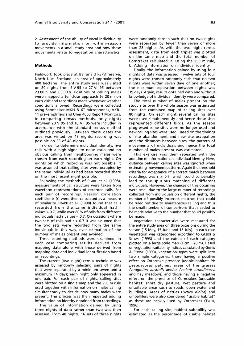
Animal Biodiversity and Conservation 24.1 (2001) 83
2. Assessment of the ability of vocal individualityto provide information on within–seasonmovements in a small study area and how thesemovements relate to vegetation characteristics.
Methods
Fieldwork took place at Balranald RSPB reserve,North Uist, Scotland, an area of approximately400 hectares. The entire study area was visitedon 80 nights from 5 V 95 to 27 VII 95 between23.00 h and 03.00 h. Positions of calling maleswere mapped after close approach (< 20 m) oneach visit and recordings made whenever weatherconditions allowed. Recordings were collectedusing Sennheiser MKH–816T microphones, AKB–11 pre–amplifiers and Uher 4000 Report Monitors.In comparing census methods, only nightsbetween 20 V 95 and 10 VII 95 were included inaccordance with the standard census methodoutlined previously. Between these dates thearea was visited on 48 nights; recording waspossible on 33 of 48 nights.
In order to determine individual identity, fivecalls with a high signal–to–noise ratio and noobvious calling from neighbouring males werechosen from each recording on each night. Onnights on which recording was not possible, itwas assumed that calling sites were occupied bythe same individual as had been recorded thereon the most recent night possible.
Following the methods of PEAKE et al. (1998),measurements of call structure were taken fromwaveform representations of recorded calls. Foreach pair of recordings, Pearson correlationcoefficients (r) were then calculated as a measureof similarity. PEAKE et al. (1998) found that callsrecorded from the same individual had rvalues > 0.7, while over 80% of calls from differentindividuals had r values < 0.7. On occasions wheretwo sets of calls had r > 0.7 it was assumed thatthe two sets were recorded from the sameindividual; in this way, over–estimation of thenumber of males present was avoided.
Three counting methods were examined, ineach case comparing results derived frommapping data alone with those derived frommapping data and individual identification basedon recordings.
The current (two–night) census technique wasassessed by randomly selecting pairs of nightsthat were separated by a minimum seven and amaximum 14 days; each night only appeared inone pair. For each pair of nights, calling siteswere plotted on a single map and the 250 m ruleused together with information on males callingsimultaneously to decide how many males werepresent. This process was then repeated addinginformation on identity obtained from recordings.
The value of information gained by usingthree nights of data rather than two was thenassessed. From 48 nights, 16 sets of three nights
were randomly chosen such that no two nightswere separated by fewer than seven or morethan 28 nights. As with the two night censusassessment, data from each triplet was plottedon the same map and the total number ofCorncrakes calculated: a. Using the 250 m rule,b. Adding information on individual identity.
Finally, the information gained by using fournights of data was assessed. Twelve sets of fournights were chosen randomly such that no twonights were within seven days of one another;the maximum separation between nights was39 days. Again, results obtained with and withoutknowledge of individual identity were compared.
The total number of males present on thestudy site over the whole season was estimatedfrom the combined map of calling sites over80 nights. On each night several calling siteswere used simultaneously and hence those sitesrepresented different birds. As the seasonprogressed some sites were no longer used andnew calling sites were used. Based on the timingsof site abandonment and new site occupationand the distances between sites, the pattern ofmovements of individuals and hence the totalnumber of males present was estimated.
This exercise was then repeated with theaddition of information on individual identity. Here,distance between calling sites was ignored whenestimating movement patterns. Again the thresholdcriteria for acceptance of a correct match betweenrecordings was r > 0.7, which could conceivablylead to the spurious matching of differentindividuals. However, the chances of this occurringwere small due to the large number of recordingscollected from individuals on different nights, thenumber of possibly incorrect matches that couldbe ruled out due to simultaneous calling and thusthe small number of comparisons that needed tobe made relative to the number that could possiblybe made.
Vegetation characteristics were measured forthe entire study area on three occasions during theseason (15 May, 15 June and 15 July). In each casevegetation was categorised according to GREEN &STOWE (1993) and the extent of each categoryplotted on a large scale map (1 cm = 20 m). Basedon vegetation suitability indices calculated by GREEN
& STOWE (1993), vegetation types were split intotwo simple categories: those having a positiveeffect on Corncrake presence (usable habitat: Irispseudacorus patches, areas of the grassesPhragmites australis and/or Phalaris arundinaceaand hay meadows) and those having a negativeeffect on the presence of Corncrakes (unusablehabitat: short dry pasture, wet pasture andunsuitable areas such as roads, open water andbuildings). Areas of nettles (Urtica dioica) andumbellifers were also considered "usable habitat"as these are heavily used by Corncrakes (TYLER,1996).
For each calling site, habitat suitability wasestimated as the percentage of usable habitat
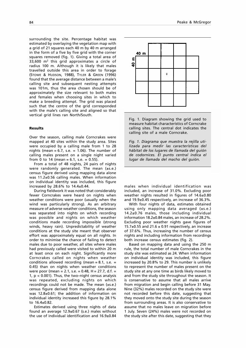
84 Peake & McGregor
surrounding the site. Percentage habitat wasestimated by overlaying the vegetation map witha grid of 21 squares each 40 m by 40 m arrangedin the form of a five by five grid with the cornersquares removed (fig. 1). Giving a total area of33,600 m2 this grid approximates a circle ofradius 100 m. Although it is likely that malestravelled outside this area in order to forage(STOWE & HUDSON, 1988), TYLER & GREEN (1996)found that the average distance between a male’scalling site and subsequent nesting attemptswas 101m, thus the area chosen should be ofapproximately the size relevant to both malesand females when choosing sites in which tomake a breeding attempt. The grid was placedsuch that the centre of the grid correspondedwith the male’s calling site and aligned so thatvertical grid lines ran North/South.
Results
Over the season, calling male Corncrakes weremapped at 40 sites within the study area. Siteswere occupied by a calling male from 1 to 28nights (mean = 6.7, s.e. = 1.06). The number ofcalling males present on a single night variedfrom 0 to 14 (mean = 6.1, s.e. = 0.55).
From a total of 48 nights, 24 pairs of nightswere randomly generated. The mean (±s.e.)census figure derived using mapping data alonewas 11.2±0.56 calling males. When informationon individual identity was included, this figureincreased by 28.6% to 14.4±0.44.
During fieldwork it was noted that considerablyfewer Corncrakes were heard on nights whenweather conditions were poor (usually when thewind was particularly strong). As an arbitrarymeasure of adverse weather conditions, the seasonwas separated into nights on which recordingwas possible and nights on which weatherconditions made recording impossible (strongwinds, heavy rain). Unpredictability of weatherconditions at the study site meant that observereffort was approximately equal on all nights. Inorder to minimise the chance of failing to detectmales due to poor weather, all sites where maleshad previously called were visited to within 20 mat least once on each night. Significantly moreCorncrakes called on nights when weatherconditions allowed recording (mean = 8.1, s.e. =0.45) than on nights when weather conditionswere poor (mean = 2.1, s.e. = 0.48, H = 27.7, d.f. =1, p < 0.001). Thus, the two–night census analysiswas repeated, excluding nights on whichrecordings could not be made. The mean (±s.e.)census figure derived from mapping data alonewas 12.8±0.61; the addition of information onindividual identity increased this figure by 28.1%to 16.4±0.82.
Estimates derived using three nights of datafound an average 12.9±0.67 (s.e.) males withoutthe use of individual identification and 16.9±0.84
males when individual identification wasincluded, an increase of 31.0%. Excluding poorweather nights resulted in figures of 14.6±0.80and 19.9±0.45 respectively, an increase of 36.3%.
With four nights of data, estimates obtainedusing only mapping data averaged (±s.e.)14.2±0.76 males, those including individualinformation 18.2±0.84 males, an increase of 28.2%.Excluding poor weather nights gave figures of15.7±0.55 and 21.6 ± 0.91 respectively, an increaseof 37.6%. Thus, increasing the number of censusnights and including information from recordingsboth increase census estimates (fig. 2).
Based on mapping data and using the 250 mrule, the total number of male Corncrakes in thestudy site was estimated as 24. When informationon individual identity was included, this figureincreased by 20.8% to 29. This number is unlikelyto represent the number of males present on thestudy site at any one time as birds likely moved toand from the study site throughout the season. Itis conservative to assume that all males arrivefrom migration and begin calling before 31 May.Nine (32%) males recorded on the study site werenot recorded before this date, suggesting thatthey moved onto the study site during the seasonfrom surrounding areas. It is also conservative toassume that no males leave on migration before1 July. Seven (24%) males were not recorded onthe study site after this date, suggesting that they
Fig. 1. Diagram showing the grid used tomeasure habitat characteristics of Corncrakecalling sites. The central dot indicates thecalling site of a male Corncrake.
Fig. 1. Diagrama que muestra la rejilla uti-lizada para medir las características delhábitat de los lugares de llamada del guiónde codornices. El punto central indica ellugar de llamada del macho del guión.
40 m40 m40 m40 m40 m
40
m4
0 m
40
m4
0 m
40
m
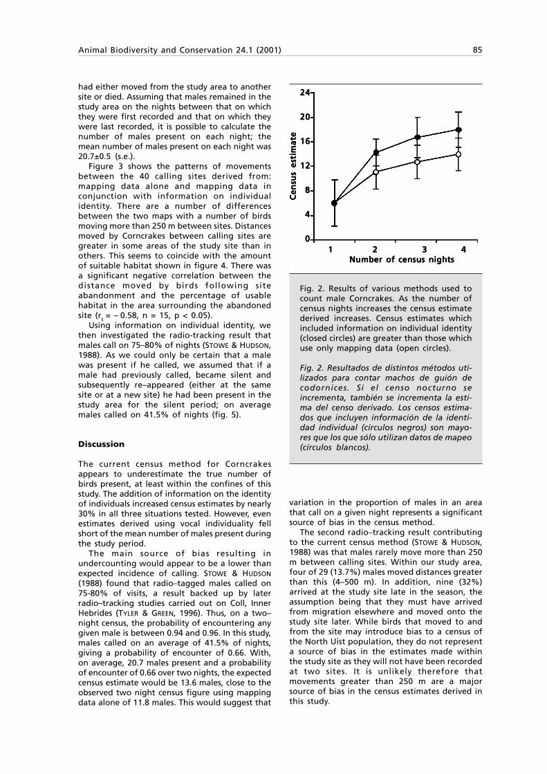
Animal Biodiversity and Conservation 24.1 (2001) 85
had either moved from the study area to anothersite or died. Assuming that males remained in thestudy area on the nights between that on whichthey were first recorded and that on which theywere last recorded, it is possible to calculate thenumber of males present on each night; themean number of males present on each night was20.7±0.5 (s.e.).
Figure 3 shows the patterns of movementsbetween the 40 calling sites derived from:mapping data alone and mapping data inconjunction with information on individualidentity. There are a number of differencesbetween the two maps with a number of birdsmoving more than 250 m between sites. Distancesmoved by Corncrakes between calling sites aregreater in some areas of the study site than inothers. This seems to coincide with the amountof suitable habitat shown in figure 4. There wasa significant negative correlation between thedistance moved by birds following siteabandonment and the percentage of usablehabitat in the area surrounding the abandonedsite (rs = – 0.58, n = 15, p < 0.05).
Using information on individual identity, wethen investigated the radio-tracking result thatmales call on 75–80% of nights (STOWE & HUDSON,1988). As we could only be certain that a malewas present if he called, we assumed that if amale had previously called, became silent andsubsequently re–appeared (either at the samesite or at a new site) he had been present in thestudy area for the silent period; on averagemales called on 41.5% of nights (fig. 5).
Discussion
The current census method for Corncrakesappears to underestimate the true number ofbirds present, at least within the confines of thisstudy. The addition of information on the identityof individuals increased census estimates by nearly30% in all three situations tested. However, evenestimates derived using vocal individuality fellshort of the mean number of males present duringthe study period.
The main source of bias resulting inundercounting would appear to be a lower thanexpected incidence of calling. STOWE & HUDSON
(1988) found that radio–tagged males called on75-80% of visits, a result backed up by laterradio–tracking studies carried out on Coll, InnerHebrides (TYLER & GREEN, 1996). Thus, on a two–night census, the probability of encountering anygiven male is between 0.94 and 0.96. In this study,males called on an average of 41.5% of nights,giving a probability of encounter of 0.66. With,on average, 20.7 males present and a probabilityof encounter of 0.66 over two nights, the expectedcensus estimate would be 13.6 males, close to theobserved two night census figure using mappingdata alone of 11.8 males. This would suggest that
variation in the proportion of males in an areathat call on a given night represents a significantsource of bias in the census method.
The second radio–tracking result contributingto the current census method (STOWE & HUDSON,1988) was that males rarely move more than 250m between calling sites. Within our study area,four of 29 (13.7%) males moved distances greaterthan this (4–500 m). In addition, nine (32%)arrived at the study site late in the season, theassumption being that they must have arrivedfrom migration elsewhere and moved onto thestudy site later. While birds that moved to andfrom the site may introduce bias to a census ofthe North Uist population, they do not representa source of bias in the estimates made withinthe study site as they will not have been recordedat two sites. It is unlikely therefore thatmovements greater than 250 m are a majorsource of bias in the census estimates derived inthis study.
Fig. 2. Results of various methods used tocount male Corncrakes. As the number ofcensus nights increases the census estimatederived increases. Census estimates whichincluded information on individual identity(closed circles) are greater than those whichuse only mapping data (open circles).
Fig. 2. Resultados de distintos métodos uti-lizados para contar machos de guión decodornices. Si el censo nocturno seincrementa, también se incrementa la esti-ma del censo derivado. Los censos estima-dos que incluyen información de la identi-dad individual (círculos negros) son mayo-res que los que sólo utilizan datos de mapeo(círculos blancos).
2424242424
2020202020
1616161616
1212121212
88888
44444
0000011111 22222 33333 44444 Number of census nights Number of census nights Number of census nights Number of census nights Number of census nights
Ce
nsu
s e
stim
ate
Ce
nsu
s e
stim
ate
Ce
nsu
s e
stim
ate
Ce
nsu
s e
stim
ate
Ce
nsu
s e
stim
ate
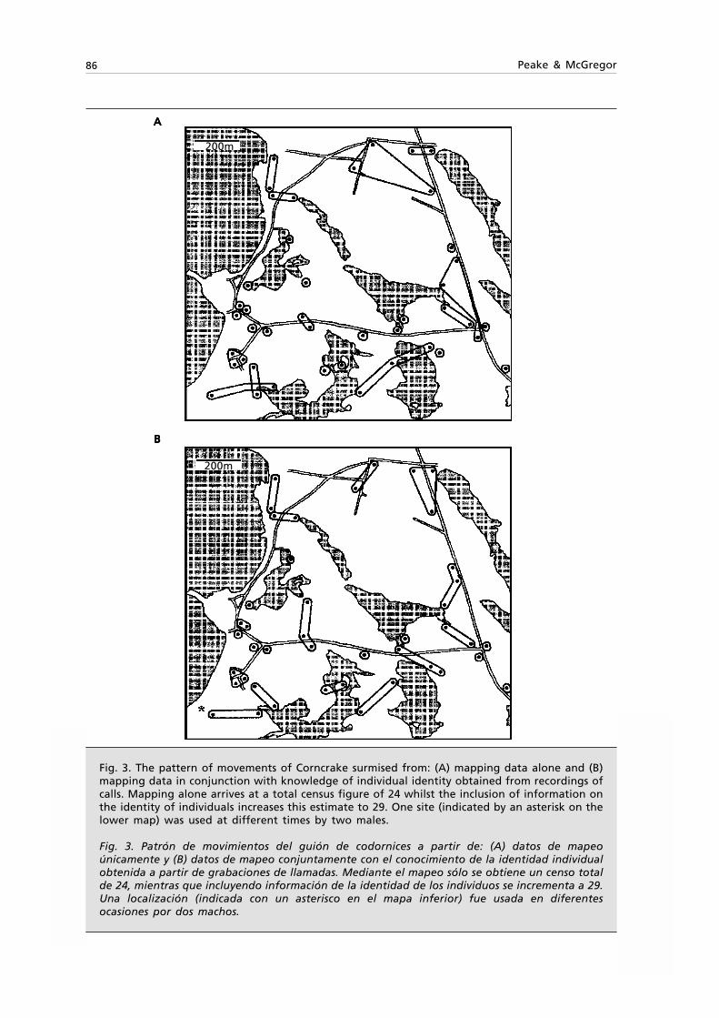
86 Peake & McGregor
Fig. 3. The pattern of movements of Corncrake surmised from: (A) mapping data alone and (B)mapping data in conjunction with knowledge of individual identity obtained from recordings ofcalls. Mapping alone arrives at a total census figure of 24 whilst the inclusion of information onthe identity of individuals increases this estimate to 29. One site (indicated by an asterisk on thelower map) was used at different times by two males.
Fig. 3. Patrón de movimientos del guión de codornices a partir de: (A) datos de mapeoúnicamente y (B) datos de mapeo conjuntamente con el conocimiento de la identidad individualobtenida a partir de grabaciones de llamadas. Mediante el mapeo sólo se obtiene un censo totalde 24, mientras que incluyendo información de la identidad de los individuos se incrementa a 29.Una localización (indicada con un asterisco en el mapa inferior) fue usada en diferentesocasiones por dos machos.
200m
200m
AAAAA
BBBBB

Animal Biodiversity and Conservation 24.1 (2001) 87
However, the effects of the movement ofindividuals on census estimates may be greater insome areas than others. It appears from this studythat where suitable habitat is scarce or patchilydistributed, male Corncrakes move greaterdistances throughout the season than in areaswhere habitat is more homogenous. Where areasdiffer greatly in habitat availability or continuity,census figures may be difficult to compare directly.Perhaps more importantly, where habitat withina given site changes over time, whether for better(positive habitat management) or for worse(habitat destruction), movement rates, and hencecensus inaccuracy, are likely to change. This couldresult in trends become obscured or accentuateddepending on the direction of habitat change.Having an idea of the levels of inaccuracy withinand between given areas and/or years wouldenable this problem to be counteracted to someextent.
There are several reasons why the results ofthis study might differ from those achieved byradio-tracking. Radio–tracking studies carried outby STOWE & HUDSON (1988, 1991) took place in twoareas, three km and 50 km south of our study site.It is possible that geographical variation in habitatbetween these areas and our study area mayhave resulted in behavioural differences between
the males in each study. This is perhaps less likelythan the fact that these previous studies werecarried out between eight and ten years beforethis study; during that time, changes in agriculturalpractices may have had a greater effect on habitatthan subtle geographic differences.
It is also possible that radio–tracking itselfaffected the behaviour of male Corncrakesstudied previously. There are two main sourcesof potential bias involved in radio–trackingstudies. Firstly, the method of capturing maleCorncrakes may not capture a random sample ofthe population. Males are usually captured usingplayback of calls to stimulate approach. It ispossible that this procedure biases capture ratestowards a certain behavioural subset of maleCorncrakes, e.g. those that are more stronglyterritorial and thus more vocally active. Second,radio-tags themselves may have caused changesin the behaviour of males. Male Corncrakesappear only to call nocturnally while attemptingto attract a mate, becoming silent at night oncesuccessful (TYLER & GREEN, 1996). Radio–tags mayreduce mating opportunities, resulting in anincrease in the amount of time spent calling.However, TYLER (1996) found no difference in theattraction of radio–tagged females to taggedand untagged males.
Fig. 4. Map showing the percentage cover of habitat suitable for Corncrake in 100x100 m2 squaresthroughout the study area. Closed circles represent calling sites of male corncrake; lines connectingsites indicate movements between sites.
Fig. 4. Mapa que muestra el porcentaje de cobertura de hábitat disponible para el guión de codornicesen cuadrículas de 100x100 m2 del área de estudio. Los círculos negros representan los sitios de llamadade machos de guión; las líneas que los conectan indican movimientos entre estos sitios.
< 5%< 5%< 5%< 5%< 5%5–14%5–14%5–14%5–14%5–14%15–24%15–24%15–24%15–24%15–24%>25%>25%>25%>25%>25%
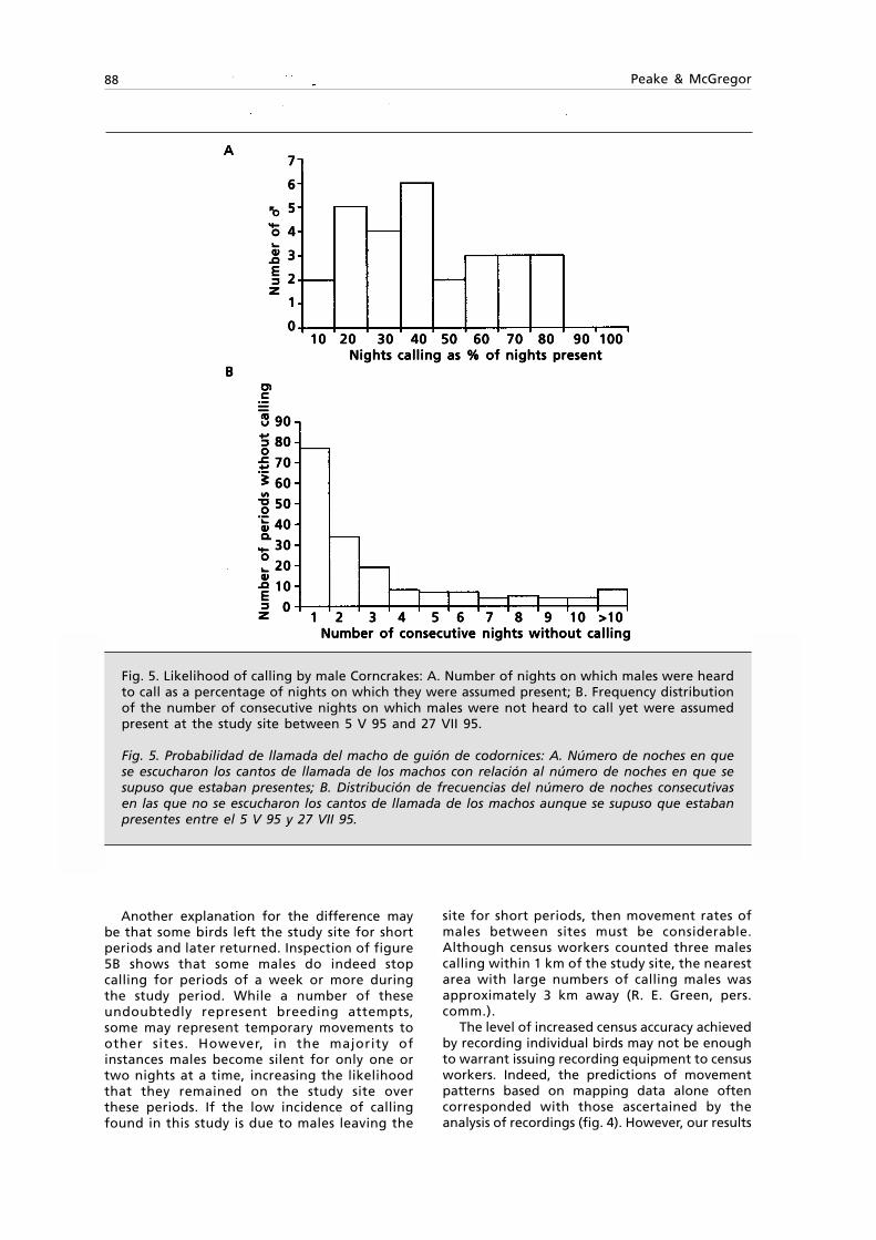
88 Peake & McGregor
Another explanation for the difference maybe that some birds left the study site for shortperiods and later returned. Inspection of figure5B shows that some males do indeed stopcalling for periods of a week or more duringthe study period. While a number of theseundoubtedly represent breeding attempts,some may represent temporary movements toother sites. However, in the majority ofinstances males become silent for only one ortwo nights at a time, increasing the likelihoodthat they remained on the study site overthese periods. If the low incidence of callingfound in this study is due to males leaving the
site for short periods, then movement rates ofmales between sites must be considerable.Although census workers counted three malescalling within 1 km of the study site, the nearestarea with large numbers of calling males wasapproximately 3 km away (R. E. Green, pers.comm.).
The level of increased census accuracy achievedby recording individual birds may not be enoughto warrant issuing recording equipment to censusworkers. Indeed, the predictions of movementpatterns based on mapping data alone oftencorresponded with those ascertained by theanalysis of recordings (fig. 4). However, our results
Fig. 5. Likelihood of calling by male Corncrakes: A. Number of nights on which males were heardto call as a percentage of nights on which they were assumed present; B. Frequency distributionof the number of consecutive nights on which males were not heard to call yet were assumedpresent at the study site between 5 V 95 and 27 VII 95.
Fig. 5. Probabilidad de llamada del macho de guión de codornices: A. Número de noches en quese escucharon los cantos de llamada de los machos con relación al número de noches en que sesupuso que estaban presentes; B. Distribución de frecuencias del número de noches consecutivasen las que no se escucharon los cantos de llamada de los machos aunque se supuso que estabanpresentes entre el 5 V 95 y 27 VII 95.
1010101010 2020202020 3030303030 4040404040 5050505050 6060606060 7070707070 8080808080 9090909090 100100100100100 Nights calling as % of nights present Nights calling as % of nights present Nights calling as % of nights present Nights calling as % of nights present Nights calling as % of nights present
11111 22222 33333 44444 55555 66666 77777 88888 99999 1010101010 >10>10>10>10>10 Number of consecutive nights without calling Number of consecutive nights without calling Number of consecutive nights without calling Number of consecutive nights without calling Number of consecutive nights without calling
77777
66666
55555
44444
33333
22222
11111
00000
Nu
mb
er
of
{N
um
be
r o
f {
Nu
mb
er
of
{N
um
be
r o
f {
Nu
mb
er
of
{
9090909090
8080808080
7070707070
6060606060
5050505050
4040404040
3030303030
2020202020
1010101010
00000
Nu
mb
er
of
pe
rio
ds
wit
ho
ut
call
ing
Nu
mb
er
of
pe
rio
ds
wit
ho
ut
call
ing
Nu
mb
er
of
pe
rio
ds
wit
ho
ut
call
ing
Nu
mb
er
of
pe
rio
ds
wit
ho
ut
call
ing
Nu
mb
er
of
pe
rio
ds
wit
ho
ut
call
ing
AAAAA
BBBBB

Animal Biodiversity and Conservation 24.1 (2001) 89
suggest that the sources and extents of bias incensus estimates may differ between areas,potentially making comparison difficult. Therelative accuracy of a census in a given area at agiven time can be assessed relatively quickly andeasily using the vocal individuality techniquewithout the need to capture or otherwise disturbindividual males.
Individually distinct vocalisations can have avery direct application in the detection ofbreeding attempts. Results of recent studies ofradio-tagged individuals suggest that males ceasenocturnal calling when accompanied by a female(TYLER & GREEN, 1996) and thus that cessation ofnocturnal calling gives an indication of attemptedbreeding. However, this method relies on theassumption that subsequent calling at a givensite is produced by the previously resident maleand cannot detect males that move largedistances following breeding attempts. It is onlypossible to confirm the identity of a residentmale if that male is either ringed (requiringcapture on at least two occasions), radio–tagged(expensive and requires capture) or throughanalysis of recorded calls (requires sophisticatedequipment but not capture).
Despite a growing number of studies thatexamine the potential of vocal individuality toprovide ecological information, there is littlepublished evidence that such techniques are usedor indeed are useful in practice. This study hasdemonstrated that individual distinctivenesspresent in the calls of the Corncrake (MAY, 1994;PEAKE et al., 1998) can provide information thatis of comparable accuracy to informationcollected by other techniques. More importantly,individually distinct calls provide an opportunityto assess relative accuracy.
Acknowledgements
TMP was supported by a CASE studentshipbetween the BBSRC and the RSPB. Analysisequipment was funded by NERC and the RoyalSociety. We are grateful to Rhys Green, KenSmith, Ken Otter and Andrew Terry for commentsthat improved the manuscript considerably. Weare also grateful to Phil Benstead, Cath Jeffs,Alex Turner and Dave Hodson for help andhospitality during fieldwork in North Uist.Fieldwork was carried out under licence SCB:02:95from Scottish Natural Heritage.
References
BIBBY, C. J., BURGESS, N. D. & HILL, D. A., 1992. BirdCensus Techniques. Academic Press, London.
COLLAR, N. J. & ANDREW, P., 1988. Birds to watch:The ICBP World checklist of threatened birds.ICBP, London.
DAHLQUIST, F. C., SCHEMNITZ, S. D. & FLACHS, B. K.,
1990. Distinguishing individual male wildturkeys by analyzing vocalisations using apersonal computer. Bioacoustics, 2: 303–316.
DUFAULT, S. & WHITEHEAD, H., 1995. An assessmentof changes with time in the marking patternsused for photo–identification of individualsperm whales, Physeter macrocephalus. MarineMammal Science, 11: 335–243.
GALEOTTI, P., 1994. Patterns of territory size anddefence level in rural and urban tawny owl(Strix aluco) populations. J. Zool. (Lond.), 234:641–658
GALEOTTI, P. & PAVAN, G., 1991. Individualrecognition of male tawny owls (Strix aluco)using spectrograms of their territorial calls.Ethol. Ecol. Evol., 3: 113–126.
GIBBS, J. P. & WENNY, D.G., 1993. Song output as apopulation estimator: effect of male pairingstatus. J. Field. Ornith., 64: 316–322.
GILBERT, G., GIBBONS, D. W. & EVANS, J., 1998. BirdMonitoring Manual: a compendium ofmonitoring and survey techniques for birdsof conservation concern and others in theUK. RSPB/BTO/WWT/JNCC/ITE/Seabird Group,Sandy, UK.
GILBERT, G., MCGREGOR, P. K. & TYLER, G., 1994.Vocal individuality as a census tool, practicalconsiderations illustrated by a study of tworare species. J. Field Ornith., 65: 335–348.
GREEN, R. E., 1995. The decline of the CorncrakeCrex crex in Britain continues. Bird Study, 42:66–75.
GREEN, R. E. & STOWE, T. J., 1993. The decline ofthe corncrake Crex crex in Britain and Irelandin relation to habitat change. J. Appl. Ecol.,30: 689–695.
HUDSON, A.V., STOWE, T. J. & ASPINALL, S. J., 1990.Status and distribution of corncrakes in Britainin 1988. British Birds, 83: 173–187.
KREBS, C. J., 1989. Ecological Methodology. Harperand Row, New York.
MAY, L., 1994. Individually distinctive CorncrakeCrex crex calls: A pilot study. Bioacoustics, 6:25–32.
MCGREGOR, P. K. & PEAKE, T. M., 1998. The roleof individual identification in conservationbiology. In: Behavioural Ecology andConservation Biology: 31–55 (T. M. Caro, Ed.).Oxford University Press, Oxford.
PEAKE, T. M., MCGREGOR, P. K., SMITH, K. W., TYLER,G., GILBERT, G. & GREEN, R. E., 1998. Individualityin Corncrake Crex crex vocalisations. Ibis, 140:120–127.
POLLARD, E. & YATES, T. J., 1993. Monitoringbutterflies for ecology and conservation.Chapman Hall, London.
SAUNDERS, P. A. & WOOLLER, R. D., 1988. Consistentindividuality of voice in birds as a managementtool. Emu, 88: 25–32.
SOUTHWOOD, T. R. E., 1978. Ecological Methods.Chapman Hall, London.
STONEHOUSE, B., 1978. Animal marking of animalsin research. Macmillan, London.

90 Peake & McGregor
STOWE, T. J. & HUDSON, A. V., 1988. Corncrakestudies in the western isles. RSPB Cons. Rev., 2:38–42.
– 1991. Radio–telemetry studies of corncrakesin Great Britain. Vogelwelt, 112: 10–16.
SUTHERLAND, W. J., 1996. Ecological censustechniques. Cambridge University Press,Cambridge.
TYLER, G., 1996. The ecology of the corncrakewith special reference to the effect of mowingon breeding production. Ph. D. Thesis,University College Cork.
TYLER, G. & GREEN, R. E., 1996. The incidence ofnocturnal song by male Corncrakes Crex crexis reduced during pairing. Bird Study, 43:214–219.

91Animal Biodiversity and Conservation 24.1 (2001)
© 2001 Museu de ZoologiaISSN: 1578–665X
Ricketts, T. H., 2001. Aligning conservation goals: are patterns of species richness and endemism concordantat regional scales? Animal Biodiversity and Conservation, 24.1: 91–99.
AbstractAbstractAbstractAbstractAbstractAligning conservation goals: are patterns of species richness and endemism concordant at regional scales?—Biodiversity conservation strategies commonly target areas of high species richness and/or high endemism.However, the correlation between richness and endemism at scales relevant to conservation is unclear; thesetwo common goals of conservation plans may therefore be in conflict. Here the spatial concordance betweenrichness and endemism is tested using five taxa in North America: butterflies, birds, mammals, amphibians, andreptiles. This concordance is also tested using overall indices of richness and endemism (incorporating all fivetaxa). For all taxa except birds, richness and endemism were significantly correlated, with amphibians, reptiles,and the overall indices showing the highest correlations (rs = 0.527–0.676). However, “priority sets” ofecoregions (i.e., the top 10% of ecoregions) based on richness generally overlapped poorly with those basedon endemism (< 50% overlap for all but reptiles). These results offer only limited support for the idea thatrichness and endemism are correlated at broad scales and indicate that land managers will need to balancethese dual, and often conflicting, goals of biodiversity conservation.
Key words: Conservation goals, Species richness, Endemism, Regional scales.
ResumenResumenResumenResumenResumenAjuste de los objetivos de conservación ¿Son concordantes a escala regional los patrones de riqueza de especiesy de endemismos?— Las estrategias de conservación de la biodiversidad se centran habitualmente en áreas conuna gran riqueza de especies y/o un alto nivel de endemicidad. Sin embargo, la correlación entre riqueza yendemismo a escala relevante para la conservación es poco clara; por consiguiente, estos dos objetivoscomunes de los planes de conservación pueden entrar en conflicto. En este trabajo se estudia la concordanciaespacial entre riqueza y endemismo en Norteamérica utilizando cinco taxones: mariposas, aves, mamíferos,anfibios y reptiles. Esta concordancia se estudia también empleando índices globales de riqueza y endemismo(incorporando los cinco taxones). Para todos los taxones, excepto para las aves, riqueza y endemismo aparecencorrelacionados significativamente, mostrando para los anfibios y reptiles una alta correlación de todos losíndices (rs = 0.527–0.676). Sin embargo, las “actuaciones prioritarias” de las ecoregiones (por ejemplo, el 10%de ecoregiones de vanguardia) basadas en la riqueza de especies normalmente se solapan poco con las basadasen endemismos (< 50% de solapamiento para todos los taxones excepto para los reptiles). Estos resultadosapoyan limitadamente la idea de que riqueza y endemismo están correlacionados a gran escala e indica que losgestores del territorio deberán tener en cuenta estos objetivos duales, y a menudo en conflicto entre sí, deconservación de la biodiversidad.
Palabras clave: Objetivos de conservación, Riqueza de especies, Endemismo, Escala regional.
(Recieved: 4 X 01; Final acceptance: 10 X 01)
Taylor H. Ricketts, Center for Conservation Biology, Dept. of Biological Sciences, Gilbert Hall / 371 Serra Mall,Stanford Univ., Stanford, CA 94305–5020 (USA).
Aligning conservation goals: are patternsof species richness and endemismconcordant at regional scales?
T. H. Ricketts
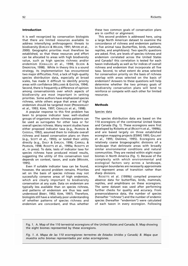
92 Ricketts
Introduction
It is well recognized by conservation biologiststhat there are limited resources available toaddress intensifying anthropogenic threats tobiodiversity (EHRLICH & WILSON, 1991; MYERS et al.,2000). Geographic priorities must therefore beestablished, so that these resources and effortcan be allocated to areas with high biodiversityvalue, such as high species richness and/orendemism (CEBALLOS et al., 1998; OLSON &DINERSTEIN, 1998). While in theory this is a soundstrategy, its implementation has encounteredtwo major difficulties. First, a lack of high–qualityspecies distribution data, especially at broadscales, has made it difficult to identify priorityareas with confidence (WILLIAMS & GASTON, 1994).Second, there is frequently a difference of opinionamong conservationists over which aspects ofbiodiversity are most important in settingpriorities. Some authors have emphasized speciesrichness, while others argue that areas of highendemism should be targeted most (PRENDERGAST
et al., 1993; KERR, 1997; CEBALLOS et al., 1998).A popular response to this first problem has
been to propose indicator taxa: well–studiedgroups of organisms whose richness patterns canbe used as surrogates for other taxa or foroverall species richness. Many recent studies haveeither proposed indicator taxa (e.g., PEARSON &CASSOLA, 1992), assumed them to indicate overallrichness and based conservation plans on them(e.g., SCOTT et al., 1993), or tested their utilitydirectly (e.g., DAILY & EHRLICH, 1996; CARROLL &PEARSON, 1998; RICKETTS et al., 1999a; RICKETTS etal., in press). To date, tests of indicator taxa forspecies richness have produced mixed results,suggesting the utility of this conservation tooldepends on context, taxon, and scale (WEAVER,1995).
Even if suitable indicator taxa can be found,however, the second problem remains. Prioritiesset on the basis of species richness may notsuccessfully conserve areas of high endemism,which are clearly important to biodiversityconservation at any scale. Data on endemism aretypically less available than on species richness,and patterns of endemism are thus less wellunderstood (BIBBY, 1992; KERR, 1997). Therefore,biologists still have a relatively poor understandingof whether patterns of species richness andendemism are concordant, and thus whether
these two common goals of conservation plansare in conflict or alignment.
This second problem is addressed here, usinga large North American dataset to examine theconcordance of richness and endemism patternsin five animal taxa (butterflies, birds, mammals,reptiles, and amphibians). Two specific questionsare asked. First, are levels of species richness andendemism correlated across the United Statesand Canada? this correlation is tested for eachtaxon individually as well as for indices of overallrichness and endemism that incorporate all fivetaxa. Second, to what extent do areas selectedfor conservation priority on the basis of richnessoverlap with areas selected on the basis ofendemism? Answers to these questions will helpdetermine whether the two primary goals ofbiodiversity conservation plans will tend toreinforce or compete with each other for limitedresources.
Methods
Species data
The species distribution data are based on the110 ecoregions of the continental United Statesand Canada (fig. 1). These ecoregions were firstdeveloped by Ricketts et al (RICKETTS et al., 1999b),and are based largely on three establishedecoregion mapping projects (ESWG 1995; GALLANT
et al., 1995; OMERNIK, 1995). Ecoregions arerelatively coarse biogeographic divisions of alandscape that delineate areas with broadlysimilar environmental conditions and naturalcommunities. They are nested within eight majorbiomes in North America (fig. 1). Because of thecomplexity with which environmental andecological factors vary across a landscape,ecoregion boundaries are necessarily approximateand represent areas of transition rather thansharp divisions.
RICKETTS et al. (1999b) compiled presence/absence data for butterflies, birds, mammals,reptiles, and amphibians on these ecoregions.The same dataset was used after performingfurther checks for quality and accuracy. Frompresence/absence data, the number of species(hereafter “richness”) and the number of endemicspecies (hereafter “endemism”) were calculatedof each taxon in every ecoregion. Following
Fig. 1. A. Map of the 110 terrestrial ecoregions of the United States and Canada; B. Map showingthe eight biomes represented by these ecoregions.
Fig. 1. A. Mapa de las 110 ecorregiones terrestres de Estados Unidos y Canadá; B. Mapa quemuestra ocho biomas representados por estas ecorregiones.
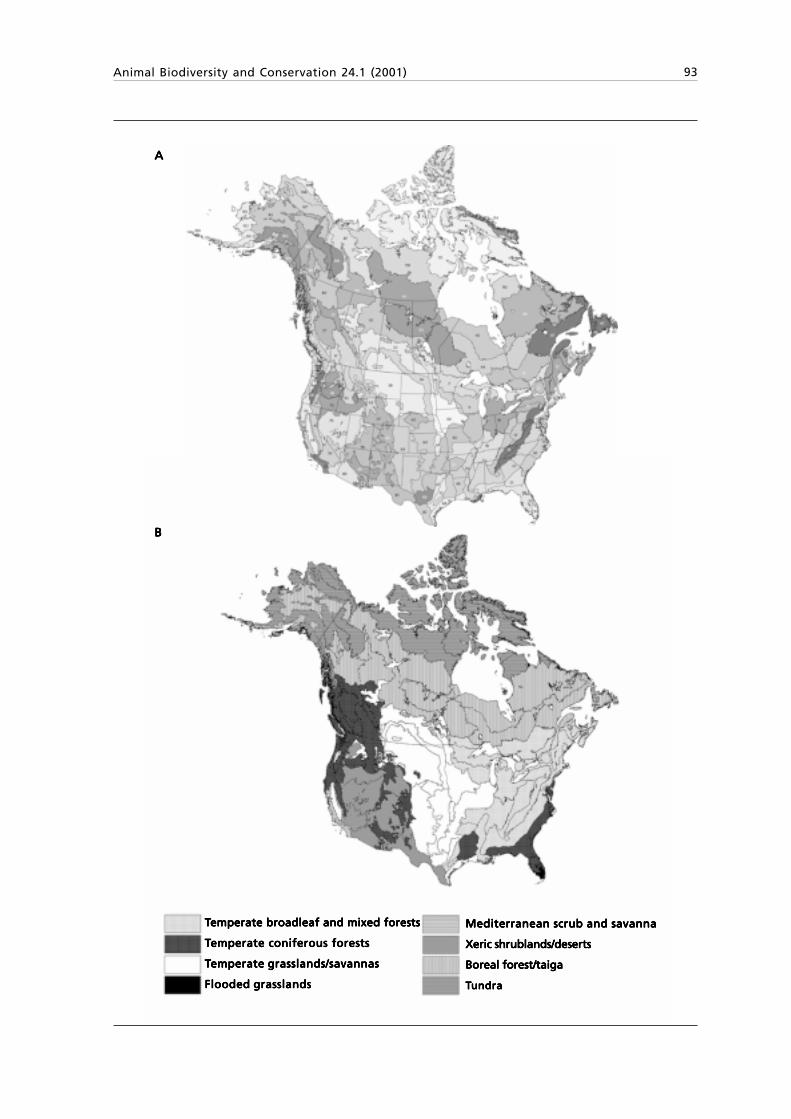
Animal Biodiversity and Conservation 24.1 (2001) 93
TTTTTemperate broadleaf and mixed forestsemperate broadleaf and mixed forestsemperate broadleaf and mixed forestsemperate broadleaf and mixed forestsemperate broadleaf and mixed forests
TTTTTemperate coniferous forestsemperate coniferous forestsemperate coniferous forestsemperate coniferous forestsemperate coniferous forests
TTTTTemperate grasslands/savannasemperate grasslands/savannasemperate grasslands/savannasemperate grasslands/savannasemperate grasslands/savannas
Flooded grasslandsFlooded grasslandsFlooded grasslandsFlooded grasslandsFlooded grasslands
AAAAA
BBBBB
Mediterranean scrub and savannaMediterranean scrub and savannaMediterranean scrub and savannaMediterranean scrub and savannaMediterranean scrub and savanna
Xeric shrublands/desertsXeric shrublands/desertsXeric shrublands/desertsXeric shrublands/desertsXeric shrublands/deserts
Boreal forest/taigaBoreal forest/taigaBoreal forest/taigaBoreal forest/taigaBoreal forest/taiga
TTTTTundraundraundraundraundra
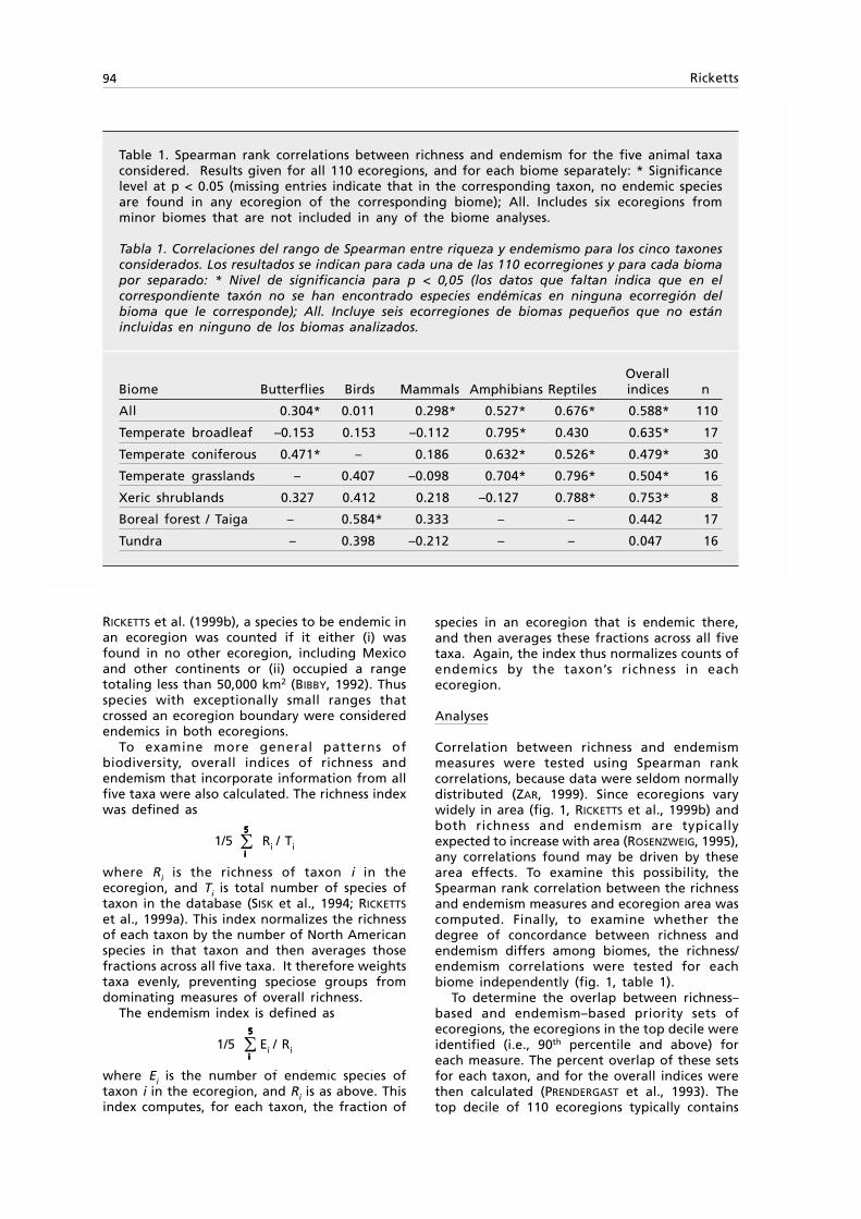
94 Ricketts
RICKETTS et al. (1999b), a species to be endemic inan ecoregion was counted if it either (i) wasfound in no other ecoregion, including Mexicoand other continents or (ii) occupied a rangetotaling less than 50,000 km2 (BIBBY, 1992). Thusspecies with exceptionally small ranges thatcrossed an ecoregion boundary were consideredendemics in both ecoregions.
To examine more general patterns ofbiodiversity, overall indices of richness andendemism that incorporate information from allfive taxa were also calculated. The richness indexwas defined as
1/5 Ri / Ti
where Ri is the richness of taxon i in theecoregion, and Ti is total number of species oftaxon in the database (SISK et al., 1994; RICKETTS
et al., 1999a). This index normalizes the richnessof each taxon by the number of North Americanspecies in that taxon and then averages thosefractions across all five taxa. It therefore weightstaxa evenly, preventing speciose groups fromdominating measures of overall richness.
The endemism index is defined as
1/5 Ei / Ri
where Ei is the number of endemic species oftaxon i in the ecoregion, and Ri is as above. Thisindex computes, for each taxon, the fraction of
species in an ecoregion that is endemic there,and then averages these fractions across all fivetaxa. Again, the index thus normalizes counts ofendemics by the taxon’s richness in eachecoregion.
Analyses
Correlation between richness and endemismmeasures were tested using Spearman rankcorrelations, because data were seldom normallydistributed (ZAR, 1999). Since ecoregions varywidely in area (fig. 1, RICKETTS et al., 1999b) andboth richness and endemism are typicallyexpected to increase with area (ROSENZWEIG, 1995),any correlations found may be driven by thesearea effects. To examine this possibility, theSpearman rank correlation between the richnessand endemism measures and ecoregion area wascomputed. Finally, to examine whether thedegree of concordance between richness andendemism differs among biomes, the richness/endemism correlations were tested for eachbiome independently (fig. 1, table 1).
To determine the overlap between richness–based and endemism–based priority sets ofecoregions, the ecoregions in the top decile wereidentified (i.e., 90th percentile and above) foreach measure. The percent overlap of these setsfor each taxon, and for the overall indices werethen calculated (PRENDERGAST et al., 1993). Thetop decile of 110 ecoregions typically contains
Table 1. Spearman rank correlations between richness and endemism for the five animal taxaconsidered. Results given for all 110 ecoregions, and for each biome separately: * Significancelevel at p < 0.05 (missing entries indicate that in the corresponding taxon, no endemic speciesare found in any ecoregion of the corresponding biome); All. Includes six ecoregions fromminor biomes that are not included in any of the biome analyses.
Tabla 1. Correlaciones del rango de Spearman entre riqueza y endemismo para los cinco taxonesconsiderados. Los resultados se indican para cada una de las 110 ecorregiones y para cada biomapor separado: * Nivel de significancia para p < 0,05 (los datos que faltan indica que en elcorrespondiente taxón no se han encontrado especies endémicas en ninguna ecorregión delbioma que le corresponde); All. Incluye seis ecorregiones de biomas pequeños que no estánincluidas en ninguno de los biomas analizados.
OverallBiome Butterflies Birds Mammals Amphibians Reptiles indices n
All 0.304* 0.011 0.298* 0.527* 0.676* 0.588* 110
Temperate broadleaf –0.153 0.153 –0.112 0.795* 0.430 0.635* 17
Temperate coniferous 0.471* – 0.186 0.632* 0.526* 0.479* 30
Temperate grasslands – 0.407 –0.098 0.704* 0.796* 0.504* 16
Xeric shrublands 0.327 0.412 0.218 –0.127 0.788* 0.753* 8
Boreal forest / Taiga – 0.584* 0.333 – – 0.442 17
Tundra – 0.398 –0.212 – – 0.047 16
✟
✟
55555
iiiii
55555
iiiii
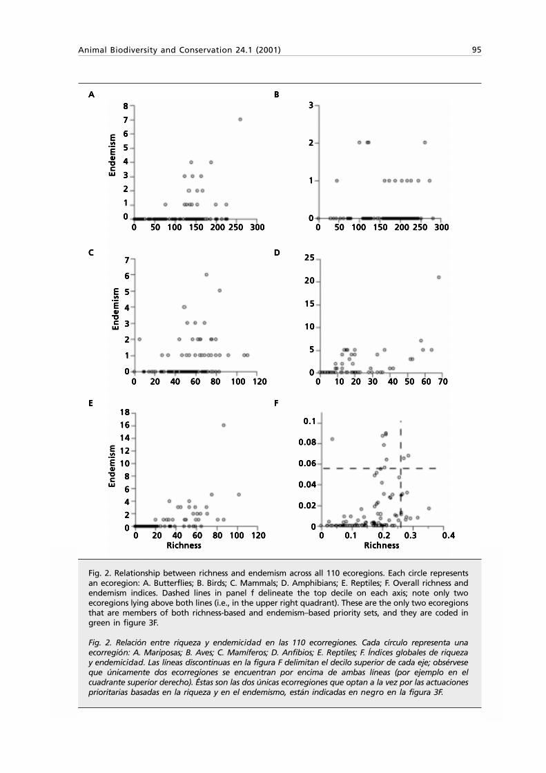
Animal Biodiversity and Conservation 24.1 (2001) 95
AAAAA B B B B B
Fig. 2. Relationship between richness and endemism across all 110 ecoregions. Each circle representsan ecoregion: A. Butterflies; B. Birds; C. Mammals; D. Amphibians; E. Reptiles; F. Overall richness andendemism indices. Dashed lines in panel f delineate the top decile on each axis; note only twoecoregions lying above both lines (i.e., in the upper right quadrant). These are the only two ecoregionsthat are members of both richness-based and endemism–based priority sets, and they are coded ingreen in figure 3F.
Fig. 2. Relación entre riqueza y endemicidad en las 110 ecorregiones. Cada círculo representa unaecorregión: A. Mariposas; B. Aves; C. Mamíferos; D. Anfibios; E. Reptiles; F. Índices globales de riquezay endemicidad. Las líneas discontinuas en la figura F delimitan el decilo superior de cada eje; obsérveseque únicamente dos ecorregiones se encuentran por encima de ambas líneas (por ejemplo en elcuadrante superior derecho). Éstas son las dos únicas ecorregiones que optan a la vez por las actuacionesprioritarias basadas en la riqueza y en el endemismo, están indicadas en negro en la figura 3F.
88888
77777
66666
55555
44444
33333
22222
11111
00000 0 50 100 150 200 250 300 0 50 100 150 200 250 300 0 50 100 150 200 250 300 0 50 100 150 200 250 300 0 50 100 150 200 250 300 0 50 100 150 200 250 300 0 50 100 150 200 250 300 0 50 100 150 200 250 300 0 50 100 150 200 250 300 0 50 100 150 200 250 300
33333
22222
11111
00000
CCCCC D D D D D
EEEEE F F F F F
77777
66666
55555
44444
33333
22222
11111
00000
1818181818
1616161616
1414141414
1212121212
1010101010
88888
66666
44444
22222
00000
0 20 40 60 80 100 120 0 20 40 60 80 100 120 0 20 40 60 80 100 120 0 20 40 60 80 100 120 0 20 40 60 80 100 120 0 10 20 30 40 50 60 70 0 10 20 30 40 50 60 70 0 10 20 30 40 50 60 70 0 10 20 30 40 50 60 70 0 10 20 30 40 50 60 70
2525252525
2020202020
1515151515
1010101010
55555
00000
0.10.10.10.10.1
0.080.080.080.080.08
0.060.060.060.060.06
0.040.040.040.040.04
0.020.020.020.020.02
00000 0 20 40 60 80 100 120 0 20 40 60 80 100 120 0 20 40 60 80 100 120 0 20 40 60 80 100 120 0 20 40 60 80 100 120 0 0.1 0.2 0 0.1 0.2 0 0.1 0.2 0 0.1 0.2 0 0.1 0.2 0.3 0.3 0.3 0.3 0.3 0.40.40.40.40.4
Richness Richness Richness Richness Richness RichnessRichnessRichnessRichnessRichness
En
de
mis
mE
nd
em
ism
En
de
mis
mE
nd
em
ism
En
de
mis
mE
nd
em
ism
En
de
mis
mE
nd
em
ism
En
de
mis
mE
nd
em
ism
En
de
mis
mE
nd
em
ism
En
de
mis
mE
nd
em
ism
En
de
mis
m
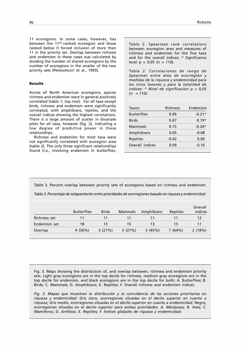
96 Ricketts
11 ecoregions. In some cases, however, tiesbetween the 11th–ranked ecoregion and thoseranked below it forced inclusion of more than11 in the priority set. Overlap between richnessand endemism in these cases was calculated bydividing the number of shared ecoregions by thenumber of ecoregions in the smaller of the twopriority sets (PRENDERGAST et al., 1993).
Results
Across all North American ecoregions, speciesrichness and endemism were in general positivelycorrelated (table 1, top row). For all taxa exceptbirds, richness and endemism were significantlycorrelated, with amphibians, reptiles, and theoverall indices showing the highest correlations.There is a large amount of scatter in bivariateplots for all taxa, however (fig. 2), indicating alow degree of predictive power in theserelationships.
Richness and endemism for most taxa werenot significantly correlated with ecoregion area(table 2). The only three significant relationshipsfound (i.e., involving endemism in butterflies,
Table 2. Spearman rank correlationsbetween ecoregion area and measures ofrichness and endemism for the five taxaand for the overall indices: * Significancelevel p < 0.05 (n = 110).
Tabla 2. Correlaciones de rango deSpearman entre área de ecorregión ymedidas de la riqueza y endemicidad paralos cinco taxones y para la totalidad deíndices: * Nivel de significación p < 0,05(n = 110).
Taxon Richness Endemism
Butterflies 0.09 -0.21*
Birds 0.07 0.19*
Mammals 0.15 -0.26*
Amphibians 0.05 -0.08
Reptiles -0.02 0.00
Overall indices 0.09 -0.16
Table 3. Percent overlap between priority sets of ecoregions based on richness and endemism.
Tabla 3. Porcentaje de solapamiento entre prioridades de ecorregiones basado en riqueza y endemicidad.
Overall Butterflies Birds Mammals Amphibians Reptiles indices
Richness set 11 11 11 11 11 12
Endemism set 18 13 15 13 15 11
Overlap 4 (36%) 3 (27%) 3 (27%) 5 (45%) 7 (64%) 2 (18%)
Fig. 3. Maps showing the distribution of, and overlap between, richness and endemism prioritysets. Light gray ecoregions are in the top decile for richness, medium gray ecoregions are in thetop decile for endemism, and black ecoregions are in the top decile for both: A. Butterflies; B.Birds; C. Mammals; D. Amphibians; E. Reptiles; F. Overall richness and endemism indices.
Fig. 3. Mapas que muestran la distribución y la coincidencia de las acciones prioritarias enriqueza y endemicidad: Gris claro, ecorregiones situadas en el decilo superior en cuanto ariqueza; Gris medio, ecorregiones situadas en el decilo superior en cuanto a endemicidad; Negro,ecorregiones situadas en el decilo superior para ambas prioridades: A. Mariposas; B. Aves; C.Mamíferos; D. Anfibios; E. Reptiles; F. Índices globales de riqueza y endemicidad.

Animal Biodiversity and Conservation 24.1 (2001) 97
AAAAA BBBBB
CCCCC DDDDD
EEEEE FFFFF
98 Ricketts
birds, and mammals) were weak and inconsistentin their sign (table 2). Therefore, the correlationresults in table 1 are unlikely to be caused by thecommonly–expected effects of area on richnessand endemism.
When correlations were tested within eachbiome independently, the results generallyreflected those found using all ecoregions(table 1). Amphibians, reptiles, and the overallindices again tended to show strong correlationsin all but the tundra and taiga biomes.Correlations for butterflies, birds and mammals,which showed weak or no correlation using allecoregions, remained generally non–significantin the biome–by–biome analyses.
Overlap between richness-based and endemism–based priority sets were generally low, varyingbetween 27% (birds and mammals) to 64%(reptiles) (table 3). In addition, priority ecoregionsfor richness and endemism were often found onopposite sides of the continent and often indifferent biomes (fig. 3).
Discussion
These results offer mixed support for the ideathat richness and endemism patterns arecorrelated at broad scales. On one hand, two taxaand the overall indices showed quite strong andconsistent correlations across the 110 ecoregionsand within each major temperate biome (table 1).On the other hand, three of the five taxa showedmuch weaker or no correlations, and the scatterin all of these relationships (and thus theirunpredictability) was high for all taxa.
On the more practical level of choosing areasfor conservation investment, the results are evenless encouraging. Because of the scatter mentionedabove, the statistical correlations found, evenwhen strongly significant, do not translate intohigh overlap between priority sets based onrichness and endemism (table 3, fig. 2). A goodexample is the relationship between the overallrichness and endemism indices (fig. 2F); thestatistical correlation between them is quite high(table 1), but their priority sets overlap in only2 out of a possible 11 ecoregions (table 3). Thiscontradiction is best understood by examiningfigure 2F; although the two variables arecorrelated overall, only two ecoregions fall in thetop decile for both richness and endemism.Indeed, for all taxa except reptiles this overlap isless than 50% (table 3). Basing conservationstrategies on richness, therefore, will seldomeffectively conserve areas of high endemism.
Previous studies on this topic also show amixture of results. In North America, KERR (1997)found relatively strong correlations betweenrichness and endemism in four taxa: mammals, abee genus, a moth subfamily, and a butterflyfamily. PRENDERGAST (1993), however, reported littleconcordance between species–rich hotspots and
rare species in Great Britain, using birds,butterflies, dragonflies, liverworts, and aquaticangiosperms. Similarly, CEBALLOS et al. (1998) found“very low correspondence” among areas of highmammalian richness and endemism in Mexico.
What accounts for the differences in resultsamong these studies? Among other factors,results may be influenced by the taxa and regionconsidered, the scale of observation (both extentand resolution, LEVIN, 1992; PRENDERGAST et al.,1993), the definition of endemism used, and thechoice of geographic units. For example,PRENDERGAST (1993) based their analyses on 10 kmgrid squares in Great Britain, while KERR (1997)used much larger (2.5º of latitude and longitude)grids over a much larger extent in North America(in addition to testing different taxa). Clearlythe four studies (i.e., the three mentioned aboveand mine) differ among themselves in several ofthese factors, making it difficult to glean generallessons from the collective results.
Perhaps of most interest are the contrastingfindings between my study and that of KERR
(1997). These two studies were performed in thesame region at similar scales, with one taxon incommon (mammals). Nevertheless, KERR (1997)found high correlation in mammals (r = 0.807,p < 0.001), while the results presented here showquite a weak relationship (table 1). This differencemay be due to differences in the definition ofendemism. KERR (1997) calculates the endemismvalue of a given square by summing, over allspecies present in the square, the inverses of thenumber of squares occupied by each species(e.g., 1/24+1/137+1/3…). This measure, however,is not independent of richness; the more speciespresent, the more inverses are added to the sum.In contrast, counting the simple number of trueendemics in an area (i.e., species found nowhereelse) is not statistically related to richnessmeasures, and thus may better reveal the actualrelationship between these two measures ofconservation priority.
One caveat deserves mention here. Since atypical species range overlaps with severalecoregions (and thus ecoregions do not accruetheir richnesses independently), these richnessdata probably contain a certain degree of spatialautocorrelation (JONGMAN et al., 1995). Thisproblem tends to inflate the degrees of freedomused in significance testing, and therefore theprobabilities reported here should be interpretedwith caution. However, these results remainuseful for comparing strengths of relationshipsamong taxa, because the correlation coefficientsthemselves are unaffected (only the significancetests). In addition, endemism, by definition, doesnot suffer this same problem.
In conclusion, the results presented here andin other studies (PRENDERGAST et al., 1993; KERR,1997; CEBALLOS et al., 1998) indicate thatconservation biologists may not have the luxuryof assuming that management plans based on

Animal Biodiversity and Conservation 24.1 (2001) 99
“hotspots” of species richness will also captureimportant centers of endemism. Additionalstudies undertaken at different scales and withdifferent taxa may yield a better understandingof the factors that determine the degree ofconcordance between richness and endemismpatterns. Until then, however, conservationbiologists and land managers will need tocontinue to balance these dual, and oftenconflicting, goals of biodiversity conservation.
Acknowledgements
I thank the Conservation Science Program at WorldWildlife Fund–U.S. for their collaboration in originallycompiling these data. K. Bowen, J. Fay, M. Mayfield,and J. Schwan helped to improve, error check, andmanage the databases. C. Boggs, K. Carney, J.Hellmann and J. Hughes provided valuablediscussions and comments on the manuscript. Finally,the support of U.S. NASA and The SummitFoundation are gratefully acknowledged.
References
BIBBY, C. J., 1992. Putting biodiversity on themap: priority areas for global conservation.ICBP, Washington, DC.
CARROLL, S. S. & PEARSON, D. L., 1998. Spatialmodeling of butterfly species richness usingtiger beetles (Cicindelidae) as a bioindicatortaxon. Ecological Applications, 8: 531–543.
CEBALLOS, G., RODRIGUEZ, P. & MEDELLIN, R. A.,1998. Assessing conservation priorities inmegadiverse Mexico: Mammalian diversity,endemicity, and endangerment. EcologicalApplications, 8: 8–17.
DAILY, G. C. & EHRLICH, P. R., 1996. Nocturnalityand species survival. Proceedings of theNational Academy of Sciences of the UnitedStates of America, 93: 11,709–11,712.
EHRLICH, P. R. & WILSON, E. O., 1991. Biodiversitystudies: science and policy. Science, 253: 750–752.
ESWG, 1995. A national ecological framework forCanada. Agriculture and Agri–food Canada,Research Branch, Centre for Land and BiologicalResources Research; and Environment Canada,State of the Environment Directorate, EcozoneAnalysis Branch, Ottawa/Hull.
GALLANT, A. L., BINNIAN, E. F., OMERNIK, J. M. &SHASBY, M. B., 1995. Ecoregions of Alaska. U.S.Geological Survey, Washington, DC.
JONGMAN, R. H. G., TER BRAAK, C. J. F. & VAN
TONGEREN, O. F. R. (Eds.), 1995. Data analysis incommunity and landscape ecology. CambridgeUniversity Press, New York.
KERR, J. T., 1997. Species richness, endemism, andthe choice of areas for conservation.
Conservation Biology, 11: 1,094–1,100.LEVIN, S. A., 1992. The problem of pattern and
scale in ecology. Ecology, 73: 1,943–1,967.MYERS, N., MITTERMEIER, R. A., MITTERMEIER, C. G.,
FONSECA, G. A. B. DA & KENT, J., 2000. Biodiversityhotspots for conservation priorities. Nature,403: 853–858.
OLSON, D. M. & DINERSTEIN, E., 1998. The Global200: A representation approach to conservingthe Earth’s most biologically valuableecoregions. Conservation Biology, 12: 502–515.
OMERNIK, J. M., 1995. Level III ecoregions of thecontinental US. US Environmental ProtectionAgency, Washington, DC.
PEARSON, D. L. & CASSOLA, F., 1992. World–wide speciesrichness patterns of tiger beetles (Coleoptera:Cicindelidae): Indicator taxon for biodiversity andconservation studies. Conservation Biology, 6:376–391.
PRENDERGAST, J. R., QUINN, R. M., LAWTON, J. H.,EVERSHAM, B. C. & GIBBONS, D. W., 1993. Rarespecies, the coincidence of diversity hotspots andconservation strategies. Nature, 365: 335–337.
RICKETTS, T. H., DAILY, G. C. & EHRLICH, P. R. (inpress). Does butterfly diversity predict mothdiversity? Testing a popular indicator taxon atlocal scales. Biological Conservation.
RICKETTS, T. H., DINERSTEIN, E., OLSON, D. M. &LOUCKS, C., 1999a. Who’s where in NorthAmerica: patterns of species richness and theutility of indicator taxa for conservation.Bioscience, 49: 369–381.
RICKETTS, T. H., DINERSTEIN, E., OLSON, D. M., LOUCKS,C., EICHBAUM, W., KAVANAGH, K., HEDAO, P.,HURLEY, P. , CARNEY, K. M., ABEL, R. & WALTERS,S., 1999b. Terrestrial ecoregions of NorthAmerica: A conservation assessment. IslandPress, Washington, DC.
ROSENZWEIG, M. L., 1995. Species diversity in spaceand time. Cambridge University Press,Cambridge.
SCOTT, M. J., DAVIS, F., CSUTI, B., NOSS, R., BUTTERFIELD,B., GROVES, C., ANDERSON, H., CAICCO, S., D’ERCHIA,F., EDWARDS, T. C. J., ULLIMAN, J. & WRIGHT, R. G.,1993. Gap analysis: protecting biodiversityusing geographic information systems. WildlifeMonographs, 123: 1–41.
SISK, T. D., LAUNER, A. E., SWITKY, K. R. & EHRLICH, P.R., 1994. Identifying extinction threats: Globalanalyses of the distribution of biodiversityand the expansion of the human enterprise.BioScience, 44: 592–604.
WEAVER, J. C., 1995. Indicator species and scale ofobservation. Conservation Biology, 9: 939–942.
WILLIAMS, P. H. & GASTON, K. J., 1994. Measuringmore of biodiversity: Can higher–taxon richnesspredict wholesale species richness? BiologicalConservation, 67: 211–217.
ZAR, J. H., 1999. Biostatistical analysis. 4th Edition.Prentice Hall, Upper Saddle River, NJ.

Editor executiu / Editor ejecutivo / Executive Editor Joan Carles Senar
Secretària de Redacció / Secretaria de Redacción / Managing EditorMontserrat Ferrer
Consell Assessor / Consejo asesor / Advisory BoardOleguer EscolàEulàlia GarciaAnna OmedesJosep PiquéFrancesc Uribe
Editors / Editores / Editors Antonio Barbadilla Univ. Autònoma de Barcelona, Bellaterra, SpainXavier Bellés Centre d' Investigació i Desenvolupament CSIC, Barcelona, SpainJuan Carranza Univ. de Extremadura, Cáceres, SpainLuís Mª Carrascal Museo Nacional de Ciencias Naturales CSIC, Madrid, SpainAdolfo Cordero Univ. de Vigo, Vigo, SpainMario Díaz Univ. de Castilla–La Mancha, Toledo, SpainXavier Domingo Univ. Pompeu Fabra, Barcelona, SpainFrancisco Palomares Estación Biológica de Doñana, Sevilla, SpainFrancesc Piferrer Inst. de Ciències del Mar CSIC, Barcelona, SpainIgnacio Ribera The Natural History Museum, London, United KingdomAlfredo Salvador Museo Nacional de Ciencias Naturales, Madrid, SpainJosé Luís Tellería Univ. Complutense de Madrid, Madrid, SpainFrancesc Uribe Museu de Zoologia de Barcelona, Barcelona, Spain
Consell Editor / Consejo editor / Editorial BoardJosé A. Barrientos Univ. Autònoma de Barcelona, Bellaterra, SpainJean C. Beaucournu Univ. de Rennes, Rennes, FranceDavid M. Bird McGill Univ., Québec, CanadaMats Björklund Uppsala Univ., Uppsala, SwedenJean Bouillon Univ. Libre de Bruxelles, Brussels, BelgiumMiguel Delibes Estación Biológica de Doñana CSIC, Sevilla, SpainDario J. Díaz Cosín Univ. Complutense de Madrid, Madrid, SpainAlain Dubois Museum national d’Histoire naturelle CNRS, Paris, FranceJohn Fa Durrell Wildlife Conservation Trust, Trinity, United KingdomMarco Festa–Bianchet Univ. de Sherbrooke, Québec, CanadaRosa Flos Univ. Politècnica de Catalunya, Barcelona, SpainJosep Mª Gili Inst. de Ciències del Mar CMIMA–CSIC, Barcelona, SpainEdmund Gittenberger Rijksmuseum van Natuurlijke Historie, Leiden, The NetherlandsFernando Hiraldo Estación Biológica de Doñana CSIC, Sevilla, SpainPatrick Lavelle Inst. Français de recherche scient. pour le develop. en cooperation, Bondy, FranceSantiago Mas–Coma Univ. de Valencia, Valencia, SpainJoaquín Mateu Estación Experimental de Zonas Áridas CSIC, Almería, SpainNeil Metcalfe Univ. of Glasgow, Glasgow, United KingdomJacint Nadal Univ. de Barcelona, Barcelona, SpainStewart B. Peck Carleton Univ., Ottawa, Canada Eduard Petitpierre Univ. de les Illes Balears, Palma de Mallorca, SpainTaylor H. Ricketts Stanford Univ., Stanford, USAJoandomènec Ros Univ. de Barcelona, Barcelona, SpainValentín Sans–Coma Univ. de Málaga, Málaga, SpainTore Slagsvold Univ. of Oslo, Oslo, Norway
Secretaria de Redacció / Secretaría de Redacción / Editorial Office
Museu de ZoologiaPasseig Picasso s/n08003 Barcelona, SpainTel. +34–93–3196912Fax +34–93–3104999E–mail [email protected]
"La tortue greque" Oeuvres du Comte de Lacépède comprenant L'Histoire Naturelle des Quadrupèdes Ovipares, des Serpents, des Poissons et des Cétacés; Nouvelle édition avec planches coloriées dirigée par M. A. G. Desmarest; Brux-elles: Th. Lejeuné, Éditeur des oeuvres de Buffon, 1836. Pl. 7
Animal Biodiversity and Conservation 24.1, 2001© 2001 Museu de Zoologia, Institut de Cultura, Ajuntament de BarcelonaAutoedició: Montserrat FerrerFotomecànica i impressió: Sociedad Cooperativa Librería GeneralISSN: 1578–665XDipòsit legal: B–16.278–58

101Animal Biodiversity and Conservation 24.1 (2001)
© 2001 Museu de ZoologiaISSN: 1578–665X
Tomás, W. M., McShea, W., Miranda, G. H. B. de, Moreira, J. R., Mourão, G. & Lima Borges, P. A., 2001. Asurvey of a pampas deer, Ozotoceros bezoarticus leucogaster (Arctiodactyla, Cervidae), population in thePantanal wetland, Brazil, using the distance sampling technique. Animal Biodiversity and Conservation, 24.1:101–106.
AbstractAbstractAbstractAbstractAbstractA survey of a pampas deer, Ozotoceros bezoarticus leucogaster (Arctiodactyla, Cervidae), population in the Pantanalwetland, Brazil, using the distance sampling technique.— The pampas deer is an endangered South American specieswhich occurs in open grasslands and savannas. This aim of this survey was to evaluate the use of the distance samplingtechnique to estimate densities of the species in the Pantanal wetland, as well as to analyze the applicability of themethod for a monitoring program. The surveys were conducted on roads from vehicles and also on foot along26 parallel transects in November 1999 and 2000 at Campo Dora ranch, south-central Pantanal, Brazil. Deer densitieswere estimated using the program DISTANCE, and the program MONITOR was used to run a power analysis to estimatethe probability of detection of a decline in the population. The deer density estimated from vehicles, with data fromboth years, was 9.81±3.8 individual/km2, and 5.53±0.68 individuals/km2 from transects sampled on foot. The poweranalysis of these data revealed a monitoring program would require at least two surveys per year over seven years toobtain a 90% chance of detecting a 5% decline in the population. Our results also indicate surveys from roads are notrecommended for pampas deer counts as the animals appear to keep a relatively safe distance from cars.
Key words: Pampas deer, Ozotoceros, Distance sampling technique, Pantanal wetland, Population survey.
ResumenResumenResumenResumenResumenEstudio de una población de venados de la Pampa Ozotoceros bezoartcus leuogaster (Artiodactyla, Cervidae) en elPantanal, Brasil, mediante la técnica del muestreo a distancia.— El venado de la Pampa es una especie sudamericanaen peligro de extinción que se encuentra en praderas abiertas y sabanas. El objetivo de este trabajo es evaluar el usode la técnica de muestreo a distancia para estimar densidades de esta especie en el Pantanal, así como analizar laaplicabilidad de este método a un programa de monitoreo. Los estudios se realizaron desde caminos, con vehículosy a pie, a través de 26 transectos paralelos en noviembre de 1999 y 2000, en la hacienda Campo Dora, Pantanal,Brasil. Las densidades de venados se estimaron con el programa DISTANCE, empleándose el programa MONITORpara efectuar un análisis de poder estimativo para la detección de un descenso en la población de venados. Ladensidad de venados estimada desde los vehículos fue de 9.81±3.8 individuos/km2, mientras la obtenida desdetransectos realizados a pie fue de 5.53±0.68 individuos/km2. Ambas densidades incluyen datos de los dos años deestudio. El análisis potencial de estos datos señala que un programa de monitoreo precisaría como mínimo de dosmuestreos por año, durante siete años, para obtener una probabilidad del 90% de detectar un descenso del 5% enla población. Los resultados de este estudio indican asimismo que las observaciones efectuadas desde caminos noson recomendables para el recuento de venados de la Pampa, ya que se observó que éstos tienden a mantener unadistancia de seguridad respecto a los coches.
Palabras clave: Venados de la Pampa, Ozotoceros, Técnica de muestreo a distancia, Pantanal, Estudio de población.
(Rebut: 20 VII 01; Final acceptance: 1 X 01)
W. M. Tomás, EMBRAPA Recursos Genéticos e Biotecnologia, PqEB, Final W5 Norte, 70770–900 Brasília DF, Brasil.
e–mail: [email protected]
A survey of a pampas deer,Ozotoceros bezoarticus leucogaster(Arctiodactyla, Cervidae), population inthe Pantanal wetland, Brazil, using thedistance sampling technique
W. M. Tomás, W. McShea, G. H. B. de Miranda,J. R. Moreira, G. Mourão & P. A. Lima Borges
102 Tomás et al.
Introduction
The pampas deer (Ozotoceros bezoarticus L.,1758) is a species characteristic of open habitatsin South America, with historic distributionranging from central Argentina to mid–westernand northeastern Brazil, eastern Bolivia, Paraguayand Uruguay (CABRERA, 1943; CARVALHO, 1973;JUNGIUS, 1976; JACKSON & GIULIETTI, 1988; JACKSON
& LANGGUTH, 1987; TOMÁS, 1995). The species isincluded in the International Union forConservation of Nature (IUCN) Red Data Book asa lower risk, near–threatened species (WEMMER,1998); it is also considered endangered by theUnited States Department of Interior–USDI, is inthe Appendix I of Convention International TradeEndangered Species–CITES (CITES, 1995), and islisted as endangered in Brazil (FONSECA et al.,1994). Population declines in this species havebeen attributed to habitat destruction related toagricultural expansion, poaching, and diseasestransmitted by cattle (MERINO et al., 1997).Although surveys and monitoring programs havebeen recommended in conservation action plansfor the species (CBSG, 1993; WEMMER, 1998), littlehas been published on population size estimatesfor this species in Brazil (e.g., LEEUWENBERG &LARA RESENDE, 1994; RODRIGUES, 1996; MOURÃO etal., 2000). The largest population is known tooccur in the Pantanal wetland, and is estimatedat 60,000 individuals (MOURÃO et al., 2000).
MOURÃO et al. (2000) called for long–termmonitoring of pampas deer populations in thePantanal by means of ground surveys, but weknow of no concerted effort to evaluate theappropriate techniques to accomplish this goal.Distance sampling techniques offer potential fora monitoring program because the assumptionsare relatively robust and the protocols can bequickly taught to survey staff (ANDERSON et al.,2001). This survey aims to evaluate the use ofthe distance sampling technique (BURNHAM et al.,1980) to estimate densities of pampas deerthrough transects sampled on foot and/or froma vehicle, as well as to analyze the applicabilityof the method and sampling protocol for amonitoring program of this species.
Material and methods
The survey was conducted in an area of 8,400 ha ofthe Campo Dora ranch (40,000 ha) located 90 kmfrom Corumbá, Mato Grosso do Sul State, Brazil,in the south–central Pantanal wetland. Theaverage annual rainfall is 1,182 mm and theaverage temperature varies from 31.6°C to20.2°C (SORIANO, 1999). The Pantanal vegetationconsists of a mosaic of several forested andopen habitats that vary in topography andflooding regime (PRANCE & SCHALLER, 1982). Theopen habitat is flooded from January to June,with a draining period from July to August.
Lower areas may retain water until October,and some permanent ponds are scatteredthroughout the study area. During the floodingperiod the grassland is substituted by a massiveformation of aquatic macrophytes, which isgradually replaced by grasses as the waterrecedes. The principal economic activity in thestudy area is cattle ranching.
Pampas deer were simultaneously countedfrom vehicles in three different, non–interceptingtransects (roads) on November, 1999, and in thesame month of 2000, between 7.30 and 11.00 a.m.,at a speed of 20 km/h. In each car, one observerstanding in the back of the vehicle recorded thepresence of deer clusters on both sides of theroad. For each sighting, the vehicle stopped andthe perpendicular distance to the road wasmeasured by counting steps, which were thenconverted into meters. The conversion factor hadbeen previously established for each observer.The number of individuals was recorded in eachcluster as observed from the vehicle withoutoptical instruments, as well as the actual numberof deer per cluster, which included any additionalindividual observed afterwards during theperpendicular distance estimation and/or withbinoculars.
Deer were also counted on foot from 12 paralleleast–west oriented transects in November, 1999,and 14 transects in 2000, between 7.30 and 11.00a.m. In 1999, fifteen observers, divided into sixgroups of two or three people, surveyed thetransects starting from a road (with approximatelynorth–south orientation) that traversed the CampoDora ranch. In the 2000 survey, seven groups of atleast 2 observers sampled the south–north andeast–west oriented transects The transects wereseparated by 2 km, with lengths varying from 3 to11 km. Because pampas deer do not use forestedhabitats (MERINO et al., 1997), we excluded theinterception with forest patches from the totallength of each transect. Deer clusters wererecorded using the same protocol defined in thesurvey from vehicles.
Deer cluster densities were estimated usingthe program DISTANCE (LAAKE et al., 1993;BUCKLAND et al., 1993) by selecting the model thatbest fit the data (BURNHAM et al., 1980). The datawere analyzed separately for each year. Thehistograms of observation distributions wereexamined visually and truncated as necessary. Todetermine average cluster sizes and calculatedensities, truncation was based on the definitionof the effectively sampled area given by theprogram DISTANCE to avoid any bias of clustersize being related to the sighting distance.DISTANCE produces a variance estimate that has 3components: the first is the proportion due to theobserver’s ability to detect animals along thetransect; the second due to the variability betweentransect lines; and the third due to variance ingroup size observed.
The program MONITOR (GIBBS, 1995) was used
Animal Biodiversity and Conservation 24.1 (2001) 103
to run a power analysis with the data obtainedfrom the transects surveyed on foot in 1999. Toperform this analysis we need to know the numberof observations expected along each transect andtheir variance. The number of deer/km of transectfor each of the 12 transects surveyed were used inorder to estimate number of observations andcalculate variance. Simulations were made with aone–tailed test, and the amount of effort neededto establish a 90% probability of detecting apopulation decline was estimated as to avoiderror type II. In these simulations we varied: 1.The number of transects per year; 2. The numberof times the sampling would be repeated peryear; 3. The number of years of monitoringnecessary to detect decline.
Results
A total of 58.7 km of transects were surveyed byvehicle in 1999, and 29.5 in 2000. Twenty–sevendeer clusters were detected, with a total of58 individuals in the first year, and 31 clusters(79 individuals) in 2000. The pooled data obtainedby vehicle displayed in figure 1B demonstratethat few deer were observed close to the road,contrasting with the data obtained from thesurveys made on foot (fig. 1A). One criticalassumption with the distance techniques is thatthe further the distance from the survey line, thelower the count (BURNHAM et al., 1980; BUCKLAND
et al., 1993; LAAKE et al., 1993). In order to meetthis assumption we had to truncate observationsup to 100 m from the road, thus reducing theanalysis to 58 clusters. The model which bestfitted our data was a half normal adjustment.The density estimate was 3.63±1.31 clusters/km2
with an average cluster size of 2.38±0.28 deer/cluster. The deer density was estimated to be9.81±3.8 deer/km2. For the vehicular survey, theprobability of detection accounted for 43.9% ofthe variance, the encounter rate 38.7%, and thecluster size 17.4%. The population size wasestimated as 824±318.68 pampas deer.
A total of 77.6 km of transects was surveyed onfoot in 1999. Seventy–eight deer clusters wererecorded in 1999. Unlike the vehicle survey,examination of the data indicated no truncationalong the survey line was necessary. A half normalmodel was found to best fit our data, and effectivesampled width was 163.65±14.75 m. Clusterdensity was estimated as 3.07±0.59 clusters/km2
and the average cluster size as 2.23±0.18individuals. The deer density for our study areawas estimated to be 6.85±1.43 individuals/km2
and the population size was estimated as575±120.16 pampas deer for the Campo Doraranch. The encounter rate (differences betweentransect lines) accounted for 67.3% of observedvariance, leaving 18.6% for detection along thetransect line and 14.1% for cluster size.
A total of 106.51 km of transects was surveyed
on foot in 2000. Ninety–eight deer clusters wererecorded in 2000. A half normal model wasfound to best fit our data, and effective sampledwidth was 175.96±14.02 m. Cluster density wasestimated as 2.61±0.32 clusters/km2 and theaverage cluster size as 1.91±0.13 individuals. Thedeer density for our study area was estimated tobe 4.99±0.70 individuals/km2 and the populationsize was estimated as 419±59.84 pampas deerfor the Campo Dora ranch. The encounter rateaccounted for 45.8% of the variance, with 32.2%of the variance due to detection probability and22.0% to cluster size.
A total of 186 deer clusters was recorded duringthe two sampling periods. The sighting of clusterswas rare 500 m beyond the transects (fig. 1A),with a positive correlation between the log ofcluster size and perpendicular distance from thetransect (r = 0.037, t = 2.65, Df = 184, P = 0.009).The data at this distance was therefore truncated.Analysis of the pooled data from 1999 and 2000indicated that the best model fit was a halfnormal key (fig. 2), and the effective sampledwidth was 181.12±10.76 m. The estimated clusterdensity was 2.68±0.30 clusters/km2, and theaverage cluster size was 2.06±0.10 individuals.The deer density for our study area was estimatedto be 5.53±0.68 individuals/km2 and the populationsize was estimated as 465±57.11 pampas deer.The encounter rate accounted for 59.8% of thevariance, leaving 23.4% for detection probabilityand 16.8% for cluster size.
Our power analysis of the 1999 data revealedthat to obtain a 90% chance of detecting a 5%annual decline in the studied population, atleast two surveys per year for 7 years would benecessary. On the other hand, it would take atleast 10 years with one survey per year to obtaina 90% chance of detecting the same annualdecline. In a shorter time period, three surveysper year would be necessary for 5 years to detecta 7% decline (table 1).
Discussion
Reviewed survey information revealed few studiesof pampas deer whose survey protocols offeredviable data for comparison. RODRIGUES (1996) found1.97±1.38 deer/group and 0.1 deer/km2 for EmasNational Park, applying the distance samplingtechnique to analyze counts obtained from avehicle using roads as transects. LEEUWENBERG &LARA RESENDE (1994) found 1.26 (SD = 0.65) deer/km2
in night counts using strip transects 100 m wide,in the environmental protection area of Gama–Cabeça de Veado, near Brasilia. In northernArgentina, MERINO & BECCACECI (1999) countedpampas deer from an airplane defining a strip of300 m in each side, and found an average groupsize of 1.75±0.78 deer/group, and a density of0.39±0.35 deer/km2. The authors also surveyeddeer from roads using a strip of 300 m on each
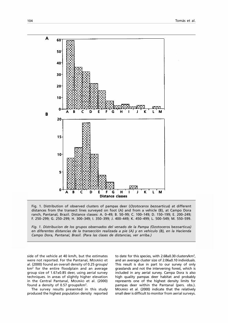
104 Tomás et al.
Fig. 1. Distribution of observed clusters of pampas deer (Ozotoceros bezoarticus) at differentdistances from the transect lines surveyed on foot (A) and from a vehicle (B), at Campo Doraranch, Pantanal, Brazil. Distance classes: A. 0–49; B. 50–99; C. 100–149; D. 150–199; E. 200–249;F. 250–299; G. 250–299; H. 300–349; I. 350–399; J. 400–449; K. 450–499; L. 500–549; M. 550–599.
Fig. 1. Distribucion de los grupos observados del venado de la Pampa (Ozotoceros bezoarticus)en diferentes distancias de la transección realizada a pie (A) y en vehiculo (B), en la HaciendaCampo Dora, Pantanal, Brasil. (Para las clases de distancias, ver arriba.)
6060606060
5050505050
4040404040
3030303030
2020202020
1010101010
00000
2020202020
1515151515
1010101010
55555
00000 A B C D E F G H I J K A B C D E F G H I J K A B C D E F G H I J K A B C D E F G H I J K A B C D E F G H I J K L M L M L M L M L M
Distance classes Distance classes Distance classes Distance classes Distance classes
A B A B A B A B A B C D E F G H I J KC D E F G H I J KC D E F G H I J KC D E F G H I J KC D E F G H I J K L M L M L M L M L M
AAAAA
BBBBB
side of the vehicle at 40 km/h, but the estimateswere not reported. For the Pantanal, MOURÃO etal. (2000) found an overall density of 0.25 groups/km2 for the entire floodplain and an averagegroup size of 1.67±0.85 deer, using aerial surveytechniques. In areas of slightly higher elevationin the Central Pantanal, MOURÃO et al. (2000)found a density of 0.57 groups/km2.
The survey results presented in this studyproduced the highest population density reported
to date for this species, with 2.68±0.30 clusters/km2,and an average cluster size of 2.06±0.10 individuals.This result is due in part to our survey of onlygrasslands and not the intervening forest, which isincluded in any aerial survey. Campa Dora is alsohigh quality pampas deer habitat and probablyrepresents one of the highest density limits forpampas deer within the Pantanal (pers. obs.).MOURÃO et al. (2000) indicate that the relativelysmall deer is difficult to monitor from aerial surveys.

Animal Biodiversity and Conservation 24.1 (2001) 105
Ground surveys are more labor intensive, but maysupplement a more broad–scale aerial survey.
The present study is the first to make directcomparisons between vehicle and foot surveysfor this species and indicate that surveys fromroads should be avoided. This recommendationmakes no distinction between the survey beingmade from a vehicle or walking, because thelarge variance about the estimate along roadsproduced no viable monitoring schedule in apower analysis. Roads in the Pantanal tend to beconstructed in higher areas, avoiding obstacles,channels and marshy areas. This may influencethe location of the deer clusters in relation to theroads in such a way that no representativesampling of the population would be obtained.Additionally, it is possible that pampas deer tendto keep a relatively safe distance from roads, as ameans of avoiding the movements of cars, even ifthis movement is not intense in the Pantanal.
The results of the power analysis indicate thatan adequate monitoring program, using thedistance sampling technique, to detect populationdeclines is feasible. As with previous surveys usingdistance techniques (ANDERSON et al., 2001), teamsof students and volunteers were utilized tocomplete the survey. The comparable resultsbetween the 2 survey years, despite using differentteams of students, indicate that the protocols can
be sufficiently basic for use by non–professionalsor people with litle experience. For large areas,such as the Pantanal, we suggest several areassuch as Campo Dora, should be established anddistributed throughout the region, covering agradient of habitat types used by pampas deer.Each of these sampling areas could be monitoredafter a power analysis to establish a suitable localsurvey program. As recommended by MOURÃO etal. (2000), ground surveys may be a necessity toaccurately monitor trends in pampas deerabundance in the Pantanal. By utilizing teams ofstudents and volunteers within select ranches thepresent study indicates it is feasible to monitorpopulation trends using standard distancesampling techniques.
Fig. 2. Distribution of observed pampas deer(Ozotoceros bezoarticus) clusters at differentdistances from the transect line surveyed onfoot, pooled from 1999 and 2000, at CampoDora ranch, Pantanal, Brazil; and the fittedcurve of detection probabilities (P).
Fig. 2. Distribución de grupos de venados dela Pampa (Ozotoceros bezoarticus) a dife-rentes distancias de la transección realizadaa pie, datos de 1999 y 2000 agrupados, en laHacienda Campo Dora, Pantanal, Brasil; y lacurva ajustada de las probabilidades de de-tección (P).
Table 1. Probabilities of detecting declinesin the pampas deer (Ozotoceros bezoarticus)population from Campo Dora ranch,Pantanal, Mato Grosso do Sul, Brazil, usingdistance sampling technique in transectsconducted on foot: Pd. Percent decline; N.Number of surveys per year.
Tabla 1. Probabilidad de detección deldescenso en la población de venados de laPampa (Ozotoceros bezoarticus) en laHacienda Campo Dora, Pantanal, MatoGrosso do Sul, Brasil, usando la técnica delmuestreo a distancia en transectos a pie: Pd.Descenso del porcentaje; N. Número deobservaciones por año.
N
Period Pd 1 2 3 4
5 years 1 0.15 0.18 0.21 0.23
3 0.3 0.4 0.52 0.6
5 0.49 0.68 0.78 0.86
7 0.64 0.86 0.95 0.97
9 0.75 0.93 0.98 1
7 years 1 0.25 0.25 0.31 0.37
3 0.48 0.69 0.8 0.87
5 0.74 0.92 0.97 1
7 0.91 0.99 1 1
9 0.97 0.99 1 1
10 years 1 0.3 0.44 0.5 0.6
3 0.78 0.95 0.99 1
5 0.97 1 1 1
7 0.99 1 1 1
9 1 1 1 1
1.101.101.101.101.100.990.990.990.990.990.880.880.880.880.880.770.770.770.770.770.660.660.660.660.660.550.550.550.550.550.440.440.440.440.440.330.330.330.330.330.220.220.220.220.220.110.110.110.110.11
00000
P P P P P
0 0 0 0 0 50 50 50 50 50 100 150 200 250 300 350 400 100 150 200 250 300 350 400 100 150 200 250 300 350 400 100 150 200 250 300 350 400 100 150 200 250 300 350 400 Perpendicular distance (m) Perpendicular distance (m) Perpendicular distance (m) Perpendicular distance (m) Perpendicular distance (m)

106 Tomás et al.
Acknowledgements
We thank the Smithsonian Institution/NationalZoological Park/Conservation and Research Center,the IUCN/Deer Specialist Group, the EMRAPA/Recursos Genéticos e Biotecnologia, the EMBRAPA/Pantanal, and the Conservation International forfinancial and logistic support given to the TrainingCourse on Population Survey Techniques, duringwhich these data were collected. We thank alsothe Campo Dora ranch owners for permission toconduct the surveys on their property. Finally, weare grateful to the students who helped us in datacollecting: Angela Begrow, Elisabeth Burkhardt,Humberto Gómez, Angelika Jüncke, StewartKlorfine, Bernardo Lartigau, Angela Nuñez, BorisRíos, Cézar Scheide, Diego Varela, Gustavo Porini,Tarcisio S. Santos Jr, Marcelo D. Beccaceci, AlexanderV. Christianini, Milene M. Martins, Luis F. Pacheco,Lila A. Sainz Bacherer, Glaucia H. F. Seixas, Ana C.R. Lacerda, and Hector A. Regidor.
References
ANDERSON, D. R., BURNHAM, K. P., LUBOW, B. C.,THOMAS, L., CORN, P. S., MEDICA, P. A. & MARLOW,R. W., 2001. Field trials of line transect methodsapplied to estimation of desert tortoiseabundance. Journal of Wildlife Management,65: 583–597.
BUCKLAND, S. T., ANDERSON, D. R., BURNHAM, K. P. &LAAKE, J. L., 1993. Distance Sampling. EstimatingAbundance of Biological Populations. Chapman& Hall, London.
BURNHAM, K. P., ANDERSON, D. R. & LAAKE, J. L.,1980. Estimation of Density from Line TransectSampling of Biological Populations. WildlifeMonographs, 72: 1–202.
CABRERA, A., 1943. Sobre la sistemática del venadoy su variación individual y geográfica. Rev.Mus. La Plata, 3: 5–41.
CARVALHO, C. T., 1973. O veado mateiro, situação edistribuição. Bol. Tec. do I. F. São Paulo, 7: 9–22.
CBSG, 1993. Population and Habitat ViabilityAssessment for the Pampas Deer Ozotocerosbezoarticus. IUCN/SSC Captive BreedingSpecialist Group, Gland.
CITES, 1995. Appendix I. Convention Internationalof Trade Endangered Species, Gland, Switzerland.
FONSECA, G. A. B., RYLANDS, A. B., COSTA, C. M. R.,MACHADO, R. B. & LEITE, Y. L. R., 1994. LivroVermelho dos Mamíferos Brasileiros Ameaçadosde Extinção. Fundação Biodiversitas, BeloHorizonte.
GIBBS, J. P., 1995. Monitor Users Manual. YaleUniversity, New Haven, Connecticut.
JACKSON, J. E. & GIULIETTI, J. D., 1988. The food ofpampas deer Ozotoceros bezoarticus celer inrelation to its conservation in a relict naturalgrassland in Argentina. Biological Conservation,
45: 1–10.JACKSON, J. E. & LANGGUTH, A., 1987. Ecology and
status of the pampas deer in the ArgentinianPampas and Uruguay. In: Biology andManagement of Cervidae: 402–409 (C. M.Wemmer, Ed.). Smithsonian Institution Press,Washington, DC.
JUNGIUS, H., 1976. Status and distribution ofthreatened deer species in South America. In:World wildlife Yearbook 1975–76: 203–217.World Wildlife Fund, Morges, Switzerland.
LAAKE, J. L., BUCKLAND, S. T., ANDERSON, D. R. &BURNHAM, K. P., 1993. Distance User’s Guide V2.0. Colorado Cooperative Fish & WildlifeResearch Unit., Colorado State University, FortCollins, CO.
LEEUWENBERG, F. & LARA RESENDE, S., 1994. Ecologiade cervídeos na Reserva Ecológica do IBGE–DF: manejo e densidade de populações. Cad.Geoc., 11: 89–95.
MERINO, M. L. & BECCACECI, M. D., 1999. Ozotocerosbezoarticus (Artiodactyla, Cervidae) enCorrientes, Argentina: distribución, poblacióny conservación. Iheringia, Ser. Zool., 87: 87–92.
MERINO, M. L., GONZALES, S., LEEWENBERG, F., RODRIGUES,F. H. G., PINDER, L. & TOMÁS, W. M., 1997. Veado–campeiro (Ozotoceros bezoarticus). In: Biologiae Conservação de Cervídeos Sulamericanos:Blastocerus, Ozotoceros e Mazama: 42–58 (J. M.Barbanti Duarte, Ed.). FAPESP/FUNEP/UNESP,Jaboticabal, SP.
MOURÃO, G. M., COUTINHO, M., MAURO, R., CAMPOS,Z., TOMÁS, W. M. & MAGNUSSON, W., 2000.Aerial Surveys of Caiman, Marsh Deer andPampas Deer in the Pantanal Wetland of Brazil.Biological Conservation, 92: 175–183.
PRANCE, G. T. & SCHALLER, G. B., 1982. PreliminaryStudy of Some Vegetation Types of the Pantanal,Mato Grosso, Brazil. Brittonia, 34: 228–251.
RATTER, J. A., POTT, A., CUNHA, C. N. DA & HARIDASAN,M., 1988. Observations on Wood VegetationTypes in the Pantanal and at Corumbá, Brazil.Notes RGB Edinb., 45: 503–525.
RODRIGUES, F. H. G., 1996. História Natural e BiologiaComportamental do Veado–campeiro (Ozotocerosbezoarticus) em cerrado do Brasil Central. Ph. D.Thesis, Univ. Estadual de Campinas.
SORIANO, B. M. A., 1999. Caracterização climáticada sub–região da Nhecolândia, Pantanal, MS.Anais do II Simpósio sobre Recursos Naturais eSocio–econômicos do Pantanal, EMBRAPA–Pantanal, Corumbá, MS.
TOMÁS, W. M., 1995. Seasonality of the antlercycle of Pampas deer (Ozotoceros bezoarticusleucogaster) from Pantanal wetland, Brazil.Studies on Neotropical Fauna and Environment,30: 221–227.
WEMMER, C. (Ed.), 1998. Deer. Status Survey andConservation Action Plan. IUCN/SSC DeerSpecialist Group. IUCN, Gland, Switzerland andCambridge, UK.
107Animal Biodiversity and Conservation 24.1 (2001)
© 2001 Museu de ZoologiaISSN: 1578–665X
Does foraging habitat quality affectreproductive performance in theLittle Egret, Egretta garzetta?
C. Tourenq, C. Barbraud, N. Sadoul, A. Sandoz,K. Lombardini, Y. Kayser & J.–L. Martin
Tourenq, C., Barbraud, C., Sadoul, N., Sandoz, A., Lombardini, K., Kayser, Y. & Martin, J.–L., 2001. Doesforaging habitat quality affect reproductive performance in the Little Egret, Egretta garzetta? Animal Biodiversityand Conservation, 24.1: 107–116.
AbstractAbstractAbstractAbstractAbstractDoes foraging habitat quality affect reproductive performance in the Little Egret, Egretta garzetta?— In order tounderstand the role of foraging habitat quality on fecundity parameters we measured habitat use, breeding parameters,and body condition of chicks in six colonies of Little Egrets in southern France. The foraging habitat available differedbetween colonies; it was mainly natural marshes around the Carrelet colony, agricultural lands (rice fields and dry crops)around the Agon colony, a mix of agricultural and natural lands around the Redon and Fiélouse colonies, a mix of naturaland urbanised/industrial lands around the Palissade colony, and mainly cultivated and urbanised lands around theChaumont colony. The habitat attractiveness to adult Little Egret breeding was higher for natural marshes than for otherhabitat types. Agricultural marshes (rice fields) came next. Other human–made habitats came last. Clutch size and bodycondition index of chicks did not differ between colonies. Brood size was influenced by both the association of theproportion of natural marshes in the foraging area and clutch size, and the association of clutch size and the total numberof heron pairs in the colony. The effect of the proportion of natural marshes could not be distinguished from the effectsof the colony size. The potential influence of other parameters not taken into account in this study is discussed.
Key words: Egretta garzeta, Foraging habitat, Reproductive parameters, Body condition, Natural marshes.
ResumenResumenResumenResumenResumen¿Afecta la calidad del hábitat alimentario a la capacidad reproductiva de la garceta común, Egretta garzetta?— Conla finalidad de conocer el papel que ejerce la calidad del hábitat alimentario sobre los parámetros de fecundidad, seevaluaron el uso del hábitat, los parámetros reproductivos y las condiciones físicas de los polluelos de seis coloniasde garceta común en el sur de Francia. El hábitat alimentario disponible variaba de unas colonias a otras, siendoprincipalmente marismas naturales en el entorno de la colonia de Carrelet, terrenos agrícolas (campos de arroz ycultivos de secano) alrededor de la colonia de Agon, una combinación de terrenos agrícolas y naturales alrededor delas colonias de Redon y Fiélouse, una combinación de terrenos naturales y urbanizados/industriales alrededor de lacolonia de Palissade, y principalmente terrenos cultivados y urbanizados alrededor de la colonia de Chaumont. En laépoca de reproducción, los adultos de garceta común se sienten atraídos principalmente por las marismas naturales,en detrimento de otros tipos de hábitat. Las tierras agrícolas anegadas (campos de arroz) siguen en orden depreferencia, mientras los hábitats construidos por el hombre ocupan el último lugar. El tamaño de la puesta y el índicede estado físico de los polluelos no mostraron diferencias entre las colonias. El tamaño de la nidada estuvoinfluenciado tanto por la asociación de la proporción de marismas naturales en el hábitat alimentario y el tamaño dela puesta, como por la asociación del tamaño de la puesta y el número total de parejas de garzas de la colonia. Elefecto de la proporción de marismas naturales no se puede diferenciar del ejercido por el tamaño de la colonia. Sediscute también la influencia potencial de otros parámetros que no se han tenido en cuenta en este estudio.
Palabras clave: Egretta garzeta, Hábitat alimentario, Parámetros reproductores, Condiciones físicas, Marismas naturales.
(Received: 29 VI 01; Final acceptance: 30 IX 01)
Christophe Tourenq(1), Christophe Barbraud, Nicolas Sadoul, Alain Sandoz, Katia Lombardini & Yves Kayser,Station Biologique de la Tour du Valat, Le Sambuc, 13200 Arles, France.– Christophe Tourenq & Jean–LouisMartin, CEFE/CNRS, 1919 route de Mende, F–34293 Montpellier Cedex 5, France.(1)e–mail: [email protected]

108 Tourenq et al.
Introduction
The distribution of food and the ability ofindividuals to exploit it have major implicationson animal population dynamics (STEPHEN & KREBS,1986). The exploitation of favourable patcheswith good foraging efficiency is linked to thestructure of the habitat (CARTER & ABRAHAMS,1997) and, on a broader scale, to the landscape(DOOLEY & BOWERS, 1998). Human activities,such as agricultural practices (soil managementor pesticides and fertiliser use), affect theabundance, quality and availability of foodresources for birds (e.g. AEBISCHER, 1990; TUCKER,1992; WILSON et al., 1996; PETERSEN, 1998;CHAMBERLAIN et al., 1999). Although farmlandhas often been viewed in a rather dichotomicway as the juxtaposition of more or less isolatedpatches of suitable (non cultivated) areas withina matrix of non–suitable (cultivated) habitats(FARINA, 1997; PETERSEN, 1998), farmland can beconsidered, from an animal species’perspective,as a whole made up of a mosaic of habitatpatches providing resources of varyingabundance and quality. This raises the questionof the function and value of the farmedcomponent of the landscape in the functioningof these animal populations.
In birds, some fitness components related toreproductive parameters (e.g. clutch size, broodsize, breeding success) or chicks’condition andgrowth, may be directly connected to theavailability and quality of foraging habitats inthe vicinity of nesting sites (e.g. CLAMENS &ISENMANN, 1989; TIAINEN et al., 1989; BURGER &GOCHFELD, 1991; HAFNER et al., 1993) and can,therefore be used as estimators of habitat quality.
One of the main crops on a global scale is rice(Oryza spp.), which covers over 11% of thefarmed lands (FASOLA & RUIZ, 1997). Rice fieldsoften replaced natural wetlands and numerouswetland bird species use the agricultural wetlandsprovided by rice cultivation (FASOLA & RUIZ, 1997).In some regions (e.g. the Ebro Delta in Spain orthe Po Valley in Italy), rice fields have actuallybecome the only significant wetland availablefor waterbirds (FASOLA & RUIZ, 1997). Thisprompted several studies to understand theconsequences of rice field use on the ecologyand population dynamics of such species (seeFASOLA & RUIZ, 1997; TOURENQ et al., 2001).
As one of the main wetland complexes of theWestern Palearctic, the Camargue, southernFrance, is a major area of rice production inEurope (FASOLA & RUIZ, 1997). It also contains oneof the largest industrial salt pans in theMediterranean and is bordered by a largeindustrial complex (BATTY et al., 1996; BERNY etal., in press). This mosaic consists of natural,agricultural and industrial wetlands and offers arather unique opportunity to study the respectivevalue of man–made and more natural wetlandson the health of water bird populations.
Among the species which extensively use ricefields, the Little Egret (Egretta garzetta), acommon heron in the Camargue, provides agood study model. The Little Egret is a colonialspecies that uses a wide range of habitats forforaging, including all types of wetlands (TOURENQ
et al., 2000). In this context, artificial wetlandssuch as rice fields may consequently providefood resources, especially during the breedingperiod in the Camargue (HAFNER et al., 1986;HAFNER & FASOLA, 1992). TOURENQ et al. (2000)have shown that egret numbers have increasedover the past decades together with an increasein the area cultivated in rice. At first glance, ricecultivation seems therefore to have beenbeneficial to egrets. However, BENNETTS et al.(2000) and LOMBARDINI et al. (2001) showed thatthis correlation may be misleading. Respectively,these authors found that reproductive parametershave decreased during the past decades and thatthis species preferentially used natural marshesrather than anthropized habitats for foraging.To investigate this point further: 1. The foraginghabitat use of adult Little Egrets around breedingcolonies was investigated in order to identifythe habitat selected in relation to its availability;and 2. Clutch size, brood size and the conditionof Little Egret chicks were hypothesized thatwere influenced by the proportion of this habitat.
Material and methods
Study area
The Camargue deltaic complex, southern France(43°40’–43°30’ N, 4°10’–4°30’ E; ca. 1,450 km²), isrenowned as one of the most importantwintering and breeding grounds in Europe forwater birds (HEATH & EVANS 2000). Natural habitatscover some 60,000 ha (±41% of total surface)and salt pans some 21,000 ha (±15% of totalsurface) in the southern region. Some 24,000 ha(±16% of total surface) are devoted to ricefarming, whereas dry crops cover 26,000 ha(±18% of total surface). Located in the south–eastern area, the industrial complex of Fos–sur–Mer (metal transformation and refineries) coversabout 9% of the total surface of the delta(CHAUVELON, 1996).
This study was carried out in 1998 and 1999 insix colonies of tree–nesting herons located within,or adjacent to, the Camargue: Agon, Fiélouseand Chaumont in 1998, and Carrelet, Redon,Palissade in 1999 (fig. 1). Palissade is situated inthe south–eastern part of the delta, betweenthe industrial complex of Fos–sur–Mer and theindustrial salt pans of Salin de Giraud. Coloniesof Agon, Fiélouse, Redon and Carrelet are locatedin the semi–natural central area of the delta.The Chaumont colony is situated outside thedelta within a vineyard cultivation area near acoastal tourist resort.
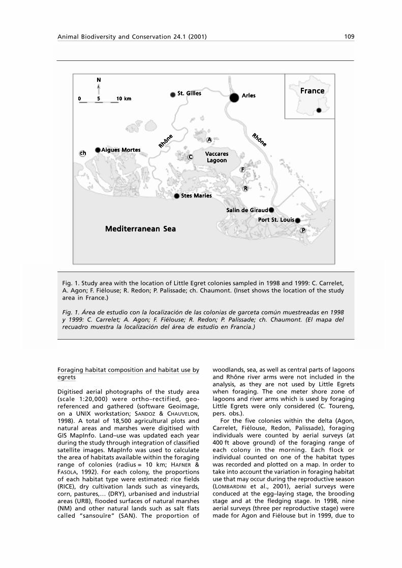
Animal Biodiversity and Conservation 24.1 (2001) 109
Foraging habitat composition and habitat use byegrets
Digitised aerial photographs of the study area(scale 1:20,000) were ortho–rectified, geo-referenced and gathered (software Geoimage,on a UNIX workstation; SANDOZ & CHAUVELON,1998). A total of 18,500 agricultural plots andnatural areas and marshes were digitised withGIS MapInfo. Land–use was updated each yearduring the study through integration of classifiedsatellite images. MapInfo was used to calculatethe area of habitats available within the foragingrange of colonies (radius = 10 km; HAFNER &FASOLA, 1992). For each colony, the proportionsof each habitat type were estimated: rice fields(RICE), dry cultivation lands such as vineyards,corn, pastures,… (DRY), urbanised and industrialareas (URB), flooded surfaces of natural marshes(NM) and other natural lands such as salt flatscalled “sansouïre” (SAN). The proportion of
woodlands, sea, as well as central parts of lagoonsand Rhône river arms were not included in theanalysis, as they are not used by Little Egretswhen foraging. The one meter shore zone oflagoons and river arms which is used by foragingLittle Egrets were only considered (C. Toureng,pers. obs.).
For the five colonies within the delta (Agon,Carrelet, Fiélouse, Redon, Palissade), foragingindividuals were counted by aerial surveys (at400 ft above ground) of the foraging range ofeach colony in the morning. Each flock orindividual counted on one of the habitat typeswas recorded and plotted on a map. In order totake into account the variation in foraging habitatuse that may occur during the reproductive season(LOMBARDINI et al., 2001), aerial surveys wereconduced at the egg–laying stage, the broodingstage and at the fledging stage. In 1998, nineaerial surveys (three per reproductive stage) weremade for Agon and Fiélouse but in 1999, due to
00000 55555 10 km10 km10 km10 km10 km
NNNNN
St. GillesSt. GillesSt. GillesSt. GillesSt. Gilles ArlesArlesArlesArlesArles
Rhône
Rhône
Rhône
Rhône
RhôneAAAAA
CCCCC
FFFFF
RRRRR
PPPPP
Port St. LouisPort St. LouisPort St. LouisPort St. LouisPort St. Louis
Salin de GiraudSalin de GiraudSalin de GiraudSalin de GiraudSalin de Giraud
Stes MariesStes MariesStes MariesStes MariesStes Maries
VVVVVaccaresaccaresaccaresaccaresaccaresLagoonLagoonLagoonLagoonLagoon
chchchchch Aigues MortesAigues MortesAigues MortesAigues MortesAigues Mortes
Mediterranean SeaMediterranean SeaMediterranean SeaMediterranean SeaMediterranean Sea
Rhône
Rhône
Rhône
Rhône
Rhône
FranceFranceFranceFranceFrance
Fig. 1. Study area with the location of Little Egret colonies sampled in 1998 and 1999: C. Carrelet,A. Agon; F. Fiélouse; R. Redon; P. Palissade; ch. Chaumont. (Inset shows the location of the studyarea in France.)
Fig. 1. Área de estudio con la localización de las colonias de garceta común muestreadas en 1998y 1999: C. Carrelet; A. Agon; F. Fiélouse; R. Redon; P. Palissade; ch. Chaumont. (El mapa delrecuadro muestra la localización del área de estudio en Francia.)

110 Tourenq et al.
meteorological and technical hazards and airforceexercises over the study area, were only able toperform eight surveys for Redon, Carrelet andPalissade colonies. Due to flight authorizations(proximity of the Montpellier international civiland Nîmes military airports), we could not carryout aerial survey over the Chaumont colonyforaging range.
Breeding parameters and chicks measurements
For the six colonies, we measured clutch size,brood size and nest success. Little Egrets nestswere individually tagged at the beginning of theseason (early May) and monitored weekly. Theclutch size was defined as the number of eggsper nest after laying was completed. The broodsize was defined as the number of chicksremaining alive at 20–25 days of age for successfulnests. After 20–25 days, chicks are capable ofescaping by walking and may not be present inthe nest (BENNETTS et al., 2000). Nest success wasestimated as the proportion of active nests (i.e.nests with at least one chick) that were successful(i.e. nests that fledged at least one chick).
Measurements included tarsus length (mm),taken from the middle of the mid–tarsal joint tothe distal end of the tarso–metatarsus, and bodymass (g). Chicks were aged according to tarsuslength (THOMAS et al., 1999). All birds werereleased unharmed at the site of capture.
Statistical analysis
Habitat selection by Little Egrets was determinedusing a chi–square goodness–of–fit test tocompare the observed distribution of foragingadults with that expected, relative to theproportion of each suitable habitat availablewithin the foraging range of colonies.
The body condition index (BCI) was calculatedas the residuals from the model II (reducedmajor axis) regression of body mass (W) on thetarsus length (T) (GREEN, 2000). The use ofmodel II regressions is likely more appropriateto study body condition since the use ofresiduals from ordinary least square linearregression of body mass against a linearmeasure of size is subject to errors due tomeasurements and violation of assumptions(SOKAL & ROHLF, 1997; GREEN, 2000).
Clutch size and brood size were comparedbetween colonies using one–way analyses ofvariance (ANOVA) and Tukey–Kramer (HSD)post-hoc tests (SOKAL & ROHLF, 1997). The effectsof habitat types selected by foraging adultLittle Egrets and their interactions on the clutchsize and brood size of egrets for each colonywere assessed using a generalised linear model(GLM) approach. Because the brood size is atleast partially limited by clutch size (HAFNER etal., 2001), the clutch size (CS) was consideredas an explanatory variable of brood size. Little
Egrets nest in mixed colonies with Cattle Egret(Bubulcus ibis), Squacco Heron (Ardeola ralloides),Black–crowned Night Heron (Nycticorax nycticorax)and Grey heron (Ardea cinerea) in the Camargue(TOURENQ et al., 2000). Because of possible density–dependent effects on brood size (BENNETTS et al.,2000; HAFNER et al., 2001), the total number ofbreeding pairs of herons (PAIR) was also consideredas an explanatory variable of brood size. Since1967, all heron colonies have been censused eachyear in the Camargue. The census is based ondirect nest counts and counting error increaseswith colony size, with up to 10% under–estimationof larger colonies, while over–estimation is unlikely(TOURENQ et al., 2000). Using a generalized linearmodel procedure with a identity link function, weexplored the effects of clutch size, total number ofbreeding pairs and habitat types selected byforaging breeding adults on the breedingparameters. Models with non–identifiable or non–estimable effects were ignored. Model selectionwas based on Akaike’s Information Criteria (AICAKAIKE, 1973; SHIBATA, 1989) and multi–modelinference (MMI; ANDERSON et al., 2000). AIC isdefined as:
–2ln(L) + 2npwhere –2ln(L) represents the deviance and np isthe number of parameters estimated in themodel. Models with AIC scores differing by < 2were not considered statistically different(SAKAMOTO et al., 1986).
Multi–model inference is based on the entireset of models, using AIC differences (≅ i ) betweenthe best model, i.e. with the minimum AIC, andeach model and using Akaike weights (∆i;ANDERSON et al., 2000). Akaike weights arecalculated as:
∆i = exp(–0.5≅ i) / ΣRr=1 exp(–0.5≅ i)
where exp (–0.5≅ ι) is the likelihood of a model igiven the data for i = 1, 2,... R models.
Results
Foraging habitat and habitat use
The foraging habitat composition differedsignificantly among the five colonies aerial-surveyed (table 1). The foraging range of theAgon colony mainly consisted of pastures, drycultivation lands (sunflowers) and rice fields. TheFiélouse colony was mainly surrounded by saltflats ("sansouïres") and pastures. The Palissadecolony was located between the industrial saltpans of Salin de Giraud and the industrial zone ofFos–sur–Mer, but near the large natural marshesof they de Roustan and Palissade. The foragingrange of the Redon colony mainly consisted of"sansouïres" from the Vaccarès lagoon system,rice fields, salt pans and some natural marshes.More than 50% of the Carrelet foraging habitatswere natural marshes, the rest being pastures,rice fields and "sansouïres"(table 1).
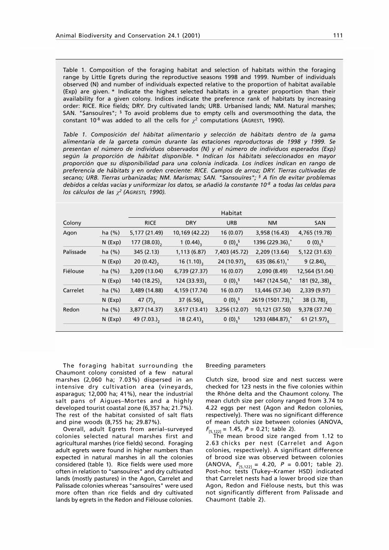
Animal Biodiversity and Conservation 24.1 (2001) 111
The foraging habitat surrounding theChaumont colony consisted of a few naturalmarshes (2,060 ha; 7.03%) dispersed in anintensive dry cultivation area (vineyards,asparagus; 12,000 ha; 41%), near the industrialsalt pans of Aigues–Mortes and a highlydeveloped tourist coastal zone (6,357 ha; 21.7%).The rest of the habitat consisted of salt flatsand pine woods (8,755 ha; 29.87%).
Overall, adult Egrets from aerial–surveyedcolonies selected natural marshes first andagricultural marshes (rice fields) second. Foragingadult egrets were found in higher numbers thanexpected in natural marshes in all the coloniesconsidered (table 1). Rice fields were used moreoften in relation to "sansouïres" and dry cultivatedlands (mostly pastures) in the Agon, Carrelet andPalissade colonies whereas "sansouïres" were usedmore often than rice fields and dry cultivatedlands by egrets in the Redon and Fiélouse colonies.
Breeding parameters
Clutch size, brood size and nest success werechecked for 123 nests in the five colonies withinthe Rhône delta and the Chaumont colony. Themean clutch size per colony ranged from 3.74 to4.22 eggs per nest (Agon and Redon colonies,respectively). There was no significant differenceof mean clutch size between colonies (ANOVA,F[5,122] = 1.45, P = 0.21; table 2).
The mean brood size ranged from 1.12 to2.63 chicks per nest (Carrelet and Agoncolonies, respectively). A significant differenceof brood size was observed between colonies(ANOVA, F[5,122] = 4.20, P = 0.001; table 2).Post–hoc tests (Tukey–Kramer HSD) indicatedthat Carrelet nests had a lower brood size thanAgon, Redon and Fiélouse nests, but this wasnot significantly different from Palissade andChaumont (table 2).
Table 1. Composition of the foraging habitat and selection of habitats within the foragingrange by Little Egrets during the reproductive seasons 1998 and 1999. Number of individualsobserved (N) and number of individuals expected relative to the proportion of habitat available(Exp) are given. * Indicate the highest selected habitats in a greater proportion than theiravailability for a given colony. Indices indicate the preference rank of habitats by increasingorder: RICE. Rice fields; DRY. Dry cultivated lands; URB. Urbanised lands; NM. Natural marshes;SAN. "Sansouïres"; § To avoid problems due to empty cells and oversmoothing the data, theconstant 10-8 was added to all the cells for ✪2 computations (AGRESTI, 1990).
Table 1. Composición del hábitat alimentario y selección de hábitats dentro de la gamaalimentaria de la garceta común durante las estaciones reproductoras de 1998 y 1999. Sepresentan el número de individuos observados (N) y el número de individuos esperados (Exp)según la proporción de hábitat disponible. * Indican los hábitats seleccionados en mayorproporción que su disponibilidad para una colonia indicada. Los índices indican en rango depreferencia de hábitats y en orden creciente: RICE. Campos de arroz; DRY. Tierras cultivadas desecano; URB. Tierras urbanizadas; NM. Marismas; SAN. "Sansouïres"; § A fin de evitar problemasdebidos a celdas vacías y uniformizar los datos, se añadió la constante 10-8 a todas las celdas paralos cálculos de las ✪2 (AGRESTI, 1990).
Habitat
Colony RICE DRY URB NM SAN
Agon ha (%) 5,177 (21.49) 10,169 (42.22) 16 (0.07) 3,958 (16.43) 4,765 (19.78)
N (Exp) 177 (38.03)2 1 (0.44)3 0 (0)4§ 1396 (229.36)1
* 0 (0)5§
Palissade ha (%) 345 (2.13) 1,113 (6.87) 7,403 (45.72) 2,209 (13.64) 5,122 (31.63)
N (Exp) 20 (0.42)2 16 (1.10)3 24 (10.97)4 635 (86.61)1* 9 (2.84)5
Fiélouse ha (%) 3,209 (13.04) 6,739 (27.37) 16 (0.07) 2,090 (8.49) 12,564 (51.04)
N (Exp) 140 (18.25)2 124 (33.93)3 0 (0)5§ 1467 (124.54)1
* 181 (92,.38)4
Carrelet ha (%) 3,489 (14.88) 4,159 (17.74) 16 (0.07) 13,446 (57.34) 2,339 (9.97)
N (Exp) 47 (7)3 37 (6.56)4 0 (0)5§ 2619 (1501.73)1
* 38 (3.78)2
Redon ha (%) 3,877 (14.37) 3,617 (13.41) 3,256 (12.07) 10,121 (37.50) 9,378 (37.74)
N (Exp) 49 (7.03.)2 18 (2.41)3 0 (0)5§ 1293 (484.87)1
* 61 (21.97)4
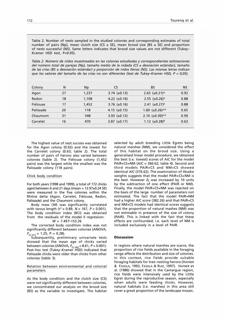
112 Tourenq et al.
The highest value of nest success was obtainedfor the Agon colony (0.92) and the lowest forthe Carrelet colony (0.63; table 2). The totalnumber of pairs of herons also varied betweencolonies (table 2). The Fiélouse colony (1,452pairs) was the largest while the smallest was thePalissade colony (118 pairs).
Chick body condition
For both years (1998 and 1999), a total of 172 chicksaged between 6 and 21 days (mean = 12.97±0.24 SE)were measured in the five colonies within theRhône delta (Agon, Carrelet, Fiélouse, Redon,Palissade) and the Chaumont colony.
Body mass (W) was significantly correlatedwith tarsus length (r2 = 0.89, N = 167, P < 0.001).The body condition index (BCI) was obtainedfrom the residuals of the model II regression:
W = 7.49T–153.26The corrected body condition index was not
significantly different between colonies (ANOVA,F[5,161] = 1.25, P = 0.28).
Subsequently, preliminary univariate testsshowed that the mean age of chicks variedbetween colonies (ANOVA, F[5,166] = 8.61, P < 0.001).Post–hoc test (Tukey–Kramer HSD) indicated thatPalissade chicks were older than chicks from othercolonies (table 3).
Relation between environmental and colonialparameters
As the body condition and the clutch size (CS)were not significantly different between colonies,we concentrated our analysis on the brood size(BS) as the variable to investigate. The habitat
selected by adult breeding Little Egrets beingnatural marshes (NM), we considered the effectof this habitat on the brood size. Using ageneralised linear model procedure, we obtainedthe best (i.e. lowest) scores of AIC for the modelPAIR+CS+NM (AIC = 366.62; table 4). Second andthird models PAIR+CS and NM+CS showedidentical AIC (376.62). The examination of Akaikeweights suggests that the model PAIR+CS+NM isthe best. However ∆i was increased by 10 unitsby the subtraction of one effect (PAIR or NM).Finally, the model PAIR+CS+NM was rejected onthe basis of the large number of parameters notestimated. The fact that the model PAIR+NMhad a higher AIC score (382.26) and that PAIR+CSand NM+CS models had identical scores suggeststhat the proportion of natural mashes (NM) wasnot estimable in presence of the size of colony(PAIR). This is linked with the fact that theseeffects are confounded; i.e. each level of NM isincluded exclusively in a level of PAIR.
Discussion
In regions where natural marshes are scarce, theproportion of rice fields available in the foragingrange affects the distribution and size of colonies.In this context, rice fields provide suitableforaging habitats for tree–nesting herons (HAFNER
& FASOLA, 1992; FASOLA & RUIZ, 1997). HAFNER etal. (1986) showed that in the Camargue region,rice fields were intensively used by the LittleEgret during the reproductive season, especiallywhen adults were feeding chicks. However,natural habitats (i.e. marshes) in this area stillcover a great proportion of the landscape mosaic.
Table 2. Number of nests sampled in the studied colonies and corresponding estimates of totalnumber of pairs (Np), mean clutch size (CS ± SE), mean brood size (BS ± SE) and proportionof nests successful (NS). Same letters indicates that brood size values are not different (Tukey–Kramer HSD test, P<0.05).
Tabla 2. Número de nidos muestreados en las colonias estudiadas y correspondientes estimacionesdel número total de parejas (Np), tamaño medio de la nidada (CS ± desviación estándar), tamañode las crías (BS ± desviación estándar) y porporción de nidos llenos (NS). Las mismas letras indicanque los valores del tamaño de las crías no son diferentes (test de Tukey–Kramer HSD, P < 0,05).
Colony N Np CS BS NS
Agon 27 1,237 3.74 (±0.13) 2.63 (±0.21)a, 0.92
Redon 18 1,108 4.22 (±0.16) 2.55 (±0.26)a 0.88
Fiélouse 17 1,452 3.76 (±0.16) 2.41 (±0.27)a 0.88
Palissade 20 118 4.15 (±0.15) 1.60 (±0.26)a,b 0.65
Chaumont 31 548 3.93 (±0.12) 2.10 (±0.30)a,b 0.90
Carrelet 16 470 3.87 (±0.17) 1.12 (±0.28)b 0.63

Animal Biodiversity and Conservation 24.1 (2001) 113
More recent studies revealed that cultivatedhabitats such as rice fields were avoided (inrelative terms) throughout the year, whereasnatural marshes were the habitat preferred byforaging Litte Egrets (LOMBARDINI et al., 2001). Itwas thus suggested that rice fields might be oflower value than natural marshes.
In this study, aerial surveys revealed that forall monitored colonies, natural marshes werethe habitat preferred (selected more thanexpected regard to its proportion in thelandscape) by adult Little Egrets during thebreeding season, even in an agricultural orindustrial environment. Most natural marshes(about 40% of the Camargue surface area) arepresently situated in protected areas but also inprivate properties devoted to waterfowl hunting(TOURENQ et al., 2000). Thus, valuable foraginghabitats for the Little Egret depend on themaintenance of these natural marshes andwildfowling in the Camargue. Nevertheless, ricefields were the anthropised habitats mostpreferred by egrets. The importance of ricefieldsfor waterbirds may be most pronounced duringextremely dry years when natural marshes aredry. Our study included a relatively dry year(1998, with a total annual rainfall = 471.10 mm)and a relatively wet year (1999, with a total
Table 3. Number of individuals (N), meanage ± SE of Little Egret chicks from thecolonies studied in 1998–1999 in theCamargue, France. Same letters indicatesthat ages are not different (Tukey–KramerHSD test, P < 0.05).
Tabla 3. Número de individuos (N), edadmedia ± desviación estándar de los pollosde las colonias de garceta común estudidasen 1998–1999 en la Camarga francesa. Lasmismas letras indican que las edades noson diferentes (test de Tukey–Kramer HSD,P < 0,05).
Colony N Age (days)
Palissade 21 16.33 (0.66)a
Chaumont 30 13.10 (0.52)b
Fiélouse 12 13.08 (0.53)b
Redon 28 11.21 (0.61)b
Carrelet 49 12.43 (0.44)b
Agon 27 12.48 (0.44)b
Table 4. Modelling the influence of total number of pair of herons (PAIR), clutch size (CS),natural marshes (NM) on the brood size of Little Egrets in the Camargue: Dev. Deviance of themodel; Np. Number of parameters; AIC. Akaike Information Criteria; ≅ i AIC – minAIC; ∆i Akaikeweight; * The model had higher number of estimates non–estimated; (1) Model including two–way interactions; (2) Model including three–way interactions.
Tabla 4. Modelos de influecia del número total de parejas de garzas (PAIR), tamaño de la nidada(CS), marismas (NM) en el tamaño de las crías de garceta común en la Camarga: Dev. Desviacióndel modelo; Np. Número de parámetros; AIC. Criterio de información de Akaike; ≅ i AIC – minAIC;∆i Peso de Akaike; * Modelo con gran número de valores no estimados; (1) Modelo con dos tiposde interacciones; (2) Modelo con tres tipos de interacciones.
Model Dev Np AIC ≅ i ∆i
PAIR+CS+MN* 358,62 4 366,62 0 0.98
CS+MN 358,62 9 376,62 10 0.006
PAIR+CS 358,62 9 376,62 10 0.006
MN 370,26 6 382,26 15,64 0.0001
PAIR 370,26 6 382,26 15,64 0.0001
PAIR+MN 370,26 6 382,26 15,64 0.0001
CS 382,52 4 390,52 23,9 < 0.0001
PAIR/CS/MN∆2*(1) 352,96 20 392,96 26,34 < 0.0001
PAIR/CS/MN∆3*(2) 352,96 20 392,96 26,34 < 0.0001

114 Tourenq et al.
annual rainfall = 719.10 mm) compared to themean annual rainfall of 625.40 mm for the 1963–99 period (Chauvelon, unpub. data). However,colonies surveyed in 1998 (Agon, Fiélouse andChaumont) presented among the highestreproductive performances (see table 2).Moreover, extremely dry years have beenrecorded in the Camargue (e.g., 252.00 mm and325.60 mm for 1989 and 1992, respectively;Chauvelon unpub. data). Our results are thereforeapplicable to a relatively dry year, but do notallow us to extend reliable inference to extremeconditions which may periodically occur.
TIAINEN et al. (1989) suggested that theintensification of farming induced a decrease inthe Finish Starling (Sturnus vulgaris) populationas the result of a reduction in nestling fitness(i.e. growth and survival). In Little Egrets, chickbody condition and reproductive success are saidto be a function of food quality and abundancein the foraging range and of food quantitycollected by adults (HAFNER et al., 1993). Despitethe conversion of many natural marshes into ricefields and other artificial habitats in the past30 years, a general increase in populationnumbers of Little Egrets has been observed inthe Camargue (TOURENQ et al., 2000). The analysisof a series of reproductive parameters in thisspecies revealed no clear stresses in habitats oflittle appeal to egrets. The mean clutch size andchick body condition did not differ betweencolonies. In birds, the number of eggs laid bythe female is partly related to the body conditionof the female before ovulation (e.g. DRENT &DAAN, 1980; MONAGHAN et al., 1989; CHASTEL etal., 1995). However, Little Egrets may be “incomebreeders” (sensu MEIJER & DRENT, 1999) like purpleherons, (Ardea purpurea ; MOSER, 1986): eggs arerelatively small in relation to female body weight(5%, Hafner et al., unpubl. data), thus requiringsmall reserves before their production (MOSER,1986), and both sexes participate in incubationduring laying (HAFNER et al., 1993). Moreover,the Little Egret is a partial migrant (TOURENQ etal., 2000). Thus, females may feed on breedingareas just before and/or during egg production.Further studies are needed to confirm thishypothesis.
Brood size among birds is supposed to reflectlocal conditions (DRENT & DAAN, 1980) and ourresults suggest that brood size may vary with theproportion of natural marshes around colonies.However, we could not separate the effect of theproportion of natural marshes from the effect ofthe colony size. Whereas the Carrelet colony wassurrounded mainly by natural marshes, it wasalso the colony with one of the lowest number ofbreeding pairs, the lowest mean brood size andthe lowest nest success. The brood size of Carreletwas similar to the mean brood size of colonieswith a significant amount of anthropised habitatin their foraging range (Chaumont, Palissade).
One possible stressor not taken into account
in this study could be the ingestion of pesticidesthrough the consumption of food collected inrice fields. Little Egrets are mainly insectivorous–piscivorous (TOURENQ et al., 2000) and non–negligible concentrations of organochlorinepesticides typically used in rice farming weredetected in tissues of fish from the Camargue(ROCHE et al., 2000). Organochlorines were alsofound in the eggs of Little Egrets in colonieswith a «rice environment» (BERNY et al., in press).Through the quality of the food ingested(GRASMAN et al., 1998), contaminants are knownto influence reproductive parameters (NEWTON,1986; BURGER & GOCHFELD, 1991; BERNY et al.,2001). This might also be the case for the Carreletcolony where brood size and nest success werelow. The presence of industrial areas set upstreamand near the mouth of the Rhône river (Fos surMer complex), generates exposure to heavy metalor polychlorinated byphenyls (PCBs) and mayaccount for the presence of contaminants foundin eggs (BATTY et al., 1996; BERNY et al., in press.).This is especially valid for the Palissade colonywhere brood size and nest success were low.Studies are in progress to confirm the impact ofcontaminants on egrets reproduction in theCamargue.
Acknowledgements
We thank the Station Biologique de la Tour duValat, especially H. Hafner and F. Mesléard fortheir support in this study and S. Befeld, A.Berceaux, G. Bertault, R. Cambag, C. Caritey, L.Dami, L. Dietrich, M. Gonzalez, V. Lemoine, A.Mora, and C. Pin for their help in collecting andcompiling the data. We are indebted to B. Blohorn,Mas d’Agon, and J. C. Briffaud, Conservatoire duLittoral–La Palissade, for allowing us to collectdata in their property. We thank A. Besnard,CEFE–CNRS, M. Fasola, University of Pavia (Italy),A. Green, Estación Biológica de Doñana (Spain),and P. Heurteaux for their constructive comments.This study was funded by the Station Biologiquede la Tour du Valat, the Sansouïre Foundation,the MAVA Foundation, and the Centre Françaisdu Riz. The dexterity of the pilots V. Heurteauxand J. Toutain, Aeroclub de Montpellier, was ofgreat value.
References
AEBISCHER, N. J., 1990. Assessing pesticide effectson non–target invertebrates using long–termmonitoring and time–series modelling.Functionary Ecology, 4: 369–373.
AGRESTI, A., 1990. Categorical data analysis. Whiley& Sons, New York.
AKAÏKE, H., 1973. Information theory as anextension of the maximum likelihood principle.In: Second International Symposium on
Animal Biodiversity and Conservation 24.1 (2001) 115
Information Theory: 267–281 (B. N. Petrov & F.Csaki, Eds.). Akademiai Kaido, Budapest,Hungary.
ANDERSON, D. R., BURNHAM, K. P. & THOMPSON, W.L., 2000. Null hypothesis testing: problems,prevalence and an alternative. Journal ofWildlife Management, 64: 912–923.
BATTY, J., PAIN, D. & CAURANT, F., 1996. Metalconcentrations in eels, Anguilla anguilla, fromthe Camargue Region of France. BiologicalConservation, 76: 17–23.
BENNETTS, R. E., FASOLA, M., HAFNER, H. & KAYSER,Y., 2000. Influence of environmental anddensity–dependent factors on reproduction ofLittle Egrets. Auk, 117: 637–639.
BERNY, P., SADOUL, N., DOL, S., VIDEMAN, B., KAYSER,Y. & HAFNER, H. (in press). Impact of localagricultural and industrial practices on eggcontamination of the Little Egret in the Rhônedelta, southern France. EnvironmentalToxicology Chemistry.
BURGER, J. & GOCHFELD, M., 1991. The CommonTern, its breeding biology and social behavior.Columbia University Press, New York.
CARTER, R. V. & ABRAHAMS, M. V., 1997. Predictingthe distribution of organisms among a fewpatches: problems with detecting departuresfrom the ideal free distribution. Oikos, 78:388–393.
CHAMBERLAIN, D. E., WILSON, A. M., BROWNE, S. J. &VICKERY, J. A., 1999. Effects of habitat type andmanagement of skylarks in the breeding season.Journal of Applied Ecology, 36: 856–870.
CHASTEL, O., WEIMERSKIRCH, H. & JOUVENTIN, P.,1995. Boy condition and seabird reproductiveperformance: a study of the petrel species.Ecology, 76: 2240–2246.
CHAUVELON, P., 1996. Hydologie quantitative d’unezone humide méditerranéenne aménagée: lebassin du Fumemorte en Grande Camargue,delta du Rhône. Ph. D. Thesis, Université deMontpellier II.
CLAMENS, A. & ISENMANN, P., 1989. Effect ofsupplemental food on the breeding of Blueand Great Tits in Mediterranean habitats. OrnisScandinavica, 20: 36–42.
DOOLEY, J. L. & BOWERS, M. A., 1998. Demographicresponses to habitat fragmentation: ex–perimental tests at the landscape and patchscale. Ecology, 79: 969–980.
DRENT, R. H. & DAAN, S., 1980. The prudent parent:energetic adjustments in avian breeding.Ardea, 68: 225–252.
FARINA, A., 1997. Landscape structure and breedingbird distribution in a sub–Mediterranean agro–ecosystem. Landscape Ecology, 12: 365–378.
FASOLA, M. & RUIZ, X., 1997. Rice farming andwaterbirds: integrated management in anartificial landscape. In: Farming and Birds inEurope: 210–235 (D. Pain & M. W. Pieckowski,Eds.). Academic Press, London.
GRASMAN, K. A., SCANLON, P. F. & FOX, G. A., 1998.Reproductive and physiological effects of
environmental contaminants in fish–eatingbirds of the Great Lakes: a review of historicaltrends. Environmental Monitoring Assessment,53: 117–145.
GREEN, A. J., 2000. Mass/length residuals: measuresof body condition or generators of spuriousresults? Ecology, 82: 1,473–1,483.
HAFNER, H., BENNETTS, R. E. & KAYSER, Y., 2001,Changes in clutch size, brood size and numbersof nesting Squacco Herons (Ardeola ralloides)over a 32–year period in the Camargue, SouthFrance. Ibis, 143: 11–16.
HAFNER, H., DUGAN, P. J. & BOY, V., 1986. Use ofartificial and natural wetlands as feeding sitesby Little Egrets (Egretta garzetta L.) in theCamargue, southern France. Colonial Water–birds, 9: 149–154.
HAFNER, H., DUGAN, P. J., KERSTEN, M. & WALLACE, J.P., 1993. Flock feeding and food intake inLittle Egrets (Egretta garzetta L.): the effectsof food provisioning on reproductive success.Ibis, 135: 25–32.
HAFNER, H. & FASOLA, M., 1992. The relationshipbetween feeding habitat and colonial nestingArdeidae. In: Managing Mediterranean wetlandsand their birds: 194–201 (C. M. Finlayson, G. E.Hollis & T. J. Davis, Eds.). Proceedings of theSymposium of Grado, Italy, IWRB SpecialPublication 20, Slimbridge, UK.
HEATH, M. F . & EVANS, M. I. (Eds.), 2000. ImportantBird Areas In Europe: Priority Sites forConservation. Vol. 2: Southern Europe. BirdLifeInternational Conservation Series N°8,Cambridge, UK.
LOMBARDINI, K., BENNETTS, R. E. & TOURENQ, C.,2001. Foraging success and foraging habitatuse by Cattle egrets and Little Egrets in theCamargue. Condor, 103: 38–44.
MEIJER, T. & DRENT, R., 1999. Re–examination ofthe capital and income dichotomy in breedingbirds. Ibis, 141: 399–414.
MONAGHAN, P., UTTLEY, J. D., BRUNS, M. D., THAINE, C.& BLACKWOOD, J., 1989. The relationship betweenfood supply, reproductive effort and breedingsuccess in Arctic Terns, Sterna paradisea. Journalof Animal Ecology, 58: 261–274.
MOSER, M. E., 1986. Breeding strategies of purpleherons in the Camargue, France. Ardea, 74:91–100.
NEWTON, I., 1986. The Sparrowhawk. T. & A. D.Poyser, Calton.
PETERSEN, B. S., 1998. The distribution of Danishfarmland birds in relations to habitatscharacteristics. Ornis Fennica, 75: 105–118.
ROCHE, H., BUET, A., JONOT, O. & RAMADE, F., 2000.Organochlorine residues in european eel(Anguilla anguilla), crucian carp (Carassiuscarassius) and catfish (Ictalurus nebulosus) fromVaccares lagoon (French National NatureReserve of Camargue): effects on somephysiological parameters. Aquatic Toxicology,48: 443–459.
SAKAMOTO, Y., ISHIGURO, M. & KITAWAGA, G., 1986.
116 Tourenq et al.
Akaike information criterion statistics. KTKScientific Publishers, Tokyo, Japan.
SANDOZ, A. & CHAUVELON, P., 1998. La géomatiquecomme outil de suivi des conditions hydrolo-giques de la Camargue, zone deltaïque.Méditerranée, 4: 73.
SHIBATA, R., 1989. Statistical aspects of modelselection. In: From data to model: 215–240 (J.C. Willems, Ed.). Springer Verlag, London, UK.
SOKAL, R. R. & ROHLF, F. J., 1997. Biometry. ThirdEdition. Freeman and Co., New York.
STEPHEN, D. W. & KREBS, J. R., 1986. Foragingtheory. Princeton University Press, UK.
THOMAS, F., KAYSER, Y. & HAFNER, H., 1999. Nestlingsize rank in the Little Egret (Egretta garzetta)influences subsequent breeding success ofoffspring. Behavioural Ecology and Socio-biology, 45: 466–470.
TIAINEN, J. T., HANSKI, I. K., PKKALA, T., PIIROINEN, J.& YRJÖLÄ, R., 1989. Clutch size, nestling growthand nestling mortality of the Staling Sturnus
vulgaris in south Finnish agroenvironments.Ornis Fennica, 66: 41–48.
TOURENQ, C., BENNETTS, R. E., KOWALSKI, H., VIALET,E., LUCCHESI, J.–L., KAYSER, Y. & ISENMANN, P. ,2001. Are ricefields a good alternative tonatural marshes for waterbird communities ofthe Camargue, southern France? BiologicalConservation, 100: 335–343.
TOURENQ, C., BENNETTS, R. E., SADOUL, N., MESLEARD,F., KAYSER, Y. & HAFNER, H., 2000. Long-termPopulation and Colony Patterns of Four Speciesof Tree–nesting Herons in the Camargue, SouthFrance. Waterbirds, 23: 236–245.
TUCKER, G. M., 1992. Effects of agriculturalpractices on field use by invertebrate–feedingbirds in winter. Journal of Applied Ecology,29: 779–790.
WILSON, J. D., TAYLOR, R. & MUIRHEAD, L. B., 1996.Field use by farmland birds in winter: ananalysis of field type preferences usingresampling methods. Bird Study, 43: 320–332.

117Animal Biodiversity and Conservation 24.1 (2001)
© 2001 Museu de ZoologiaISSN: 1578–665X
Van Vuren, D. H., 2001. Spatial relations of American bison Bison bison and domestic cattle in a montaneenvironment. Animal Biodiversity and Conservation, 24.1: 117–124.
AbstractAbstractAbstractAbstractAbstractSpatial relations of American bison Bison bison and domestic cattle in a montane environment.— Restorationof American bison (Bison bison) to montane environments where they once occurred requires information onecological relationships with domestic cattle (Bos taurus) that now live there. Comparisons of the foragingdistributions of sympatric bison and cattle in a 375–ha basin revealed that cattle were constrained by slope anddistance from water, especially vertical distance, whereas bison responded mostly to forage availability. Cattleappeared to be central place foragers oriented around water and followed a strategy of meeting their energeticneeds with the least cost. Bison, in contrast, appeared to be energy maximizers that moved often in responseto forage availability. The result was relatively little overlap (29%) in spatial distributions. If bison replace cattlein montane environments, managers can expect a more even distribution of grazing pressure. Bison and cattlemight be managed sympatrically; their spatial distributions may be sufficiently different to minimize competitionfor food, and the risk of interspecific disease transmission as well.
Key words: Bison, Cattle, Foraging Ecology, Montane environments, Spatial relations.
ResumenResumenResumenResumenResumenRelaciones espaciales entre el bisonte americano Bison bison y el ganado vacuno en un medio de montaña.—La reintroducción del bisonte americano (Bison bison) en un ambiente de montaña donde ya había vivido antesrequiere información acerca de las relaciones ecológicas con el ganado vacuno (Bos taurus) que ahora habitaen ese lugar. La comparación de las distribuciones de forrajeo del bisonte con las de la vaca en una cuenca de375 ha demostraron que la vaca estaba limitada por la inclinación del terreno y la distancia al agua,especialmente la distancia vertical, mientras que el bisonte lo estaba principalmente por la disponibilidad depasto. La vaca mostró clara orientación a pacer principalmente alrededor del agua y siguió una estrategia deobtención de sus necesidades energéticas con el mínimo coste. En contraste, el bisonte se mostró maximizadorde energía, efectuando frecuentes desplazamientos en función de la disponibilidad de pastos. El resultado diouna coincidencia relativamente reducida (29%) en las distribuciones espaciales. Si el bisonte sustituye al ganadoen medios de montaña, puede esperarse una mejor distribución de la presión sobre los pastos. Los bisontes yel ganado vacuno pueden convivir en la misma área geográfica, puesto que sus distribuciones espaciales sonsuficientemente diferentes para minimizar la competencia por el alimento, así como el riesgo de transmisióninterespecífica de enfermedades.
Palabras clave: Bisonte, Ganado, Ecología de forrajeo, Medios de montaña, Relaciones espaciales.
(Received: 29 VI 01; Final acceptance: 18 VII 01)
D. H. Van Vuren, Dept. of Wildlife, Fish, and Conservation Biology, Univ. of California, Davis, CA 95616, USA.
Spatial relations ofAmerican bison (Bison bison) anddomestic cattle in amontane environment
D. H. Van Vuren

118 Van Vuren
Introduction
Most grasslands around the world once supportedvast herds of migratory ungulates (FRYXELL et al.,1988; FRANK, et al., 1998). Over the past 150years, however, these herds have been drasticallyreduced by overhunting, and much of theirgrassland habitat has been cultivated for cropsor converted to pasture for domestic livestock(FRYXELL & SINCLAIR, 1988; FRANK et al., 1998).Conservation of remaining herds is threatenedby continued encroachment by an increasinghuman population and conflicts with domesticlivestock (REYNOLDS & HAWLEY, 1987; NORTON–GRIFFITHS, 1995; FRANK et al., 1998).
The American bison, a large migratory ungulatethat was once distributed throughout much ofNorth America, is no exception. Densities weregreatest in the grasslands of the Great Plains,which supported numbers in the tens of millions(ROE, 1970), but bison also lived at lower densitiesin meadows and shrub–steppe communities tothe west, in the Rocky Mountains and in themountains and valleys beyond (ROE, 1970; VAN
VUREN, 1987; MEANEY & VAN VUREN, 1993).Indiscriminate slaughter during the 1800s led tonear–extinction; by 1900, only a few hundredbison remained, almost all of them in captivity.Intensive conservation efforts narrowly avertedextinction, and numbers have recovered to about200,000. Most bison today, however, are intensivelymanaged on private lands for commercial purposesor are confined by fences on wildlife refuges(DARY, 1989; MANNING, 1996). The extensive rangeformerly inhabited by bison has been plowed andconverted to crops or is grazed by domestic cattle.Consequently, bison have recovered from near–extinction, but the ecological role they once playedhas not been restored.
Recent research has demonstrated theecological importance of bison in a variety ofthe biotic communities that they once inhabited(KRUEGER, 1986; FRANK & MCNAUGHTON, 1993;CAMPBELL et al., 1994; KNAPP et al., 1999; STEINAUER
& COLLINS, 2001). Consequently, there has beenincreasing interest in restoring bison to afunctional role in natural areas, both in thegrasslands of the Great Plains and in montaneenvironments to the west (PLUMB & DODD, 1993;WUERTHNER, 1993; CALLENBACH, 1996; HAMILTON,1996; STEPHENSON & FLEENER, 1998; KNAPP et al.,1999). However, domestic cattle, often consideredthe ecological equivalent of bison (NOSS &COOPERRIDER, 1994; HARTNETT et al., 1997;WUERTHNER, 1998), now occupy many of theseareas, raising concerns about the consequencesof restoring bison. If bison and cattle have similarniches and occur in the same area, thencompetition for food may result in managementconflicts (WAGNER, 1978). Further, the possibilityof disease transmission between sympatric bisonand cattle has caused controversy at severallocalities (VAN VUREN & SCOTT, 1995).
Comparisons of bison and cattle in the GreatPlains have revealed interspecific differencesin foraging ecology (PEDEN et al., 1974; PLUMB
& DODD, 1993; HARTNETT et al., 1997), butcorresponding studies have not been done inmontane environments, where abiotic factorsmay be particularly important in influencingforaging distribution. Cattle distribution isstrongly constrained by slope and distancefrom water (MUEGGLER, 1955; ROATH & KRUEGER,1982; GILLEN et al., 1984; GANSKOPP & VAVRA,1987; PINCHAK et al., 1991; TELFER, 1994), andelevation may have an effect as well (SENFT etal., 1983). In contrast, several authors haveclaimed that bison are relatively unaffectedby these factors (WARREN, 1927; FRYXELL, 1928;CAHALANE, 1947; CALLENBACH, 1996), suggestingthe potential for niche differentiat ionbetween bison and cattle. These claims,however, remain unsubstantiated.
The Henry Mountains, a semi–arid range westof the Rocky Mountains, support free–rangingbison and cattle that co–exist in an areacharacterized by rugged topography and limitedwater. Although located about 100 km outside ofthe former range of bison (Van Vuren, unpublisheddata), the Henry Mountains are typical of montaneenvironments where bison are known to haveoccurred (MEANEY & VAN VUREN, 1993). Foragingdistributions of bison and cattle were studied inrelation to slope, distance from water, andelevation. A preliminary analysis suggested thatbison and cattle responded differently to thesefactors (VAN VUREN, 1982). In the present reportthose preliminary findings are confirmed andextended by showing that differential responsesto environmental factors, perhaps stemmingfrom differing evolutionary histories, result inspatial segregation of bison and cattle, withimplications for conservation.
Study area
LLLLLocated in southeastern Utah, USA, the HenryMountains (38o 5’ N, 110o 50’ W) rise abruptlyabove the Colorado Plateau (ca. 1,500 melevation) to 3,540 m elevation at the summit ofMount Ellen, the highest peak. Precipitationincreases with elevation, ranging from 15 cm inthe surrounding deserts of the plateau to > 50 cmon the higher slopes. The lower slopes of therange (ca. 1,800–2,400 m elevation) supportextensive pinyon pine (Pinus edulis) and juniper(Juniperus spp.) woodlands. Slopes above 2,400 mare an interspersion of Douglas fir (Pseudotsugamenziesii), spruce (Picea engelmannnii), and fir(Abies spp.) forests, groves of quaking aspen(Populus tremuloides), and shrub–steppeopenings dominated by shrubs (Artemisia spp.,Symphoricarpos alba), forbs (Penstemon spp.,Oxytropis spp., Astragalus spp.) and perennialgrasses (Poa spp., Festuca spp., Nassella spp.).
Animal Biodiversity and Conservation 24.1 (2001) 119
The highest elevations support subalpinegrasslands dominated by Festuca thurberi andCarex spp.
Bison were introduced to the area in 1941 aspart of early efforts to restore bison and numberedabout 200 at the time of this study (VAN VUREN &BRAY, 1986). The bison were free-ranging andmigrated seasonally, spending summers on theupper slopes of the mountains and moving tolower elevations, mostly to the west andsouthwest, during winter. Domestic cattle havegrazed the Henry Mountains since the late 1800s;the two species were sympatric during summerbut allopatric during winter, when cattle wereherded to ranges apart from bison.
The study area comprised the 375–ha basinthat formed the headwaters of South Creek,which drained the west side of Mount Ellen.Elevation ranged from 2,800 m on the west sideof the basin to 3,400 m at the head. Slopes weregentle in much of the central and western portionof the basin but increased steadily toward theeast, reaching 40o at the head of the basin.Vegetation in the lower portion of the basinconsisted of conifer or aspen groves interspersedwith shrub-steppe openings, the middle portionwas mostly shrub–steppe, and the upper portionsupported subalpine grassland. Both bison andcattle frequently grazed the basin during thestudy; about 30 cattle lived there all summer,and groups of up to 60 bison were often present.Drinking water was available all summer at sevensprings and catchment basins. There were nofences, and cattle were not herded after beingmoved into the basin during late spring; thus,the entire basin was physically accessible to bothspecies.
Methods
The study was conducted July and August 1977and June through September 1978. Spatialdistributions were determined visually; bison andcattle were observed and classified as foraging ornot, and their locations were plotted at 30–minuteintervals on a 1:24,000 topographic map of thebasin. The map was overlaid with a grid scaledat 100–m intervals (thus, 1 ha per grid cell), andeach observation was assigned to the grid cellthat it fell within. Bison and cattle were observedfrom several vantage points, none of whichallowed a view of the entire basin, so vantagepoints were rotated among to ensure that allparts of the basin were surveyed. Observationswere distributed throughout daylight hours.
The numbers of observations of foraging bisonand cattle were summed for each grid cell.Environmental factors were measured at thecenter of each grid cell. A clinometer was usedto measure slope and a topographic map wasused to determine elevation and distance fromthe nearest source of drinking water; horizontal
and vertical distance from water were recordedas separate factors. Frequency distributions wereused to compare the spatial distributions of bisonand cattle in relation to each environmentalfactor. The range of each factor was divided intointervals and all observations of bison or cattlethat fell within each interval for slope(4o intervals), horizontal (100–m intervals) andvertical (30–m intervals) distance from water,and elevation (50–m intervals) were totaled.Frequency distributions of bison and cattle werecompared using a G–test of independence.Observations were not independent, but this is aconcern only if analyses yield marginallysignificant results, which did not happen. Tocompare the spatial distributions of bison andcattle graphically a three–dimensional mesh plotwas used, in which x– and y–coordinatescorresponded to the axes of the grid that overlaythe basin, and the z–coordinate represented thefrequency of use of each grid cell. To comparespatial distributions numerically, Kulczynski’ssimilarity index was calculated (OOSTING, 1956),which compares frequencies in each grid square,then sums for all grid squares. The index rangesfrom 0 (completely different use of space) to1 (identical use of space).
The foraging distribution of cattle oftendeclines exponentially with increasing distancefrom water (MUEGGLER, 1955; ROATH & KRUEGER,1982; NASH et al., 1999), creating a “piosphere”,a zone of attenuating impact away from eachwatering point (ANDREW, 1988). A similarexponential decline may exist with increasingslope (GANSKOPP & VAVRA, 1987). This relationshipwas evaluated for bison and for cattle byregressing the square root of proportion ofobservations on each of three variables,horizontal distance from water, vertical distancefrom water, and slope. Because only a negativerelationship was expected, one–tailed tests wereused.
Results
Among > 22,000 observations of bison and >3,000of cattle recorded in the study area, 9745 were offoraging bison and 1,196 were of foraging cattle.The species differed markedly in the slopes theygrazed (G = 1,264.0, P < 0.001); cattle occurrencedeclined rapidly as slope increased beyond 4o,whereas bison exhibited a bimodal pattern withthe highest peak in occurrence at 28–32o (fig. 1).Cattle observations fit a negative exponentialrelationship with slope (r2 = 0.86, P < 0.001), butbison observations did not (r2 = 0.03, P > 0.50).
The species were less differentiated accordingto horizontal distance from water, yet differenceswere evident (G = 492.0, P < 0.001). Cattleoccurrence declined with increasing distance,while bison occurrence was unrelated to distanceuntil beyond 700 m. Cattle observations fit a
120 Van Vuren
negative exponential relationship with horizontaldistance from water (r2 = 0.88, P < 0.001); so didbison observations, but the fit was poor (r2 = 0.33,P = 0.04) and the slope was less negative thanthat of cattle (t = 2.53, P < 0.05).
The species differed strikingly according tovertical distance from water (G = 1,260.7,P < 0.001). Cattle occurrence declined steeply withincreasing distance, whereas bison occurrencedecreased only slightly. Cattle observations fit anegative exponential relationship with verticaldistance from water (r2 = 0.78, P < 0.001); thedecline was so steep, however, that examinationof the residuals indicated a fourth–roottransformation was a better representation ofthe relationship (r2 = 0.83, P < 0.001). Bisonobservations also fit a negative exponentialrelationship (r2 = 0.72, P < 0.001), but the slopewas less negative than that of cattle (t = 2.75,P < 0.02).
Bison and cattle differed in the elevationsthey grazed (G = 1,354.0, P < 0.001), with bisongrazing more often at higher elevations.
The spatial distributions of bison and cattle inthe basin were not uniform, in part becauseboth species grazed almost entirely in shrub-steppe or subalpine grassland communities andused conifer or aspen groves mostly for resting.However, within shrub–steppe and grasslandcommunities, differential response of bison andcattle to slope, distance from water, and elevationtranslated into differential use of space. Bisonand cattle were recorded in similar numbers ofgrid squares (163 and 16, respectively), but only66 grid squares were grazed by both species.Intensity of use differed as well. Two pronouncedpeaks in cattle distribution, in the north andnorthwest portions of the basin, occurred atlarge “flats” with level or gentle slopes anddrinking water nearby (fig. 2). Most of the lesserpeaks in cattle occurrence were located at smallerflats with adjacent water. Some bison also grazedthese areas, but most bison observations weredistributed in an arc that extended across thehighest (and steepest) slopes at the head of thebasin and along the north slope of the ridge thatformed the southern boundary of the basin(fig. 2). Graphical differences in distribution weresupported numerically; the similarity index wasonly 0.286, indicating that spatial distributionsof foraging bison and cattle were largelydissimilar.
Discussion
Distribution of cattle was strongly constrainedby slope, although not as severely as in otherstudies, which reported that cattle seldom usedslopes greater than 11o (GILLEN et al., 1984;GANSKOPP & VAVRA, 1987; PINCHAK et al., 1991;TELFER, 1994). Bison, in contrast, frequented muchsteeper slopes than did cattle, both in the Henry
Mountains and elsewhere, exhibiting a peak indistribution at about 30o and confirming earlierassertions (FRYXELL, 1928). Horizontal distancefrom water seemed less important to cattledistribution than did slope, probably because allparts of the basin were relatively close to water(< 1000 m) and because response of cattle toproximity of water is influenced by other factors,especially topography (HOLECHEK et al., 1989).Nonetheless, bison were relatively unaffected byavailability of water compared with cattle andin particular were less likely to graze close towater, again confirming previous claims(CAHALANE, 1947; CALLENBACH, 1996). In contrastto horizontal distance from water, verticaldistance from water sharply constrained cattledistribution. These findings parallel those ofROATH & KRUEGER (1982), who found that cattlerarely grazed sites more than 80 m above water.Bison were much less affected than cattle byvertical distance from water.
Bison grazed at higher elevations than cattle;however, they probably were responding toforage availability rather than elevation.Precipitation in the Henry Mountains increaseslinearly with elevation (VAN VUREN & BRAY, 1986),and so does forage availability; production ofgraminoids, the primary food of both bison andcattle (VAN VUREN, 1984), ranged 31–179 kg/ha(dry basis) in the study area and increased withelevation (r = 0.85, P < 0.05; Van Vuren,unpublished data). This gradient may have beenexacerbated by depletion of forage at lowerelevations by cattle concentrated on gentle slopesnear water (ANDREW, 1988; HOLECHEK et al., 1989).These findings agree with those from the GreatPlains, where availability of graminoids was amore important factor for bison than cattle indetermining foraging distribution (PLUMB & DODD,1993).
Thus, these results suggest that slope anddistance from water, especially vertical distance,are most important in influencing cattledistribution, whereas availability of forage ismore important for bison. The result was littlespatial overlap between the species. Analternative explanation, that spatial segregationresulted from behavioral avoidance, is unlikely;the species sometimes grazed close to each other,and neither species altered its behavior inresponse to the other until about 4 m apart,whereupon cattle always avoided bison (VAN
VUREN, 1980).Bison and cattle are closely related and are
generally similar in size, appearance, and foodpreference (WUERTHNER, 1998), consequently theirdiffering spatial distributions are somewhatsurprising. Perhaps the explanation lies in theirdiffering evolutionary histories. Cattle originatedin mesic environments of Eurasia whereas bisonevolved in the semi–arid Great Plains, consequent-ly cattle may have a greater requirement forwater (NOSS & COOPERRIDER, 1994; WUERTHNER,
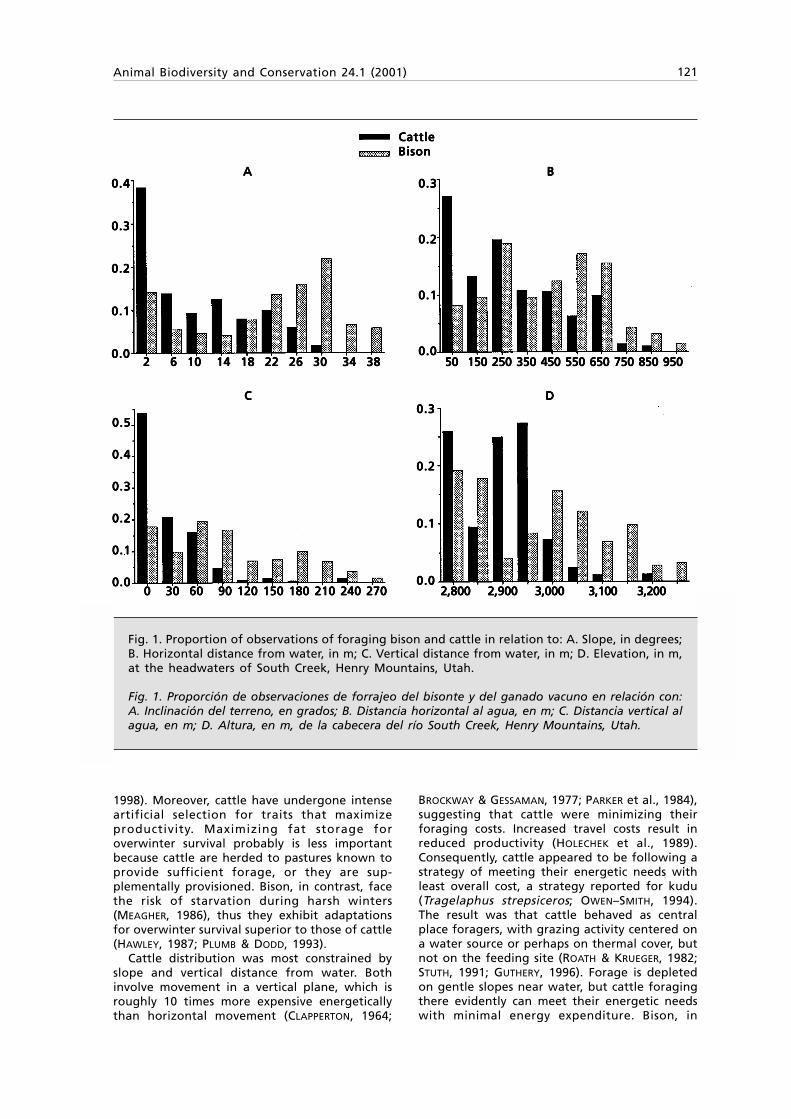
Animal Biodiversity and Conservation 24.1 (2001) 121
1998). Moreover, cattle have undergone intenseartificial selection for traits that maximizeproductivity. Maximizing fat storage foroverwinter survival probably is less importantbecause cattle are herded to pastures known toprovide sufficient forage, or they are sup-plementally provisioned. Bison, in contrast, facethe risk of starvation during harsh winters(MEAGHER, 1986), thus they exhibit adaptationsfor overwinter survival superior to those of cattle(HAWLEY, 1987; PLUMB & DODD, 1993).
Cattle distribution was most constrained byslope and vertical distance from water. Bothinvolve movement in a vertical plane, which isroughly 10 times more expensive energeticallythan horizontal movement (CLAPPERTON, 1964;
BROCKWAY & GESSAMAN, 1977; PARKER et al., 1984),suggesting that cattle were minimizing theirforaging costs. Increased travel costs result inreduced productivity (HOLECHEK et al., 1989).Consequently, cattle appeared to be following astrategy of meeting their energetic needs withleast overall cost, a strategy reported for kudu(Tragelaphus strepsiceros; OWEN–SMITH, 1994).The result was that cattle behaved as centralplace foragers, with grazing activity centered ona water source or perhaps on thermal cover, butnot on the feeding site (ROATH & KRUEGER, 1982;STUTH, 1991; GUTHERY, 1996). Forage is depletedon gentle slopes near water, but cattle foragingthere evidently can meet their energetic needswith minimal energy expenditure. Bison, in
CattleCattleCattleCattleCattleBisonBisonBisonBisonBison
Fig. 1. Proportion of observations of foraging bison and cattle in relation to: A. Slope, in degrees;B. Horizontal distance from water, in m; C. Vertical distance from water, in m; D. Elevation, in m,at the headwaters of South Creek, Henry Mountains, Utah.
Fig. 1. Proporción de observaciones de forrajeo del bisonte y del ganado vacuno en relación con:A. Inclinación del terreno, en grados; B. Distancia horizontal al agua, en m; C. Distancia vertical alagua, en m; D. Altura, en m, de la cabecera del río South Creek, Henry Mountains, Utah.
AAAAA BBBBB
CCCCC DDDDD
0.40.40.40.40.4
0.30.30.30.30.3
0.20.20.20.20.2
0.10.10.10.10.1
0.00.00.00.00.0
0.30.30.30.30.3
0.20.20.20.20.2
0.10.10.10.10.1
0.00.00.00.00.0
0.50.50.50.50.5
0.40.40.40.40.4
0.30.30.30.30.3
0.20.20.20.20.2
0.10.10.10.10.1
0.00.00.00.00.0
0.30.30.30.30.3
0.20.20.20.20.2
0.10.10.10.10.1
0.00.00.00.00.0
2 6 10 14 18 22 26 30 34 38 2 6 10 14 18 22 26 30 34 38 2 6 10 14 18 22 26 30 34 38 2 6 10 14 18 22 26 30 34 38 2 6 10 14 18 22 26 30 34 38 50 150 250 350 450 550 650 750 850 95050 150 250 350 450 550 650 750 850 95050 150 250 350 450 550 650 750 850 95050 150 250 350 450 550 650 750 850 95050 150 250 350 450 550 650 750 850 950
0 30 60 90 120 150 180 210 240 2700 30 60 90 120 150 180 210 240 2700 30 60 90 120 150 180 210 240 2700 30 60 90 120 150 180 210 240 2700 30 60 90 120 150 180 210 240 270 2,8002,8002,8002,8002,800 2,9002,9002,9002,9002,900 3,0003,0003,0003,0003,000 3,1003,1003,1003,1003,100 3,2003,2003,2003,2003,200

122 Van Vuren
Fig. 2. Three–dimensional mesh plots of the foraging distributions of bison and cattle at theheadwaters of South Creek, Henry Mountains, Utah. The z–coordinate indicates frequency ofoccurrence in each grid square. Slope and elevation increase from west to east, and watersources are denoted by black circles.
Fig. 2. Gráfico en malla tridimensional de la distribución de pasto del bisonte y del ganadovacuno en las cabeceras del río South Creek, Henry Mountains, Utah. La coordenada z indica lafrecuencia de forrajeo en cada cuadrícula. La inclinación y la altura aumentan de oeste a este,las fuentes de agua se indican con círculos negros.
WWWWWestestestestest
South
South
South
South
South
CattleCattleCattleCattleCattle
BisonBisonBisonBisonBison
contrast, behaved as energy maximizers, willingto expend energy to obtain richer rewards, withgrazing activity oriented on the feeding siterather than on a water source. Bison typicallyrested within or adjacent to the feeding site,traveled once per day to water and drank briefly
(x = 21 minutes), then returned to the feedingsite or moved to a new one (VAN VUREN, 1980).Bison moved much more than cattle; most cattleremained within the 375–ha basin throughoutthe summer, whereas bison roamed about homeranges that averaged 5,220 ha (VAN VUREN, 1983),

Animal Biodiversity and Conservation 24.1 (2001) 123
rarely remaining in the same area longer than3 days (VAN VUREN, 1980).
Spatial segregation of sympatric bison andcattle on montane ranges during summer,resulting from differential response to environ-mental factors, has important implications forconservation. If bison replace cattle, managerscan expect a more even distribution of grazingpressure in response to forage availability, withlittle evidence of a piosphere, instead of aclumped distribution in response to slope anddistance from water.
Bison and cattle might even be managedsympatrically; although their diets are generallysimilar, their spatial distributions may be sufficientlydifferent not only to minimize competition forfood, but also to reduce the risk of transmission ofdiseases requiring close spatial proximity.
Acknowledgments
I thank the U. S. Bureau of Land Management,Utah Division of Wildlife Resources, Mzuri SafariFoundation, and Sigma Xi for financial andlogistical support; Marty Bray, Bruce Coblentz,and Golden and Keith Durfey for assistancethroughout the study; and Vickie Bakker, ChrisFloyd and Rob Klinger for helpful comments onthe manuscript.
References
ANDREW, M. H., 1988. Grazing impact in relationto livestock watering points. Trends Ecol. &Evol., 3: 336–339.
BROCKWAY, J. M. & GESSAMAN, J. A., 1977. Theenergy cost of locomotion on the level and ongradients for the red deer (Cervus elaphus).Quart. J. Exp. Physiol., 62: 333–339.
CAHALANE, V. H., 1947. Mammals of NorthAmerica. MacMillan Company, New York.
CALLENBACH, E., 1996. Bring back the buffalo!Island Press, Washington, DC.
CAMPBELL, C., BLYTH, C. B. & MCANDREWS, J. H.,1994. Bison extirpation may have caused aspenexpansion in western Canada. Ecography, 17:360–362.
CLAPPERTON, J. L., 1964. The energy metabolismof sheep walking on the level and on gradients.Brit. J. Nutr., 18: 47–54.
DARY, D. A., 1989. The buffalo book. SwallowPress/Ohio University Press, Athens, Ohio.
FRANK, D. A. & MCNAUGHTON, S. J., 1993. Evidencefor the promotion of aboveground grasslandproduction by native large herbivores inYellowstone National Park. Oecologia, 96:157–161.
FRANK, D. A., MCNAUGHTON, S. J. & TRACY, B. F.,1998. The ecology of the Earth’s grazingecosystems. Bioscience, 48: 513–521.
FRYXELL, F. M., 1928. The former range of the
bison in the Rocky Mountains. J. Mammal., 9:129–139.
FRYXELL, J. M., GREEVER, J. & SINCLAIR, A. R. E.,1988. Why are migratory ungulates soabundant? Am. Nat., 131: 781–798.
FRYXELL, J. M. & SINCLAIR, A. R. E., 1988. Causesand consequences of migration by largeherbivores. Trends Ecol. & Evol., 3: 237–241.
GANSKOPP, D. & VAVRA, M., 1987. Slope use bycattle, feral horses, deer, and bighorn sheep.Northwest Sci., 61: 74–81.
GILLEN, R. L., KRUEGER, W. C. & MILLER, R. F., 1984.Cattle distribution on mountain rangeland innorthwestern Oregon. J. Range Manage., 37:549–553.
GUTHERY, F. S., 1996. Upland gamebirds. In:Rangeland wildlife: 59–69 (P. R. Krausman,Ed.). Society for Range Management, Denver.
HAMILTON, R. G., 1996. Using fire and bison to restorea functional tallgrass prairie landscape. Trans. N.Am. Wildl. & Nat. Resour. Conf., 61: 208–214.
HARTNETT, D. C., STEUTER, A. A. & HICKMAN, K. R.,1997. Comparative ecology of native andintroduced ungulates. In: Ecology andconservation of Great Plains vertebrates: 72–101 (F. L. Knopf & F. B. Samson, Eds.). Springer–Verlag, New York.
HAWLEY, A. W. L., 1987. Bison and cattle use offorages. In: Bison ecology in relation toagricultural development in the Slave Riverlowlands, NWT. Occasional Paper 63,: 49–52(H. W. Reynolds & A. W. L. Hawley, Eds.).Canadian Wildlife Service, Edmonton.
HOLECHEK, J. L., PIEPER, R. D. & HERBEL, C. H.,1989. Range management. Prentice Hall,Englewood Cliffs.
KNAPP, A. K., BLAIR, J. M., BRIGGS, J. M., COLLINS,S. L., HARTNETT, D. C., JOHNSON, L. C. & TOWNE,E. G., 1999. The keystone role of bison inNorth American tallgrass prairie. Bioscience,49: 39–50.
KRUEGER, K., 1986. Feeding relationships amongbison, pronghorn, and prairie dogs: anexperimental analysis. Ecology, 67: 760–770.
MANNING, R., 1996. The buffalo is coming back.Defenders, 71(1): 6–15.
MEAGHER, M. M., 1986. Bison bison. Mammal.Spec., 266: 1–8.
MEANEY, C. A. & VAN VUREN, D., 1993. Recentdistribution of bison in Colorado west of theGreat Plains. Proc. Denver Mus. Nat. Hist., 3(4):1–10.
MUEGGLER, W. F., 1955. Cattle distribution onsteep slopes. J. Range Manage., 18: 255–257.
NASH, M. S, WHITFORD, W. G., DE SOYZA, A. G., VAN
ZEE, J. W. & HAVSTAD, K. M., 1999. Livestockactivity and Chihuahuan Desert annual–plantcommunities: boundary analysis of disturbancegradients. Ecol. Applic., 9: 814–823.
NOSS, R. F. & COOPERRIDER, A. Y., 1994. Savingnature’s legacy. Island Press, Washington, DC.
NORTON–GRIFFITHS, M., 1995. Economic incentivesto develop the rangelands of the Serengeti:
124 Van Vuren
implications for wildlife conservation. In:Serengeti II: dynamics, management andconservation of an ecosystem: 588–604 (A. R.E. Sinclair & P. Arcese, Eds.). University ofChicago Press, Chicago.
OOSTING, H. J., 1956. The study of plant communities,2nd ed. W. H. Freeman, San Francisco.
OWEN–SMITH, O., 1994. Foraging responses of kudusto seasonal changes in food resources: elasticityin constraints. Ecology, 75: 1,050–1,062.
PARKER, K. L., ROBBINS, C. T. & HANLEY, T. A., 1984.Energy expenditures for locomotion by muledeer and elk. J. Wildl. Manage., 48: 474–488.
PEDEN, D. G., VAN DYNE, G. M., RICE, R. W. &HANSEN, R. M., 1974. The trophic ecology ofBison bison L. on shortgrass plains. J. Appl.Ecol., 11: 489–497.
PINCHAK, W. E., SMITH, M. A., HART, R. H. &WAGGONER, J. W. JR., 1991. Beef cattledistribution patterns on foothill range. J.Range Manage., 44: 267–275.
PLUMB, G. E. & DODD, J. L., 1993. Foraging ecologyof bison and cattle on a mixed prairie:implications for natural area management.Ecol. Applic., 3: 631–643.
REYNOLDS, H. W. & HAWLEY, A. W. L., 1987.Introduction. In: Bison ecology in relation toagricultural development in the Slave Riverlowlands, NWT, Occasional Paper 63: 10–12(H. W. Reynolds & A. W. L. Hawley, Eds.).Canadian Wildlife Service, Edmonton.
ROATH, L. R. & KRUEGER, W. C., 1982. Cattle grazingand behavior on a forested range. J. RangeManage., 35: 332–338.
ROE, F. G., 1970. The North American buffalo, 2nd
ed. University of Toronto Press, Toronto.SENFT, R. L., RITTENHOUSE, L. R. & WOODMANSEE, R.
G., 1983. The use of regression models topredict spatial patterns of cattle behavior. J.Range Manage., 36: 553–557.
STEINAUER, E. M. & COLLINS, S. L., 2001. Feedbackloops in ecological hierarchies following urinedeposition in tallgrass prairie. Ecology, 82:1,319–1,329.
STEPHENSON, R. O. & FLEENER, C. L., 1998. Bio-political perspectives on a proposed wood bisonreintroduction to Alaska. In: International
symposium on bison ecology and managementin North America: 251–257 (L. Irby & J. Knight,Eds.). Montana State University, Bozeman.
STUTH, J. W., 1991. Foraging behavior. In: Grazingmanagement: 65–83 (R. K. Heitschmidt & J. W.Stuth, Eds.). Timber Press, Portland.
TELFER, E. S., 1994. Cattle and cervid interactionson a foothills watershed in southwesternAlberta. Can. Field–Nat., 108: 186–194.
VAN VUREN, D., 1980. Ecology and behavior ofbison in the Henry Mountains, Utah. M. S.Thesis, Oregon State University.
– 1982. Comparative ecology of bison and cattlein the Henry Mountains, Utah. In: Proceedingsof the wildlife–livestock relationships sym-posium: 449–457 (J. M. Peek & P. D. Dalke,Eds.). University of Idaho Forestry, Wildlife &Range Experiment Station, Moscow, Idaho.
– 1983. Group dynamics and summer homerange of bison in southern Utah. J. Mammal.,64: 329–332.
– 1984. Summer diets of bison and cattle insouthern Utah. J. Range Manage., 37: 260–261.
– 1987. Bison west of the Rocky Mountains: analternative explanation. Northwest Sci., 61:65–69.
VAN VUREN, D. & BRAY, M. P., 1986. Populationdynamics of bison in the Henry Mountains,Utah. J. Mammal., 67: 503–511.
VAN VUREN, D. & SCOTT, C. A., 1995. Internalparasites of sympatric bison, Bison bison,and cattle, Bos taurus. Can. Field–Nat., 109:467–469.
WAGNER, F. H., 1978. Livestock grazing and thelivestock industry. In: Wildlife and America:121–145 (H. P. Brokaw, Ed.). Council onEnvironmental Quality, Washington, DC.
WARREN, E. R., 1927. Altitude limit of bison. J.Mammal., 8: 60–61.
WUERTHNER, G., 1993. Envisioning wildlandrestoration. Wild Earth, 3(3): 70–74.
– 1998. Are cows just domestic bison? Behavioraland habitat use differences between cattleand bison. In: International symposium onbison ecology and management in NorthAmerica: 374–383 (L. Irby & J. Knight, Eds.).Montana State University, Bozeman.

Animal Biodiversity and Conservation 24.1 (2001) I
ISSN: 1578–665X © 2001 Museu de Zoologia
Animal Biodiversity and Conservation
Animal Biodiversity and ConservationAnimal Biodiversity and ConservationAnimal Biodiversity and ConservationAnimal Biodiversity and ConservationAnimal Biodiversity and Conservation (abansMiscel·lània ZoològicaMiscel·lània ZoològicaMiscel·lània ZoològicaMiscel·lània ZoològicaMiscel·lània Zoològica) és una revista inter-disciplinària publicada, des de 1958, pel Museude Zoologia de Barcelona. Inclou articlesd'investigació empírica i teòrica en totes les àreesde la zoologia (sistemàtica, taxonomia, morfo-logia, biogeografia, ecologia, etologia, fisiologiai genètica) procedents de totes les regions delmón, amb especial énfasis als estudis que d'unamanera o altre tinguin relevància en la biologíade la conservació. La revista no publica catàlegs,llistes d'espècies o cites puntuals. Els estudisrealitzats amb espècies rares o protegides podenno ser acceptats tret que els autors disposin delspermisos corresponents. Cada volum anual cons-ta de dos fascicles.
Animal Biodiversity and ConservationAnimal Biodiversity and ConservationAnimal Biodiversity and ConservationAnimal Biodiversity and ConservationAnimal Biodiversity and Conservation es trobaregistrada en la majoria de les bases de dadesmés importants, de manera que permet una difusiómundial dels seus articles.
Tots els manuscrits són revisats per l'editor executiu,un editor i dos revisors independents, triats d'unallista internacional, a fi de garantir-ne la qualitat. Elprocés de revisió és ràpid i constructiu. La publicaciódels treballs acceptats es fa normalment dintre dels12 mesos posteriors a la recepció.
Una vegada hagin estat acceptats passaran aser propietat de la revista. Aquesta es reserva elsdrets d’autor, i cap part dels treballs no podràser reproduïda sense citar–ne la procedència.
Normes de publicació
Els treballs s'enviaran preferentment de formaelectrònica ([email protected]). El formatpreferit és un document Rich Text Format (RTF) oDOC que inclogui les figures (TIF). Si s'opta per laversió impresa, s'han d'enviar quatre còpies deltreball juntament amb una còpia en disquet a laSecretaria de Redacció. Cal incloure, juntamentamb l'article, una carta on es faci constar que eltreball està basat en investigacions originals nopublicades anteriorment i que està sotmès a Ani-Ani-Ani-Ani-Ani-mal Biodiversity and Conservationmal Biodiversity and Conservationmal Biodiversity and Conservationmal Biodiversity and Conservationmal Biodiversity and Conservation en exclusiva.A la carta també ha de constar, per a aquellstreballs en que calgui manipular animals, que elsautors disposen dels permisos necessaris i quecompleixen la normativa de protecció animalvigent. També es poden suggerir possibles assessors.
Quan l'article sigui acceptat, els autors haurand'enviar a la Redacció una còpia impresa de laversió final acompanyada d'un disquet indicantel programa utilitzat (preferiblement en Word).Les proves d'impremta enviades a l'autor per ala correcció, seran retornades al Consell Editoren el termini de 10 dies. Aniran a càrrec delsautors les despeses degudes a modificacionssubstancials introduïdes per ells en el text origi-nal acceptat.
El primer autor rebrà 50 separates del treballsense càrrec a més d'una separata electrònica enformat PDF.
Manuscrits
Els treballs seran presentats en format DIN A–4(30 línies de 70 espais cada una) a doble espai iamb totes les pàgines numerades. Els manuscritshan de ser complets, amb taules i figures. Nos'han d'enviar les figures originals fins quel'article no hagi estat acceptat.
El text es podrà redactar en anglès, castellà ocatalà. Se suggereix als autors que enviïn els seustreballs en anglès. La revista els ofereix, sensecap càrrec, un servei de correcció per part d'unapersona especialitzada en revistes científiques.En tots els casos, els textos hauran de ser redactatscorrectament i amb un llenguatge clar i concís.La redacció del text serà impersonal, i s'evitaràsempre la primera persona.
Els caràcters cursius s’empraran per als nomscientífics de gèneres i d’espècies i per alsneologismes intraduïbles; les cites textuals,independentment de la llengua, seran consignadesen lletra rodona i entre cometes i els noms d’autorque segueixin un tàxon aniran en rodona.
Quan se citi una espècie per primera vegadaen el text, es ressenyarà, sempre que siguipossible, el seu nom comú.
Els topònims s’escriuran o bé en la formaoriginal o bé en la llengua en què estigui escritel treball, seguint sempre el mateix criteri.
Els nombres de l’u al nou, sempre que estiguinen el text, s’escriuran amb lletres, excepte quanprecedeixin una unitat de mesura. Els nombresmés grans s'escriuran amb xifres excepte quancomencin una frase.
Les dates s’indicaran de la forma següent:28 VI 99; 28, 30 VI 99 (dies 28 i 30); 28-30 VI 99(dies 28 a 30).
S’evitaran sempre les notes a peu de pàgina.
Format dels articles
TítolTítolTítolTítolTítol..... El títol serà concís, però suficientmentindicador del contingut. Els títols amb desig-nacions de sèries numèriques (I, II, III,...) seranacceptats previ acord amb l'editor.Nom de l’autor o els autors.Nom de l’autor o els autors.Nom de l’autor o els autors.Nom de l’autor o els autors.Nom de l’autor o els autors.AbstractAbstractAbstractAbstractAbstract en anglès que no ultrapassi les 12 líniesmecanografiades (860 espais) i que mostril’essència del manuscrit (introducció, material,mètodes, resultats i discussió). S'evitaran lesespeculacions i les cites bibliogràfiques. Estaràencapçalat pel títol del treball en cursiva.Key wordsKey wordsKey wordsKey wordsKey words en anglès (sis com a màxim), queorientin sobre el contingut del treball en ordred’importància.ResumenResumenResumenResumenResumen en castellà, traducció de l'Abstract. Dela traducció se'n farà càrrec la revista per aaquells autors que no siguin castellanoparlants.Palabras clave Palabras clave Palabras clave Palabras clave Palabras clave en castellà.

II
Adreça postalAdreça postalAdreça postalAdreça postalAdreça postal de l’autor o autors.(Títol, Nom, Abstract, Key words, Resumen, Pala-bras clave i Adreça postal, conformaran la pri-mera pàgina.)
Introducción. Introducción. Introducción. Introducción. Introducción. S'hi donarà una idea dels antecedentsdel tema tractat, així com dels objectius del treball.Material y métodosMaterial y métodosMaterial y métodosMaterial y métodosMaterial y métodos..... Inclourà la informaciópertinent de les espècies estudiades, aparellsemprats, mètodes d’estudi i d’anàlisi de les dadesi zona d’estudi.ResultadosResultadosResultadosResultadosResultados..... En aquesta secció es presentaranúnicament les dades obtingudes que no haginestat publicades prèviament.DiscusiónDiscusiónDiscusiónDiscusiónDiscusión..... Es discutiran els resultats i es compa-raran amb treballs relacionats. Els suggerimentsde recerques futures es podran incloure al finald’aquest apartat.AgraAgraAgraAgraAgradecimientosdecimientosdecimientosdecimientosdecimientos (optatiu).ReferReferReferReferReferencencencencenciiiiiaaaaasssss..... Cada treball haurà d’anar acompanyatde les referències bibliogràfiques citades en eltext. Les referències han de presentar–se segonsels models següents (mètode Harvard):* Articles de revista:CONROY, M. J. & NOON, B. R., 1996. Mapping of
species richness for conservation of biologicaldiversity: conceptual and methodologicalissues. Ecological Applications, 6::::: 763–773.
* Llibres o altres publicacions no periòdiques:SEBER, G. A. F., 1982. The estimation of animal
abundance. C. Griffin & Company, London.* Treballs de contribució en llibres:MACDONALD, D. W. & JOHNSON, D. P., 2001. Dispersal
in theory and practice: consequences forconservation biology. In: Dispersal: 358–372(T. J. Clober, E. Danchin, A. A. Dhondt & J. D.Nichols, Eds.). Oxford University Press, Oxford.
* Tesis doctorals:MERILÄ, J., 1996. Genetic and quantitative trait
variation in natural bird populations. Tesisdoctoral, Uppsala University.
* Els treballs en premsa només han d’ésser citatssi han estat acceptats per a la publicació:RIPOLL, M. (in press). The relevance of population
studies to conservation biology: a review. Anim.Biodivers. Conserv.
La relació de referències bibliogràfiques d’untreball serà establerta i s’ordenarà alfabèticamentper autors i cronològicament per a un mateixautor, afegint les lletres a, b, c..., als treballs delmateix any. En el text, s’indicaran en la formausual: “...segons WEMMER (1998) ... ”, “...ha estatdefinit per ROBINSON & REDFORD (1991)...”, “...lesprospeccions realitzades (BEGON et al., 1999)...”Quan en el text s’anomeni un autor de qui no esdóna referència bibliogràfica el nom anirà enrodona: “...un altre autor és Caughley...”TTTTTaules.aules.aules.aules.aules. Les taules es numeraran 1, 2, 3, etc. i hande ser sempre ressenyades en el text. Les taulesgrans seran més estretes i llargues que amples icurtes ja que s'han d'encaixar en l'amplada de lacaixa de la revista.Figures.Figures.Figures.Figures.Figures. Tota classe d’il·lustracions (gràfics, figu-res o fotografies) entraran amb el nom de figurai es numeraran 1, 2, 3,... i han de ser sempreressenyades en el text. Es podran inclourefotografies si són imprescindibles. La midamàxima de les figures és de 15,5 cm d'ampladaper 24 cm d'alçada. S'evitaran les figurestridimensionals. Tant els mapes com els dibuixoshan d'incloure l'escala. Els ombreigs preferiblessón blanc, negre o trama. S'evitaran els punteigsja que no es reprodueixen bé.Peus de figura i capçaleres de taula. Peus de figura i capçaleres de taula. Peus de figura i capçaleres de taula. Peus de figura i capçaleres de taula. Peus de figura i capçaleres de taula. Els peus defigura i les capçaleres de taula seran clars, concisosi bilingües en la llengua de l’article i en anglès.
Els títols dels apartats generals de l’article (In-troducción, Material y métodos, Resultados, Dis-cusión, Conclusiones, Agradecimientos y Refe-rencias) no aniran numerats. No es poden utilitzarmés de tres nivells de títols.
Els autors procuraran que els seus treballsoriginals no passin de 20 pàgines (incloent–hifigures i taules).
Si a l'article es descriuen nous tàxons, caldràque els tipus estiguin dipositats en una instituciópública.
Es recomana als autors la consulta de fasciclesrecents de la revista per tenir en compte lesseves normes.
Animal Biodiversity and Conservation 24.1 (2001) III
ISSN: 1578–665X © 2001 Museu de Zoologia
Animal Biodiversity and Conservation
Animal Biodiversity and ConservationAnimal Biodiversity and ConservationAnimal Biodiversity and ConservationAnimal Biodiversity and ConservationAnimal Biodiversity and Conservation (antesMiscel·lània ZoològicaMiscel·lània ZoològicaMiscel·lània ZoològicaMiscel·lània ZoològicaMiscel·lània Zoològica) es una revista inter-disciplinar, publicada desde 1958 por el Museode Zoología de Barcelona. Incluye artículos deinvestigación empírica y teórica en todas lasáreas de la zoología (sistemática, taxonomía,morfología, biogeografía, ecología, etología, fi-siología y genética) procedentes de todas lasregiones del mundo, con especial énfasis en losestudios que de una manera u otra tengan rele-vancia en la biología de la conservación. Larevista no publica catálogos, listas de especiessin más o citas puntuales. Los estudios realizadoscon especies raras o protegidas pueden no seraceptados a no ser que los autores dispongan delos permisos correspondientes. Cada volumenanual consta de dos fascículos.
Animal Biodiversity and ConservationAnimal Biodiversity and ConservationAnimal Biodiversity and ConservationAnimal Biodiversity and ConservationAnimal Biodiversity and Conservation estáregistrada en todas las bases de datos importan-tes, lo que permite una difusión mundial desus artículos.
Todos los manuscritos son revisados por el edi-tor ejecutivo, un editor y dos revisores indepen-dientes, elegidos de una lista internacional, a finde garantizar su calidad. El proceso de revisión esrápido y constructivo, y se realiza vía correo elec-trónico siempre que es posible. La publicación delos trabajos aceptados se realiza con la mayorrapidez posible, normalmente dentro de los 12 me-ses siguientes a la recepción del trabajo.
Una vez aceptado, el trabajo pasará a serpropiedad de la revista. Ésta se reserva los dere-chos de autor, y ninguna parte del trabajo podráser reproducida sin citar su procedencia.
Normas de publicación
Los trabajos se enviarán preferentemente de for-ma electrónica ([email protected]). El for-mato preferido es un documento Rich Text Format(RTF) o DOC, que incluya las figuras (TIF). Si seopta por la versión impresa, deberán remitirsecuatro copias juntamente con una copia en dis-quete a la Secretaría de Redacción. Debe incluir-se, con el artículo, una carta donde conste que eltrabajo versa sobre investigaciones originales nopublicadas anteriormente y que se somete en ex-clusiva a Animal Biodiversity and ConservationAnimal Biodiversity and ConservationAnimal Biodiversity and ConservationAnimal Biodiversity and ConservationAnimal Biodiversity and Conservation.En dicha carta también debe constar, para traba-jos donde sea necesaria la manipulación de ani-males, que los autores disponen de los permisosnecesarios y que han cumplido la normativa deprotección animal vigente. Los autores puedenenviar también sugerencias para asesores.
Cuando el trabajo sea aceptado los autoresdeberán enviar a la Redacción una copia impresade la versión final junto con un disquete delmanuscrito preparado con un procesador de tex-tos e indicando el programa utilizado (preferi-
blemente Word). Las pruebas de imprenta envia-das a los autores deberán remitirse corregidas alConsejo Editor en el plazo máximo de 10 días.Los gastos debidos a modificaciones sustancialesen las pruebas de imprenta, introducidas por losautores, irán a cargo de los mismos.
El primer autor recibirá 50 separatas del tra-bajo sin cargo alguno y una copia electrónica enformato PDF.
Manuscritos
Los trabajos se presentarán en formato DIN A–4(30 líneas de 70 espacios cada una) a dobleespacio y con las páginas numeradas. Los manus-critos deben estar completos, con tablas y figu-ras. No enviar las figuras originales hasta que elartículo haya sido aceptado.
El texto podrá redactarse en inglés, castellanoo catalán. Se sugiere a los autores que envíen sustrabajos en inglés. La revista ofrece, sin cargoninguno, un servicio de corrección por parte deuna persona especializada en revistas científicas.En cualquier caso debe presentarse siempre deforma correcta y con un lenguaje claro y conciso.La redacción del texto deberá ser impersonal,evitándose siempre la primera persona.
Los caracteres en cursiva se utilizarán para losnombres científicos de géneros y especies y paralos neologismos que no tengan traducción; lascitas textuales, independientemente de la len-gua en que estén, irán en letra redonda y entrecomillas; el nombre del autor que sigue a untaxón se escribirá también en redonda.
Al citar por primera vez una especie en eltrabajo, deberá especificarse siempre que seaposible su nombre común.
Los topónimos se escribirán bien en su formaoriginal o bien en la lengua en que esté redacta-do el trabajo, siguiendo el mismo criterio a lolargo de todo el artículo.
Los números del uno al nueve se escribiráncon letras, a excepción de cuando precedan unaunidad de medida. Los números mayores denueve se escribirán con cifras excepto al empe-zar una frase.
Las fechas se indicarán de la siguiente forma:28 VI 99; 28, 30 VI 99 (días 28 y 30); 28–30 VI 99(días 28 al 30).
Se evitarán siempre las notas a pie de página.
Formato de los artículos
Título. Título. Título. Título. Título. El título será conciso pero suficientemen-te explicativo del contenido del trabajo. Lostítulos con designaciones de series numéricas (I,II, III, etc.) serán aceptados excepcionalmenteprevio consentimiento del editor.Nombre del autor o autores.Nombre del autor o autores.Nombre del autor o autores.Nombre del autor o autores.Nombre del autor o autores.AbstractAbstractAbstractAbstractAbstract en inglés de 12 líneas mecanografiadas(860 espacios como máximo) y que exprese laesencia del manuscrito (introducción, material,métodos, resultados y discusión). Se evitarán las
IV
especulaciones y las citas bibliográficas. Irá enca-beza do por el título del trabajo en cursiva.Key wordsKey wordsKey wordsKey wordsKey words en inglés (un máximo de seis) queespecifiquen el contenido del trabajo por ordende importancia.Resumen Resumen Resumen Resumen Resumen en castellano, traducción del abstract. Sutraducción puede ser solicitada a la revista en elcaso de autores que no sean castellano hablantes.Palabras clavePalabras clavePalabras clavePalabras clavePalabras clave en castellano.Dirección postalDirección postalDirección postalDirección postalDirección postal del autor o autores.(Título, Nombre, Abstract, Key words, Resumen,Palabras clave y Dirección postal conformarán laprimera página.)
Introducción.Introducción.Introducción.Introducción.Introducción. En ella se dará una idea de losantecedentes del tema tratado, así como de losobjetivos del trabajo.Material y métodos. Material y métodos. Material y métodos. Material y métodos. Material y métodos. Incluirá la informaciónreferente a las especies estudiadas, aparatos uti-lizados, metodología de estudio y análisis de losdatos y zona de estudio.Resultados. Resultados. Resultados. Resultados. Resultados. En esta sección se presentarán úni-camente los datos obtenidos que no hayan sidopublicados previamente.Discusión. Discusión. Discusión. Discusión. Discusión. Se discutirán los resultados y se com-pararán con otros trabajos relacionados. Las su-gerencias sobre investigaciones futuras se po-drán incluir al final de este apartado.Agradecimientos Agradecimientos Agradecimientos Agradecimientos Agradecimientos (optativo).Referencias. Referencias. Referencias. Referencias. Referencias. Cada trabajo irá acompañado deuna bibliografía que incluirá únicamente las pu-blicaciones citadas en el texto. Las referenciasdeben presentarse según los modelos siguientes(método Harvard):* Artículos de revista:CONROY, M. J. & NOON, B. R., 1996. Mapping of
species richness for conservation of biologicaldiversity: conceptual and methodologicalissues. Ecological Applications, 6::::: 763–773
* Libros y otras publicaciones no periódicas:SEBER, G. A. F., 1982. The estimation of animal
abundance. C. Griffin & Company, London.* Trabajos de contribución en libros:MACDONALD, D. W. & JOHNSON, D. P., 2001. Dispersal
in theory and practice: consequences forconservation biology. In: Dispersal: 358–372(T. J. Clober, E. Danchin, A. A. Dhondt & J. D.Nichols, Eds.). Oxford University Press, Oxford.
* Tesis doctorales:MERILÄ, J., 1996. Genetic and quantitative trait
variation in natural bird populations. Tesisdoctoral, Uppsala University.
* Los trabajos en prensa sólo se citarán si hansido aceptados para su publicación:RIPOLL, M. (in press). The relevance of population
studies to conservation biology: a review.Anim. Biodivers. Conserv.
Las referencias se ordenarán alfabéticamentepor autores, cronológicamente para un mismoautor y con las letras a, b, c,... para los trabajosde un mismo autor y año. En el texto las refe-rencias bibliográficas se indicarán en la formausual: "...según WEMMER (1998)...", "...ha sidodefinido por ROBINSON & REDFORD (1991)...", "...lasprospecciones realizadas (BEGON et al., 1999)..."Cuando en el texto se mencione un autor noincluido en la bibliografía el nombre irá enredonda: "...otro autor es Caughley..."TTTTTablas.ablas.ablas.ablas.ablas. Las tablas se numerarán 1, 2, 3, etc., y sereseñarán todas en el texto. Las tablas grandesdeben ser más estrechas y largas que anchas ycortas ya que deben encajarse en la caja de larevista.Figuras. Figuras. Figuras. Figuras. Figuras. Toda clase de ilustraciones (gráficas, fi-guras o fotografías) se considerarán figuras, senumerarán 1, 2, 3, etc., y se citarán todas en eltexto. Pueden incluirse fotografías si son impres-cindibles. El tamaño máximo de las figuras es de15,5 cm de ancho y 24 cm de alto. Deben evitar-se las figuras tridimensionales. Tanto los mapascomo los dibujos deben incluir la escala. Lossombreados preferibles son blanco, negro o tra-ma. Deben evitarse los punteados ya que no sereproducen bien.Pies de figura y cabeceras de tabla. Pies de figura y cabeceras de tabla. Pies de figura y cabeceras de tabla. Pies de figura y cabeceras de tabla. Pies de figura y cabeceras de tabla. Los pies defigura y cabeceras de tabla serán claros, concisosy bilingües en castellano e inglés.
Los títulos de los apartados generales del artícu-lo (Introducción, Material y métodos, Resulta-dos, Discusión, Agradecimientos y Referencias)no se numerarán. No utilizar más de tres nivelesde títulos.
Los autores procurarán que sus trabajos originalesno excedan las 20 páginas incluidas figuras ytablas.
Si en el artículo se describen nuevos taxones,es imprescindible que los tipos estén deposita-dos en alguna institución pública.
Se recomienda a los autores la consulta defascículos recientes de la revista para seguir susdirectrices.
Animal Biodiversity and Conservation 24.1 (2001) V
ISSN: 1578–665X © 2001 Museu de Zoologia
Animal Biodiversity and Conservation
Animal Biodiversity and ConservationAnimal Biodiversity and ConservationAnimal Biodiversity and ConservationAnimal Biodiversity and ConservationAnimal Biodiversity and Conservation (formerlyMiscel·lània ZoològicaMiscel·lània ZoològicaMiscel·lània ZoològicaMiscel·lània ZoològicaMiscel·lània Zoològica) is an interdisciplinaryjournal which has been published by theZoological Museum of Barcelona since 1958. Itincludes empirical and theoretical research in allaspects of Zoology (Systematics, Taxonomy,Morphology, Biogeography, Ecology, Ethology,Physiology and Genetics) from all over the worldwith special emphasis on studies that stress therelevance of the study of Conservation Biology.The journal does not publish catalogues, lists ofspecies (with no other relevance) or punctualrecords. Studies about rare or protected specieswill not be accepted unless the authors havebeen granted all the relevant permits. Eachannual volume consists of two issues.
Animal Biodiversity and ConservationAnimal Biodiversity and ConservationAnimal Biodiversity and ConservationAnimal Biodiversity and ConservationAnimal Biodiversity and Conservation isregistered in all principal data bases, thus assuringworld–wide access to articles published therein.
All manuscripts are screened by the ExecutiveEditor, an Editor and two independent reviewersin order to guarantee the quality of the papers.The process of review is rapid and constructive.Once accepted, papers are published as soon aspracticable, usually within 12 months of initialsubmission.
Upon acceptance, manuscripts become theproperty of the journal, which reserves copy-right, and no published material may be repro-duced without quoting its origin.
Information for authors
Electronic submission of papers is encouraged([email protected]). The preferred formatis a document Rich Text Format (RTF) or DOC,including figures (TIF). In the case of sending aprinted version, four copies should be senttogether with a copy in a computer disc to theEditorial Office. A cover letter stating that thearticle reports on original research not publishedelsewhere and that it has been submittedexclusively for consideration in AnimalAnimalAnimalAnimalAnimalBiodiversity and ConservationBiodiversity and ConservationBiodiversity and ConservationBiodiversity and ConservationBiodiversity and Conservation is also necessary.When animal manipulation has been necessary,the cover letter should also make explicit thatthe authors follow current norms on theprotection of animal species and that they haveobtained all rellevant permissions. Authors maysuggest referees for their papers.
Once an article has been accepted, authorsshould send a printed copy of the final versiontogether with a disc of the manuscript preparedon a word processor. Please identify software(preferably Word). Proofs sent to the authors forcorrection should be returned to the EditorialBoard within 10 days. Expenses due to anysubstantial alterations of the proofs will becharged to the authors.
The first author will receive 50 reprints free ofcharge and an electronic version of the article inPDF format.
ManuscriptsManuscriptsManuscriptsManuscriptsManuscripts
Manuscripts must be presented on A–4 formatpage (30 lines of 70 spaces each) with doublespacing. Number all pages. Manuscripts should becomplete with figures and tables. Do not sendoriginal figures until the paper has been accepted.
The text may be written in English, Spanish orCatalan. Authors are encouraged to send theircontributions in English. The journal provides aFREE service of correction by a professionaltranslator specialized in scientific publications.Care should be taken in using correct wordingand the text should be written concisely andclearly. Wording should be impersonal, avoidingthe use of the first person.
Italics must be used for scientific names ofgenera and species as well as untranslatableneologisms. Quotations in whatever language usedmust be typed in ordinary print between quotationmarks. The name of the author following a taxonshould also be written in small print.
The common name of the species should bewritten in capital letters. When referring to aspecies for the first time in the text, both commonand scientific names must be given when possible.
Place names may appear either in their originalform or in the language of the manuscript, butcare should be taken to use the same criteriathroughout the text.
Numbers one to nine should be written in fullin the text except when preceding a measure.Higher numbers should be written in numeralsexcept at the beginning of a sentence.
Dates must appear as follows: 28 VI 99,28,30 VI 99 (days 28th and 30th), 28–30 VI 99(days 28th to 30th).
Footnotes should not be used.
Formatting of articles
TTTTTitle. itle. itle. itle. itle. The title must be concise but as infor-mative as possible. Part numbers (I, II, III,...)should be avoided and will be subject to theEditor’s consent.Name of author or authors.Name of author or authors.Name of author or authors.Name of author or authors.Name of author or authors.AbstractAbstractAbstractAbstractAbstract in English, no longer than 12 type-written lines (840 spaces), covering the contentsof the article (introduction, material, methods,results and discussion). Speculation and literaturecitation must be avoided. Abstract should beginwith the title in italics.Key words Key words Key words Key words Key words in English (no more than six) shouldexpress the precise contents of the manuscript inorder of importance.ResumenResumenResumenResumenResumen in Spanish, translation of the Abstract.Summaries of articles by non–Spanish speakingauthors will be translated by the journal on request.Palabras clavePalabras clavePalabras clavePalabras clavePalabras clave in Spanish.
VI
AddressAddressAddressAddressAddress of the author or authors.(Title, Name, Abstract, Key words, Resumen, Palabrasclave and Address should constitute the first page.)
Introduction. Introduction. Introduction. Introduction. Introduction. The introduction should includethe historical background of the subject as wellas the aims of the paper.Material and methods. Material and methods. Material and methods. Material and methods. Material and methods. This section shouldprovide relevant information on the speciesstudied, materials, methods for collecting andanalysing data and the study area.Results. Results. Results. Results. Results. Report only previously unpublishedresults from the present study.Discussion. Discussion. Discussion. Discussion. Discussion. The results and their comparisonwith related studies should be discussed. Sug-gestions for future research may be given at theend of this section.AcknowledgementsAcknowledgementsAcknowledgementsAcknowledgementsAcknowledgements (optional).References. References. References. References. References. All manuscripts must include abibliography of the publications cited in thetext. References should be presented as in thefollowing examples (Harvard method):* Journal articles:CONROY, M. J. & NOON, B. R., 1996. Mapping of
species richness for conservation of biologicaldiversity: conceptual and methodologicalissues. Ecological Applications, 6::::: 763–773.
* Books or other non-periodical publications:SEBER, G. A. F., 1982. The estimation of animal
abundance. C. Griffin & Company, London.* Contributions or chapters of books:MACDONALD, D. W. & JOHNSON, D. P., 2001. Dispersal
in theory and practice: consequences forconservation biology. In: Dispersal: 358–372(T. J. Clober, E. Danchin, A. A. Dhondt & J. D.Nichols, Eds.). Oxford University Press, Oxford.
* Ph. D. Thesis:MERILÄ, J., 1996. Genetic and quantitative trait
variation in natural bird populations. Ph. D.Thesis, Uppsala University.
* Works in press should only be cited if theyhave been accepted for publication:RIPOLL, M. (in press). The relevance of population
studies to conservation biology: a review.Anim. Biodivers. Conserv.
References must be set out in alphabeticaland chronological order for each author, addingthe letters a, b, c,... to papers of the same year.Bibliographic citations in the text must appearin the usual way: "...according to WEMMER
(1998)...", "...has been defined by ROBINSON &REDFORD (1991)...", "...the prospections that havebeen carried out (BEGON et al., 1999)..." Whenan author is mentioned in the text but nobibliographical reference is given, the namemust appear in ordinary print: "...another ofthese authors is Caughley..."TTTTTables. ables. ables. ables. ables. Tables must be numbered in Arabicnumerals with reference in the text. Large tablesshould be narrow (across the page) and long(down the page) rather than wide and short, sothat they can be fitted into the column width ofthe journal.Figures. Figures. Figures. Figures. Figures. All illustrations (graphs, drawings orphotographs) must be termed as figures,numbered consecutively in Arabic numerals andwith reference in the text. Glossy printphotographs, if essential, may be included.Maximum size of figures is 15.5 cm width and24 cm height. Figures will not be tridimensional.Both maps and drawings must include scale. Thepreferred shadings are white, black and boldhatching. Avoid stippling, which does not repro-duce well.Legends of tables and figures. Legends of tables and figures. Legends of tables and figures. Legends of tables and figures. Legends of tables and figures. Legends of tablesand figures must be clear, concise, and writtenboth in English and Spanish.
Main headings (Introduction, Material andmethods, Results, Discussion, Acknowledgementsand References) should not be numbered. Donot use more than three levels of headings.
Manuscripts should not exceed 20 pages includingfigures and tables.
If the article describes new taxa, typematerial must be deposited in a publicinstitution.
Authors are advised to consult recent issuesof the journal and follow its conventions.

VIIAnimal Biodiversity and Conservation 24.1 (2001)
Animal Biodiversity and Conservation Subscription Form
� Please enter my subscription to Animal Biodiversity and Conservation� 11,000 Ptas. (66.11 € ) Spain � 11,400 Ptas. (68.52 € ) Europe � 11,500 Ptas. (69.12 € ) rest of world
� Personal subscription:� 3,500 Ptas. (21.04 € ) Spain � 3,900 Ptas. (23.4 4 € ) Europe �� 4,000 Ptas. (24.04 € ) rest of world
� Please despatch my issues by air mail (supplement of 1,000 Ptas. (6.01 € ) for outside Europe)
� Please send me the Instructions to authors
Name
Institution
Address
Payment method
� Cheque payment made payable to Associació d'Amics del Museu de Zoologia de BarcelonaAssociació d'Amics del Museu de Zoologia de BarcelonaAssociació d'Amics del Museu de Zoologia de BarcelonaAssociació d'Amics del Museu de Zoologia de BarcelonaAssociació d'Amics del Museu de Zoologia de Barcelona and drawn against a Spanish bank
� Visa credit card Card number
Valid until
� Please send a proforma invoice and wait the payment
Date Signature
Send this order form to:Associació d'Amics del Museu de Zoologia de BarcelonaAssociació d'Amics del Museu de Zoologia de BarcelonaAssociació d'Amics del Museu de Zoologia de BarcelonaAssociació d'Amics del Museu de Zoologia de BarcelonaAssociació d'Amics del Museu de Zoologia de BarcelonaMuseu de ZoologiaMuseu de ZoologiaMuseu de ZoologiaMuseu de ZoologiaMuseu de ZoologiaPsg. Picasso s/nPsg. Picasso s/nPsg. Picasso s/nPsg. Picasso s/nPsg. Picasso s/n08003 Barcelona, Spain08003 Barcelona, Spain08003 Barcelona, Spain08003 Barcelona, Spain08003 Barcelona, SpainFax: +34-93-3104999Fax: +34-93-3104999Fax: +34-93-3104999Fax: +34-93-3104999Fax: +34-93-3104999E-mail mE-mail mE-mail mE-mail mE-mail [email protected]@[email protected]@[email protected]

Editor executiu / Editor ejecutivo / Executive Editor Joan Carles Senar
Secretària de Redacció / Secretaria de Redacción / Managing EditorMontserrat Ferrer
Consell Assessor / Consejo asesor / Advisory BoardOleguer EscolàEulàlia GarciaAnna OmedesJosep PiquéFrancesc Uribe
Editors / Editores / Editors Antonio Barbadilla Univ. Autònoma de Barcelona, Bellaterra, SpainXavier Bellés Centre d' Investigació i Desenvolupament CSIC, Barcelona, SpainJuan Carranza Univ. de Extremadura, Cáceres, SpainLuís Mª Carrascal Museo Nacional de Ciencias Naturales CSIC, Madrid, SpainAdolfo Cordero Univ. de Vigo, Vigo, SpainMario Díaz Univ. de Castilla–La Mancha, Toledo, SpainXavier Domingo Univ. Pompeu Fabra, Barcelona, SpainFrancisco Palomares Estación Biológica de Doñana, Sevilla, SpainFrancesc Piferrer Inst. de Ciències del Mar CSIC, Barcelona, SpainIgnacio Ribera The Natural History Museum, London, United KingdomAlfredo Salvador Museo Nacional de Ciencias Naturales, Madrid, SpainJosé Luís Tellería Univ. Complutense de Madrid, Madrid, SpainFrancesc Uribe Museu de Zoologia de Barcelona, Barcelona, Spain
Consell Editor / Consejo editor / Editorial BoardJosé A. Barrientos Univ. Autònoma de Barcelona, Bellaterra, SpainJean C. Beaucournu Univ. de Rennes, Rennes, FranceDavid M. Bird McGill Univ., Québec, CanadaMats Björklund Uppsala Univ., Uppsala, SwedenJean Bouillon Univ. Libre de Bruxelles, Brussels, BelgiumMiguel Delibes Estación Biológica de Doñana CSIC, Sevilla, SpainDario J. Díaz Cosín Univ. Complutense de Madrid, Madrid, SpainAlain Dubois Museum national d’Histoire naturelle CNRS, Paris, FranceJohn Fa Durrell Wildlife Conservation Trust, Trinity, United KingdomMarco Festa–Bianchet Univ. de Sherbrooke, Québec, CanadaRosa Flos Univ. Politècnica de Catalunya, Barcelona, SpainJosep Mª Gili Inst. de Ciències del Mar CMIMA–CSIC, Barcelona, SpainEdmund Gittenberger Rijksmuseum van Natuurlijke Historie, Leiden, The NetherlandsFernando Hiraldo Estación Biológica de Doñana CSIC, Sevilla, SpainPatrick Lavelle Inst. Français de recherche scient. pour le develop. en cooperation, Bondy, FranceSantiago Mas–Coma Univ. de Valencia, Valencia, SpainJoaquín Mateu Estación Experimental de Zonas Áridas CSIC, Almería, SpainNeil Metcalfe Univ. of Glasgow, Glasgow, United KingdomJacint Nadal Univ. de Barcelona, Barcelona, SpainStewart B. Peck Carleton Univ., Ottawa, Canada Eduard Petitpierre Univ. de les Illes Balears, Palma de Mallorca, SpainTaylor H. Ricketts Stanford Univ., Stanford, USAJoandomènec Ros Univ. de Barcelona, Barcelona, SpainValentín Sans–Coma Univ. de Málaga, Málaga, SpainTore Slagsvold Univ. of Oslo, Oslo, Norway
Secretaria de Redacció / Secretaría de Redacción / Editorial Office
Museu de ZoologiaPasseig Picasso s/n08003 Barcelona, SpainTel. +34–93–3196912Fax +34–93–3104999E–mail [email protected]
"La tortue greque" Oeuvres du Comte de Lacépède comprenant L'Histoire Naturelle des Quadrupèdes Ovipares, des Serpents, des Poissons et des Cétacés; Nouvelle édition avec planches coloriées dirigée par M. A. G. Desmarest; Brux-elles: Th. Lejeuné, Éditeur des oeuvres de Buffon, 1836. Pl. 7
Animal Biodiversity and Conservation 24.1, 2001© 2001 Museu de Zoologia, Institut de Cultura, Ajuntament de BarcelonaAutoedició: Montserrat FerrerFotomecànica i impressió: Sociedad Cooperativa Librería GeneralISSN: 1578–665XDipòsit legal: B–16.278–58

Les cites o els abstracts dels treballs d’aquesta publicació es resenyen a /Las citas o los abstracts de los trabajos de esta publicación se mencionan en /This publication is cited or abstracted in:
Abstracts of Entomology, Agrindex, Animal Behaviour Abstracts, Anthropos, Aquatic Sciences and Fisheries Abstracts, Behavioural Biology Abstracts, Biological Abstracts, Biological and Agricultural Abstracts, Current Primate References, Ecological Abstracts, Ecology Abstracts, Entomology Abstracts, Environmental Abstracts, Environmental Periodical Bibliography, Genetic Abstracts, Geographical Abstracts, Índice Español de Ciencia y Tecnología, International Abstracts of Biological Sciences, International Bibliography of Periodical Litera-ture, International Developmental Abstracts, Marine Sciences Contents Tables, Oceanic Abstracts, Recent Ornithological Literature, Referatirnyi Zhurnal, Science Abstracts, Serials Directory, Ulrich’s International Periodical Directory, Zoological Records.
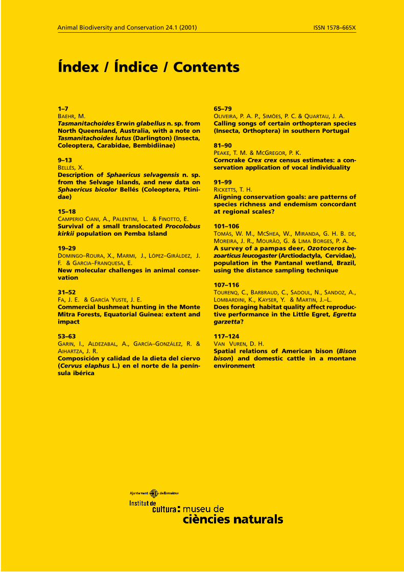
1–7Baehr, M. Tasmanitachoides Erwin glabellus n. sp. from North Queensland, Australia, with a note on Tasmanitachoides lutus (Darlington) (Insecta, Coleoptera, Carabidae, Bembi diinae)
9–13Bellés, X. Description of Sphaericus selvagensis n. sp. from the Selvage Islands, and new data on Sphaericus bicolor Bellés (Coleoptera, Ptini-dae)
15–18CaMperio Ciani, a., palentini, l. & Finotto, e. Survival of a small translocated Procolobus kirkii population on Pemba Island
19–29DoMingo–roura, X., MarMi, J., lópez–girálDez, J. F. & garCia–Franquesa, e. New molecular challenges in animal conser-vation
31–52Fa, J. e. & garCía Yuste, J. e. Commercial bushmeat hunting in the Monte Mitra Forests, Equatorial Guinea: extent and impact
53–63garin, i., alDezaBal, a., garCía–gonzález, r. & aihartza, J. r. Composición y calidad de la dieta del ciervo (Cervus elaphus L.) en el norte de la penín-sula ibérica
65–79oliveira, p. a. p., siMões, p. C. & quartau, J. a.Calling songs of certain orthopteran species (Insecta, Orthoptera) in southern Portugal
81–90peake, t. M. & MCgregor, p. k. Corncrake Crex crex census estimates: a con-servation application of vocal indiv iduality
91–99riCketts, t. h. Aligning conservation goals: are patterns of species richness and endemism concor dant at regional scales?
101–106toMás, W. M., MCshea, W., MiranDa, g. h. B. De, Moreira, J. r., Mourão, g. & liMa Borges, p. a. A survey of a pampas deer, Ozotoceros be-zoarticus leucogaster (Arctiodactyla, Cervidae), population in the Pantanal wetland, Brazil, using the distance sampling technique
107–116tourenq, C., BarBrauD, C., saDoul, n., sanDoz, a., loMBarDini, k., kaYser, Y. & Martin, J.–l. Does foraging habitat quality affect reproduc-tive performance in the Little Egret, Egretta garzetta?
117–124van vuren, D. h. Spatial relations of American bison (Bison bison) and domestic cattle in a montane environment
Índex / Índice / Contents
Animal Biodiversity and Conservation 24.1 (2001) ISSN 1578–665X