Anisotropy estimation based on the grey level co ... · For a simple 2D image and a standard offset of ... we often refer to seismic anisotropy, ... for five different stratigraphic

© 2016 EAGE www.firstbreak.org 83

special topicfirst break volume 34, March 2016

Modelling/Interpretation

1 Geo5 GmbH, Leoben, Austria.2 MOL, Budapest, Hungary.* Corresponding author, E-mail: [email protected]

The sample points being compared are aligned in different directions. For a simple 2D image and a standard offset of one pixel, the number of neighbouring pixels is eight and the number of possible directions is four (Eichkitz et al., 2015a, 2015b). Eichkitz et al. (2013) described how GLCM calcula-tions could be expanded to three dimensions. For 3D data and a sample offset of one, there are 26 neighbouring sam-ples that are aligned in 13 different directions. Increasing the sample offset increases the number of neighbouring samples. A sample offset of two means that the direct neighbouring samples are skipped and comparisons are made with the next sample points. Then, a centre sample point has 98 second–neighbouring samples and these are aligned in 49 directions (Figure 1).

For GLCM calculations, a small analysis window is extracted and within this all possible sample combinations

Anisotropy estimation based on the grey level co-occurrence matrix (GLCM)

Christoph Georg Eichkitz1*, Johannes Amtmann1, Marcellus Gregor Schreilechner1 and Sarah Schneider2 focus on the application of textural attributes to estimate volumetric anisotropy based on the grey level co-occurrence matrix (GLCM).

A nisotropy refers to directional properties. In geophys-ics, we often refer to seismic anisotropy, the depend-ence of velocity on direction or upon angle (e.g., Crampin 1981, 1985; Lynn and Thomsen, 1990;

Willis et al., 1986, Martin and Davis, 1987; Thomsen, 1986; Alkhalifah and Tsvankin, 1995). Variation in seismic veloc-ity with direction may reflect lateral changes in facies, the presence of faults or fractures, or differences in pore fillings, among many factors that may influence velocity. In principal, seismic data can be used to estimate volumetric azimuthal anisotropy (Simon, 2005). In this work we focus on the application of textural attributes to estimate volumetric ani-sotropy. The grey level co-occurrence matrix (GLCM), initially described by Haralick et al. (1973) as a tool for image clas-sification, is a measure of how often different combinations of pixel brightness values occur in an image. This method has widely been used for classification of satellite images (Franklin, et al., 2001; Tsai, et al., 2007), sea-ice images (Soh and Tsatsoulis, 1999; Maillard et al., 2005), and magnetic resonance and computed tomography images (Kovalev et al., 2001; Zizzari et al., 2011). This methodology can also be applied to seismic data to describe facies, reservoir properties, and fractures (Vinther et al., 1996; Gao, 1999, 2003, 2007, 2008a, 2008b, 2009, 2011; West et al., 2002; Chopra and Alexeev, 2005, 2006a, 2006b; Yenugu et al., 2010; de Matos et al., 2011; Eichkitz and Amtmann et al., 2012b, 2013, 2014, Eichkitz and de Groot et al., 2014; Eichkitz et al., 2015a, 2015b). GLCM–based attributes can be calculated in different directions, yielding an array of radial responses. By comparing these different results it is possible to determine anisotropy in the seismic data. Here, directional GLCM–based attributes are used for the description of channel structures and for the interpretation of fractured reservoirs.

Workflow for anisotropy detectionThe GLCM methodology belongs to the group of second–order texture classification methods in which the relation-ships between two sample points are measured. Usually, the sample points are neighbours, but the offset can be larger.

Figure 1 For an offset of one, each sample point has 26 neighbouring cells (a). These neighbouring cells are aligned in 13 directions. For an offset of two, the number of neighbouring pixels increases to 98, aligned in 49 directions (b).

special topic


www.firstbreak.org © 2016 EAGE84

first break volume 34, March 2016

workflow consists of three main steps (Figure 2). First, parameters for the calculations must be defined, including the number of grey levels, the vertical and horizontal size of the analysis window, and the sample offset. Depending on the sample offset, GLCM calculations will be done in 13 directions (offset = 1) or 49 directions (offset = 2). Next, in step 2 of the workflow, one GLCM based attribute is calculated in all directions, producing either 13 or 49 attribute cubes. In the final step, these 13 or 49 attribute cubes are compared. For each sample point, the minimum and maximum values of the attribute cubes are determined and the directions in which these values occur are stored.

The maximum and minimum values can be used as indi-cators of anisotropic areas. Dividing the maximum values by the minimum yields a new attribute, the anisotropy fac-tor. The anisotropy factor is an expression of the anisotropy present at each sample point. In the very rare circumstance that both the maximum and minimum are the same, the anisotropy factor equals 1 and area is isotropic. The range of the anisotropy factor depends on the scale of the GLCM attribute used. For GLCM energy, the anisotropy factor ranges between 1 and 10. Attributes such as GLCM vari-ance will yield a smaller range in anisotropy factor.

As the value of 1 for the anisotropy factor can rarely be found, this may lead to an overestimation of the ani-sotropy in some areas. To avoid this, the final results can be conditioned by applying a threshold or cut-off value. All areas where the anisotropy factor is below a certain threshold value are set to undefined, while other other areas are assigned their minimum and maximum values and the corresponding directions of the minimum and maximum values.

For a definitive description of seismic anisotropy, this procedure should be repeated using several GLCM–based attributes and the results combined. It is then possible to describe areas that have greater directional variability, which may be an indicator of changes in lithology, pore filling, or density of fractures.

Application of the workflowThis workflow was tested for two different applications. The first is a suspected channel system in Miocene sediments of the Vienna Basin in Austria. The objective of the study was to describe the channel system using GLCM–based attributes and obtain information about the internal structure of the channels. The second case study is fracture detection within the Carboniferous (Pennsylvanian) Tensleep Formation at Teapot Dome in Wyoming, USA. In this study, the aim was to map fracture intensities and orientations in terms of fracture dip and azimuth.

A channel system was identified at depth of approxi-mately 1000 ms by conventional coherence attribute analysis (Eichkitz et al., 2012a) in a seismic survey of the

are written into a symmetric matrix having the same size as the number of grey levels used. GLCM-based attributes are based on a normalized version of this matrix, found by dividing all matrix entries by the total number of co-occurrences. This produces a matrix of proportions that may be regarded as a kind of probability matrix. A number of attributes can be calculated based on this probability matrix (Haralick et al., 1973) and assigned to the central point of the analysis window. To determine GLCM–based attributes for the entire dataset, this procedure is repeated within a moving window.

Calculations performed in different directions will give slightly different results. Based on this observation, a workflow can be developed that automatically detects such directional differences for an entire seismic cube. The

Figure 2 The workflow consists of three steps. In the first step, the number of grey levels, size of the analysis window and offset are defined. The second step is calculation of GLCM attributes in all previously defined directions. For each sample point, maximum and minimum attribute values and the direction they occur in are determined. The third step is plotting results. Depending on the GLCM attribute, the direction of maximum or minimum attribute values defines the direction of anisotropy. The ratio of maximum to minimum value defines the anisotropy factor.

special topic




Figure 4 (Upper) Amplitude and coherence for time-slice shown in Figure 3. (Lower) Anisotropy directions and anisotropy factor calculated for four GLCM–based attributes. Best results are achieved with GLCM–based energy and homogeneity, which also show higher differences between maximum and minimum values (see scale on images).

Figure 3 Calculation of GLCM-based energy in 13 directions. In the time-slices small variations are observable. The channel structure is especially vis-ible in calculations done with 0° dip. Dotted lines indicate channel system interpreted on coherence cube (Eichkitz, et al., 2012a).

special topic




Figure 5 Anisotropy factor based on GLCM energy for five different stratigraphic intervals at Teapot Dome. In the Opeche Shale there are only a few areas with higher anisotropy factor. There are more areas with a high anisotropy factor In Tensleep A Sandstone, Tensleep B Dolomite, Tensleep B Sandstone and Tensleep C1 Dolomite. The anisotropy factor can be correlated with frac-ture intensities in these areas.

Figure 6 Azimuth direction of maximum values of GLCM-based energy. In combination with the information from Figure 5, these directions can directly be used as indicators of fracture directions.

special topic




have been published (e.g. Gilbertson, 2006; Zhang, 2005; Wilson et al., 2013b, 2015, Schwartz, 2006). The use of seismic attributes to describe Tensleep fractures has been investigated by Ouenes et al. (2010), Gao (2013), Wilson et al., (2012, 2013a, 2013b, 2015), Di and Gao (2014), and Thachaparambil (2015).

In this study, post-stack seismic attributes including coherence, curvature, and spectral decomposition (Schneider, et al., 2015) were used in addition to GCLM-based attributes. The parameters for the GLCM–based attribute calculations were similar to those used in the channel study with 64 grey levels and an analysis window of 3 x 3 x 15. Calculations were made in 13 directions and the results compared with each other. The anisotropy factor was especially important because it is an indicator of fracture intensity. In this case study, the anisotropy factor should be highest in the Tensleep B stratigraphic zone and lower in the Tensleep C and in the Opeche Shale where fracturing is known to be less intense. This is clearly apparent in Figure 5, which shows maps of the anisotropy factor for the Opeche Shale, Tensleep A Sandstone, Tensleep B Dolomite, Tensleep B Sandstone, and Tensleep C1.

In addition to the anisotropy factor, the workflow pro-duces directions of anisotropy that can be correlated with the strike and dip of fractures. Depending on the GLCM–based attribute, the strike direction is either perpendicular to the direction of maximum value or is parallel. For GLCM–based energy, the strike direction is perpendicular to the direction of maximum value, so energy–based azi-muths and dips must be shifted to obtain fracture dip and azimuth. In Figure 6, corrected fracture azimuths based on GLCM energy are shown for the Opeche Shale, Tensleep A

Vienna Basin. The channel deposits have a width of approximately 130-300 m, an average thickness of 70 ms, and occur in strata that most probably are of Sarmatian or Pannonian age (Middle to Upper Miocene). For the study, the number of grey levels was set to 64, and the analysis window was three samples in inline and crossline directions and 11 samples in the vertical direction. Using these parameters, GLCM–based attributes were calculated in 13 directions. Figure 3 shows results using GLCM–based energy. Most areas outside the channel have very low energy values. Inside the channel, there are small variations in energy depending on direction. Attributes calculated with a dip of zero have higher energy readings than others, sug-gesting that greater variation in seismic facies is expected in horizontal directions. A visual comparison of results for 0° dip and different azimuths is difficult, but by applying the anisotropy factor procedure to the different attribute sets and setting threshold values different facies within the channel are revealed (Figure 4). In this example, ener-gy gives the best results and also exhibits the highest anisotropy factor.

The objective of the second case study was to character-ize a fractured reservoir. Teapot Dome, located in central Wyoming, is the extension of a large structural complex with the Salt Creek anticline to the north and the Sage Spring Creek and Cole Creek oil fields to the south (Doelger et al., 1993; Gay, 1999; Cooper et al., 2001). Stratigraphic units of interest are the Pennsylvanian Tensleep Formation and Opeche Shale. The Tensleep Formation serves as a reservoir interval in several Rocky Mountain oil fields and consists predominantly of naturally fractured sandstone. Numerous studies of fracturing in the Tensleep Formation

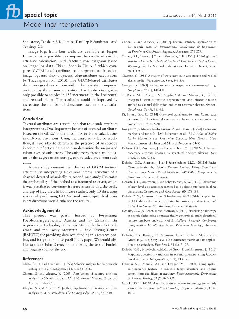
Figure 7 Rose diagrams for well 48-X-48. Comparison of fracture strike and dip of image log data (orange) with maximum azimuth and dip of GCLM-based attributes energy (blue), entropy (green), homogeneity (rose), contrast (turquoise), variance (violet), and dissimilarity (yellow). The last column shows the results of Thachaparambil (2015), where spectral edge attribute calculations were converted into discrete objects called SDPs, to compare their azimuth and dip with image log data.

special topic




Chopra S. and Alexeev, V. [2006b] Texture attribute application to

3D seismic data. 6th International Conference & Exposition

on Petroleum Geophysics, Expanded Abstracts, 874-879.

Cooper, S.P., Lorenz, J.C. and Goodwin, L.B. [2001] Lithologic and

Structural Controls on Natural Fracture Characteristics Teapot Dome,

Wyoming. Sandia National Laboratories, Technical Report, Sand,

2001–1786.

Crampin, S. [1981] A review of wave motion in anisotropic and racked

elastic-media. Wave Motion, 3 (4), 343-391.

Crampin, S. [1985] Evaluation of anisotropy by shear-wave splitting.

Geophysics, 50 (1), 142-152.

de Matos, M.C., Yenugu, M., Angelo, S.M. and Marfurt, K.J. [2011]

Integrated seismic texture segmentation and cluster analysis

applied to channel delineation and chart reservoir characterization.

Geophysics, 76 (5), P11-P21.

Di, H. and Gao, D. [2014] Gray-level transformation and Canny edge

detection for 3D seismic discontinuity enhancement. Computers &

Geosciences, 72, 192–200.

Doelger, M.J., Mullen, D.M., Barlow, D. and Haun, I. [1993] Nearshore

marine sandstone. In: J.M. Robertson et al. (Eds.) Atlas of Major

Rocky Mountain gas Reservoirs: Socorro, New Mexico, New

Mexico Bureau of Mines and Mineral Resources, 54-55.

Eichkitz, C.G., Amtmann, J. and Schreilechner, M.G. [2012a] Enhanced

coherence attribute imaging by structural oriented filtering. First

Break, 30 (3), 75-81.

Eichkitz, C.G., Amtmann, J. and Schreilechner, M.G. [2012b] Facies

Characterization by Seismic Texture Analysis Using Grey Level

Co-occurrence Matrix Based Attributes. 74th EAGE Conference &

Exhibition, Extended Abstracts.

Eichkitz, C.G., Amtmann, J. and Schreilechner, M.G. [2013] Calculation

of grey level co-occurrence matrix-based seismic attributes in three

dimensions. Computers and Geosciences, 60, 176-183.

Eichkitz, C.G., Amtmann, J. and Schreilechner, M.G. [2014a] Application

of GLCM-based seismic attributes for anisotropy detection. 76th

EAGE Conference & Exhibition, Extended Abstracts.

Eichkitz, C.G., de Groot, P. and Brouwer, F. [2014] Visualizing anisotropy

in seismic facies using stratigraphically constrained, multi-directional

texture attribute analysis. AAPG Hedberg Research Conference

‘Interpretation Visualization in the Petroleum Industry’, Houston,

USA.

Eichkitz, C.G., Davis, J. C., Amtmann, J., Schreilechner, M.G. and de

Groot, P. [2015a] Grey Level Co-Occurrence matrix and its applica-

tion to seismic data. First Break, 33 (3), 71-77.

Eichkitz, C.G., Schreilechner, M.G., de Groot, P. and Amtmann, J. [2015]

Mapping directional variations in seismic character using GLCM-

based attributes. Interpretation, 3 (1), T13-T23.

Franklin, S.E., Maudie, A.J. and Lavigne, M.B. [2001] Using spatial

co-occurrence texture to increase forest structure and species

composition classification accuracy. Photogrammetric Engineering

& Remote Sensing, 67 (7), 849-855.

Gao, D. [1999] 3-D VCM seismic textures: A new technology to quantify

seismic interpretation. 69th SEG meeting, Expanded Abstracts, 1037-

1039.

Sandstone, Tensleep B Dolomite, Tensleep B Sandstone, and Tensleep C1.

Image logs from four wells are available at Teapot Dome, so it is possible to compare the results of seismic attribute calculations with fracture rose diagrams based on image log data. This is done in Figure 7 which com-pares GCLM-based attributes to interpretations based on image logs and also to spectral edge attribute calculations by Thachaparambil (2015). The GLCM–based attributes show very good correlation within the limitations imposed on them by the seismic resolution. For 13 directions, it is only possible to resolve in 45° increments in the horizontal and vertical planes. The resolution could be improved by increasing the number of directions used in the calcula-tions.

ConclusionTextural attributes are a useful addition to seismic attribute interpretation. One important benefit of textural attributes based on the GLCM is the possibility to doing calculations in different directions. Using the anisotropy factor work-flow, it is possible to determine the presence of anisotropy in seismic reflection data and also determine the major and minor axes of anisotropy. The anisotropy factor, an indica-tor of the degree of anisotropy, can be calculated from such data.

A case study demonstrates the use of GLCM textural attributes in interpreting facies and internal structure of a channel detected seismically. A second case study illustrates the applicability of the method to a fractured reservoir, where it was possible to determine fracture intensity and the strike and dip of fractures. In both case studies, only 13 directions were used; performing GLCM-based anisotropy calculations in 49 directions would enhance the results.

AcknowledgementsThis project was partly funded by Forschungs Foerderungsgesellschaft Austria and by Zentrum für Angewandte Technologien Leoben. We would like to thank OMV and the Rocky Mountain Oilfield Testing Centre (RMOTC) for providing data sets, funding this research pro-ject, and for permission to publish this paper. We would also like to thank John Davies for improving the use of English and organization of the text.

ReferencesAlkhalifah, T. and Tsvankin, I. [1995] Velocity analysis for transversely

isotropic media. Geophysics, 60 (5), 1550-1566.

Chopra, S. and Alexeev, V. [2005] Application of texture attribute

analysis to 3D seismic data. 75th SEG Annual Meeting, Expanded

Abstracts, 767-770.

Chopra, S. and Alexeev, V. [2006a] Application of texture attribute

analysis to 3D seismic data. The Leading Edge, 25 (8), 934-940.

special topic




Simon, Y.S. [2005] Stress and fracture characterization in a shale reser-

voir, north Texas, using correlation between new seismic attributes

and well data. M.S. thesis, University of Houston, Houston,

Texas.

Soh, L.-K. and Tsatsoulis, C. [1999] Texture analysis of SAR sea ice

imagery using gray level co-occurrence matrices. IEEE Transactions

on Geoscience and Remote Sensing, 37 (2), 780-795.

Thachaparambil, M.V. [2015] Discrete 3D fracture network extraction

and characterization from 3D seismic data – A case study at Teapot

Dome. Interpretation, 3 (3), ST29-ST41.

Thomsen, L. [1986] Weak elastic anisotropy. Geophysics, 51 (10),

1654-1966.

Tsai, F., Chang, C.-T., Rau, J.-Y., Lin, T.-H. and Liu, G.-R. [2007] 3D

computation of grey level co-occurrence in hyperspectral image

cubes. LNCS 4679, 429-440.

Vinther, R., Mosegaar, K., Kierkegaard, K., Abatzi, I., Andersen,

C., Vejbaek, O.V., If, F. and Nielsen, P.H. [1996] Seismic tex-

ture classification: A computer-aided approach to stratigraphic

analysis. 65th SEG Annual Meeting, Expanded Abstracts, 153-

155.

West, B.P., May, S.R., Eastwood, J.E. and Rossen, C. [2002] Interactive

seismic facies classification using textural attributes and neural

networks. The Leading Edge, 21 (10), 1042-1049.

Willis, H., Rethford, G., and Bielanski, E. [1986] Azimuthal anisotropy:

Occurrence and effect on shear wave data quality. 56th Annual

International Meeting, Expanded Abstracts.

Wilson, T. H., Smith, V., Brown, A. L., and Gao, D. [2012] Modeling

discrete fracture networks in the Tensleep sandstone: Teapot Dome,

Wyoming. AAPG Annual Convention and Exhibition, Search and

Discovery Article, #50658.

Wilson, T. H., Smith, V., and Brown, A. L. [2013a] Developing a strategy

for CO2 EOR in an unconventional reservoir using 3D seismic attrib-

ute workflows and fracture image logs. 82nd SEG Annual Meeting,

Expanded Abstracts, 2563-2567.

Wilson, T. H., Smith, V. and Brown, A. L. [2013b] Characterization of

Tensleep reservoir fracture systems using outcrop analog, fracture

image logs and 3D seismic. AAPG Rocky Mountain Section Meeting,

Search and Discovery Article #50877.

Wilson, T.H., Smith, V. and Brown, A. [2015] Developing a model discrete

fracture network, drilling, and enhanced oil recovery strategy in an

unconventional naturally fractured reservoir using integrated field,

image log, and three-dimensional seismic data. AAPG Bulletin, 99

(4), 735-762.

Yenugu, M., Marfurt, K.J. and Matson, S. [2010] Seismic texture analysis

for reservoir prediction and characterization. The Leading Edge, 29

(9), 1116-11.

Zhang, Q. [2005] Stratigraphy and sedimentology of the Tensleep sand-

stone at the Teapot Dome and in outcrops. Wyoming. M.S. thesis,

Colorado School of Mines.

Zizzari, A., Seiffert, U., Michaelis, B., Gademann, G. and Swiderski,

S. [2001] Detection of tumor in digital images of the brain. Proc.

of the IASTED international conference Signal Processing, Pattern

Recognition & Applications, 132-137.

Gao, D. [2003] Volume texture extraction for 3D seismic visualization

and interpretation. Geophysics, 68 (4), 1294-1302.

Gao, D. [2007] Application of three-dimensional seismic texture analysis

with special reference to deep-marine facies discrimination and

interpretation: Offshore Angola, West Africa. AAPG Bulletin, 91

(12), 1665-1683.

Gao, D. [2008a] Adaptive seismic texture model regression for subsurface

characterization. Oil & Gas Review, 6 (11), 83-86.

Gao, D. [2008b] Application of seismic texture model regression to

seismic facies characterization and interpretation. The Leading Edge,

27 (3), 394-397.

Gao, D. [2009] 3D seismic volume visualization and interpretation: An

integrated workflow with case studies. Geophysics, 74 (1), W1-

W24.

Gao, D. [2011] Latest developments in seismic texture analysis for

subsurface structure, facies, and reservoir characterization: A review.

Geophysics, 76 (2), W1-W13.

Gao, D. [2013] Integrating 3D seismic curvature and curvature gradient

attributes for fracture characterization: Methodologies and interpre-

tational implications. Geophysics, 78 (2), O21–O31.

Gay, S.P. Jr. [1999] An explanation for ‘4-way closure’ of thrustfold

structures in the Rocky Mountains, and implications for similar

structures elsewhere. The Mountain Geologist, 36 (4), 235-244.

Gilbertson, N.J. [2006] 3D geologic modeling and fracture interpretation

of the Tensleep Sandstone, Alcova anticline, Wyoming. M.S. thesis,

Colorado School of Mines, Golden, Colorado.

Haralick, R.M., Shanmugam, K. and Dinstein, I. [1973] Textural features

for image classification. IEEE Transactions on systems, man, and

cybernetics, 3 (6), 610-621.

Kovalev, V.A., Kruggel, F., Gertz, H.-J. and von Cramon, D.Y. [2001]

Three-dimensional texture analysis of MRI brain datasets. IEEE

Transactions on medical imaging, 20 (5), 424-433.

Lynn, H.B. and Thomsen, L.A. [1990] Reflection shear-wave data col-

lected near the principal axes of azimuthal anisotropy. Geophysics,

55 (2), 147-156.

Maillard, P., Clausi, D.A. and Deng, H. [2005] Operational map-

guided classification of SAR sea ice imagery. IEEE Transaction on

Geoscience and Remote Sensing, 43 (12), 2940-2951.

Martin, M.A. and Davis, T.L. [1987] Shear-wave birefringence: A new

tool for evaluating fractured reservoirs. The Leading Edge, 6 (10),

22-28.

Ouenes, A., Anderson, T., Klepacki, D., Bachir, A., Boukhelf, D.,

Araktingi, U., Holmes, M., Black, B. and Stamp, V. [2010] Integrated

characterization and simulation of the fractured Tensleep Reservoir

at Teapot Dome for CO2 injection design. SPE Western Regional

Meeting, SPE 132404.

Schneider, S., Eichkitz, C.G. and Schreilechner, M.G. [2015] Interpretation

and modeling of fractured zones using seismic attributes and image

log data – Teapot Dome, Wyoming. 77th EAGE Conference &

Exhibition, Madrid.

Schwartz, B. [2006] Fracture pattern characterization of the Tensleep

Formation, Teapot Dome, Wyoming. M.S. thesis, West Virginia

University, Morgantown, West Virginia.

Documents

Anisotropy estimation based on the grey level co ... · For a simple 2D image and a standard offset of ... we often refer to seismic anisotropy, ... for five different stratigraphic