Ann. Inst. Statist. Math. - 統計数理研究所 · ann. inst. statist. math. vol. 47, no. 2, 351 369 (1995) stochastic regression model with heteroscedastic disturbance* der-shin

Ann. Inst. Statist. Math. Vol. 47, No. 2, 351 369 (1995)

STOCHASTIC REGRESSION MODEL WITH HETEROSCEDASTIC DISTURBANCE*

DER-SHIN CHANG AND GUAN-CHYUN LIN

Institute of Statistics, National Tsing Hua University, Hsinchu, Taiwan 30043, R.O.C.

(Received February 28, 1994; revised September 12, 1994)

A b s t r a c t . This paper discusses some properties of stochastic regression model with continuous form of heteroscedastic disturbance. The strong consis- . tency and asymptotic normality of a generalized weighted least squares estimate will be investigated under certain conditions on the stochastic regressors and errors. More, the linear hypothesis testing problem also be discussed and an example to be demonstrated to reestablish the results of Cheng and Chang (1990, Tech. Report, National Tsing Hua University).

Key words and phrases: Stochastic regressors, generalized weighted least squares, strong consistency, asymptotic normality, linear hypothesis, martin- gales, heteroscedastic disturbance.

1. Introduction

Consider the multiple regression model

(1.1) Yn =/31Xnl ÷ fl2Xn2 + " " +/3pXnp + Cn, n = 1 , 2 , . . .

where e~'s are unobservable random errors, /~1,-.. ,/~p are unknown parameters , and Yn is the observed response corresponding to the design levels xnl , x ~ 2 , . . . , Xnp. Let x n = ( X n l , . . . , X n p ) T, X n = (Xij)l<i<_n,l<_j<p , E n = (61 , . . . , 5n ) T and Y~ = ( Y l , . . . , y , ) T . The regression model (1.1) can be wri t ten as Y~ = X~/3 + En where ¢~ = (¢~l"' '/~p)T and the ordinary least squares es t imate of fl based on the x l , Y l , . . . , Xn, y~ is bn = (b~l" ' " b~p) T = ( X [ X n ) - - I x [ y ~ , assuming X ~ X n nonsingular. Suppose tha t {e~} is a mart ingale difference sequence with respect to an increasing sequence of or-fields {.7-} i.e. en is iOn-measurable and E(en I JC,_l) = 0 for every n, more, assume tha t the design vector Xn at stage n depends on the previous observations Xl, Y l , . . . , xn-1 , y~ - l ; i.e. xn is 5~ 1-measurable. In the case of homoscedast ic disturbance, i.e. E(e 2 ] 5 ~ - 1 ) = cr 2 for every n, the strong consistency and asymptot ic normal i ty of the least squares es t imate b~ has

* Supported by the National Science Council Grant No. 810208M763 at National Tsing Hua University.

351

352 DER-SHIN CHANG AND GUAN-CHYUN LIN

been established by Lai and Wei (1982), similar properties were also studied by Cheng and Chang (1990) under some regular conditions for the special case of linear heteroscedasticity.

In this paper we shall study the properties of a more general form, the continuous heterosedastic disturbance, which will generalize those of the above two cases. In Section 3 we try to establish the strong consistency and asymptotic normality of a generalized weighted least squares estimate under certain conditions on the stochastic regressors and errors. In Section 4 we will discuss the linear hypothesis testing problem in this model. In Section 5 we reestablish the results of Cheng and Chang (1990) from Corollary 5.1, Theorems 3.2, 3.4 and 4.1.

2. Some reviews

In this sections we review some important results in Lai and Wei (1982). In model (1.1), they assume:

(2.1) sup ]~{ [e n [ e~ [ .-~"n--1} < OO n

and

(2.2) l i ra E{6~ I 5r~_1} = ~ 2

a.s. for some (~ > 2

a.s. for some positive constant a2.

A special case of (2.2) is E(e~ ] 5~n-1) = (7 2 for every n. Let Ama×(A), Amin(A), Am~x(n) and Amin(n), respectly, denotes the maximum and minimum eigenvalue of matrix A and x T x n . They established the strong consistency of bn =

T --1 T (X~ XN) X~ Y~ under the assumption that /~min(n) tend to infinity faster than log/~max(n) in the following result.

Suppose that in the regression model (1.1), {en} satisfies

/~min(n) ----+ OO a.8.,

log -~max(n) = O(/~min(n)) a.8.

TH EO REM 2.1.

(2.1) and

then bn -+/3 a.s.

This result follows from the key

LEMMA 2.1. Let {en} be a martingale difference sequence with respect to an increasing sequence of a-fields {5cn} such that supn E(le~l ~ I 9Cn-1} < ec a.s. for some a > 2. Let Xnl , . . . , Xnp be .~_l-measurable random variable for every n. Define N = inf{n : x T x n is nonsingular} and Qn ~--- E T n X ~ ( X T X ~ ) - I x T E n , assume N < ec a.s. Then for n > N and on {l im~_~ Ama×(n) = ee} we have

Q n = O ( l o g ~ m a ~ ( n ) ) a.8.

S T O C H A S T I C R E G R E S S I O N M O D E L 353

3. Estimation problem

In this section we will discuss the same estimation problem under that E(e~ I 9v~-1) = g(Zn, 0), where Zn is observable and 5On_l-measurable, Zn and 0 belong to the k-dimensional Euclidean space, g is a real-valued known function of z~ and 0 (0 unknown parameter vector). Let s~ . . . . (X~l/S~. . . x~p/sn) T and e~ = e~/sn for every n, then we can rewrite model (1.1) a s

(3.1) T r l~=wn/3+e~ , n = 1 ,2 , . . . .

Note that E * (e~ I 9c~ 1) = 1 for every n and the weighted least squares estimate of/3, denoted by l)~, in model (1.1) is just the ordinary least squares estimate of

in model (3.1). Since 0 is unknown, we substitute the 0n described below into ¢)n, and get a generalized weighted squares estimates 2)* of/3. In order to prove our main results, we need following Lemmas.

LEMMA 3.1. (Jennrich (1969)) Let f be a real valued function on @ x Y where (9 be a compact subset of a Euclidean space and Y is a measurable space. For each 0 in O, let f(O, y) be a measurable function of y and a continuous function of 0 for each y in Y . Then there exists a measurable function 0 from Y into 0 such that for all y in Y

f(O(y), y) = inf f(O, y). O c O

LEMMA 3.2. (Lai and Wei (1982), (4.15)) Suppose that {en} is a martingale difference sequence with respect to an increasing sequence of a-fields {Sen} such that (2.1) holds, then

n n

Z 4 = E E(41fi-1)+ o(n) i : 1 i : 1

a . s .

LEMMA 3.3. Let A, 0 be subsets of k-dimensional Euclidean space, more, assume that A is a compact set. I f f ( z , p) is real valued function which is continuous on A x 6), then SUpz~z x f ( z , p) and inf~e/, f ( z , p) are continuous functions ofp.

PROOF. See Appendix.

Now since En Yn Xnbn (In T -1 T . . . . Xn(Xn X~) X~)En where we denote /)~ = [el, e2 , . . . , en]T. Define the least squares estimate 0~ of 0 to be the value of p that minimizing Qn (p) = }-~.tn 1 [~2 _ g(zt, p)]2/n, that is Q~ (0~) = infpce Qn (p).

THEOREM 3.1. Suppose that in the regression model (1.1), {~n) is a martingale difference sequence with respect to an increasing sequence of a-fields {)cn}


s u c h t h a t ( 2 . 1 ) h o l d s a n d E(e~ I " ) r ' n -1 ) = ~ ( Z n , O) f o r e v e r y ~ , w h e r e g i s a peal

valued known function of z~ and unknown parameter vector O. We assume (i) the parameter vector 0 is contained in a bounded open sphere S where the

closure of S is denoted by O, (ii) sup~ [[z~[lk < oe a.s., where [[. [[k denotes the k-dimensional Euclidean

n o r m ,

(iii) g is continuous function on R k × 0 and g(z~, p) > 0Vp ¢ {0, 01, . . . , 0~ , . . .} a .s . ,

(iv) the quantity n

lim -1 E ( g ( z t , O) _ g(zt ,p)) 2 n---~ oo n

t = l

has a unique minimum at p = 0 a.s., (v) lOg am~x (n) /n -~ 0 a.s.

Then we have the least squares estimate On ~ 0 a.s.

PROOF. (a) Note first tha t the existence and measurabil i ty of the least squares est imate of 0 would be followed from Lemma 3.1. Next let ¢,~ = {w : SUpnllZn(W)llk <_ m} and Am = {z E R k : Ilzllk _< m}, then we have P ( U ~ = I ¢ ~ ) = 1 and ~ ~ ZX~ for an n on the set ¢~.

Since g is a continuous function on A,~ x (9 and A,~ x O is compact, there exists L2 such tha t g(zn, p) < L2 < c~Vn, p c 0 on the set ¢,~ for any m, thus we can assume without loss of generality in subsequence that supn IIz~(w)Ilk < m a.s.

For every Pn E (9, let An = d i a g ( ~ , . . . , v/g(zn, pn)). Then we have

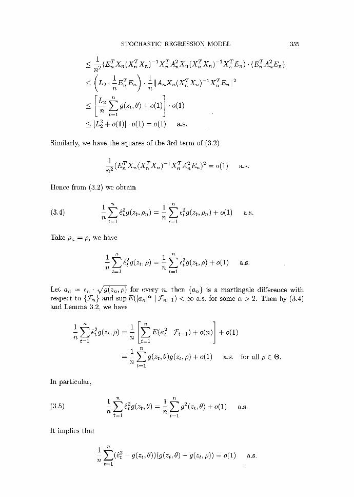
(3.2) _1 ~ 2 t g ( z t , p ~ ) = I (A~E~)T(A~E~ ) n

t : l 1 1 __ x ]JTT A 2 ]j " T 2 T 1 T - ~ , ~ - - E n & X ~ ( X ~ x , o x,~ E,~ n n

T T --1 T 2 1 E ~ X n ( X ~ X ~ ) X~AnE,~ n

1 T T - -1 T 2 T - 1 T +-E~X~(XnX~) XnA~X~(X~X~) X~En. n

Since the 4th t e rm of (3.2) equals to

(3.3) 1 2 T - 1 T 2

I I & X ~ ( X ~ X n ) - X X f Enll 2 <_ -Amax(An)l lX~(X~X~ ) X~E~[[ n

1 _< - L 2 ' O(logAmax(n)) (by Lemma 2.1)

n

= o(1) a.s.

Then by Cauchy-Schwarz inequality, Lemma 3.2 and (3.3), we have the square of the 2nd t e rm of (3.2)

1 T 2 T --1 T 2

S T O C H A S T I C R E G R E S S I O N M O D E L 3 5 5

1 T T - 1 T 2 T - 1 T T 2 <_~i(E~Xn(XnX,~) XnAnXn(X,~X~ ) X~E~).(E,~A~E,)

< (L2.1ETEn). 1 T - - I T ~HA~X~(XnXn) X,~Enll 2

_< Zg(~ ,0 ) + o(1) .o(1) L t = l '

_< [L 2 + o(1)], o(1) = o(1) a.s.

Similarly, we have the squares of the 3rd term of (3.2)

1 T T - 1 T 2 2 ~(E~Xn(XnXn ) X~A.En) = o(1) a . s .

Hence from (3.2) we obtain

(3.4) - 1 ~ ~2tg(zt,p~ ) = -l ~-~tg(zt, p~ ) + o ( 1 ) a.s. n ~

t = l t = l

Take p~ = p, we have

1~-~ l ~-~c2tg(zt, p)+ o(1) t = l t = l

a . s .

Let an -- cn" ~ p ) for every n, then {a~} is a martingale difference with respect to {Jrn} and supE([an[ ~ I $'~_1) < oe a.s. for some c~ > 2. Then by (3.4) and Lemma 3.2, we have

1E~2tg(z~,p) 1 E(a2t lJZt_l)+o(n) + o ( 1 ) Yt t = l 7t t = l

1 =-Eg(zt,O)g(zt,p)+o(1) a.s. for all p E O. 7~

t = l

In particular,

(3.5) 1 /

~ g ( z ~ , 0) = t = l t = l

a . s .

It implies that

n

! Z ( ~ _ g(z~, 0))(g(z. o) - g (z . p)) = o(1) n

t - - 1

a . s .

356 D E R - S H I N C H A N G A N D G U A N - C H Y U N LIN

(b) S i n c e

(3.6) n

e.(~.) = inf 1__ ~(~_g(~, ,p))~ pEO

t = l n

= ~nf ! ~_ , (~ -g (~ ,O)+ 9(z~,O)-g(~,p))~ pEO n

t = l

= inf Z(~-g(zt, O))2 pEO t = l

2 n + - ~ ( ~ , ~ - ~ ( ~ , o))(~(z~, o) - ~(~,, p))

n t = l

i n ]

rt t = l

=#,,(O)+o(~) as ,

by (a) and condition (iv). (c) Since 0 is compact, let {0nk} be any convergent subsequence of {0n} and

say 0~ --+ 0". By (3.4) and (3.5), we have

~2k

?~k t = l

1 na = - - ~ 4 g ( z , , 0 ~ ) + o ( 1 ) a.~.

Tbk $=1

- - nk 1 nk 1 ~e~[g(z~,O~)-g(z,,O*)]+--~g(zt, O)g(zt, O*)+o(1) a . s .

nk t = l nk t = l

By Lemmas 3.2 and 3.3, and ~n~ ~ 0*, we have

= sup z~EAm

± ~ ~[~(z,, ~n~)- ~2k t = l

1 na

T~k t = l

nk

n k zt E/Xm t = l

~g(z~, o) + o(1)

--* s u p , , . , , . , , , T _ , . ~ , , l , l g [ z , , v . ) _ g ( z t , v , ) l . ( ~ 2 . o ( l ) ) = o ( H a.s., zt~Am

a . s .


it implies that

Similarly,

Thus

1 n k ~ k

- - E ~g(zt , Onk) = __I E g ( z t , O)g(zt, O, ) + o ( 1 ) n k n k t = l t--1

n k

± ~ g(z,, 0)[g(z,, 0~) - g(z~, e*)] = o(1) ~ k t = l

n k

1_ E[&2 _ g(zt, O)][g(zt,O) - g(zt,Onk)] = o(1) ?~k t = l

and by the same arguments of (3.6), we have

a.s.

nk

1 F _ . ( g ( z . e ) _ g(z~,~ - - 0~k)) = o(1) nk t=l

Further,

nk

lim 1 E ( g ( z t , O, ) _ g ( z t , ~ n k ) ) 2 nk--*oc Tt k t = l

< lim sup (g(zt, O*) g(zt, ~k)) nk'--~oo Z t E A m

-- 0, by Lemma 3.3 and 0~k ~ 0".

Hence

nk

i Z ( g ( z ~ , O . ) _ g(z~,O))2 /~k t=l

a . s .

n k

= ! ~[(g(z~, e* ) - g(z~, ~n~))+ (g(z~, ~ ) - g(z~, e))] ~ n k t = l

nk ! _ ~ 2 = Z ( g ( z . O * ) g(z~, n~)) n k t = l

n k

2 ~(g(z~, onk) - g(z~, e))(g(z~, e*) - g(z~, ~)) + n--~ t=l

1 nk g(zt, O) ) 2 + - - > ( q ( z . u n ~ ) -

nk t = l h . . . . - - 4 - - - - -

1 nk ~ 2 . 2 L 2 . - - E Ig(zt'O*) - g(zt,Onk)l + o(1)

?~k t = l

_ < 4 L 2 - s u p Ig(zt,O*)-g(z~,O~)[+o(1)-~O as z,C/X~

a . s .

a.8.

n k ----+ (:x:) a . s .


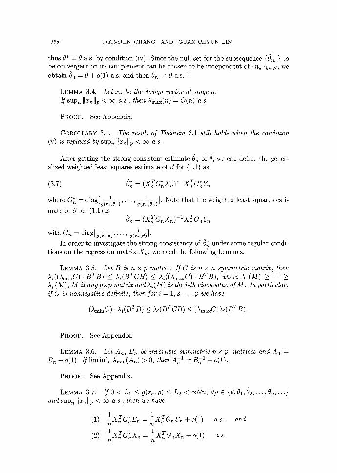
thus O* = 0 a.s. by condition (iv). Since the null set for the subsequenee {0~ k } to be convergent on its complement can be chosen to be independent of {nk}keN, we

obtain O, = 0 + o(1) a.s. and then ~}s --+ 0 a.s. []

LEMMA 3.4. Let xs be the design vector at stage n. I f SUPs Ilxsllp < ~ a.s., then/~max(n) = O(n) a.s.


COROLLARY 3.1. The result of Theorem 3.1 still holds when the condition (v) is replaced by supn IIx~llp < oo a.s.

After getting the strong consistent estimate O~ of 0, we can define the generalized weighted least squares estimate of/~ for (i.i) as

(3.7) /•n T * -- 1 T * -- (xs G~x~) x~ G~Y~

• 1 .. 1 ] Note tha t the weighted least squares esti- where G s = diag[9(~ ~ ) , . , g (~ ,~ ) .

mate of/3 for (1.1) is ) s T -- 1 T = (xn asxs) x~ asYs

with Gn = diag[~(zl,0), i ] "" , g(z,~,e) " In order to investigate the strong consistency of/3~* under some regular condi-

tions on the regression matr ix Xs, we need the following Lemmas.

LEMMA 3.5. Let B is n x p matrix. I f C is n x n symmetric matrix, then ~((~minC)" BTB) < ~(B~CB) < ~((~m~C)" BTB), ~here ~I(M) > - - > tp(M), M is a n y p x p matrix and I~(M) is the i-th eigenvalue of M. In particular, if C is nonnegative definite, then for i = 1, 2 , . . . ,p we have

( , ~ m i n C ) ' ) k i ( B T B ) ~ )h ( BT C B) <_ ( AmaxC)Ai( BT B).


LEMMA 3.6. Let As, Bs be invertible symmetric p x p matrices and An = Bs + o(1). I f liminfs/~min(An) > 0, then A~ 1 = B~ 1 + o(1).


LEMMA 3.7. IfO < L1 <<_g(zs, p) < L2 < ooVn, V p c {0 ,01 ,02 , . . . ,0n , . . . } and sup s HXnllp < 00 a.s., then we have

(1) lxr<E~ = ! x r G ~ E n + o(1) a.s. and n n 1 T • 1 (2) ~xs Gnxs ~x$anx~ + o(1) a.s.

STOCHASTIC REGRESSION MODEL

Furthermore, l iminfn Amin(n)/n > O, then

( 1 X T GnXn : X GnXn +o(1 ) a.s.

359


THEOREM 3.2. Suppose that in the regresswn model (1.1), {en} is a martingale difference sequence with respect to an increasing sequence of or-fields {3on} such that (2.1) holds and E(e~ I ~n-1) = g(zm 0), with g a known function and 0 unknown parameter vector. I f the regression matrix Xn and g(Zn, O) satisfy conditions (i), (ii), (iii), (iv) of Theorem 3.1 and the more extra conditions

(v) sup Ilxnll < a.s. and (vi) l iminfn)~min(n)/n > 0 a.s.

then fl~ ~ fl a.s.

PROOF. Let ¢,~, L2 as in the proof of Theorem 3.1. By Lemma 3.3 and 0n -~ 0, we have inft g(zt, On) ~ inft g(zt, O) a.s. Since inft g(zt, p) > 0Vp e {0, 01 , . . . , 0 m . . . } a.s. we take 0 < e < inft g(zt, 0). For this e, there exists N such that

inft g(zt, 0n) > inf g(zt, O) - e Vn > N,

take L1 = min{inft g(zt, 01), inft g(zt, 02) , . . . , inft g(zt, ON), inft 9(zt, 0) -- e}, then 0 < L1 ~ g(Zn, p) ~ L2 < (:X)V?~ and Vp c {0, 01 ,02 , . . . , 0n , . . . } a.s. By Lemma 3.4, condition (vi) and Lemma 3.5, we have

)~min(n) ~ (X:) a.s.,

log/~max (n) n lim sup - n ~min (n) X--n

1 log ~max (n) < - liminf~(/~min(n)/n) n

Ll (Z:VnXn) <

and

- o ( 1 ) a.s.,

<_ L2)~i(Xf GnXn)Vi -- 1, 2 , . . . ,p

/~min(XTn G n X n ) --+ oo,

a.s.,

log Am~x(X~ GnX~) = o ( . ~ m i n ( X T a n X n ) ) a.s.

Let en as in (3.1), since supn E(lenl ~ I 5on_l) < oo a.s. and by Theorem 2.1 we have

/~n T --1 T = ( X n G n x n ) X n G n Y n = f l + o ( 1 ) a.s.

Now we rewrite

~* fl T * --1 T * T * --1 T * -- : ( X n G n X n ) X n G n Y n - f l = ( X n G n X n ) X n G n E n .


Since the elements of Gn are bounded a.s., by condition (V), Lemma 3.7 and (2.9) of Lai and Wei (1982), we have

^* ¼X U.tn [ l and

+ o ( 1 ) = (~n - /3 )+o(1 ) =o(1)

/~ =/3 ÷ o(1) a.s.

Thus we conclude the result ~ --+ /3 a.s.

Before proving the asymptotic normality of/~*, we would like first to give a weaker form of asymptotic normality of b~ than that of Lai and Wei (1982), and try to study the asymptotic normality of ¢)~ to a more general result. Denote 2+

d and -~, respectively, the convergence in probability and in distribution.

THEOREM 3.3. (Chang and Chang (1990)) Suppose that in the regression model (1.1), {an} is a martingale difference sequence with respect to an increasing sequence of a-fields {~:n} such that (2.1) holds and lim~_~oo E(e~ ] 5c~_1} = cr 2 a.s. Moreover assume that there exists a sequence of non-random nonsingular matrix { Bn } such that

T T

where F is a positive definite matrix and

T T -i maxx~(B~B n) x~2*O l<_i<_n

then

(i) ( / ~ - 1 T T - 1 __ ( X n X n ) ( B n ) , B ; 1 ( Z T n X n ) ( b n /3)) --+d ( r , F1/2N) (ii) (bn fl)T(XTnXn)(b~ /3) d~ 2 2 - - - - ( 7 ~ p as ?~ -~ oo

where N ~ N(0, ~r2Ip) and X2p, the chi-squared distribution with p degrees of free- dom.

Now we establish the asymptotic normality o f /~ under certain conditions on the regression matrix Xn as following

THEOREM 3.4. Suppose that in the regression model (1.1), {an} is a martingale difference sequence with respect to an increasing sequence of a-fields {5c~} such that (2.1) holds and E(e2n [ "~n--1) = g(zn, 0), where g is a known function and 8 is unknown parameter vector. Moreover, assume that conditions (i), (ii), (iii), (iv) and (v) in Theorem 3.2 hold and there exists a sequence of nonrandom nonsingular matrix {B~} such that

--1 T T -1

STOCHASTIC REGRESSION MODEL

where P is a positive definite matrix and

max xT~ (B~B~n)- lx i P~o l<i<n

then

( i ) B g 1 T ^ (&a~x~)(~ - ~) AF 1/~. N, 2 (an - ~ ) ~ ( x ~ a ~ X n ) ( a ~ - ~) A xe.

(ii) B.-1 ( X n T * G n X n ) ( ~ * -- ~) A P 1/2. N

2 (~ - Z ) ~ ( x ~ a ; x . ) O t - ~) A x~

where N ~ N ( O , Ip ) .

a8

361

n --+ oo

w e h a v e

and then

(3.8)

Next since

--1 T T --1 - 1 T * T - 1 B n ( X n ~ n X n ) ( B n ) - B n ( X n a n X n ) ( B n ) P-~O

B - I { X T G * X ~iB T~-I P--~F, n k n n ~ ] \ n J

T ' B B T ' - l w I max xT~ (B~BT~)- lx i max w i k n n) i ~ ~-1 l< i<n l < i < n _ _

a.s.~

(3.9) max w~(BnBTn)- lw~ P-+O a.s. i<_i<_n

where wi's are s tated in (3.1). And since ¢)n is the ordinary least squares est imate of the rewrit ten model (3.1) with wi's replacing xi 's in Theorem 3.3, we have

(a.~o) and

B ~ l ( x ~ n ' a n X n ) ( ~ n - ~) ~ P i/2 . N

2 (~ - ~)~(X~G~X, , )O~ - ~) ~ x, .

where T= = G~ - G~, we obtain

IIB~I(xT~ a,~Xn)(BT~)-I -1 T • T -1 - ~ (x~ a n x ~ ) ( B n ) II = IIB~I(XT~T~X~)(BT~)-lll

o(1) IIB~-I T T - ~ = (x~ X~)(B~) II • B - ~ [ x T ~ * x ~ B T~-~ ~ 0 ~ o ( 1 ) L ~ . ~ ~ ~ ~ n~

PROOF. (i) Let ¢,~, Li , L2 as in the proof of Theorem 3.2, then by Lemmas

3.3 and 3.5 and ~ -~ 0, we have


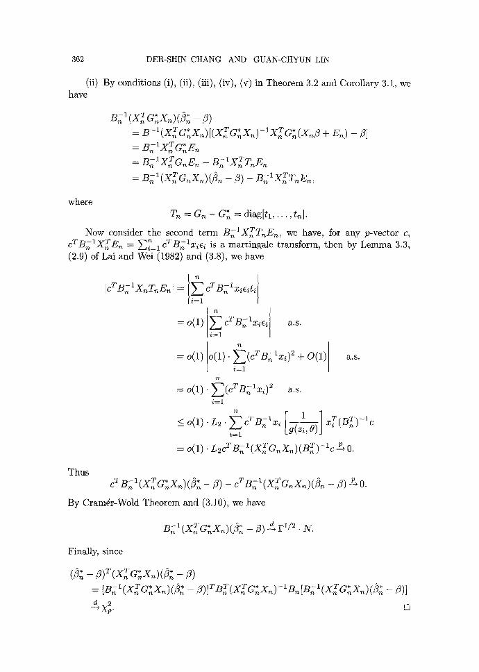
(ii) By conditions (i), (ii), (iii), (iv), (v) in Theorem 3.2 and Corollary 3.1, we have

: B - ~ ( X ~ a ; X ~ ) ~ , -~ ~ , [(X~ a ~ X ~ ) X ~ a~(x,?%9 + E~) - fl] --I T * =B~ X~G~E?%

: BgIxTGnE n - B~IXTTnEn

Bnl(XTn anXn)(~n fl) -i T = - - B n X?% T~En,

where Tn = Gn - G~ = d i a g [ h , . . . , t ~ ] .

Now consider the second term BglX~TnEn, we have, for any p-vector c, cTBglX~E~ = ~-~i~=1 cTB~lxiei is a martingale transform, then by Lemma 3.3, (2.9) of Lai and Wei (1982) and (3.8), we have

[cT Bnl XnT?%En[ = i=< cT Bglx{eiti

n

: o(1) E c T B n l x i e i a.s. i----1

o(1) o ( 1 ) ~ - ~ 2 o ( 1 ) = • (c B ~ x 0 + a.s . i = 1

?%

= O(1) V~(aTB-lx ~2 " ~ \ ~ i] a . s .

i:1

<__o(1).L2.~cTBnlxi [~]xT(BT)-Ic i----I

o(1) T - 1 T T - 1 P = • L~c B?% (X?% a ~ X n ) ( B ~ ) ~--* O.

Thus ~rB-I~xT~*X~ , ~ . ~ ~,~*,~ - 9) - c T B ~ ( X ~ a ~ X ~ ) ( 3 ~ - 9) ~--' O.

By Cram6r-Wold Theorem and (3.10), we have

- 1 T • % _ F ~ / 2 B~ (X?% G~X~)(9~ 9) £ . N.

Finally, since

( ~ ; ~ x ~ * x ~* - fl) ( n c ~ ~)(97% - 9 ) --I T * ^ * T T T * --i --I T * ^ * 9 B X G Xn BnB X G X~ fl- : - )] n ( ~ n ) [ ~ ( ~ n )(7% 9 ) ] [s~ (x~ a~x~)(9;

d 2 --~ Xp. []

STOCHASTIC REGRESSION MODEL 363

4. Hypothesis testing problem

Suppose tha t in model (1.1), E(e2n I -~"n--1) = g(zn,O) where g is a known function of z~ and unknown parameter 0. For the null hypothesis H0 : HT/3 = h against the alternative hypothesis H1 : HT/3 ¢ h where H T is a k x p (k < p) matr ix with rank k and h is a k x 1 known vector, we will discuss this hypothesis as follows.

t E(e2n I hen_l) 1 for Consider the rewrit ten model (3.1), rl~ = w~/3 + en and = every n. Let

]:~g = (@n -- W n ~ n ) T ( ~ ) n -- W h e n ) ,

W , ^ , T = - - w /37 )

where W~ = ( W l , . . . , Wn) T, ~)n = ( 7 7 1 , . . . , ?In) T, )n is the weighted least squares

est imate of/3, and/)* is the constrained weighted least squares est imate of/3 under H0. It can be shown tha t ~ ~- ~,"n{I/VTW'n]~-lW'T~/'n ~ n and ~* = ~ n - ( W ~ T W n ) - I .

H [ H T ( W T W ~ ) - I H ] - I ( H T ~ - h). Let P,~ = W ~ ( W T W n ) - I w T and P* = Wn(wTw~)- IH[HT(WTn W~)-IH]-IHT(WTn W n ) - I w T , then Pn and Pn - P* are the projection operators of M (W~), the space generated by Wn, and the space {W~/3 [ HT/3 = h} respectively. Furthermore, (Pn - P*) is orthogonal to P* (see Chang and Chang (1990)), denote P~o = P~ - P*, then we have

- W , A , T R 1 = ( ¢ n ^* - -

= 11(¢),~ - e w ¢ ~ ) [ I 2 - l i e n - - P , ~ ¢ ~ [ I 2

= I I f , ~ f n - P w C n l l 2

-- ( H T ~ -- h)T[H T (WTWn) -1H] -1 (HT~n -- h)

= (HT~n - HT/3 + HT/3 -- h )T[HT(WTW~)- IH] - I

• (gT~n -- HT/3 + H T z -- h).

Thus under Ho, R~ - R~ = (~n - /3)TH[ HT (WTn W ~ ) - I H ] - I H T (/3n ^ - /3) . Let

(4.1) An = P~W~

then

and

AnT An = H[HT (WTn Wn)- I H]-I H T,

(4.2) R~ R~ ( ~ TAT ^ _ - = - / 3 ) ~A~(/3n /3)

Now we give a test statistic of linear hypothesis H0 : HT/3 = h and construct an asymptot ic distr ibution as follows.

THEOREM 4.1. Suppose that in the regression model (1.1), {%} is a martingale difference sequence with respect to an increasing sequence of or-fields {5~}


such that (2.1) holds and E(e~ I ~ - 1 ) = g(zm 0) where g is a known function of zn and unknown parameter vector 0. Moreover, assume that conditions in Theo- rem 3.2 hold and there exists a sequence of nonrandom nonsingular matrix { Bn} such that

--1 T T --1 Bn (XnGnXn) (Bn) P [ ' ,

where F is a positive definite matrix with

and

T T - 1 P max x i (B~B~) x i ~ O l < i < n

00] (A~A~)(B~) P F 1/2 k F1/2

where Ukxk is an idempotent matrix with rank k. Then under Ho : HT/3 = h, not only R~ 2 - R~ 2 = (~* - / 3 ) T H [ H T ( X T G * X ~ ) - I H ] - I H T ( ~ * --/3) but also R~ - R~

converges in distribution to X 2 as n --+ oo, where ~ and G* as in (3.7), R .2 as

in (4.2) except replacing ~n, 0 by ~* and On, respectively for i = O, 1.

PaOOF. First from (3.9)

~(B B~)-%~ " max w n -+ a.s. l < i < n

then from (4.2) by subst i tut ing/~* for/3~ and A* for An, where A* -- P ' W * as

in (4.1) except subst i tut ing 0~ for 0 in the entries of W~, we have

< 2 _ R;2 ( ~ ,T • ^ , = - / 3 ) ( A ~ A~)(/3 n - / 3 )

~]T[BT{xTG*x ~-1{ B ~] = [~<~(x:atx~)(j~-.,~ ~ ~, ~ n. n, , ~,~

--1 * T * T --1 T T * --1 • (B~ (X~ G~X~) Bn) [Bn (A~ A~)(B~) ]

• [ B n l ( X ~ < X n ) 0 ~ -/3)].

Using Theorem 3.4 and (4.3) we have

a s 7% ---+ (X3.

Secondly, from Lemmas 3.4, 3.6 and 3.7, we have

xTc.x, l=<cnx Tb n 7%}


and

(4.4) *T * (An An) = H [ H T ( X T G * X ~ ) - I H ] - I H T

( 1 ) 1 - 1 : H [ H T ( X T G n X ~ ) - I H + o H T

= n . g [ n . H T ( x T G n X ~ ) - I H + o ( 1 ) ] - l H T

= n . H { [ n . H T ( X T G n X n ) - I H ] -1 + o (1 ) }H T

= H [ H T ( X T G n X n ) - I H ] - I H r + o ( n )

= (ATnA~) + o(n) a.s.

Then from Lemma 3.5, condition (vi), (3.8) and (4.4), we obtain

--1 *T * T T --1 II -<o(n) IIBgl(B~)-III IIB~ [(An A n ) - 1

_< o(n) . A ~ ( n )

i.e.

Bn (An A n ) ( B n )

Using Theorem 3.4 we obtain

- - B-IxTx {B T]-I P O n n n\ n]

0] F1/2'

R 2 R 2 d 2 - ---~ Xk. []

By this result, we can conclude that , in practical, the null hypothesis H0 would 2 for significance level a and in large n. be rejected if R~ 2 - R8 2 > Xk,l-~

5. Example

In this section, we apply our method to the following linear heteroscedastic model. We demonstrate the linear heteroscedastic model of the regression model

T 0, where zn (Znl Z~2, ., Z~k) T is an observable (1.1) with E(e2n I ~c~_1) = z n • = , .. random vector, JCn_l-measurable and 0 = (01, . . . , Ok) T is a parameter vector. In this model, 0n is equal to T -1 T ^2 (Z~ Zn) Z~ e n with Zn = (zij)l<_i<_n,l<_y<_k.

COROLLARY 5.1. Suppose that in linear heteroscedastic model, {c~} is a martingale difference sequence with respect to an increasing sequence of a-fields { ~ } such that (2.1) holds. We assume the conditions (i), (ii) and (v) of Theo-

rein 3.1 are satisfied and liminf~ ~m~n(Z~Z~) > 0 a.s., then On ~ 0 a.s. n

PROOF. check the condition (iv) of Theorem 3.1 whether or not holds.

1 1 lim~__,~ ~ E t = l ( z T ( O - f l ) ) 2 = 0 , from

0 = lim 1 ~ ( T( 1 TZ T _ p ) -- z 0 - - p ) ) 2 = l i m --(O--p) Z~(O n---+oo n n---~o~ n

t = l

_> l iminf •min(ZTZn)II0 - pll -> 0 (by Lemma 3.5) n n

Since the condition (ii) of Theorem 3.1 clearly holds, we only need to Assume


we have 0 = p a.s. Thus, by Theorem 3.1, we have 0n ~ 0 a.s. []

Now we consider a special case of linear heteroscedast ici ty model. Let z~ = (1, u~) T and 0 = (d, or2) T, then g(zn, O) = (72un + d and

(1 Z Zn/n=

n n where ~ = E 1 u~/n, ft 2 = E i u~/n.

Let A = ~ m i n ( Z T Z n / n ) = {i -~- ~2 __ [(1 -- ~2)2 @ ( 2 ~ 2 ) ] 1 / 2 } / 2 , we have

( 1 - g 2 ) 2 + ( 2 g ) 2 = 4 A 2 - 4 ( 1 + g 2 ) A + ( l + ~ 2 ) 2

> - 4 ( 1 + g 2 ) A + ( l + g 2 ) 2.

It implies

A _> [if2 _ (~)2]/[4(1 + g2)]

I > ( n - 1 ) E u / 2 n2 + n u~ .

1

If inf~ u~ = c > 0 then E i = l n ui2 _> nc and

i=1 ?'ti > lim inf - - l iminf ( n - 1)}-~n 2 f t E i = I Ui

nC -- C

n(l + c) > 0

i .e. l i m i n f / ~ m i n ( Z T Z n ) / n > O.

n

Therefore, we reestablish the results of Cheng and Chang (1990) from Corollary 5.1, Theorems 3.2, 3.4 and 4.1.

6 Discussion

Note that in many simulations the convergent rate of t)n converging to 0 in Lemma 3.1 (Jennrich (1969)) are sometime slow, so it is not efficient in application, thus to find a bet ter me thod to subs t i tu te it is necessary in practice. If 0 is permi t ted to contain elements of/3, i.e. 0 = [C~l,..., c~ r ,~ l , . . . , ~p]T, we can find all results still hold under those conditions mentioned before.


Acknowledgements

We would like to thank the referee and associate editor for their many helpful comments and clarifications.

Appendix

In this appendix, we prove Lemmas 3.3, 3.4, 3.5, 3.6 and 3.7.

PROOF OF LEMMA 3.3. Since f is uniformly continuous on compact subsets of A x O, for any P0 E O and any e > 0, there exists 6 > 0 such that f(zt , Po) - e < f(z~,p) < f ( ~ , p o ) + ~ for all ~ e A and l iP- poll~ < 5. Thus, for l iP- poll~ <

sup f(zt , Po) - e < sup f(zt , p) <_ sup f(zt , Po) ÷ e . ztCA ztEA zt@A

Since e is arbitrary SUpz~Zx f(zt , p) is continuous at p = P0, and P0 is arbitrary, so SUpz~E/x f(zt , p) is continuous for all p E O. Similarly, infztezx f(zt , p) is continuous for all p E (9. []

PROOF OF LEMMA 3.4. Since

P

Amax(n)-< E Ai(n) i=1

= trX~Xn = ~ IIx~ll~ = o<~). i=1

[]

Thus

B~CB = (UB)rA(UB)

= ( U B ) T [ A - An(C) × Inxn](UB) @ (uB)T[An(C) × Inxn](UB).

Further since (UB) r [A-An (C) x Gxn] (UB) is nonnegative definite and by Weyl's inequalities, for i = 1, 2 , . . . ,p, we have

A{(B~CB) >_ Ad(UB)r[An(C) × I.×n](UB)} = A{(An(C). B~B)

On the other hand,

(UB)T[AI(C) × Inxn](UB) = (UB)TbI(C) × ±~×n - a](UB) + (UmTa(Um.

Ai(BTCB) < Ai(AI(C)BT B). []

PROOF OF LEMMA 3.6. From, l[A~ 1-B<ll[ < ]IB~iillIAn-Bn]IIIA~1[l and l iminfn Amin(An) > 0, we have A< ~ = Bn I if- o(1) a.s. []

PROOF OF LEMMA 3.5. Since C is symmetric, there exists orthogonal matrix u such that C = UTAU where A = diag(Al(C), A2(C) , . . . , An(C)), we have


PaOOF OF LEMMA 3.7. Let ~,~ = {w : sup~llxn(w)llp < m}, p (U,~=I ~m) = 1, and let

1 1 g(zt , O) - 9(zt , p) h(z , , p) - g ( z , , , ) g ( ~ , O) - g(~,, O)g(~ - p)

1 < 1 < 1 { 0 , 0 1 , . . 0n, .}. Thus we have by assumption ~ _ ~ _ z-[Vp E ., ..

l ~ {g(zt'O)-g(zt'P)) 2 1 h2(zt'P) • n \ -~t,O-)g(g --- fi) n t : l t : l

n

1 1 t~l(9(zt, O) - 9(zt, p))2Vp E {0, 0 1 , . . } <- L ~ ~

from the proof of Theorem 3.1, we have

and

n

1 E(g(zt,O) g(zt,O~)) 2 o(1) ?%

t = l

1 ~h2(zt,O~) o(1) n

t = l

a.s.

a .s .

Now

l X f<E~ IxfG.E~ - n n

!X~(Vn-- G~)E~ n

1 ~ h(zt, On)et - - X t l •

n t = l

n

1 F_, x~ h(z~,<)~ n

t = l

n

1 E xtp h(zt, On)ct n

t = l p x l

for k = 1 , 2 , . . . , p , and

1 E x2tkh2(zt'On) <- ml-n h2(zt'On) = 0(1) t = l t = l

a . s .

By Lai and Wei (1982) (2.9), we have

l Zx~kh(z~,<)~ --o Gh2(z~,< + O(1) o(1) n t = l n t = l

a . s .

then


and

Hence

Next

1 T • -X~ G~E~ = IXTG~E~ + o(1) n n

1 T • - X n G,~E~ = 1XTGnEn + o(1) n n

a.s .

a . s .

1 ± T • m anXn ZxfGnx n n

n I Xtlh(Zt , On)Xtp _1 E xtlh(zt, On)xtl,. " " ' -n r~ t = l =

n

1 E x t p h ( z t , O n ) X t l , . 1 E x t p h ( z t , On)Xt p ) n t = l ft t = l

for 1 _< h, k _< p, and by Cauchy-Schwarz inequality

t=l

<-m21 -nl ~h2(z t , = o(1) a.s.~

we have 1 T * -- 1 x f + o(1) n n

Hence 1XTG*X~= !XTG~Xn +o(1) ?~ n

Finally, from Lemmas 3.5 and 3.6, we have

a .s .

a . s .

1 - 1 - 1

a.s . []

R E F E R E N C E S

Chang, D. S. and Chang, M. R. (1990). Hypothesis tes t ing in s tochast ic regression models, Tech. Report , Nat ional Tsing Hua University.

Cheng, M. I. and Chang, D. S. (1990). A note on s tochast ic regression model wi th heteroscedast ic d is turbances , Tech. Report , Nat iona l Tsing Hua University.

Jennrich, R. I. (1969). Asympto t i c proper t ies of non-l inear least squares es t imators , Ann. Math. Statist, 40, 633 643.

Lai, T. L. and Wei, C. Z. (1982). Least squares es t imates in s tochast ic regression models wi th appl icat ions to identif icat ion and control of dynamic systems, Ann. Statist., 10, 15~166 .

Documents

Ann. Inst. Statist. Math. - 統計数理研究所 · ann. inst. statist. math. vol. 47, no. 2, 351 369 (1995) stochastic regression model with heteroscedastic disturbance* der-shin