ANNEX B: ELEMENTS OF RELIABILITY THEORY AND APPLICATIONS TO SAFETY ANALYSIS

B.1 INTRODUCTION

The aim of this chapter is to provide the main tools for understandingthe application of the techniques of reliability on safety studies.Therefore, after recalling the definition of the main variables usedin the reliability analysis, the focus will be on assessing thereliability of components and systems, simple or complex. Itwill also briefly examined a crucial aspect for applications: thecommon causes of failure and human error.Obviously we are not going to do a full discussion of the reliabilitytheory and application techniques to the analysis of complex systems,but only introduce this theme, with sufficient understanding of its usein the safety analysis. For further information and more details, seethe books mentioned in the references.

B.2 DEFINITIONS

Failure rate (t): fraction of components that fail per unit of time;Reliability R (t): probability that an apparatus performs the taskassigned in a specific time interval (0-t), under certain environmentalconditions;Unreliability Q (t): probability that the equipment has failed duringthe considered time interval (0-t) (it does not carry out the functionassigned at the instant t, for a fault occurred at any instant in theinterval 0 -t);Availability A (): probability that the system is operating properlyduring the mission time Unavailability I (): probability that the system is not able to performits function during the mission time , namely fraction of for which,an average, the system is defective (Relative Dead Time).

B.3 CLASSIFICATION OF COMPONENTS FAILURES To determine the reliability of components produced industrially inlarge quantities (eg. electrical components, such as resistors,

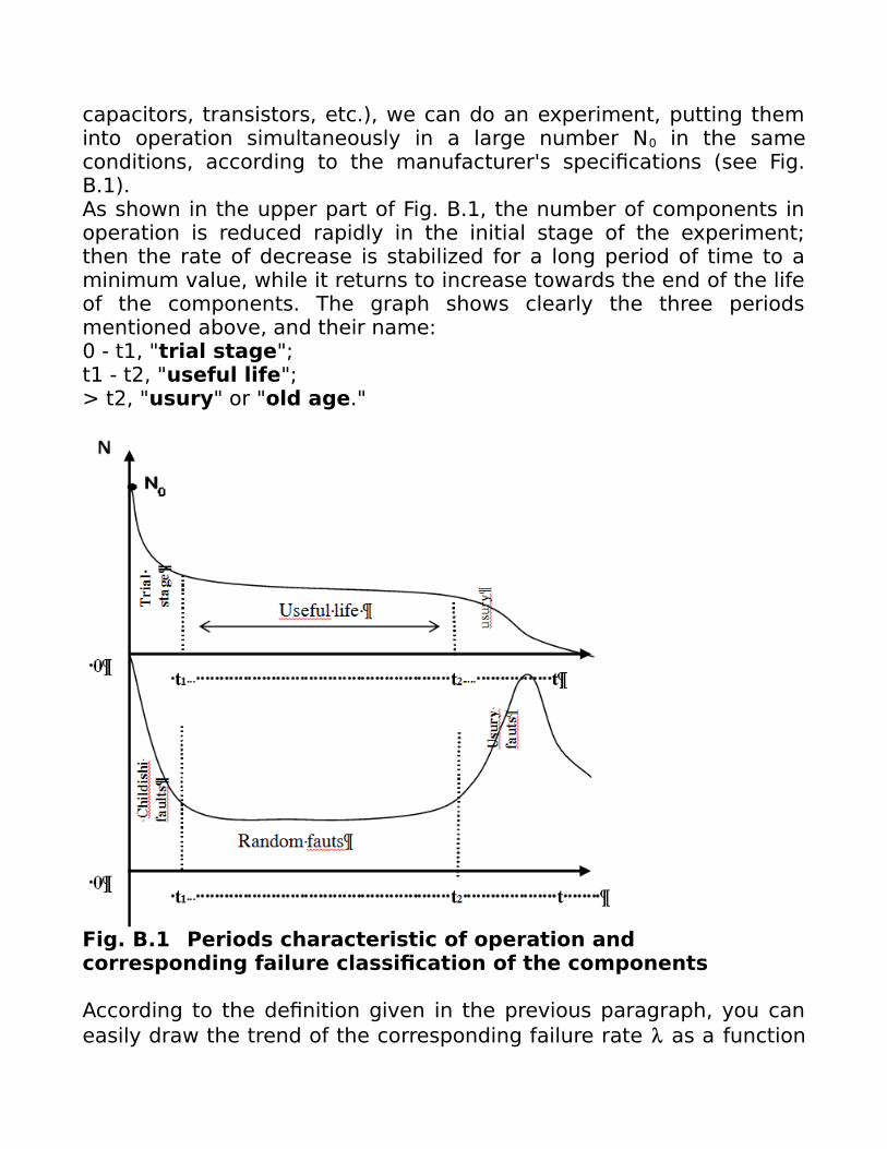
capacitors, transistors, etc.), we can do an experiment, putting theminto operation simultaneously in a large number N0 in the sameconditions, according to the manufacturer's specifications (see Fig.B.1).As shown in the upper part of Fig. B.1, the number of components inoperation is reduced rapidly in the initial stage of the experiment;then the rate of decrease is stabilized for a long period of time to aminimum value, while it returns to increase towards the end of the lifeof the components. The graph shows clearly the three periodsmentioned above, and their name:0 - t1, "trial stage";t1 - t2, "useful life";> t2, "usury" or "old age."

Fig. B.1 Periods characteristic of operation and corresponding failure classification of the components

According to the definition given in the previous paragraph, you caneasily draw the trend of the corresponding failure rate as a function

of time, shown in the lower part of the same Fig. B.1, It is the well-known curve "bathtub", leading to the classification componentfailures in:"childish", due to defects and imperfections of construction that areevident readily during the break-in period, leading to the exclusionfrom the use of components that are affected;"random", during the period of useful life, corresponding to a rate offault minimum and almost constant;"usury", during the corresponding period and due to the deteriorationof the characteristics of the component by the stresses to which hasbeen subjected during operation.

Previous observations imply that for optimum reliability, it isnecessary to make a proper break-in components, using the sameonly during the period of useful life; consequently it is also necessaryto perform maintenance operations programmed, by replacing thecomponents which have reached the end of their useful life. Only bydoing so you can rely on a minimum and also almost constant, intime, failure rate for the components used.

B.4 ASSESSMENT OF COMPONENTS RELIABILITY

B.4.1 Non repairable components

Assuming, as usual engineering practice, that is possible toapproximate the probability with the observed frequency (hypothesisacceptable if the statistical basis is sufficiently wide), the reliability isgiven by the relation:

R (t) = N / N0 (B.1)

where N is the number of components "survivors" at time t, and N0 isthe initial number of components at the time t=0.

Similarly, the unreliability is expressed by the relation:

Q (t) = 1-R (t) = Ng / N0 (B.2)

where Ng is the number of failed components between the initialinstant and the generic time t.

Note that the two relationships listed above are valid for non-repairable components, or that, once they faults, remain in a state offailure for the whole duration of the observation.The definition of the failure rate can be expressed with therelationship:

(B.3)

from which, according to (1) is immediately obtained:

(B.3’)Solving:

(B.4)and under the assumption that is constant over time:

R = e -t ~ 1-t if t<<1 (B.4’)

According to the fundamental theorem of probability theory wetherefore have:

Q (t) = 1 - e -t ~ t if t << 1 (B.5)

In the study of a system composed of non-repairable components (eg.missile, etc.), the probability that the system fails during the missiontime will be given by Q(). Furthermore:

A() = R() and I() = Q() (B.6)

The assumption of constant (and minimum) failure rate is generallyvalid for units (1) that have been passed the break-in period(elimination of defects "childish", namely due to defects in theconstruction, trivial errors, etc.) and are used during the period of"useful life", before they will overtake the usury. Using always processunits in the period of useful life (and then by making systematic andscheduled maintenance, with units replacement at the end of theiruseful life), the mean time between failure period (MTBF - MeanTime Between Failures) is: MTBF = 1/ (B.7)

More generally one can demonstrate the validity of the followingrelationship:

(B.8)

valid whatever the mathematical expression of R (t).The previous definitions and relationships extends easily to the caseof process units with cyclic operation, with the replacement of theMTBF with the average number of cycles of correct operation "c" (tobe put in previous relationship (B.7) in place of 1 / ).

B.4.2 Repairable components

Differently from the previous case (and most interest cases for theindustry), the failing component is usually repaired (or replaced) andput back into operation. In this case, it becomes important theconcept of Mean Time To Repair (MTTR), namely the time intervalduring which the component remains in a fault state.Similarly to the failure rate, it can be defined a repair rate m:

m = 1/MTTR (B.9)

For repairable components the availability is therefore defined as:

1 In this chapter, the term "unit" is meant indifferently component, equipment or system.

A = MTBF / (MTBF + MTTR) (B.10)

and analogously the unavailability as:

I = 1 - A = MTTR / (MTBF + MTTR) = (B.11)

B5 RELIABILITY OF PROTECTION AND SAFETY SYSTEMS

For equipment and systems devoted to protection and safety, it isnecessary to premise a further classification of types of failure:• faults in favor of safety (fail safe), namely involving theintervention of the unit in the absence of a dangerous situation. Inconsequence of an intervention "fail safe", the plant changes statefrom that of normal operation to a situation of greater safety. Thisautomatically reveals the failure of the unit.• faults to the detriment of safety (fail to danger), which involvethe non-availability of a unit in the event that it be called to operateas a result of a failure (demand) of the process system.

The faults fail to danger can be revealed (and in such case promptlyrepaired) or not revealed; in the latter case they can be detectedonly by a request of the process system (which cannot be satisfiedand therefore result in an incident) or from an ad hoc test at the endof the mission time. Clearly, as the risk of incidents arises mainly fromoccurrence of faults fail to danger, the designer puts a certain cure inminimizing the relative failure rate, particularly for faults not revealed.

We have already mentioned that an incident in a highly dangerousplant occurs only for the concomitant occurrence of a fault in thesystem process (demand) and the failure of the system for protectionand safety. Hence the definition of "unavailability" of a safety andprotection system such as probability of non-interventionfollowing a request of the process system. In this way theprobability of occurrence of an accident is given by the product of theprobability of failure of the process system for the unavailability of theprotection system.

For protection system failures "fail to danger" unrevealed, it is easilyto demonstrate that the unavailability for a mission time (intervalbetween two successive tests, which can reveal the faulted protectionsystem) is given by:

(B.12)Ultimately this relation expresses the fact that I is the average valueof Q (t) within the mission time. I is also equal to the Relative DeadTime, namely the fraction of the time for which on average theprotection system is broken:

(B.13)

In the previous relation dQ is the probability that the protectionsystem fails at a generic instant t, in which case remains faulted forthe remaining interval (t-).In the case of a protection system with exponential reliability:

Q (t) = 1 - e-t ~ t if t << 1and:

~ (B.14)

In the previous expression it is implicitly admitted that the tests are allperfect and of infinitesimal duration (namely negligible compared to). With this hypothesis would be sufficient to reduce the time intervalbetween two tests to reduce accordingly, as you want, theunavailability of the protection system, in accordance with (B.14). Atthe limit, by tending to zero, I also tends to zero, against the obviousconclusion that if a system of protection is constantly under test, it isnever available to perform its function (and therefore hasunavailability equal to 1).Introducing the test duration t (and including in t the repair timewhen the test reveals a fault), the previous relationship becomes:

(B.15)

given the fact that during the test the system is not available and itsQ is 1. The latter relationship is suitable to an optimization of theinterval between two successive tests; The minimum is obtainedderiving equation (B.15) and putting the derivative to 0:

(B.16)from which:

(B.17)By substituting this optimum mission interval in (B.15), we have:

(B.18)

Previous conclusion is consequence of the hypothesis of perfecttesting (which do not introduce faults). This hypothesis can beremoved, assuming that is function of the number of tests andincreases by increasing the number of tests:

= 0 . f () (B.19)

The simplest expression for (B.19) is

= 0. (B.19')

that, by substituting in (B.16), leads to the relationship:

(B.20)

To conclude this section we have to treat the case of a systemmalfunction fail to danger revealed. The solution of the problem isimmediate, remembering that unavailability is equal to the RelativeDead Time and therefore the relationship (B.11) holds, already seen inthe case of repairable parts. In addition it is implicit the assumptionthat the plant continues to be operated during the repair time. In thecase of installations with a high hazard, this can be admitted only if

there are other safety systems capable of carrying out the functionperformed by the system under repair.

B.6 RELIABILITY ASSESSMENT OF 'SIMPLE SYSTEMS

The most common cases of reliability and unavailability calculation, inthe field of safety reporting, are those schematized with the seriesand parallel logics. Any case also other logics are used, as themajority and reserve ones.

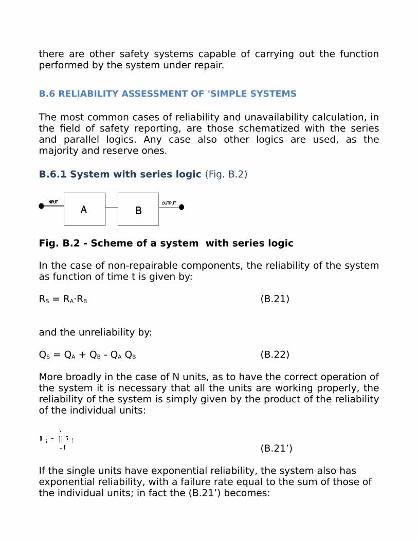
B.6.1 System with series logic (Fig. B.2)

Fig. B.2 - Scheme of a system with series logic

In the case of non-repairable components, the reliability of the systemas function of time t is given by:

RS = RA·RB (B.21)

and the unreliability by:

QS = QA + QB - QA QB (B.22)

More broadly in the case of N units, as to have the correct operation ofthe system it is necessary that all the units are working properly, thereliability of the system is simply given by the product of the reliabilityof the individual units:

(B.21’)

If the single units have exponential reliability, the system also has exponential reliability, with a failure rate equal to the sum of those of the individual units; in fact the (B.21’) becomes:

(B.21’’)

where:

(B.23)

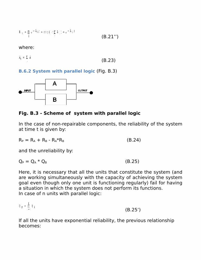
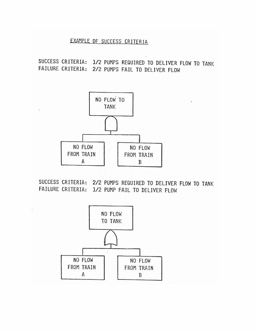
B.6.2 System with parallel logic (Fig. B.3)

Fig. B.3 - Scheme of system with parallel logic

In the case of non-repairable components, the reliability of the systemat time t is given by:

RP = RA + RB - RA*RB (B.24)

and the unreliability by:

QP = QA * QB (B.25)

Here, it is necessary that all the units that constitute the system (andare working simultaneously with the capacity of achieving the systemgoal even though only one unit is functioning regularly) fail for havinga situation in which the system does not perform its functions.In case of n units with parallel logic:

(B.25’)

If all the units have exponential reliability, the previous relationship becomes:

(B.25’’)

(B.24’)

In the particular case, of practical interest, of n equal units thatconstitute the system,with t << 1, the relationship (B.25") becomes:

Qp = (t) n (B.25''')

Even if the components A and B have constant failure rate, theparallel system is characterized by a failure rate function of the time:null at the initial time, then increases, more or less rapidly, to thevalue corresponding at the component more reliable (with lower ).

B.6.3 Systems with majority logic

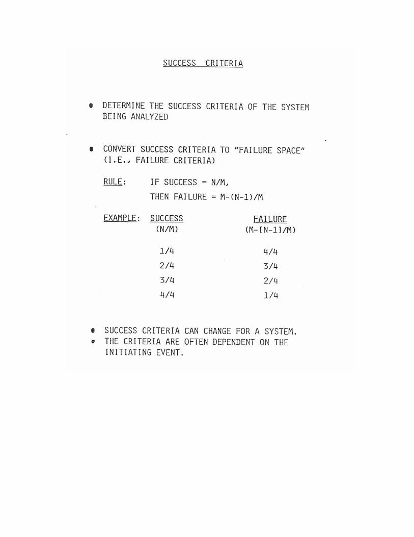
A third case of elementary logic, of considerable practical interest forthe realization of safety systems, is that of the majority logic. Suchlogic allows to keep the advantages of the parallel logic minimizingthe number of spurious trips of the system for faults "fail safe".The reliability of a system with majority logic m/n (i. e. in which for thefunctioning of the system it is required the correct operation of munits on n available) is immediately obtained from the development ofNewton's binomial formula:

(R + Q) n=1(B.26)

If R and Q are the reliability and unreliability of the single unit, in thelast expression the first term is the probability that all units areworking properly, the second is that (n-1) units are working properlyand any one fails , etc. . Therefore, the reliability of the system withlogic m/n is given by the sum of the first (m + 1) terms of (B.26), whilethe unreliability is the sum of the remaining (n-m) terms:

(B.27)

If we denote by r = n-m + 1 the minimum number of units that must fail because the system fails we obtain:

(B.28)

In the usual case of units with exponential reliability, with t << 1, equation (B.28) can be approximated by the first term:

(B.28’)

A particularly important case is the logic 2/3; in this case the (B.28') becomes:

(B.29)

B.7 THE UNAVAILABILITY OF REDUNDANT SAFETY SYSTEMS

For systems with series logic, the treatment done in the precedingparagraph B5 (relationships from (B.12) to (B.20)) for the case of anindividual apparatus are immediately applicable.The unavailability for faults fail to danger unrevealed of systems withparallel or majority logic is obtainable by applying the generalrelationship (B.12); for example, in the case of the logic 1/2 andparallel (with the usual approximations, valid for t << 1), we have:

(B.30)

Similarly in the case 1/3, one can achieve immediately the following result:

(B.31)Taking into account the contribution of testing and maintenance, inthe case of test and maintenance (of average duration t) carried outsimultaneously at the end of the mission time the relationship (B.30)becomes (2):

(B.32)

This case is really theoretical and substantially irrational; if you havetwo units, in order to have always at least one unit running, you canstagger the tests of the two units. The smallest unavailability isachieved by stagger tests of /2; then (Fig. B.4), the unreliability ofthe first unit is given by the usual Q '= t, while that of the second(after commissioning the test at the instant - / 2) is Q " = (t + / 2),from which:

Qp = 2t(t+/2) (B.33)

in the interval where both units work, and

Qp = t when a unit is under test.

The evaluation of the unavailability can be made with reference to theinterval 0-/2, being the situation clearly repetitive (Fig. B.4):

(B.34)

By developing the (B.32) and unless than infinitesimals of higher order, we obtain:

2 In this and in subsequent pages the apex "pc" stands for "contemporaneous tests", the apex "ps" for staggered tests.

(B.35)

By comparing this relationship with the (B.32), one can immediatelysee that the term due to the faults fail to danger not detected of thetwo units is reduced by a factor of 8/5, while the contribution of thetests and maintenance is reduced by some orders of magnitude.By operating in a similar way in the case of logic 1/3, it is easily shownthat, in case of tests and maintenance contemporary in the 3 units,the unavailability is given by the relation:

(B.36)

while with tests staggered at intervals equal to / 3, one achieves the following result:

(B.37)

smaller than the previous one by a factor 3 for the part due to failuresof the various units and several orders of magnitude with regard tothe contribution of the tests and maintenances.

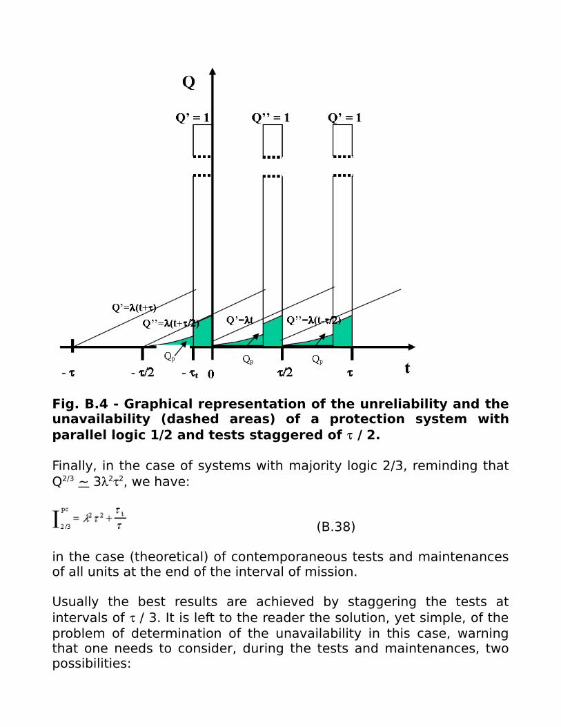
Fig. B.4 - Graphical representation of the unreliability and theunavailability (dashed areas) of a protection system withparallel logic 1/2 and tests staggered of / 2.

Finally, in the case of systems with majority logic 2/3, reminding thatQ2/3 ~ 322, we have:

(B.38)

in the case (theoretical) of contemporaneous tests and maintenancesof all units at the end of the interval of mission.

Usually the best results are achieved by staggering the tests atintervals of / 3. It is left to the reader the solution, yet simple, of theproblem of determination of the unavailability in this case, warningthat one needs to consider, during the tests and maintenances, twopossibilities:

- the unit under test is excluded and the logic becomes 2/2; in thiscase the system has unreliability sum of those of the remainingunits: Q = t + (t + /3) = 2t + /3;

- the unit under test is replaced by a signal in the shutter releaseposition, for which the logic of the remaining units becomes 1/2: Q= 2t (t+/3).

A remark deserves explicit considerations, about the fact thatrelationships (B.35) and (B.37), valid for tests staggered, seem not toallow optimization of the mission interval (on the contrary, this ispossible in the case of contemporaneous tests and repairs -relationships (B.32), (B.36) and (B.38)). In this regard it can be statedthat:

• staggering the tests, the optimization problem for is less importantbecause, during the test drive, one (or more) unit remains operational;• optimization is still possible, but in the development of relationships(B.35), (B.37) or similar one must include the infinitesimal terms forhigher order omitted in previous formulas.

To complete this section, it should be noted that the all the previousformulas (and the similar one valid in case of logics 1/4, 2/4, etc.)assume the complete independence between the various units, neverfully achievable. Usually, there are dependencies between the variousunits due to design, construction and installation, to the location onthe system, etc. These dependencies will ultimately result in a finiteprobability of common failures or otherwise contemporary loss offunction; this probability is orders of magnitude greater than thatcalculated in the hypothesis of complete independence of the variousunits. Operational guidance on this topic (which is critical for riskanalysis) is a very important topic.

B.8 METHODS FOR THE RELIABILITY ANALYSIS OF COMPLEX SYSTEMS

In order to study the probability of failure of a complex system severalmethods have been developed. These, in addition to being a(relatively) simple calculation tool for obtaining this probability, alwaysprovide qualitative information also of considerable importance for

the knowledge of the system and allow then to make decisions basedon a knowledge, as far as possible complete and correct, on thesystem under examination.The main techniques used for this purpose, on which we will focusbriefly at application level, have already been introduced in previouschapters: the fault tree and events tree, logic diagrams borrowedfrom the decision theory.

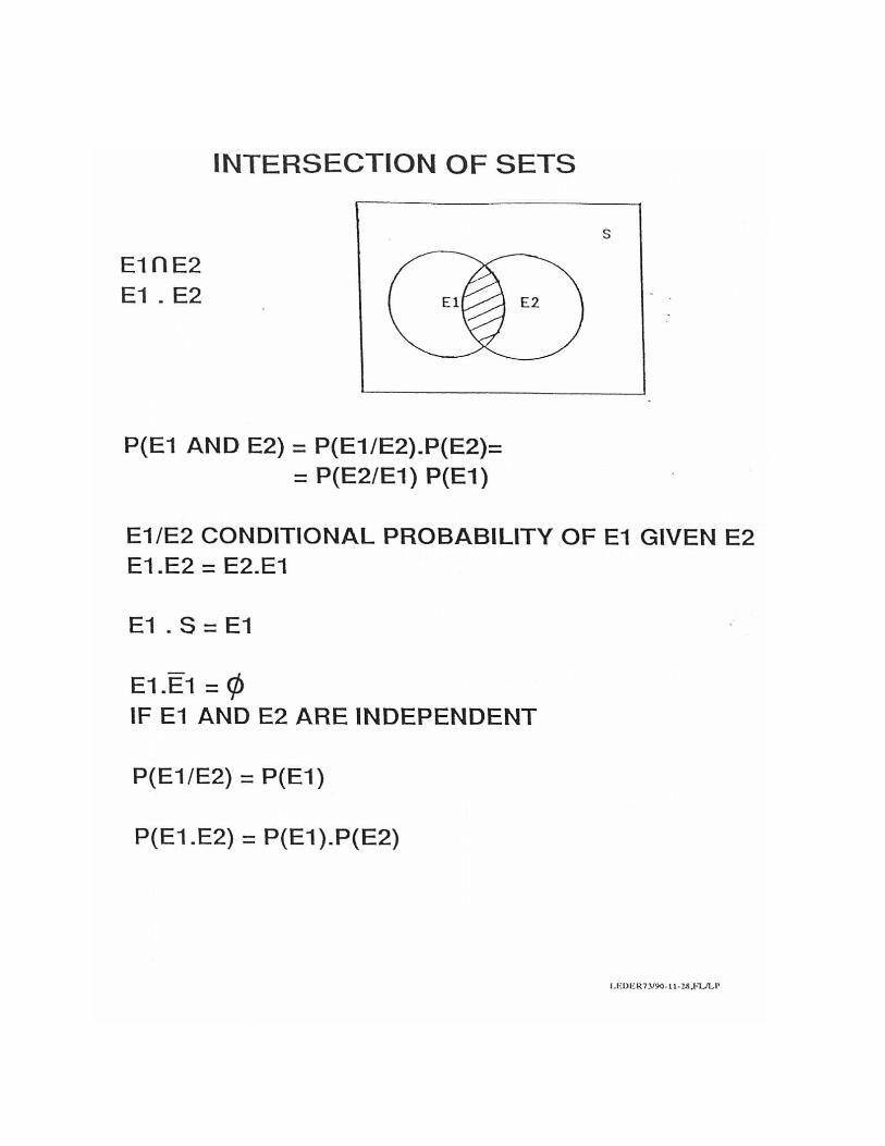
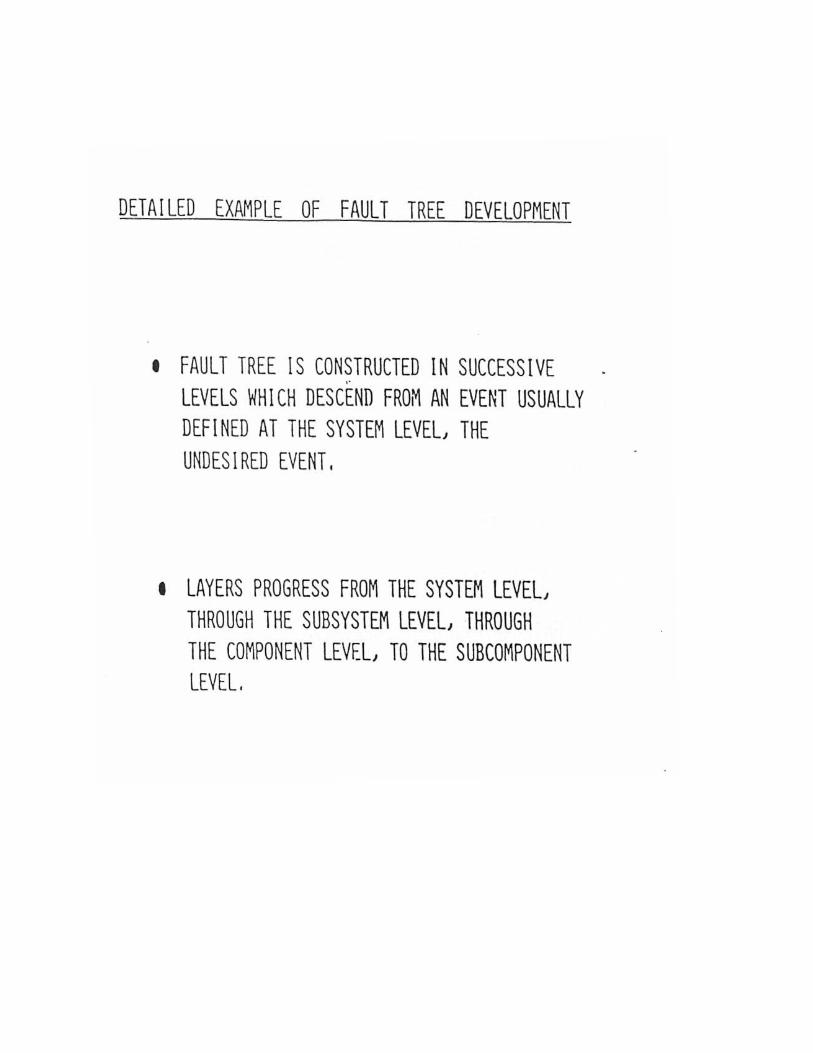
B.8.1 Fault tree method

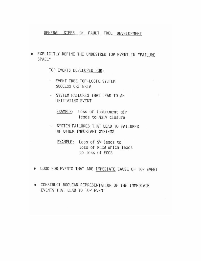
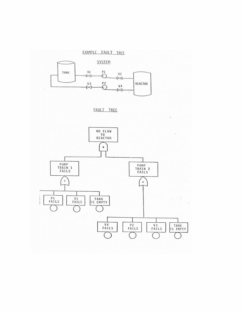
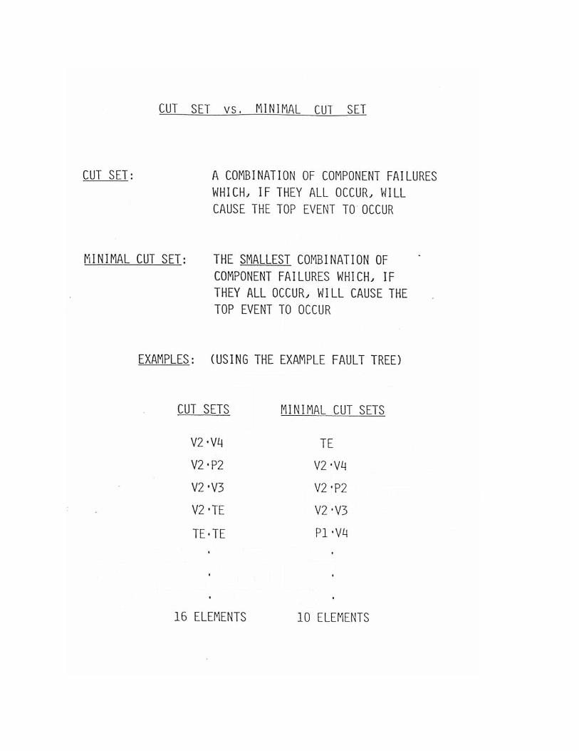
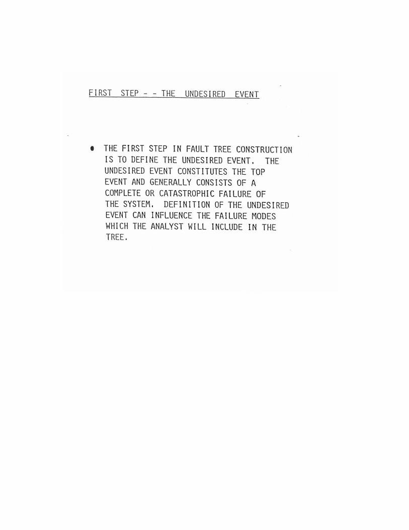
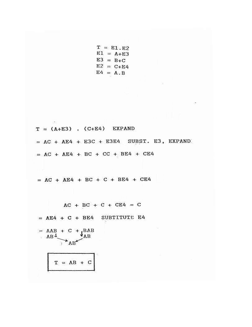
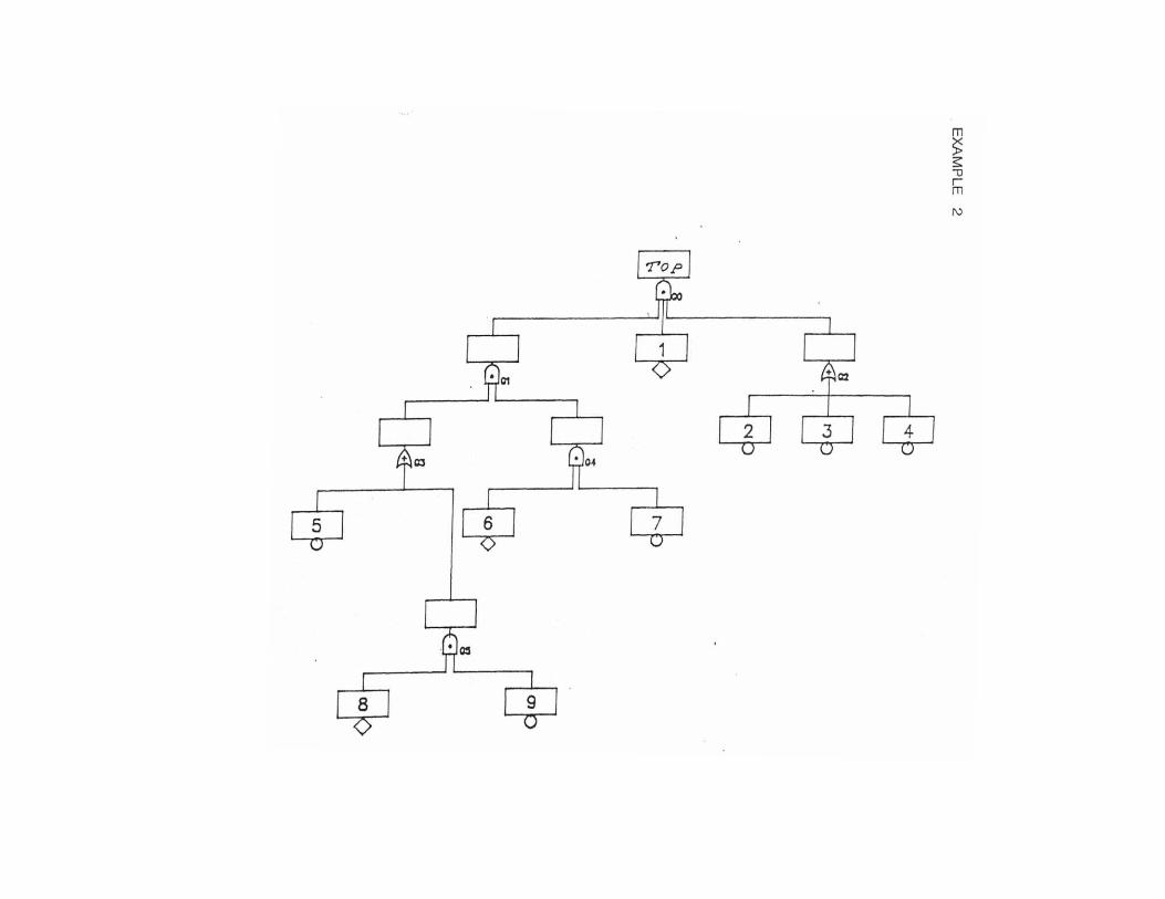
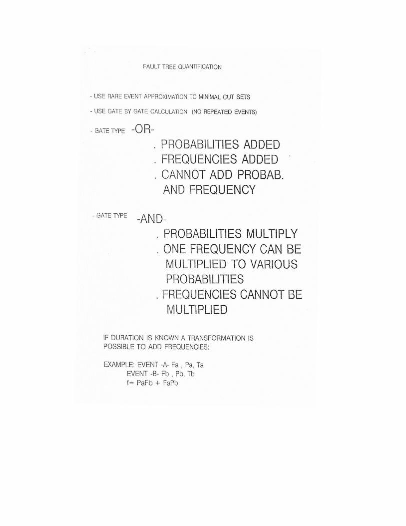
The fault tree is a deductive technique that analyzes a particularevent ("Top Event") for identify the causes.For a proper construction of the fault tree of a complex system it isappropriate the use techniques such as the Hazard and OperabilityAnalysis (HAZOP) and FMEA (Failure Mode and Effects Analysis), thathelp identify the "Top Events" and the logical structure thatdetermines them through a comprehensive and consistent analysis ofthe system.The analysis by fault tree proceeds through the following steps:- Construction of the tree;- Qualitative analysis: solution of the logic tree by applying therules of Boolean algebra, for the identification of "minimal cuttingsets " ("Minimal Cut Sets-MCS") of the system;- Quantitative analysis: solution of the unavailability of the "TopEvent" or of the expected number of events during the mission time,as the sum of the unavailability or of the number of events of theindividual "MCS".

A minimum set of cutting (MCS) is a combination of events, not furthersubdivided (hence the adjective "minimum"), whose occurrenceinvolves the occurrence of the "Top-Event". The fault tree analysisallows the detection of events that can lead directly to the "Top Event"(MCS of the first order), the MCS of order 2 (for which is required theoccurrence of two independent events), etc .; at the end you can alsolist the different "Minimal Cut Sets" in order of relative importance(contribution to the probability of occurrence of the "Top Event").

The rules of Boolean algebra are recalled in Appendix B.1, while anexample of application of the fault tree method is shown in AppendixB.2.

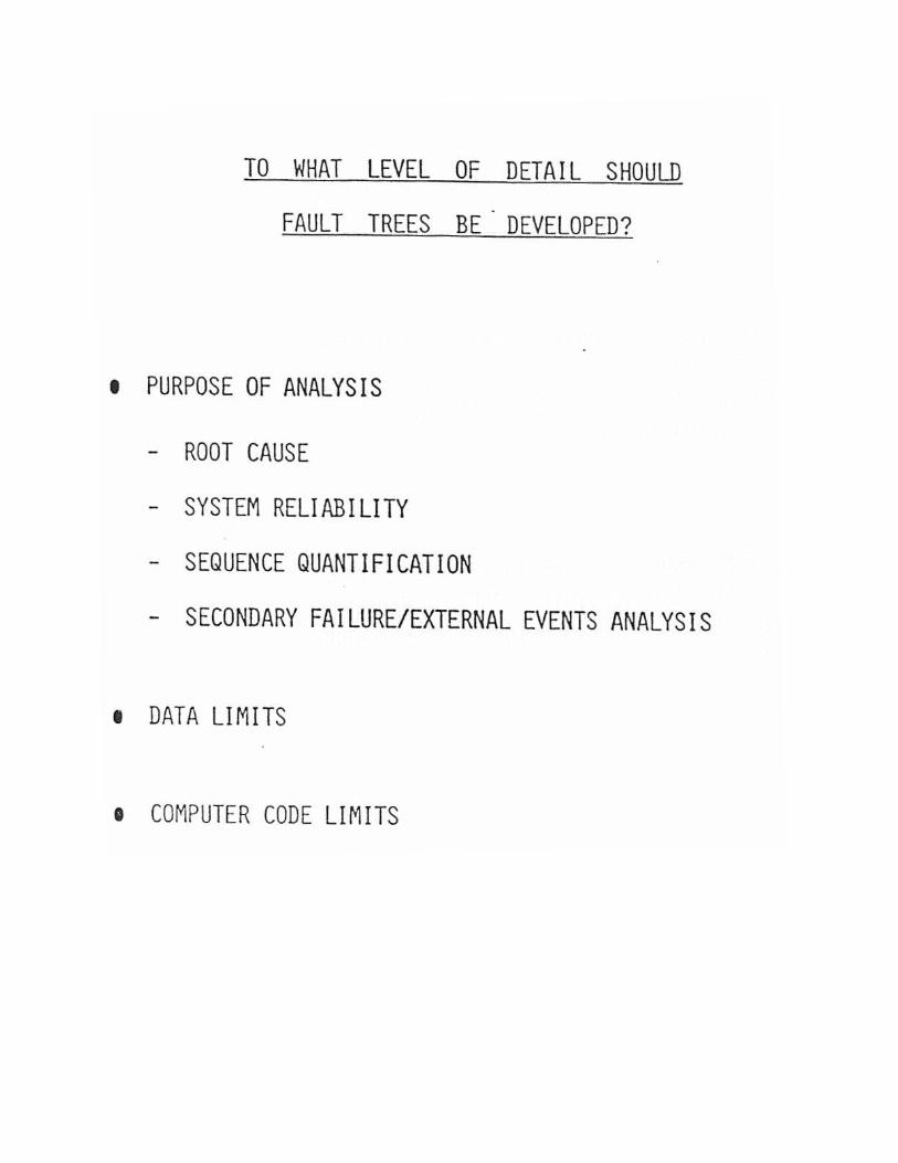
The fault tree is currently perhaps the most used tool in the field ofsafety analyzes for the study of the causes of accidents, theidentification of the most critical components for the assessment ofthe effects of different maintenance policies (time intervals betweentests, etc.) and to quantify the probability of an accident.

Note: the fault tree technique assumes that all basic events listed areindependent. In reality this is not always true (e.g. componentswhere the probability of failure depends on the state of failure orperformance of another component, or dependencies caused bymaintenance). These causes of dependence must be taken intoaccount with the adoption of appropriate techniques.

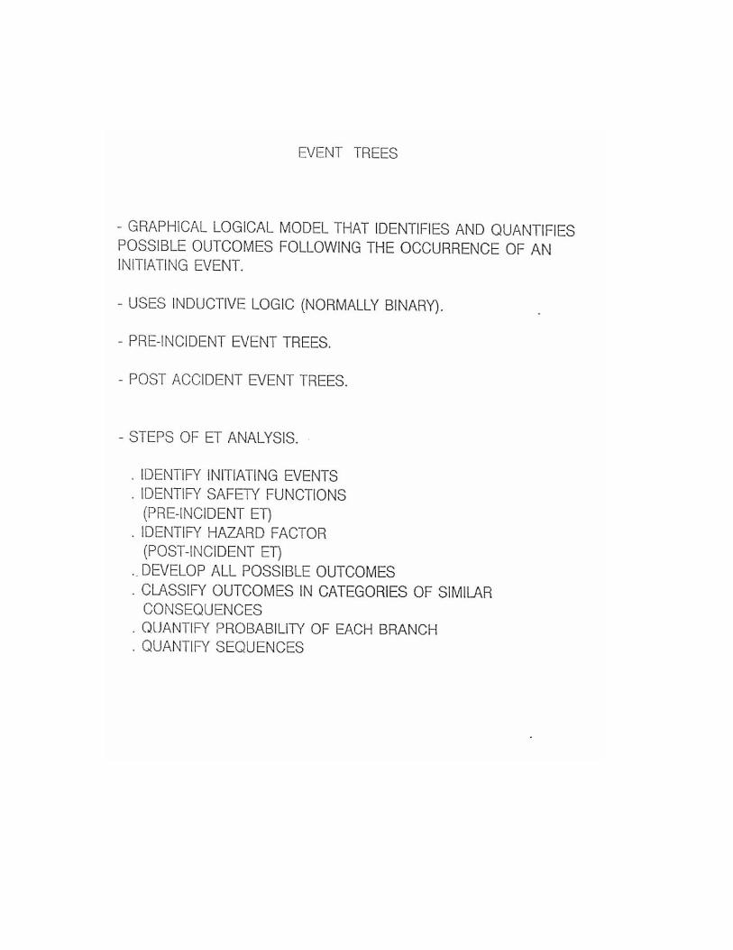
B.8.2 Event Tree Method

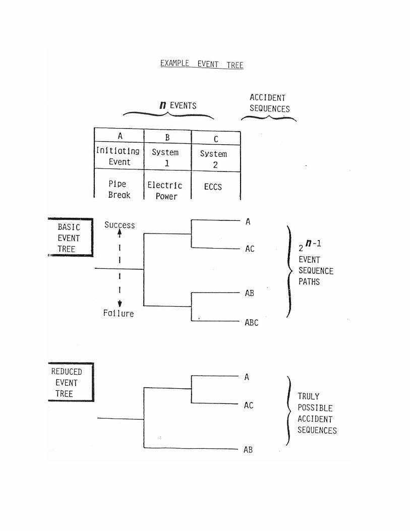
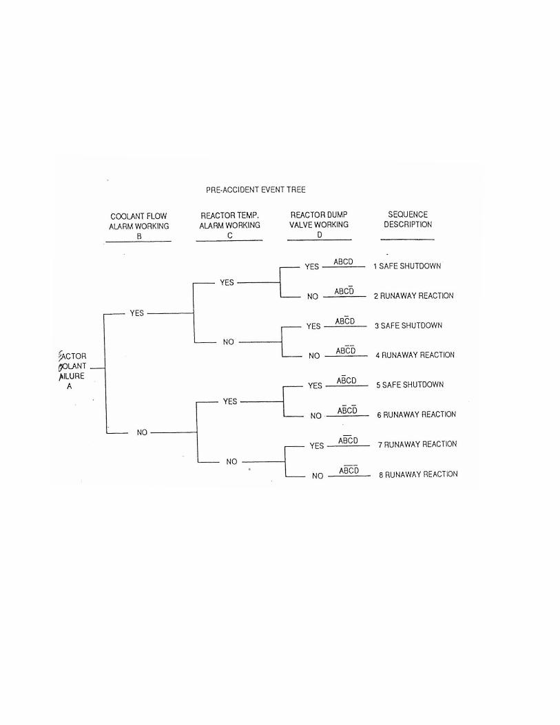
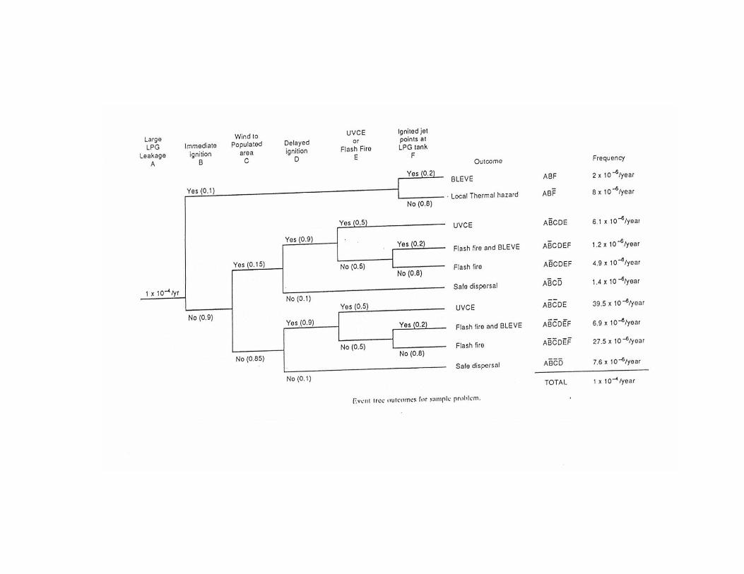
In contrast to fault tree, the event tree technique is an inductivemethod which, from the knowledge of the possible states ofcomponents, enables to build the set of all possible "stories" of thesystem.The logical process start on the assumption that a certain event(initiating event) has occurred; then the tree is constructed studyingall the possible ramifications, depending on the success or not ofaction of various protection systems.

The stories constructed by the event tree are mutually exclusive andare caused by the simultaneous occurrence of all events belonging tothe branch of the tree that defines them. Their probability is thenexpressed as a product of the probabilities of the nodes of the tree;the probability of more stories is the sum of the probability ofoccurrence of each individual story.

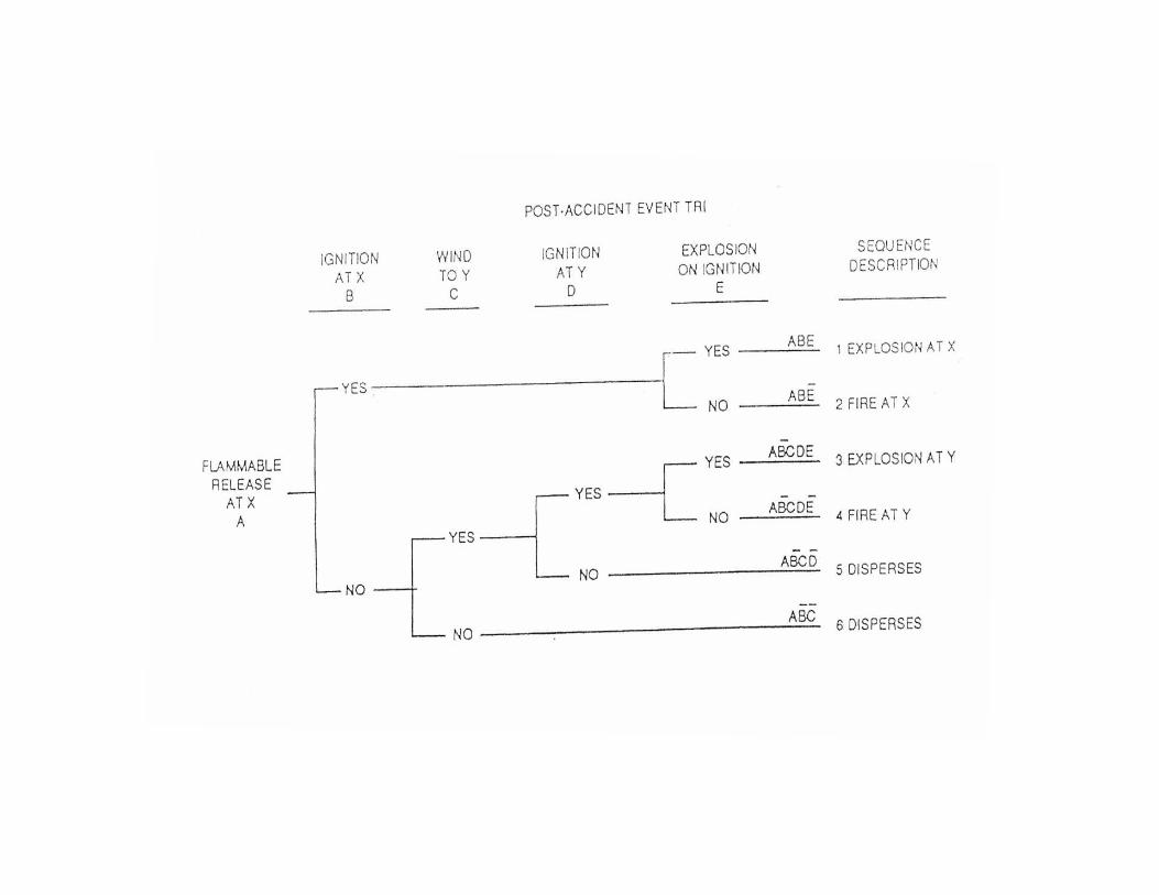
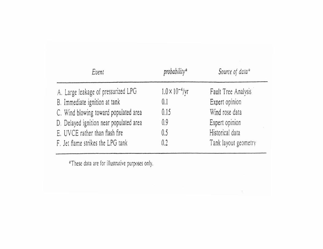
Differently from the fault tree, the event tree method allows to treat,with greater flexibility, dependencies between events and to simulatethe variation of the probability of an event as a function of theoccurrence or not of previous events. In this regard, see theexplanatory example shown in Appendix B.3.Within the framework of safety analysis, currently the event treefounds aso application in the analysis of phenomenologies consequent

to an event (e. g., study of the probability of the different possiblescenarios resulting from a given release, in dependence of thepresence of ignition, of particular weather conditions, etc.).

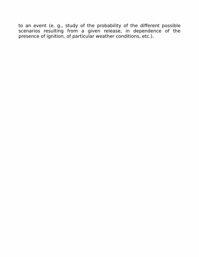
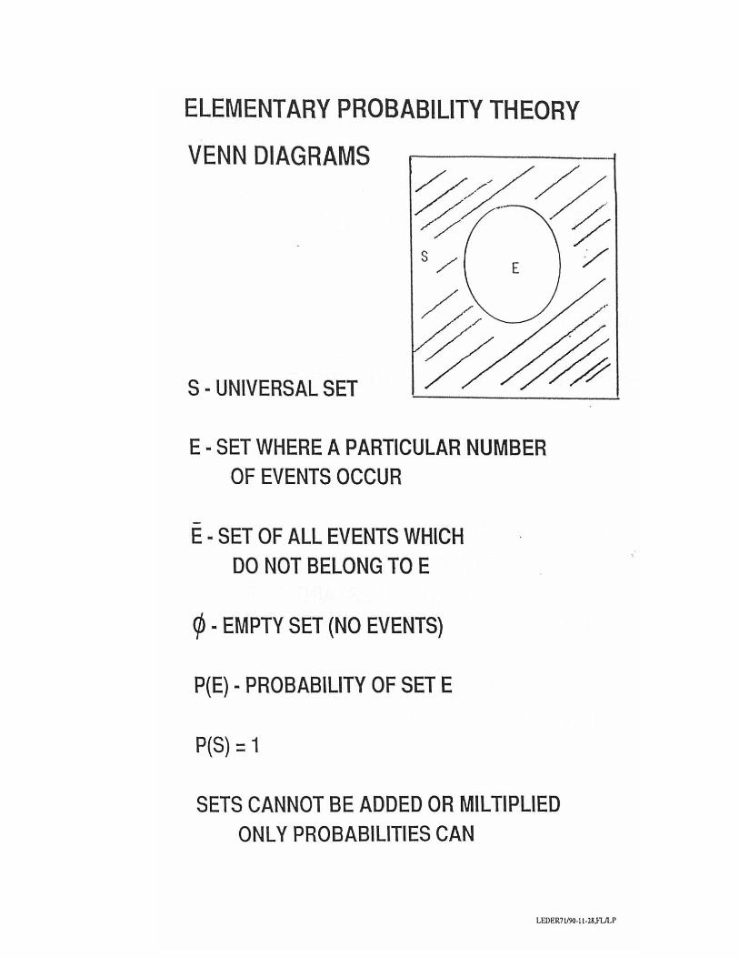
Appendix B.1 Elements of Boolean Algebra

Appendix B.2 Fault Tree Development and Application

Appendix B.3 Event Tree Development and Application